2.1. Notation

Let $ (\mathsf{X},\mathcal{X})$ be a measurable space. For $ \varphi\,:\,\mathsf{X}\rightarrow\mathbb{R}$ we write $ \mathcal{B}_b(\mathsf{X})$ , $ \mathcal{C}^2(\mathsf{X})$ , and $ \textrm{Lip}(\mathsf{X})$ for the collections of bounded measurable functions, continuous and twice-differentiable functions, and Lipschitz functions (with finite Lipschitz constants), respectively. If $ \mathsf{X}\subseteq\mathbb{R}^d$ then the metric for $ \varphi\in \textrm{Lip}(\mathsf{X})$ is $ L_2$ (i.e. $ |\varphi(x)-\varphi\big(x^{\prime}\big)|\leq C \| x - x^{\prime} \|$ and $ \| \cdot \|$ is the $ L_2$ -norm). For $ \varphi\in\mathcal{B}_b(\mathsf{X})$ , we write the supremum norm as $ \|\varphi\|_{\infty}=\sup_{x\in\mathsf{X}}|\varphi(x)|$ . By $ \mathcal{P}(\mathsf{X})$ we denote the collection of probability measures on $ (\mathsf{X},\mathcal{X})$ . For a finite measure $ \mu$ on $ (\mathsf{X},\mathcal{X})$ and a $ \varphi\in\mathcal{B}_b(\mathsf{X})$ , the notation $ \mu(\varphi)=\int_{\mathsf{X}}\varphi(x)\mu(dx)$ is used. For $ (\mathsf{X}\times\mathsf{Y},\mathcal{X}\vee\mathcal{Y})$ a measurable space and $ \mu$ a nonnegative finite measure on this space, we use the following notation for tensor product of functions: for $ (\varphi,\psi)\in\mathcal{B}_b(\mathsf{X})\times\mathcal{B}_b(\mathsf{X})$ , $ \mu(\varphi\otimes\psi)=\int_{\mathsf{X}\times\mathsf{Y}}\varphi(x)\psi\big(x^{\prime}\big)\mu(d\big(x,x^{\prime}\big)\big)$ , where the notation $ d\big(x,x^{\prime}\big)=du$ is used for $ u=\big(x,x^{\prime}\big)$ . Let $ K\,:\,\mathsf{X}\times\mathcal{X}\rightarrow[0,a]$ , $ 0<a<+\infty$ , be a nonnegative kernel, and let $ \mu$ be a measure; then we use the notation $ \mu K(dx^{\prime}) = \int_{\mathsf{X}}\mu(dx) K(x,dx^{\prime})$ and, for $ \varphi\in\mathcal{B}_b(\mathsf{X})$ , $ K(\varphi)(x) = \int_{\mathsf{X}} \varphi\big(x^{\prime}\big) K(x,dx^{\prime}).$ For $ A\in\mathcal{X}$ the indicator is written $ \mathbb{I}_A(x)$ . We use $ \mathbb{Z}^+$ to denote the nonnegative integers. Finally, $ \mathcal{N}\big(\mu,\sigma^2\big)$ denotes a one-dimensional Gaussian distribution of mean $ \mu$ and variance $ \sigma^2$ .

2.2. General problem

We begin by presenting the idea at a very high level, which will help to motivate the methodology to be described in the context of partially observed diffusions. Let $ \eta\in\mathcal{P}(\mathsf{X})$ be a probability measure of interest. We assume that we are only able to work with biased versions of $ \eta$ , for example arising from discretization with time-step $ \Delta_l$ . In particular, consider $ \{\eta^l\}_{l\in\mathbb{Z}^+}$ , $ \eta^l\in\mathcal{P}(\mathsf{X})$ , such that for any $ \varphi\in\mathcal{B}_b(\mathsf{X})$ ,

(1) \begin{equation}\lim_{l\rightarrow\infty}\eta^l(\varphi)=\eta(\varphi).\end{equation}

Our objective is to introduce a Monte Carlo method that can deliver unbiased and finite-variance estimates of $ \eta(\varphi)$ , which in principle could be achieved in the following manner, using randomization approaches (e.g. [Reference Rhee and Glynn16]; see also [Reference Vihola17, Theorem 3]). Suppose that one can produce a sequence of independent random variables $ (\Xi_l)_{l\in\mathbb{Z}^+}$ such that

(2) \begin{equation}\mathbb{E}[\Xi_l] =\eta^l(\varphi) - \eta^{l-1}(\varphi),\end{equation}

where $ \eta^{-1}(\varphi)\,:\!=\,0$ . Let $ \mathbb{P}_L(l)$ be a positive probability mass function on $ \mathbb{Z}^+$ . Sample L from $ \mathbb{P}_L$ and consider the estimate

(3) \begin{equation}\widehat{\eta(\varphi)}_1 =\frac{\Xi_L}{\mathbb{P}_L(L)} \, .\end{equation}

By [Reference Vihola17, Theorem 3], $ \widehat{\eta(\varphi)}_1$ is an unbiased and finite-variance estimator of $ \eta(\varphi)$ if

(4) \begin{equation}\sum_{l\in\mathbb{Z}^+}\frac{1}{\mathbb{P}_L(l)}\mathbb{E}\big[\Xi_l^2\big] < +\infty \, .\end{equation}

Notice the very important and very powerful fact that once we can obtain (3), we can construct independent and identically distributed (i.i.d.) samples in parallel by sampling $ L_i$ independently from $ \mathbb{P}_L$ for $ i\in\{1,{\dots}, M\}$ . From these samples we are able to construct an unbiased estimator with $ \mathcal{O}(M^{-1})$ MSE (assuming the condition (4) holds) as follows:

\begin{equation*}\widehat{\eta(\varphi)} = \frac1M \sum_{i=1}^M \frac{\Xi_{L_i}}{\mathbb{P}_L(L_{i})} \, .\end{equation*}

The main challenge in our application is to deliver an algorithm which can provide unbiased estimates of $ \eta^l(\varphi)$ , $ (\Xi_l)_{l\in\mathbb{Z}^+}$ , and $ \mathbb{P}_L$ such that (2) and (4) are satisfied. We will construct such a method in our particular problem of interest.

2.3. Partially observed diffusions

The following presentation follows [Reference Jasra, Kamatani, Law and Zhou13]. We start with a diffusion process:

(5) \begin{align}dZ_t = a\big(Z_t\big)dt + b\big(Z_t\big)dW_t \, ,\end{align}

with $ Z_t\in\mathbb{R}^d=\mathsf{X}$ , $ a\,:\,\mathbb{R}^d\rightarrow\mathbb{R}^d$ $ \big($ where the jth element is denoted by $ a^j\big)$ , $ b\,:\,\mathbb{R}^d\rightarrow\mathbb{R}^{d\times d}$ (where the (j, k)th element is denoted by $ b^{j,k}$ ), $ t\geq 0$ , and $ \{W_t\}_{t\geq 0}$ a d-dimensional Brownian motion. We set $ Z_0=x^*\in\mathsf{X}$ . The following assumptions are made throughout the article:

The coefficients $ a^j, b^{j,k} \in \mathcal{C}^2(\mathsf{X})$ , for $ j,k= 1,\ldots, d$ . Also, a and b satisfy the following:

1. (i) uniform ellipticity: $ b(z)b(z)^T$ is uniformly positive definite over $ z\in \mathsf{X}$ ;

2. (ii) globally Lipschitz condition: there is a $ C>0$ such that $ |a^j(z)-a^j\big(z^{\prime}\big)|+|b^{j,k}(z)-b^{j,k}\big(z^{\prime}\big)| \leq C |z-z^{\prime}|$ for all $ (z,z^{\prime}) \in \mathsf{X}\times\mathsf{X}$ , $ (j,k)\in\{1,{\dots},d\}^2$ .

It is remarked that these assumptions are made for mathematical convenience. In general, all one really requires from a numerical perspective is the existence of the solution of the stochastic differential equation. However, one must note that the numerical performance will be affected by the properties of the diffusion process.

The data are observed at regular unit time-intervals (i.e. in discrete time) $ \big(y_1,y_2,{\dots}\big)$ , where $ y_k \in \mathsf{Y}$ . It is assumed that conditional on $ Z_{k}$ , $ Y_k$ is independent of all other random variables with strictly positive density $ G\big(z_{k},y_k\big)$ . Let M(z, z ^′) be the transition density (assumed to exist) of the diffusion process (over unit time), and consider a discrete-time Markov chain $ \big(X_0,X_1,{\dots}\big)$ with initial distribution $ M(x^*,\cdot)$ and transition density $ M(x,\cdot)$ . Here we are creating a discrete-time Markov chain that corresponds to the discrete-time skeleton of the diffusion process at a time lag of 1. Since we condition on a given realization of observations $ \big(y_1,y_2,{\dots}\big)$ , we will henceforth write $ G_{k}(x_{k})$ instead of $ G\big(x_{k},y_{k+1}\big)$ , and it is assumed that $ G_{k}\in\mathcal{B}_b(\mathsf{X})$ for every $ k\geq 0$ . Then we define, for $ B\in\mathcal{X}$ ,

\begin{equation*}\gamma_{n}(B) \,:\!=\, \int_{\mathsf{X}^{n+1}}\mathbb{I}_B(x_n)\Bigg(\prod_{p=0}^{n-1} G_{p}\big(x_{p}\big)\Bigg)M\big(x^*,x_{0}\big)\prod_{p=1}^n M\big(x_{p-1},x_{p}\big) dx_{0\,:\,n}.\end{equation*}

The predictor is $ \eta_{n}(B)=\gamma_{n}(B)/\gamma_{n}(1)$ , which corresponds to the distribution associated to $ X_{n} \,:\!=\, Z_{n}|y_1,{\dots},y_{n-1}$ . The filter is

\begin{equation*}\bar{\eta}_n(B) = \frac{\eta_n\big(G_n\mathbb{I}_B\big)}{\eta_n\big(G_n\big)}.\end{equation*}

Consider an Euler discretization of the diffusion with discretization $ \Delta_l=2^{-l}$ , $ l\geq 0$ , and write the associated transition over unit time as $ M^l\big(x,x^{\prime}\big)$ . Then we define, for $ B\in\mathcal{X}$ ,

\begin{equation*}\gamma_{n}^l(B) \,:\!=\, \int_{\mathsf{X}^{n+1}}\mathbb{I}_B\big(x_n\big)\Bigg(\prod_{p=0}^{n-1} G_{p}\big(x_{p}\big)\Bigg)M^l(x^*,x_{0})\prod_{p=1}^n M^l\big(x_{p-1},x_{p}\big) dx_{0\,:\,n}.\end{equation*}

The predictor is $ \eta_{n}^l(B)=\gamma_{n}^l(B)/\gamma_{n}^l(1)$ , which corresponds to the Euler approximation $ X_n^{l}$ of the distribution associated to $ Z_{n}|y_1,{\dots},y_{n-1}$ . The filter is

\begin{equation*}\bar{\eta}_n^l(B) = \frac{\eta_n^l\big(G_n\mathbb{I}_B\big)}{\eta_n^l\big(G_n\big)}.\end{equation*}

Let $ l\in\mathbb{N}$ . Throughout the article, it is assumed that there exists a Markov kernel $ \check{M}^l\,:\,\mathsf{X}\times\mathsf{X}\rightarrow\mathcal{P}(\mathsf{X}\times\mathsf{X})$ such that for any $ B\in\mathcal{X}$ , $ \big(x,x^{\prime}\big)\in\mathsf{X}\times\mathsf{X}$ ,

(6) \begin{equation}\check{M}^l(B\times \mathsf{X})\big(x,x^{\prime}\big) = M^l(B)(x), \qquad \check{M}^l(\mathsf{X}\times B)\big(x,x^{\prime}\big) = M^{l-1}(B)\big(x^{\prime}\big),\end{equation}

where we are using the abuse of notation that $ M^s(B)(x)=\int_{B}M^s\big(x,x^{\prime}\big)dx^{\prime}$ , $ s\in\{l,l-1\}$ , $ x\in\mathsf{X}$ ; that is, we interchange between a Markov density and a Markov kernel. One example of $ \check{M}^s$ , $ s\in\{l,l-1\}$ , is the coupling scheme used in [Reference Jasra, Kamatani, Law and Zhou13]; this is the one used in this article. We will use the notation $ \check{\eta}_0^l\big(d\big(x,x^{\prime}\big)\big)$ as an exchangeable notation for $ \check{M}^l\big(\big(x^*,x^*\big), d\big(x,x^{\prime}\big)\big)$ .

We note the following (the proof is in Appendix A.1), which verifies that (1) will hold in our context.

Proposition 1. For any $ n\in\mathbb{Z}^+$ , $ \varphi\in\mathcal{B}_b(\mathsf{X})$ ,

\begin{equation*}\lim_{l\rightarrow\infty}\bar{\eta}_n^l(\varphi)=\bar{\eta}_n(\varphi).\end{equation*}

2.4. Strategy

We will now detail how one can obtain $ (\Xi_l)_{l\in\mathbb{Z}^+}$ (as in Section 2.2) via unbiased estimates of $ \bar{\eta}_n^0(\varphi)$ and of $ \left[\bar{\eta}_n^l-\bar{\eta}_n^{l-1}\right](\varphi)$ , $ \varphi\in\mathcal{B}_b(\mathsf{X})$ and $ l\in\mathbb{Z}^+$ fixed. This idea is based upon finding biased but consistent (in the Monte Carlo sample size) estimates of $ \bar{\eta}_n^0(\varphi)$ and $ \left[\bar{\eta}_n^l-\bar{\eta}_n^{l-1}\right](\varphi)$ . Our strategy is as follows. Let $ (N_p)_{p\in\mathbb{Z}^+}$ , $ N_p\in\mathbb{Z}^+$ , be an increasing sequence of positive integers, with $ \lim_{p\rightarrow\infty} N_p=\infty$ . Let $ \bar{\eta}_n^{N_p,0}(\varphi)$ (resp. $ \left[\bar{\eta}_n^{N_p,l}-\bar{\eta}_n^{N_p, l-1}\right](\varphi)$ ) be a Monte Carlo (type) estimate of $ \bar{\eta}_n^0(\varphi)$ (resp. $ \left[\bar{\eta}_n^l-\bar{\eta}_n^{l-1}\right](\varphi)$ ), of $ N_p$ samples. By the consistency of the approximations, almost surely, we have

\begin{equation*}\lim_{p\rightarrow\infty}\bar{\eta}_n^{N_p,0}(\varphi) = \bar{\eta}_n^0(\varphi) \,\quad \text{and} \quad\lim_{p\rightarrow\infty}\left\{ \left[\bar{\eta}_n^{N_p,l}-\bar{\eta}_n^{N_p, l-1} \right](\varphi) \right\}=\left[\bar{\eta}_n^l-\bar{\eta}_n^{l-1}\right](\varphi) \, .\end{equation*}

We do not require that $ \mathbb{E}\left[\bar{\eta}_n^{N_p,0}(\varphi)\right] = \bar{\eta}_n^0(\varphi)$ or that $ \mathbb{E}\left[\left[\bar{\eta}_n^{N_p,l}-\bar{\eta}_n^{N_p, l-1}\right](\varphi)\right]=\bar{\eta}_n^l(\varphi)-\bar{\eta}_n^{l-1}(\varphi)$ , and we use the convention $ \bar{\eta}_n^{N_{-1},0}(\varphi)\,:\!=\,0$ , $ \left[\bar{\eta}_n^{N_{-1},l}-\bar{\eta}_n^{N_{-1}, l-1} \right](\varphi)\,:\!=\,0$ . Below we explain how the estimates of $ \bar{\eta}_n^{N_p,0}(\varphi)$ and $ \left[\bar{\eta}_n^{N_p,l}-\bar{\eta}_n^{N_p, l-1}\right](\varphi)$ can be used to obtain unbiased estimates of $ \bar{\eta}_n^0(\varphi)$ and of $ \left[\bar{\eta}_n^l-\bar{\eta}_n^{l-1}\right](\varphi)$ , and hence the random variables $ (\Xi_l)_{l\in\mathbb{Z}^+}$ (as in Section 2.2). Suppose that one has a positive probability mass function $ \mathbb{P}_P(p)$ on $ p\in\mathbb{Z}^+$ . Define

\begin{equation*}\Xi_{l,p} \,:\!=\, \left\{\begin{array}{l@{\quad}l} \frac{1}{\mathbb{P}_P(p)}\left[\bar{\eta}_n^{N_p,0}-\bar{\eta}_n^{N_{p-1},0}\right](\varphi) & \textrm{if}\ l=0, \\[11pt]\frac{1}{\mathbb{P}_P(p)}\left( \left[\bar{\eta}_n^{N_p,l}-\bar{\eta}_n^{N_p, l-1}\right](\varphi) -\left[\bar{\eta}_n^{N_{p-1},l}-\bar{\eta}_n^{N_{p-1}, l-1}\right](\varphi)\right)& \textrm{otherwise.}\end{array}\right .\end{equation*}

Now set $ \Xi_l = \Xi_{l,P}$ , where P is sampled according to $ \mathbb{P}_P(p)$ . Again using [Reference Vihola17, Theorem 3], we have that

\begin{equation*}\mathbb{E}[\Xi_l] = \left\{\begin{array}{l@{\quad}l}\bar{\eta}_n^{0}(\varphi) & \textrm{if}\ l=0, \\[11pt]\bar{\eta}_n^{l}(\varphi)-\bar{\eta}_n^{l-1}(\varphi) & \textrm{otherwise.}\end{array}\right.\end{equation*}

For each $ l\in\mathbb{Z}^+$ , $ \Xi_l$ has finite variance provided one has

(7) \begin{equation}\mathbb{E} \big[\Xi_l^2\big] =\sum_{p\geq 0} \mathbb{P}_P(p) \mathbb{E} \big[\Xi_{l,p}^2 \big] <+\infty \, .\end{equation}

The main objective is now to consider how one can compute $ \bar{\eta}_n^{N_p,0}(\varphi)$ and $ \left[\bar{\eta}_n^{N_p,l}-\bar{\eta}_n^{N_p, l-1}\right](\varphi)$ . We will comment on various aspects of the approach in Section 2.5.

2.4.1. Approximating $ \bar{\eta}_n^0(\varphi)$

We will now build a procedure, based upon PFs, to approximate $ \eta_n^0$ using $ N_0,N_1,{\dots}$ samples. First we explain the PF with a fixed number of particles N. The objective of PFs is to approximate $ \eta_n^0$ recursively in n. Let $ n\in\mathbb{N}$ , $ B\in\mathcal{X}$ , and $ \mu\in\mathcal{P}(\mathsf{X})$ , and define the probability measure

\begin{equation*}\Phi_n^0(\mu)(B) = \frac{\mu\big(G_{n-1}M^0(B)\big)}{\mu\big(G_{n-1}\big)}.\end{equation*}

Note that for any $ n\in\mathbb{N}$ , $ \eta_n^0(B) = \Phi_n^0\big(\eta_{n-1}^0\big)(B)$ . The PF at time n has law

\begin{equation*}\mathbb{P}^N\Big(d\Big(x_0^{1\,:\,N,0},{\dots},x_n^{1\,:\,N,0}\Big)\Big) = \Bigg(\prod_{i=1}^N \eta_0^0\Big(dx_0^{i,0}\Big)\Bigg)\Bigg(\prod_{k=1}^n\prod_{i=1}^N\Phi_k^0\Big(\eta_{k-1}^{N,0}\Big)\Big(dx_k^{i,0}\Big)\Bigg),\end{equation*}

where

\begin{equation*}\eta_{k-1}^{N,0}(dx) = \frac{1}{N}\sum_{i=1}^N \delta_{x_{k-1}^{i,0}}(dx).\end{equation*}

The PF is summarized in Algorithm 1.

Algorithm 1

A PF with a fixed number of samples $ N\in\mathbb{Z}^+$ for discretization level $ l=0$ .

To form our approximation of $ \bar{\eta}_n^0(\varphi)$ with $ N_0$ samples, we run the PF as described above with $ N_0$ samples. To form the approximation with $ N_1$ samples, we run a PF independently of the first PF with $ N_1-N_0$ samples and so on, for any $ p\geq 2$ (i.e. with $ N_2-N_1,{\dots}, N_{p}-N_{p-1}$ samples). For a given p, the joint law of the simulated samples is

\begin{equation*}\mathbb{P}_c\left(d\left(x_0^{1\,:\,N_p,0},{\dots},x_n^{1\,:\,N_p,0} \right)\right) = \prod_{q=0}^{p} \mathbb{P}^{N_q-N_{q-1}}\left(d\left(x_0^{N_{q-1}+1\,:\,N_q,0},{\dots},x_n^{N_{q-1}+1\,:\,N_q,0}\right)\right),\end{equation*}

where $ N_{-1}\,:\!=\,0$ . Expectations with respect to $ \mathbb{P}_c$ will be written $ \mathbb{E}_c$ . Define now the notation

\begin{align*}\eta_{n}^{N_{0\,:\,p},0}(\varphi) & \,:\!=\, \sum_{q=0}^p \bigg(\frac{N_q-N_{q-1}}{N_p}\bigg)\eta_{n}^{N_q-N_{q-1},0}(\varphi) \, ,\\\eta_{n}^{N_q-N_{q-1},0}(\varphi) & \,:\!=\, \frac{1}{N_{q}-N_{q-1}}\sum_{i=N_{q-1}+1}^{N_q}\varphi\big(x_n^{i,0}\big) \, .\end{align*}

Here $ x_n^{1,0},{\dots},x_n^{N_{0},0}$ are generated from the first PF, $ x_n^{N_0+1,0},{\dots},x_n^{N_{1},0}$ are generated independently from the second, and so on. The procedure for sampling in order to compute (8) is summarized in Algorithm 2. The approximation of $ \bar{\eta}_n^0(\varphi)$ , finally, is

(8) \begin{equation}\bar{\eta}_n^{N_p,0}(\varphi) =\frac{\eta_{n}^{N_{0\,:\,p}0}(G_n\varphi)}{\eta_{n}^{N_{0\,:\,p},0}(G_n)} \, .\end{equation}

We remark that the strategy of running a CPF with $ N_{p-1}$ samples and then running an additional one with $ N_p - N_{p-1}$ would not suffice and would lead to a biased estimator, hence the strategy adopted.

Algorithm 2

Approach for sampling to compute (8), for $ p\in\mathbb{Z}^+$ given and discretization level $ l=0$ .

2.4.2. Approximating $ \left[\bar{\eta}_n^l-\bar{\eta}_n^{l-1}\right](\varphi)$

Let $ l\in\mathbb{N}$ be given. We will review a method to approximate $ \bar{\eta}_n^l-\bar{\eta}_n^{l-1}$ using coupled PFs (CPFs). The objective of CPFs is to recursively approximate a coupling of $ \big(\eta_n^l,\eta_n^{l-1}\big)$ . We describe the method in [Reference Jasra, Kamatani, Law and Zhou13]. The following exposition is from [Reference Jasra, Kamatani, Law and Zhou13, Reference Jasra and Yu14]. Let $ n\in\mathbb{N}$ , $ B\in\mathcal{X}\vee\mathcal{X}$ , and $ \mu\in\mathcal{P}(\mathsf{X}\times\mathsf{X})$ , and define the probability measure

\begin{align*}\check{\Phi}_n^l(\mu)(B) = & \mu\big(\big\{F_{n-1,\mu,l} \wedge F_{n-1,\mu,l-1}\big\} \check{M}^l(B)\big)+ \big(1-\mu\big(\big\{F_{n-1,\mu,l} \wedge F_{n-1,\mu,l-1}\big\}\big)\big) \\[4pt] & \times(\mu\otimes\mu)\Big(\Big\{\overline{F}_{n-1,\mu,l}\otimes \overline{F}_{n-1,\mu,l-1}\Big\}\bar{M}^l(B)\Big),\end{align*}

where, for $ \big(x,x^{\prime}\big)\in\mathsf{X}\times\mathsf{X}$ ,

\begin{align*}\overline{F}_{n-1,\mu,l}\big(x,x^{\prime}\big) & = \frac{F_{n-1,\mu,l}\big(x,x^{\prime}\big)-\big\{F_{n-1,\mu,l}\big(x,x^{\prime}\big)\wedge F_{n-1,\mu,l-1}\big(x,x^{\prime}\big)\big\}}{\mu\big(F_{n-1,\mu,l}-\big\{F_{n-1,\mu,l}\wedge F_{n-1,\mu,l-1}\big\}\big)}, \\[4pt]\overline{F}_{n-1,\mu,l-1}\big(x,x^{\prime}\big) & = \frac{F_{n-1,\mu,l-1}\big(x,x^{\prime}\big)-\big\{F_{n-1,\mu,l}\big(x,x^{\prime}\big)\wedge F_{n-1,\mu,l-1}\big(x,x^{\prime}\big)\big\}}{\mu\big(F_{n-1,\mu,l-1}-\big\{F_{n-1,\mu,l}\wedge F_{n-1,\mu,l-1}\big\}\big)}, \\[4pt]F_{n-1,\mu,l}\big(x,x^{\prime}\big) & = \check{G}_{n-1,\mu,l}(x)\otimes1, \\[4pt]F_{n-1,\mu,l-1}\big(x,x^{\prime}\big) & = 1\otimes \check{G}_{n-1,\mu,l-1}\big(x^{\prime}\big), \\[4pt]\check{G}_{n-1,\mu,l}(x) & = \frac{G_{n-1}(x)}{\mu(G_{n-1}\otimes 1)}, \\[4pt]\check{G}_{n-1,\mu,l-1}\big(x^{\prime}\big) & = \frac{G_{n-1}\big(x^{\prime}\big)}{\mu(1\otimes G_{n-1})},\end{align*}

and for $ \big(\big(x,x^{\prime}\big),\big(z,z^{\prime}\big)\big)\in\mathsf{X}^2\times \mathsf{X}^2$ and $ B\in\mathcal{X}\vee\mathcal{X}$ ,

\begin{equation*}\bar{M}^l(B)\big(\big(x,x^{\prime}\big),\big(z,z^{\prime}\big)\big) = \check{M}^l(B)\big(x,z^{\prime}\big).\end{equation*}

Now we define, recursively, for any $ n\in\mathbb{N}$ , $ B\in\mathcal{X}\vee\mathcal{X}$ ,

\begin{equation*}\check{\eta}_n^l(B) = \check{\Phi}_n^l\big(\check{\eta}_{n-1}^l\big)(B).\end{equation*}

Note that by [Reference Jasra, Kamatani, Law and Zhou13, Proposition A.1] we have for $ B\in\mathcal{X}$

\begin{equation*}\check{\eta}_n^l(B\times\mathsf{X}) = \eta_n^l(B)\quad\textrm{and}\quad\check{\eta}_n^l(\mathsf{X}\times B) = \eta_n^{l-1}(B).\end{equation*}

The CPF at time n has the following law, with

\begin{equation*}u_k^i=\big(x_k^{i,l},x_k^{i,l-1}\big)\in\mathsf{X}\times\mathsf{X}:\end{equation*}

(9) \begin{equation}\mathbb{\check{P}}^N\Big(d\Big(u_0^{1\,:\,N},{\dots},u_n^{1\,:\,N}\Big)\Big) = \Bigg(\prod_{i=1}^N \check{\eta}_0^l\big(du_0^i\big)\Bigg)\Bigg(\prod_{k=1}^n\prod_{i=1}^N\check{\Phi}_k^l\Big(\check{\eta}_{k-1}^{N,l}\Big)\Big(du_k^i\Big)\Bigg),\end{equation}

where, for $ k\in\mathbb{N}$ ,

\begin{equation*}\check{\eta}_{k-1}^{N,l}(du) = \frac{1}{N}\sum_{i=1}^N \delta_{u_{k}^{i}}(du),\end{equation*}

and for $ s\in\{l,l-1\}$ we set

\begin{equation*}\eta_{k-1}^{N,s}(dx) = \frac{1}{N}\sum_{i=1}^N \delta_{x_{k-1}^{i,s}}(dx).\end{equation*}

To estimate $ \left[\bar{\eta}_n^l-\bar{\eta}_n^{l-1}\right](\varphi)$ , which will be critical in our forthcoming exposition, we have the estimate

\begin{equation*}\frac{\eta_n^{N,l}(G_n\varphi)}{\eta_n^{N,l}(G_n)} - \frac{\eta_n^{N,l-1}(G_n\varphi)}{\eta_n^{N,l-1}(G_n)}.\end{equation*}

Note that this estimate is biased, but consistent; i.e. it converges in the limit as $ N\rightarrow \infty$ but has a bias for any finite N. The CPF is summarized in Algorithm 3. The algorithm is simple to implement, and a simple version is presented in Algorithms 1–2 of [Reference Jasra, Kamatani, Law and Zhou13]. In more detail, to generate from $ \check{\Phi}_k^l\big(\check{\eta}_{k-1}^{N,l}\big)$ , the steps are as follows:

Algorithm 3

A CPF with a fixed number of samples $ N\in\mathbb{Z}^+$ as in (9), and a given $ l\in\mathbb{N}$ .

• Generate $ W\sim\mathcal{U}_{[0,1]}$ .

• If

  \begin{equation*}W <\sum_{i=1}^N \left(\left(\frac{G_{k-1}\Big(x_{k-1}^{i,l}\Big)}{\sum_{j=1}^N G_{k-1}\Big(x_{k-1}^{j,l}\Big)}\right) \wedge \left(\frac{G_{k-1}\Big(x_{k-1}^{i,l-1}\Big)}{\sum_{j=1}^N G_{k-1}\Big(x_{k-1}^{j,l-1}\Big)}\right)\right),\end{equation*}

  then generate $ u_k^i$ according to

  \begin{equation*}\sum_{i=1}^N \left(\frac{\left(\frac{G_{k-1}\big(x_{k-1}^{i,l}\big)}{\sum_{j=1}^N G_{k-1}\big(x_{k-1}^{j,l}\big)}\right)\wedge\left(\frac{G_{k-1}\big(x_{k-1}^{i,l-1}\big)}{\sum_{j=1}^N G_{k-1}\big(x_{k-1}^{j,l-1}\big)} \right)}{\sum_{j_1=1}^N \left(\left(\frac{G_{k-1}\big(x_{k-1}^{j_1,l}\big)}{\sum_{j_2=1}^N G_{k-1}\big(x_{k-1}^{j_2,l}\big)}\right) \wedge \left(\frac{G_{k-1}\big(x_{k-1}^{j_1,l-1}\big)}{\sum_{j_2=1}^N G_{k-1}\big(x_{k-1}^{j_2,l-1}\big)}\right)\right)}\right)\check{M}^l\left(\Big(x_{k-1}^{i,l},x_{k-1}^{i,l-1}\Big),\cdot\right).\end{equation*}

• Otherwise generate $ u_k^i$ according to

  \begin{equation*}\frac{1}{N^2}\sum_{i=1}^N\sum_{j=1}^N \Big(\overline{F}_{k-1,\check{\eta}_{k-1}^{N,l},l}\big(u_{k-1}^i\big) \overline{F}_{k-1,\check{\eta}_{k-1}^{N,l},l-1}\Big(u_{k-1}^j\Big)\check{M}^l\Big(\Big(x_{k-1}^{i,l},x_{k-1}^{j,l-1}\Big),\cdot\Big)\Big).\end{equation*}

To form our approximation of $ \left[\bar{\eta}_n^l-\bar{\eta}_n^{l-1} \right](\varphi)$ with $ N_0$ samples, we run the CPF as described above with $ N_0$ samples. To form the approximation with $ N_1$ samples, we run a CPF independently of the first CPF with $ N_1-N_0$ samples, and so on (i.e. for any $ p\geq 2$ , we run CPFs independently with $ N_2-N_1,{\dots}, N_{p}-N_{p-1}$ samples). For a given p, the joint law of the simulated samples is

\begin{equation*}\mathbb{\check{P}}_c\left(d \left(u_0^{1\,:\,N_p},{\dots},u_n^{1\,:\,N_p} \right) \right) = \prod_{q=0}^p \mathbb{\check{P}}^{N_q-N_{q-1}} \left(d \left(u_0^{N_{q-1}+1\,:\,N_q},{\dots},u_n^{N_{q-1}+1\,:\,N_q} \right) \right),\end{equation*}

and we will denote expectations with respect to $ \mathbb{\check{P}}_c$ by $ \mathbb{\check{E}}_c$ . For $ s\in\{l,l-1\}$ and any $ \varphi\in\mathcal{B}_b(\mathsf{X})$ we define

\begin{align*}\eta_n^{N_{0\,:\,p},s}(\varphi) & \,:\!=\, \sum_{q=0}^p\bigg(\frac{N_q-N_{q-1}}{N_p}\bigg)\eta_n^{N_q-N_{q-1},s}(\varphi) \, , \\\eta_n^{N_q-N_{q-1},s}(\varphi) & \,:\!=\, \frac{1}{N_q-N_{q-1}}\sum_{i=N_{q-1}+1}^{N_q}\varphi\big(x_n^{i,s}\big) \, .\end{align*}

Finally, the approximation of $ \left[\bar{\eta}_n^l-\bar{\eta}_n^{l-1} \right](\varphi)$ with $ N_p$ samples is then

(10) \begin{equation}\Big[\bar{\eta}_n^{N_p,l}-\bar{\eta}_n^{N_p,l-1}\Big](\varphi) =\frac{\eta_n^{N_{0\,:\,p},l}(G_n\varphi)}{\eta_n^{N_{0\,:\,p},l}(G_n)} - \frac{\eta_n^{N_{0\,:\,p},l-1}(G_n\varphi)}{\eta_n^{N_{0\,:\,p},l-1}(G_n)} \, .\end{equation}

The procedure for sampling to compute (10) is summarized in Algorithm 4.

Algorithm 4

Approach for generating samples (9) to compute (10), for $ (p,l)\in\mathbb{Z}^+\times\mathbb{N}$ given.

2.5. Algorithm

Our procedure for computing unbiased estimates, based on the components developed in the previous sections, is summarized in Algorithm 5.

Algorithm 5

Algorithm for unbiased estimation of $ \bar{\eta}_n(\varphi)$ .

A few remarks may help clarify the algorithm:

• The terms in the differences in $ \Xi_{l,p}$ are not independent; they will share $ N_{p-1}$ common samples that have been produced by the PF/CPF.

• Each sample in the estimate (11) can be computed in parallel; i.e. this is amenable to parallel computation.

• One can correlate the P and L. There is no reason why they need to be independent random variables.

• The algorithm is online; i.e. the computational cost per observation time is fixed. For each sample in the estimate (11), one can simply fix the $ L_i$ and $ P_i$ sampled at time 0 and update the estimates of the filter as time progresses, by using the sequential nature of the PF/CPF algorithms.

• At this stage, we have still not established that the estimator is unbiased with finite variance, nor have we investigated the associated computational effort to compute the estimate; this is the topic of Section 3.

The scheme that has been proposed is a type of double randomization (or double ‘Rhee–Glynn’, following from the work [Reference Rhee and Glynn16]), where one randomizes twice: first with respect to the discretization level of the diffusion, and second to obtain unbiased estimates of the increments. The first randomization seems necessary, given the current state of the art of stochastic computation; we are assuming that unbiased simulation methods (e.g. [Reference Fearnhead, Papaspiliopoulos and Roberts7] and the references therein) are not sensible in our problems of interest. For the second randomization, there are several alternatives which could be considered. The first is to replace the ‘single-term’ estimator that we are currently using with the ‘coupled-sum’ estimator (cf. [Reference Rhee and Glynn16]). Methodologically, this is not significantly different from what we have suggested, but the conditions for unbiasedness and finite variance change marginally. More precisely, one would use the term

\begin{equation*}\Xi_{l_i,p_i} = \sum_{s=0}^{p_i}\frac{1}{\sum_{q=s}^{\infty} \mathbb{P}_P(q)}\Big(\Big[\bar{\eta}_n^{N_{s},l_i}-\bar{\eta}_n^{N_{s}, l_i-1}\Big](\varphi) -\Big[\bar{\eta}_n^{N_{s-1},l_i}-\bar{\eta}_n^{N_{s-1}, l_i-1}\Big](\varphi)\Big)\end{equation*}

in Step 3 of Algorithm 5, with a similar type of expression in Step 2 of Algorithm 5. A second alternative would be to use an unbiased sampling scheme based upon Markov chain simulation (e.g. [Reference Glynn and Rhee10, Reference Jacob, Lindsten and Schön12]). Although these latter schemes would have to be modified and enhanced to be applicable in the context here, the main issue with applying them is that they are not intrinsically ‘online’. We note also that these schemes themselves are based upon randomization methods, and hence one would be using a double randomization again. We also remark that the approach to obtaining $ \Xi_{l,p}$ , which is essentially a randomization on the number of samples, is similar to the approach in [Reference Blanchet, Glynn and Pei3]. In [Reference Blanchet, Glynn and Pei3] the authors also use an associated idea to unbiasedly estimate nonlinear functions of expectations. The approach is related, except they rely on the use of independent samples from a probability of interest; in this scenario one can use all of the same $ N_p$ samples in $ \Xi_{l,p}$ to construct both the fine and the coarse approximations, whereas this does not seem to be possible when the samples are not independent. This is related to the antithetic coupling described in [Reference Giles9].

Algorithm 6

A single-randomized algorithm for unbiased estimation of $ \bar{\eta}_n(\varphi)$ .

One may attempt to construct an estimator using a single randomization. It is not clear how to construct an efficient method with this approach. In Algorithm 6 we present a potential single randomization strategy, and the estimator is given in (12). The framework for this estimator is just a single-term estimator as discussed (for instance) in Section 2.2; as described there, one can establish that (12) is both unbiased and of finite variance if (4) is satisfied. In Section 3.2.1 we will explain why this estimator does not work well.

3.1. Unbiasedness and finite variance

Our objective is now to establish that the estimator (11) is unbiased with finite variance. To show this, we must show that there exist positive probability mass functions $ \mathbb{P}_L$ , $ \mathbb{P}_P$ and $ (N_p)_{p\in\mathbb{Z}^+}$ an increasing sequence of positive integers with $ \lim_{p\rightarrow\infty}N_p=\infty$ such that first (7) holds and then (2) also holds, under the particular strategy detailed in Algorithm 5. We first state two results that can help to achieve our objectives.

We begin with the PF; the proof of this result can be found in Appendix A.2.

Proposition 2. For any $ n\in\mathbb{Z}^+$ there exists a $ C<+\infty$ such that for any $ p\in\mathbb{Z}^+$ , $ N_p>N_{p-1}>\cdots>N_0\geq 1$ , $ \varphi\in\mathcal{B}_b(\mathsf{X})$ , we have

\begin{equation*}\mathbb{E}_c\Big[\Big(\bar{\eta}_n^{N_p,0}(\varphi)-\bar{\eta}_n^0(\varphi)\Big)^2\Big] \leq \frac{C\|\varphi\|_{\infty}^2}{N_p}\bigg(1+\frac{p^2}{N_p}\bigg).\end{equation*}

We introduce the following assumptions, which will be needed for the case of the CPF:

1. (A1) There exist $ c,C<+\infty$ such that for every $ n\in\mathbb{Z}^+$ we have the following:

   1. (i) boundedness: $ c^{-1} < G_n(x) < c$ for all $ x \in \mathsf{X}$ ;

   2. (ii) a globally Lipschitz condition: $ |G_n(x) - G_n\big(x^{\prime}\big)| \leq C |x-x^{\prime}|$ , for all $ \big(x,x^{\prime}\big) \in \mathsf{X}\times\mathsf{X}$ , where $ |\cdot|$ is the $ L_2$ -norm.

2. (A2) There exists a $ C<+\infty$ such that for each $ \big(x,x^{\prime}\big)\in \mathsf{X}\times\mathsf{X}$ , $ l\in\mathbb{Z}^+$ , and $ \varphi\in\mathcal{B}_b(\mathsf{X})\cap\textrm{Lip}(\mathsf{X})$ ,

   \begin{equation*}|M^l(\varphi)(x) - M^l(\varphi)\big(x^{\prime}\big)| \leq C\|\varphi\|_{\infty} |x-x^{\prime}|.\end{equation*}

The proof of the following result for the CPF is in Appendix A.3.

Theorem 1. Assume (A1)–(A2). Then for any $ n\in\mathbb{Z}^+$ there exists a $ C<+\infty$ such that for any $ (l,p)\in\mathbb{N}\times\mathbb{Z}^+$ , $ N_p>N_{p-1}>\cdots>N_0\geq 1$ , $ \varphi\in\mathcal{B}_b(\mathsf{X})\cap\textit{Lip}(\mathsf{X})$ , we have

(13) \begin{equation}\mathbb{\check{E}}_c\Big[\Big(\Big[\bar{\eta}_n^{N_p,l}-\bar{\eta}_n^{N_p,l-1}\Big](\varphi)-\left[\bar{\eta}_n^l-\bar{\eta}_n^{l-1}\right](\varphi)\Big)^2\Big] \leq\frac{C\Delta_l^{\beta}\|\varphi\|_{\infty}^2}{N_p}\bigg(1+\frac{p^2}{N_p}\bigg),\end{equation}

where $ \beta=\frac{1}{2}$ if b is nonconstant and $ \beta=1$ if b is constant.

Proof. Throughout the proof, C is a constant that does not depend on l or p, but whose value may change from line to line. In the case of (7), for $ l=0$ and any $ p\in\mathbb{Z}^+$ , by Proposition 2 we have

(14) \begin{equation}\mathbb{E}\big[\Xi_{l,p}^2\big] \leq \frac{1}{\mathbb{P}_P(p)^2}\frac{C\|\varphi\|_{\infty}^2}{N_{p-1}\vee N_0}\bigg(1+\frac{p^2}{N_{p-1}\vee N_0}\bigg).\end{equation}

Then, for instance, setting $ N_p=2^p$ and $ \mathbb{P}_P(p)\propto 2^{-p}(p+1)\log_2(p+2)^2$ ensures that the right-hand side of the displayed equation multiplied by $ \mathbb{P}_P(p)$ is summable over $ p\in\mathbb{Z}^+$ ; this verifies (7) when $ l=0$ . Now, if $ l\in\mathbb{N}$ , we have by Theorem 1

(15) \begin{equation}\mathbb{E}\big[\Xi_{l,p}^2\big] \leq \frac{1}{\mathbb{P}_P(p)^2}\frac{C\Delta_l^{\beta}\|\varphi\|_{\infty}^2}{N_{p-1}\vee N_0}\bigg(1+\frac{p^2}{N_{p-1}\vee N_0}\bigg),\end{equation}

and thus, by the above argument, (7) is verified when $ l\in\mathbb{N}$ . Thus (2) holds with our choice of $ \Xi_{l,p}$ .

To verify that (4) holds, we have

\begin{align*}\sum_{l\geq 0}\frac{1}{\mathbb{P}_L(l)}\mathbb{E}\big[\Xi_l^2\big] & = \sum_{l\in\mathbb{Z}^+}\frac{1}{\mathbb{P}_L(l)}\sum_{p\in\mathbb{Z}^+}\mathbb{P}_P(p) \mathbb{E}\big[\Xi_{l,p}^2\big] \\[4pt]& \leq C\|\varphi\|_{\infty}^2\sum_{l\in\mathbb{Z}^+}\frac{1}{\mathbb{P}_L(l)}\sum_{p\in\mathbb{Z}^+}\frac{1}{\mathbb{P}_P(p)}\frac{\Delta_l^{\beta}}{N_{p-1}\vee N_0}\bigg(1+\frac{p^2}{N_{p-1}\vee N_0}\bigg),\end{align*}

where we have applied (14)–(15) (note that $ \Delta_0$ is $ \mathcal{O}(1)$ ). Setting, for example, $ N_p=2^p$ , $ \mathbb{P}_P(p)\propto 2^{-p}(p+1)\log_2(p+2)^2$ , and $ \mathbb{P}_L(l)\propto \big(\Delta_l^{\beta}\big)^{\rho}$ for any $ \rho\in(0,1)$ ensures that (4) holds, completing the proof.

3.2. Cost

On inspection of the proof of Theorem 2, we needed to choose $ \mathbb{P}_L$ and $ \mathbb{P}_P$ and $ (N_p)_{p\in\mathbb{Z}^+}$ so that

\begin{align*}\sum_{p\in\mathbb{Z}^+} \frac{1}{\mathbb{P}_P(p)}\frac{1}{N_{p-1}\vee N_0}\bigg(1+\frac{p^2}{N_{p-1}\vee N_0}\bigg) & < \infty,\\\sum_{l\in\mathbb{Z}^+}\frac{\Delta_l^{\beta}}{\mathbb{P}_L(l)} & < \infty.\end{align*}

The expected cost of producing a single sample of the estimate (11) is

\begin{equation*}\sum_{l\in\mathbb{Z}^+}\sum_{p\in\mathbb{Z}^+}\mathbb{P}_L(l)\mathbb{P}_P(p)\Delta_l^{-1} N_p.\end{equation*}

As a result, it is unlikely that one can select $ \mathbb{P}_L$ and $ \mathbb{P}_P$ and $ (N_p)_{p\in\mathbb{Z}^+}$ so that the estimator (11) is unbiased and of finite variance, but also of finite expected cost. So our estimate is in the sub-canonical regime of [Reference Rhee and Glynn16].

In our discussion, the cost will not consider the impact of the time parameter n, as our bounds in Proposition 2 and Theorem 1 have constants that grow exponentially with n. As considered in [Reference Jasra and Yu14], we expect that the bounds can be made uniform in n, with a substantial increase in technical difficulty. Suppose that the diffusion coefficient b is constant, so that $ \beta=1$ , and we set $ N_p=N_0 2^p$ , $ \Delta_l=2^{-l}$ , $ \mathbb{P}_P(p)\propto N_p^{-1}(p+1)\log_2(p+2)^2$ , and $ \mathbb{P}_L(l)\propto\Delta_l^{-1}(l+1)\log_2(l+2)^2$ . Then it easily follows that (11) is an unbiased estimator of $ \bar{\eta}_n(\varphi)$ with finite variance. Moreover, if one sets $ M=\mathcal{O}\big(\epsilon^{-2}\big)$ (with $ \epsilon>0$ arbitrary), so that the variance is $ \mathcal{O}\big(\epsilon^{2}\big)$ , one can follow the analysis of [Reference Rhee and Glynn16, p. 1035], with some additional calculations, to establish that the cost to achieve this variance is $ \mathcal{O}\big(\epsilon^{-2}|\log(\epsilon)|^{2+\delta}\big)$ for any $ \delta>0$ . If one compares this to the methodology of [Reference Jasra, Kamatani, Law and Zhou13] (the MLPF), as mentioned previously, to obtain an MSE of $ \mathcal{O}\big(\epsilon^{2}\big)$ , the cost is $ \mathcal{O}\big(\epsilon^{-2}|\log(\epsilon)|^{2}\big)$ . Therefore, the unbiased estimator has a cost which is slightly larger than that of the MLPF. We remark that the costs (for both the unbiased method and the MLPF) are determined by the value of $ \beta$ , and that, for the CPF adopted, $ \beta$ is half of the forward rate. These rates can be improved by the CPF in [Reference Ballesio, Jasra, von Schwerin and Tempone1], although there are at present no finite-sample proofs for that technique.

3.2.1. Estimator with a single randomization

Before moving to the numerical experiments, we briefly analyze the cost of Algorithm 6. Using the analysis above, one can establish that for $ \Xi_l$ as in Algorithm 6, for any $ n\in\mathbb{Z}^+$ , there exists a $ C<+\infty$ such that for any $ l\in\mathbb{N}$ , $ N_l>N_{l-1}>\cdots>N_0\geq 1$ , and $ \varphi\in\mathcal{B}_b(\mathsf{X})\cap\textrm{Lip}(\mathsf{X})$ ,

(16) \begin{equation}\mathbb{E}\big[\Xi_l^2\big] \leq C\|\varphi\|_{\infty}^2\bigg(\frac{1}{N_l-N_{l-1}}+\frac{\Delta_l^{\beta}}{N_{l-1}}\bigg(1+\frac{(l-1)^2}{N_{l-1}}\bigg)\bigg),\end{equation}

where $ \beta=\frac{1}{2}$ if b is nonconstant and $ \beta=1$ if b is constant. The expected cost of computing (12) is $ \sum_{l\in\mathbb{Z}^+}\mathbb{P}_L(l)2^l N_l$ . One can check that, given the upper bound in (16) and the condition (4), it is unlikely that one can find a $ \mathbb{P}_L$ and an increasing sequence $ (N_l)_{l\in\mathbb{Z}^+}$ such that the estimate simultaneously is unbiased with finite variance and has finite expected cost; this is again the sub-canonical regime of [Reference Rhee and Glynn16]. If one chooses $ N_l=N_0 2^l$ and, as in [Reference Rhee and Glynn16, p. 1035], $ \mathbb{P}_L(l)\propto 2^{-l} (l+1)\log_2(l+2)^2$ , then one can show that to achieve a variance of $ \mathcal{O}\big(\epsilon^2\big)$ (for $ \epsilon>0$ arbitrary), the order of the work is $ \mathcal{O}\big(\epsilon^{-4}|\log(\epsilon)|^{4+\delta}\big)$ for any $ \delta >0$ . This is extremely poor. For instance, if the diffusion coefficient $ b(X_t)$ is nonconstant, then [Reference Jasra, Kamatani, Law and Zhou13] shows that the method there can achieve an MSE of $ \mathcal{O}\big(\epsilon^2\big)$ for a work of $ \mathcal{O}\big(\epsilon^{-2.5}\big)$ , under suitable assumptions. As a result, we have decided not to use single-randomization approaches here.

4.1. Model settings

Recall that the diffusions take the form

\begin{equation*} dZ_{t} = a(Z_{t})dt + b(Z_{t})dW_{t}, \,\,\,\,\,\,\,\,\,\,Z_{0} = x^{*},\end{equation*}

with $ Z_{t} \in \mathbb{R}^{d}$ , $ t \geq 0,$ and $ \{W_{t}\}_{t\geq0}$ a Brownian motion of appropriate dimension. Data $ (y_{1},...\,,y_{n})$ are available with $ Y_{k}$ obtained at time $ k\in\{1,2,{\dots}\}$ , and $ Y_{k}|Z_{k-1}$ has density function $ G(z_{k-1},y_{k})$ . The objective is the estimation of expectations (the function is denoted by $ \varphi\,:\,\mathbb{R}^d\rightarrow\mathbb{R}$ ) with respect to the filter.

To obtain a data set $ (y_1,{\dots},y_n)$ , $ n=100$ , we generate a signal either from the diffusion (if possible) or from an Euler discretization of the diffusion at an appropriately high level, and then generate data from the density function $ G(x_{k-1},y_k)$ . Below are the detailed settings of the four diffusions models we will be considering in our simulation; throughout, $ d=1$ (the dimension of the hidden diffusion).

Ornstein–Uhlenbeck process. First, consider the following Ornstein–Uhlenbeck (OU) process:

\begin{equation*}dZ_{t} = \theta(\mu-Z_{t})dt + dW_{t}, \\\end{equation*}

\begin{equation*}Y_{k}|Z_{k-1} \sim \mathcal{N}\big(x_{k-1},\tau^{2}\big), \,\,\,\,\, \varphi(x) = x \, .\end{equation*}

The exact value of the first moment of the filter can be computed using a Kalman filter. The constants in the example are $ Z_{0}=0$ , $ \theta=1$ , $ \mu=0$ , and $ \tau^{2}=0.2$ .

Geometric Brownian motion. Next consider the geometric Brownian motion (GBM) process,

\begin{equation*}dZ_{t} = \mu Z_{t}dt + \sigma Z_{t} dW_{t}, \\\end{equation*}

\begin{equation*}Y_{k}|Z_{k-1} \sim \mathcal{N}\big(\log(z_{k-1}),\tau^{2}\big), \,\,\,\,\, \varphi(x) = x \, .\end{equation*}

The transition density of the diffusion is available analytically. The constants are $ Z_{0} = 1$ , $ \tau^{2}=0.01$ , $ \sigma=0.2$ , and $ \mu = 0.02$ .

Langevin stochastic differential equation. Here the stochastic differential equation is given by

\begin{equation*}dZ_{t} = \frac{1}{2}\nabla \log\pi\big(Z_{t}\big)dt + dW_{t}, \\\end{equation*}

\begin{equation*}Y_{k}|Z_{k-1} \sim \mathcal{N}\big(0,e^{z_{k-1}}\big), \,\,\,\,\, \varphi(x) = x,\end{equation*}

where $ \pi(x)$ denotes a probability density function. The density $ \pi(x)$ is chosen as the Student’s t-distribution with degrees of freedom v = 10. The initial value is $ Z_{0}=0$ .

A stochastic differential equation with a nonlinear diffusion term. Last, the following stochastic differential equation is considered:

\begin{equation*}dZ_{t} = \theta(\mu-Z_{t})dt + \frac{1}{\sqrt{1+Z_{t}^{2}}} dW_{t}, \\\end{equation*}

\begin{equation*}Y_{k}|Z_{k-1} \sim \mathcal{L}(\log(z_{k-1}),s), \,\,\,\,\, \varphi(x) = x,\end{equation*}

where $ \mathcal{L}(\log(z_{k-1}),s)$ denotes the Laplace distribution with location parameter $ \log(z_{k-1})$ and scale parameter s. The constants are $ Z_{0}=0$ , $ \theta=1$ , $ \mu=0$ , and $ s=\sqrt{0.1}$ . This example is abbreviated as NLD in the remainder of this section.

4.2. Details of numerical comparisons

The numerical performance of the unbiased estimator $ \widehat{\bar{\eta}_n(\varphi)}$ in (11) will be compared with that of the MLPF (see [Reference Jasra, Kamatani, Law and Zhou13]). The comparison will be twofold. First, we compare their performance in a single computing core. Second, we evaluate the parallel improvement of (11) on multiple cores and compare the parallel performance of our unbiased estimator on 1000 MPI cores against that of the MLPF. Our high-performance computing (HPC) implementation is done with 1000 MPI cores on the KAUST supercomputer Shaheen. A Python notebook which implements the unbiased estimator both on a single core and on multiple cores can be obtained on request from the last author .

The unbiased estimator is the average of M i.i.d. realizations of the random variable $ \Xi_{L,P}/\mathbb{P}_{L}(L)$ . We can separate these M tasks in parallel to $ M_{0}$ computation cores so that each core will take $ M/M_{0}$ (assuming this ratio is a positive integer) samples from the random variable and output their average. Note that communication amongst the cores is not required at all during the task, except that at the end we will collect the output values on the $ M_{0}$ cores and take their average. For a given value of M, the parallel speedup can go up to roughly $ M_{0}$ ; in HPC settings the main drawback in the parallel speedup is the communication among cores.

The MLPF estimator of the expectation of $ \varphi$ with respect to the filter at time n is given by a telescoping sum [Reference Jasra, Kamatani, Law and Zhou13]. The parallel implementation of the MLPF is performed through computing the summands at the same time, while further dividing the computation of the summands. It can be computed that parallel implementation of the MLPF provides at best a time complexity of $ \mathcal{O}\big(\epsilon^{\frac{1}{2}(\beta-4)}\big)$ under an MSE target of $ \mathcal{O}\big(\epsilon^{2}\big)$ .

4.3. Truncating the unbiased estimator

In order to control the expected cost, we can truncate the distribution on P and L for the unbiased estimator. It should be understood from here on that the estimator that is implemented is no longer unbiased, although we continue to refer to it as such. For a given truncation value $ L_{\textrm{max}}$ , we set $ L_{\textrm{max}} = P_{\textrm{max}}$ ; we will allow $ (L,P)\in\{0,1,{\dots},L_{\textrm{max}}\}\times \{0,1,{\dots},P_{\textrm{max}}\}$ .

To target an MSE of $ \mathcal{O}\big(\epsilon^2\big)$ , on a single core ( $ M=1$ ), we choose $ \mathbb{P}_{P}(p) \propto 2^{-p}$ , $ \mathbb{P}_{L}(l) \propto 2^{-\beta l}$ , $ N_{p} = 2^{p}N_{0}$ , $ N_{0} \propto P_{max}^{2}2^{2P_{\textrm{max}}}$ , $ \Delta_{l}=2^{-l}$ . This will ensure that the squared bias is of the same order $ \mathcal{O}\big(\epsilon^2\big)$ as the variance of the unbiased estimator. The expected cost is $ \mathcal{O}\big(\epsilon^{-2} \log(\epsilon)^{3}\big)$ when $ \beta=2$ , $ \mathcal{O}\big(\epsilon^{-2} \log(\epsilon)^{4}\big)$ when $ \beta=1$ , and $ \mathcal{O}\big(\epsilon^{-2.5} \log(\epsilon)^{3}\big)$ when $ \beta=\frac{1}{2}$ . The distribution is chosen in this way so that the induced bias (i.e. the lowest achievable MSE) is comparable to that of the MLPF method and the cost to achieve the target MSE is again comparable. Of course the estimator is no longer unbiased; however, if one can choose the target MSE ahead of time, then such appropriately chosen bias is inconsequential for the estimator (11), and the cost to obtain this estimator is lower than the cost of the genuinely unbiased estimator. The samples of (11) are still i.i.d. and so the method can still easily be parallelized.

We now detail how to tune our simulation parameters for the estimation procedure. A similar process is also necessary for successful implementation of the MLPF. For a given model, we need to fit two constants $ C_1$ , $ C_2$ to the MSE at each level for a given PF (which is $ C_1/N$ ) and the MSE of the CPF for a pair of levels $ l,l-1$ (which is $ C_2\Delta_l^{\beta}/N$ ). Then, for each realization of (L, P) in the truncated unbiased estimator, we choose $ N_{0}=C C_{1} P_{\textrm{max}}^{2}2^{2P_{\textrm{max}}}$ if $ l=0$ , $ N_{0}=C C_{2} P_{\textrm{max}}^{2}2^{2P_{\textrm{max}}}$ if $ l>0$ . The constant C is tuned so that the MSE of the truncated unbiased estimator is of the same order as its variance (specifically, the MSE is roughly twice the variance). Note that if we fix value of the product $ M\times C$ , the variance and cost of the unbiased estimator will remain the same.

Under a target MSE of $ \mathcal{O}\big(\epsilon^2\big)$ , the maximal parallel speedup for the truncated unbiased estimator is obtained by choosing M to control the order of the variance to be the same as the order of the MSE target. We generalize $ N_{p}$ to $ N_{p,l}$ , allowing it to depend also on l. The optimal choice of $ N_{p,l}$ now need only balance the order of the discretization bias with the bias of the truncated unbiased estimator, while minimizing the parallel time complexity. Note that the parallel time complexity is determined by the cost on the slowest core. The parallel time complexity can be improved to $ \mathcal{O}\Big(\epsilon^{\frac{1}{2}(\beta-4)}\Big)$ for the truncated unbiased estimator.

4.4. Single-core comparison

We begin by comparing the unbiased estimator ( $ M=1$ ) with the MLPF on a single core. We use the Wasserstein coupled resampling method from [Reference Ballesio, Jasra, von Schwerin and Tempone1] (see also [Reference Jasra and Yu14]) in place of Algorithm 3 to get the inner increment, which is expected (but not proven) to yield the improved rate $ \beta=2$ (resp. $ \beta=1$ ), as in Theorem 1, for constant (resp. nonconstant) diffusion coefficients. For comparison, we will simulate the MLPF algorithm (implementation of the MLPF algorithm is detailed in [Reference Jasra, Kamatani, Law and Zhou13, Section 5]) with the Wasserstein resampling method. If the true value of the filter is not available, we will use a PF at level 13 (or use the exact diffusion dynamics, if available), with a large number of particles ( $ 10^5$ , repeated 100 times) to approximate its value; this will be the reference solution we use in our simulations.

Table 1.

Average cost ratio of unbiased to MLPF

The aim is to compare the costs of the two estimators at the same MSE level. We first simulate the MLPF algorithm with $ L \in \{1,2,3,4,5,6,7\}$ and obtain the respective MSE and cost values. Then we apply the unbiased estimator to obtain the same MSE levels and record its cost value. For the single-core comparison, the cost is represented by the number of Euler discretization steps involved.

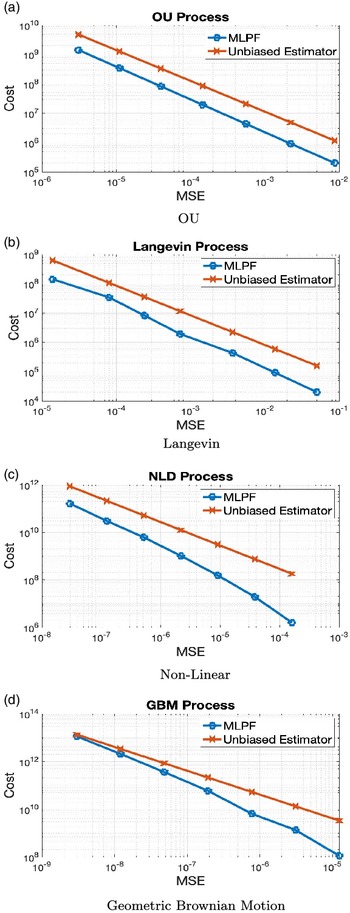
Our results, presented in Figure 1 and Table 1, concern the estimation of the filter at time 100. The average cost ratio (as in Table 1) is the average of the ratio of the cost of (11) to the MLPF at the same MSE levels over the last four (most precise discretization) values which are presented in Figure 1. We also display rate plots (MSE versus cost) for each model, where each plot has two lines in it representing the MLPF estimate calculated at $ L\in\{1,2,{\dots},7\}$ and the associated estimate (11). The plots are all on the $ \log_{10}$ scale.

Figure 1.

Plots of cost against MSE ( $ \log$ – $ \log$ ). The unbiased estimator is in red, and the MLPF estimator is in black.

In Figure 1, for the MLPF algorithm, we expect to see the non-asymptotic rate of $ \frac{\log_{10}(\textrm{Cost})}{\log_{10}(\textrm{MSE})}$ , which will be different from the asymptotic rate owing to the dominating effect of terms that are of order one; as the discretization level l grows, the rate will converge to the asymptotic rate (for instance as in [Reference Jasra, Kamatani, Law and Zhou13]). This effect is present in the simulation results, which show a changing slope (this is more obvious for diffusion models with nonconstant diffusion coefficient) for the line of the MLPF estimator.

We observe from the simulation results that the cost for (11) is higher than the cost for MLPF (the cost ratios range from 3 to 7) at the same MSE level. However, parallel computing could make our estimator more appealing by reducing the actual computing time. We will demonstrate this in our multicore experiments.

4.5. Multicore comparison

We now present our multicore results. We use up to $ 10^3$ MPI cores on the KAUST supercomputer Shaheen to conduct our multicore simulation. We check the parallel speedup and parallel efficiency of the truncated unbiased estimator on the Ornstein–Uhlenbeck process model (with $ Z_{0}=1$ instead) with a specific observation sequence up to time 100. When $ L_{\textrm{max}}=2$ , the truncated unbiased estimator requires $ M \times C = 10^6$ (where C is as discussed in Section 4.2) to achieve variance equal to its squared bias.

Figure 2.

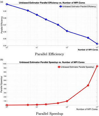
Parallel speedup and parallel efficiency against number of MPI cores for the unbiased estimator.

To demonstrate the parallel scaling power of the truncated unbiased estimator, we use various values of $ M \in \{1,5,10,20,50,100,500,1000\}$ (we fix $ C = 10^3$ ) and record the serial computation time to obtain the estimator on a single core; we also record the parallel computation time on M cores. The parallel speedup is given by the ratio of cost for serial implementation and the cost for parallel implementation, and the parallel efficiency is given by the ratio of parallel speedup and the number of parallel cores.

We compare the parallel speedup and efficiency with number of cores and present their respective semi-log plots in Figure 2. We observe that the parallel speedup scales almost linearly with the number of MPI cores used. This is also validated in the parallel efficiency plot, where we can see the efficiency remains above $ 0.94$ even with $ 10^3$ MPI cores. This demonstrates the parallel power of the unbiased estimator, as it requires no communication among parallel cores during implementation.

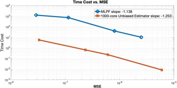
We also compare the performance of the unbiased estimator implemented on $ 10^3$ cores with that of the MLPF on a single core. This is achieved by setting $ M=10^3$ . As illustrated before, parallel implementation of the MLPF offers only a small speedup; thus we do not apply it. We set $ L_{\textrm{max}} \in \{1,2,3,4\}$ for the (1000-core) unbiased estimator and apply the MLPF to obtain similar MSE levels while recording the actual computation time to obtain each estimator. In Figure 3, we present a log–log plot of computation time (in seconds) against the MSE values, for the (1000-core) unbiased estimator and the MLPF. On average we observe that, under the same MSE target, the implementation time of the unbiased estimator is 300 times lower than that of the MLPF.

Figure 3.

Multicore comparison.