1 Introduction
Turbulent flows laden with dense suspensions of particles are common in both natural and industrial settings. Examples include sediment-laden rivers, fluidized bed reactors and slurries produced in manufacturing and agricultural processes. When the fluid is liquid, the particles may be nearly neutrally buoyant but inertial effects can still be important due to the finite size of the particles, resulting in strongly coupled dynamics between the dispersed and continuous phases. The fluid turbulence adds further complexities due to the multi-scale nature of the fluctuations. A practically important case is represented by wall-bounded turbulent flows. These have a hierarchy of scales ranging from the duct/pipe width or boundary layer thickness, to the Kolmogorov and viscous length scales. While particles are typically smaller than the integral/outer scales of the flow, they are often large compared to the viscous/inner scales. This results in complex interactions between the particles and the fluid which are still not completely understood. Here we investigate the two-phase dynamics in a turbulent boundary layer laden with a dense suspension of relatively large particles. We remark that the ‘dense’ (or ‘highly concentrated’) regime can be defined in a number of ways. Following Stickel & Powell (Reference Stickel and Powell2005), we refer to regimes in which one or more of the following conditions occur: the typical inter-particle distance is equal to or smaller than the particle size (i.e. the volume fraction
 $\unicode[STIX]{x1D6F7}=O(10^{-1})$
); particle interaction and lubrication contribute significantly to the suspension rheology; and the rheology is non-Newtonian. Below we briefly review some important results relevant to the present study.
There is substantial evidence that the presence of solid particles can modify fluid turbulence, but the magnitude and even the sign of the change are still debated (Balachandar & Eaton Reference Balachandar and Eaton2010). Gore & Crowe (Reference Gore and Crowe1991) proposed that turbulence is augmented by particles larger than
 $1/10$
of the integral length scale, and attenuated by smaller ones. For a fully developed turbulent boundary layer, this threshold concerns particles significantly larger than the viscous scales. Hetsroni (Reference Hetsroni1989) proposed a criterion based on the particle Reynolds number
 $Re_{p}=U_{slip}D_{p}/\unicode[STIX]{x1D708}$
(
 $D_{p}$
being the particle diameter,
 $\unicode[STIX]{x1D708}$
the kinematic viscosity and
 $U_{slip}$
the slip velocity between both phases), predicting augmented and attenuated turbulence for
 $Re_{p}>400$
and
 $Re_{p}<100$
, respectively. Elghobashi (Reference Elghobashi1994) indicated that turbulence modification occurred when
 $\unicode[STIX]{x1D6F7}$
is higher than approximately
 $10^{-6}$
, although this criterion has been mostly utilized for gas–solid rather than liquid–solid mixtures. Pan & Banerjee (Reference Pan and Banerjee1996) performed simulations of slightly negatively buoyant solid particles in a turbulent liquid channel flow. The particle size was close to the dissipative length scale, and the volume fraction was
 $O(10^{-4})$
. They showed that turbulence was reduced when the particles were smaller than the dissipative length scale and enhanced when the particles were larger. They also showed that the dynamics of the sweep-ejection cycle was modified by the dispersed phase. Modifications to the sweep-ejection cycle by neutrally buoyant finite-size particles was also investigated by Wang, Abbas & Climent (Reference Wang, Abbas and Climent2018) in a slightly turbulent Couette flow and channel flow. Yeo et al. (Reference Yeo, Dong, Climent and Maxey2010) carried out simulations of finite-size particles with positive, negative and neutral buoyancy in homogenous turbulence at
 $\unicode[STIX]{x1D6F7}=6\,\%$
and observed damping of turbulent fluctuations at mid-range wavenumbers, while turbulence at length scales below the particle size was enhanced, indicating that particles facilitate the transfer of energy from large scales to small. Using finite-size neutrally buoyant spheres in a homogeneous turbulent water flow, Bellani et al. (Reference Bellani, Byron, Collignon, Meyer and Variano2012) found that the fluid turbulent kinetic energy was reduced significantly already at volume fractions of 0.14 %, with particles removing energy at the large scales and reinserting it at small scales.
Whether these conclusions hold as the particle size and volume fraction vary, and by which mechanisms the turbulence modulation is realized, is unclear. Studies on dense suspensions of finite-size particles in turbulent flows are sparse, although in recent years novel computational and experimental capabilities have enabled significant progress. Shao, Wu & Yu (Reference Shao, Wu and Yu2012) performed fully resolved direct numerical simulations (DNS) of a horizontal channel flow with both neutrally buoyant and heavy particles up to
 $\unicode[STIX]{x1D6F7}=10\,\%$
. They found that neutrally buoyant particles decreased turbulence near the wall by weakening the intensity of large-scale vortices, while heavy particles settled on the bottom wall and form a rough sediment layer that increased turbulence by shedding vortex structures that propagated into the core region of the channel. Cisse et al. (Reference Cisse, Saw, Gibert, Bodenschatz and Bec2015) considered a von Kármán water flow containing refractive-index-matched neutrally buoyant spheres with diameters approximately
 $1/9$
th of the integral scale of the turbulence. They found that the turbulent kinetic energy suddenly dropped for
 $\unicode[STIX]{x1D6F7}>3\,\%$
, but the inertial-range and small-scale features were unchanged up to
 $\unicode[STIX]{x1D6F7}=10\,\%$
. Wang, Abbas & Climent (Reference Wang, Abbas and Climent2017) numerically investigated a transitional plane Couette flow with finite-size particles up to
 $\unicode[STIX]{x1D6F7}=10\,\%$
. While the particles did not affect the large-scale vortices, they increased the level of turbulent kinetic energy in the smaller scales due to perturbations to the mean flow resulting from the rigidity of the particles. Zhang & Rival (Reference Zhang and Rival2018) measured the effect of particles approximately
 $1/20$
th of the integral scale in decaying turbulence at volume fractions up to 18 %. They showed significant turbulence modulation, which however appeared to saturate at the higher loadings.
In addition to modulating the turbulent fluctuations, particles can modify the bulk effective viscosity. Efforts to characterize the relationship between particle volume fraction
 $\unicode[STIX]{x1D6F7}$
and effective viscosity
 $\unicode[STIX]{x1D707}_{e}$
began with Einstein (Reference Einstein1906), who derived the linear relationship
 $\unicode[STIX]{x1D707}_{e}/\unicode[STIX]{x1D707}=1+(5/2)\unicode[STIX]{x1D6F7}$
for a dilute suspension of rigid and neutrally buoyant spherical particles in a Newtonian fluid (of dynamic viscosity
 $\unicode[STIX]{x1D707}$
) under laminar flow conditions. This estimate was extended by Batchelor & Green (Reference Batchelor and Green1972) for higher volume fractions by deriving a relationship for
 $\unicode[STIX]{x1D707}_{e}/\unicode[STIX]{x1D707}$
that is quadratic in
 $\unicode[STIX]{x1D6F7}$
due to pair-wise hydrodynamic interactions which scale inversely with the square of the distance between particles. For very high volume fractions, the empirical fits given by Eilers (Reference Eilers1941) and Krieger & Dougherty (Reference Krieger and Dougherty1959) have been shown to predict the effective viscosity well in laminar flows (Stickel & Powell Reference Stickel and Powell2005). When the volume fraction approaches the maximum packing limit, the effective viscosity diverges due to the heightened importance of lubrication and contact between particles and the system jams (Sierou & Brady Reference Sierou and Brady2002). The impact of the particle microstructure on the effective viscosity was demonstrated by Yeo & Maxey (Reference Yeo and Maxey2010), who simulated suspensions of negatively buoyant finite-size particles in a laminar Couette flow with volume fractions from 20 to 40 %. They identified different regions with distinct microstructures, including a region of strong particle layering near the wall which produced non-Newtonian effects and increased fluid normal stresses.
The rheological effects become more complex when dealing with regimes where particle inertia cannot be neglected, and standard relationships between volume fraction and effective viscosity are not sufficient to explain the observed behaviour. Bagnold (Reference Bagnold1954) first showed how collisions between particles in the inertial regime could result in shear thickening, where the effective viscosity increases with the shear rate. Matas, Morris & Guazzelli (Reference Matas, Morris and Guazzelli2003) experimentally investigated the effect of a dense suspended phase on the transition to turbulence in pipe flows. For sufficiently large particles, they found a non-monotonic variation of the transitional Reynolds number when increasing
 $\unicode[STIX]{x1D6F7}$
. They also showed that using an effective suspension viscosity did not collapse their results as for a single-phase fluid. Picano et al. (Reference Picano, Breugem, Mitra and Brandt2013) used particle-resolved simulations to show that the effective viscosity increased with the relative strength of the inertial effects, measured by the particle Reynolds number
 $Re_{\unicode[STIX]{x1D6FE}}=\unicode[STIX]{x1D70C}_{f}\dot{\unicode[STIX]{x1D6FE}}a^{2}/\unicode[STIX]{x1D707}$
, where
 $\unicode[STIX]{x1D70C}_{f}$
is the fluid density,
 $\dot{\unicode[STIX]{x1D6FE}}$
is the shear rate and
 $a$
is the particle radius. They termed this behaviour ‘inertial shear thickening’ and showed how inertia modified the particle microstructure and increased the effective excluded volume, resulting in more frequent particle interactions and a sharp increase in effective viscosity. The latter exceeded the prediction of the Eilers’ fit and was not associated with an increase in turbulent stresses, but rather with the additional stresses due to particle–particle interaction. Lashgari et al. (Reference Lashgari, Picano, Breugem and Brandt2014) analysed transition to turbulence in dense regimes with particle volume fractions up to 30 %. They found evidence for inertial shear thickening characterized by a large increase in wall friction with Reynolds number, while the turbulent stresses in the fluid were weakly affected. Picano, Breugem & Brandt (Reference Picano, Breugem and Brandt2015) simulated large, neutrally buoyant particles in a channel flow up to
 $\unicode[STIX]{x1D6F7}=20\,\%$
. They found an overall increase in drag, which at volume fractions less than 10 % was due to augmented turbulent stresses. At higher
 $\unicode[STIX]{x1D6F7}$
they observed reduced turbulent stresses, from which they inferred increased particle-induced stresses and therefore attributed the additional drag to inertial shear thickening. Costa et al. (Reference Costa, Picano, Brandt and Breugem2016) extended this analysis and showed that particle layers near the wall caused the suspension to deviate from the continuum limit, such that the suspension could not be well represented by a bulk effective viscosity in that region. Costa et al. (Reference Costa, Picano, Brandt and Breugem2018) showed that these effects are dependent on particle size: inertial shear thickening is more important when the particle size is large due to the high particle Reynolds number. Zade et al. (Reference Zade, Costa, Fornari, Lundell and Brandt2018) performed experimental measurements of high volume fractions of large spheres in a turbulent square duct for a range of particle sizes, volume fractions and Reynolds numbers using refractive index matched-particle image velocimetry. Depending on Reynolds number, the spheres were either suspended or sedimenting, resulting in different concentration gradients in the vertical direction. They measured a drag increase with the introduction of particles, as well as large reductions in turbulent stresses for high local volume fractions, indicating that the drag increase was due to particle-induced stresses.
As it emerges from this brief review, a unified picture of the complex phenomena that occur in turbulent dense suspensions of large particles is still missing. In particular, experimental observations of the suspension micro-structure, the particle-scale dynamics and the modifications to the fluid phase are lacking, especially for wall-bounded flows. Recent particle-resolved simulations are providing valuable insight, but the achievable Reynolds numbers (and the number of resolvable particles) are still limited. To address this gap, we performed a laboratory investigation of a turbulent open-channel flow in which water is laden with relatively large particles. In order to overcome the challenge of optical access in the dense regime, we use hydrogel spheres of refractive index close to water. This allows the use of optical imaging techniques to measure fluid and particle velocities (Bellani et al. Reference Bellani, Byron, Collignon, Meyer and Variano2012; Byron & Variano Reference Byron and Variano2013; Zade et al. Reference Zade, Costa, Fornari, Lundell and Brandt2018; Zhang & Rival Reference Zhang and Rival2018). The particles are slightly heavier than water and have a diameter of approximately 11 % of the channel depth. Relatively high global volume fractions between 4 and 25 % are investigated, which result in nearly close-packed particle distributions near the wall. We find significant modifications to the mean and root mean square (r.m.s.) velocity fluctuations of the fluid phase at all considered concentrations. By examining the spatial structure of the turbulence and the particle distribution and velocity, we gain insight into the mechanisms by which the particles modify the flow. The paper is organized as follows: in § 2 we describe the experimental set-up, particles and image processing; in § 3 we present the results for the single-phase and particle-laden flow and discuss the particle dynamics and the modification of the flow by particles; and the conclusions are summarized in § 4.
2 Experimental method
2.1 Experimental facility
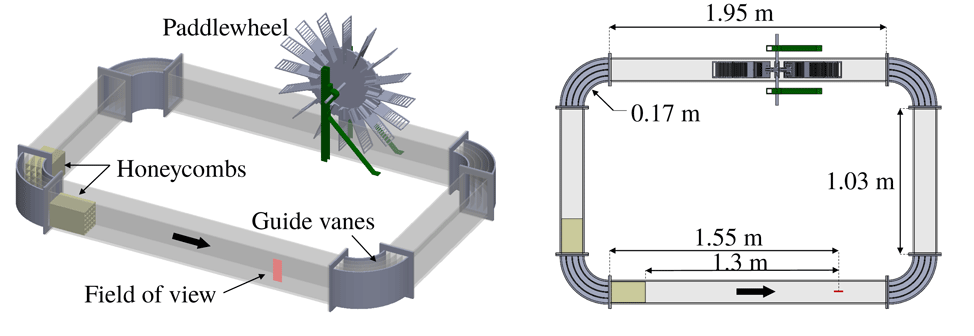
A recirculating open channel with water as the working fluid is used for this experiment. Complete details of the channel design can be found in Adhikari (Reference Adhikari2013) and are just briefly summarized here. The channel walls and floor are made of transparent acrylic. The channel width is 15 cm, with the water filled to a depth
 $H=15~\text{cm}$
. Guide vanes are placed in each of the four corners to reduce secondary flows produced at the turns. The test section is located 1.5 m downstream of a corner, allowing the flow to reach a developed state. A schematic diagram of the channel is shown in figure 1.
Schematic diagram of the water channel showing key components and dimensions. The bold arrow indicates the direction of the flow.

The flow is driven by a paddlewheel with 16 paddles driven by a
 $1/4$
horsepower permanent magnet motor (Leeson, USA) at a constant angular speed of 10 revolutions per minute (RPM). This is used instead of a centrifugal pump or other forcing methods to avoid damaging the hydrogel particles. Standard paddles produce sizeable oscillations, with the fluid velocity rising and falling slightly as they enter and exit the water, partly due to the tangential speed increasing from hub to tip. To reduce these fluctuations and equalize the forcing from the paddle across the channel height, horizontal slots are cut into the paddles whose width increases linearly with the radial distance from the hub. The resulting free-stream velocity is
 $0.21~\text{m}~\text{s}^{-1}$
in the unladen case, which is measured to be constant in time within experimental uncertainty. The power consumed by the paddlewheel is monitored by measuring the voltage and current drawn by the motor.
Because of the size of the hydrogel particles, conventional screens and honeycombs cannot be used to condition the flow. Instead, two custom ‘3D-printed’ honeycombs, 24 cm in length, are placed upstream of the test section to reduce secondary flows. The cells are square with a side length of 4 cm in the first honeycomb and 3 cm in the second honeycomb.
2.2 Particles
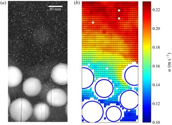
Spherical hydrogel particles (100Candles.com, USA) are used. Their blue tinge results in significant scatter of the illumination light, and they appear as bright circles as shown in figure 2. Their refractive index is nearly matched with water, allowing optical imaging with minor light distortion. The effect on the latter on the measurement accuracy is discussed in § 2.3.
Instantaneous realization of the particle-laden flow. The raw image is shown in (a), where both the large spherical particles and the small flow tracers are visible. The velocity field and detected particles, obtained using the methods described in the text, are shown in (b).

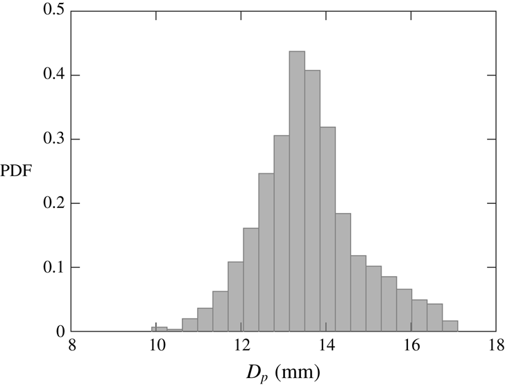
The physical properties of the particles are listed in table 1. The diameter distribution is measured by imaging approximately 850 hydrogel particles placed on a tray in a single layer. Their detection and sizing are performed via a circle-finding function based on the Hough transform. A small number of particles appear not perfectly spherical, which reduces the accuracy of the particle position and diameter estimates. For most particles, however, the major-to-minor axis ratio of the best-fit ellipse is
 ${\leqslant}1.07$
and therefore the effect of non-sphericity on the statistics is deemed negligible. The probability density function (PDF) of the particle diameter is plotted in figure 3.
Properties of the hydrogel particles.
 $D_{p}$
is the mean diameter,
 $D_{p}^{+}$
is the diameter normalized by the viscous length scale of the unladen flow,
 $\unicode[STIX]{x1D70C}_{p}$
is the density,
 $e$
is the coefficient of restitution,
 $V_{t}$
is the terminal velocity,
 $Re_{p,V_{t}}$
is the Reynolds number based on the terminal velocity,
 $m$
is the approximate coefficient of friction for the range of sliding velocities experienced by the particles in this experiment from Cuccia (Reference Cuccia2017),
 $E$
is the elastic modulus and
 $\unicode[STIX]{x1D6F7}_{0}$
is the global volume fraction for the different cases in this study.

Probability density function of hydrogel particle diameters. The standard deviation is 9 % of the mean value.

Vertical position (a) and velocity (b) time series of hydrogel particles dropped from rest in a tank of quiescent water and rebounding off the bottom, averaged over 10 trials.

The terminal velocity
 $V_{t}$
and the coefficient of restitution
 $e$
are measured by dropping individual particles from rest in a large tank of quiescent water and recording 30 f.p.s. videos. Particles are tracked using the same method used for the particle-laden flow measurement, which will be described in the next section. The tank is deep enough (0.3 m) for the particles to reach a steady-state velocity before bouncing off the bottom. The particle position and velocity over time, averaged over 10 trials, are plotted in figure 4. The particle Reynolds number is computed based on the terminal velocity according to
 $Re_{p,V_{t}}=V_{t}D_{p}/\unicode[STIX]{x1D708}$
. The coefficient of restitution
 $e$
is defined as the ratio of a particle’s velocity just after a collision (also averaged over 10 trials) to its velocity before the collision. However, the coefficient of restitution is a function of the particle Stokes number at impact, which varies with the impact velocity (Joseph et al.
Reference Joseph, Zenit, Hunt and Rosenwinkel2001; Gondret, Lance & Petit Reference Gondret, Lance and Petit2002). The characteristic velocity of particle–wall and particle–particle collisions in this experiment is comparable to the particle r.m.s. velocity, which is only approximately 30 % of the particle terminal velocity on average, as will be shown in § 3.3. Therefore, the actual coefficient of restitution of the particle collisions in this experiment will be lower than 0.56. From the results of Joseph et al. (Reference Joseph, Zenit, Hunt and Rosenwinkel2001) and Gondret et al. (Reference Gondret, Lance and Petit2002), we can estimate the reduced value of
 $e$
to be approximately 0.3.
The density of the particles is slightly higher than that of water and was measured in two ways. First, the density was evaluated by directly measuring the mass and volume of several samples of particles: the sample volume is measured using Archimedes’ method, and repeated for six samples of approximately 60 particles each. This measurement was compared with an estimate from the following empirical law for the drag force
 $F_{D}$
on a particle settling at its terminal velocity (Crowe et al.
Reference Crowe, Schwarzkopf, Sommerfeld and Tsuji2011):
 $$\begin{eqnarray}\frac{4F_{D}}{\unicode[STIX]{x03C0}D_{p}^{2}\unicode[STIX]{x1D70C}_{f}V_{t}^{2}}=\frac{12}{Re_{p,V_{t}}}(1+0.15Re_{p,V_{t}}^{0.687}),\end{eqnarray}$$
where
 $F_{D}=\unicode[STIX]{x03C0}D_{p}^{3}g/2$
. From the known terminal velocity and particle Reynolds number, the particle density was calculated and found to differ from the direct measurement by less than 1 %.
The hydrogel particles may deform under pressure. However, the forces experienced by the particles in this experiment are not sufficient to deform them by any visible amount. The deformability of the particles was characterized in a simple uni-axial compression test by measuring the distance
 $\unicode[STIX]{x1D6FF}$
by which a particle is compressed when known amounts of weight ranging from 0.01 to 1 N are applied on top of it. For an elastic sphere compressed between two flat, rigid plates, the relationship between
 $\unicode[STIX]{x1D6FF}$
and the applied force
 $F$
is
 $$\begin{eqnarray}\unicode[STIX]{x1D6FF}=2\left(\frac{9(1-\unicode[STIX]{x1D708}^{2})^{2}}{8D_{p}E^{2}}\right)^{1/3}F^{2/3},\end{eqnarray}$$
where
 $\unicode[STIX]{x1D708}$
here is the Poisson ratio of the material and
 $E$
is the elastic modulus (Lu et al.
Reference Lu, Tung, Hung, Shiau and Hwang2001). Poisson’s ratio was assumed to be 0.5, i.e. the volume of the particle was assumed to remain constant during compression. By fitting a line to
 $\unicode[STIX]{x1D6FF}$
versus
 $F^{2/3}$
measured for a sample of 21 spheres, a value of
 $E=82.7~\text{kPa}$
was obtained.
Because particles are in frequent contact with the wall and other particles in this experiment, the coefficient of friction of the particles may be important as well. Due to their hydrophilic nature, the hydrogel particles are always surrounded by a lubricating layer of water, so their friction coefficient is very low compared to many other materials and is also a function of the sliding velocity. Friction coefficients for polyacrylamide hydrogel spheres sliding on a flat surface of the same material have been measured by Cuccia (Reference Cuccia2017) and were found to be of the order of
 $10^{-2}$
for sliding velocities up to
 $0.1~\text{m}~\text{s}^{-1}$
.
2.3 Fluid velocity measurements
Particle image velocimetry (PIV) is used to measure the velocity of the fluid. The water is seeded with 13-micron silver-coated glass bubbles (Potters Industries) to act as tracers. A 300 W near-infrared pulsed laser with a wavelength of 808 nm (Oxford Lasers, Firefly 300 W) is used for illumination. The laser is positioned above the channel and emits a 1 mm light sheet perpendicular to the channel floor and parallel to the streamwise direction, illuminating a two-dimensional (2-D) measurement plane located at the centreline of the channel. A 15 cm square acrylic plate is fixed at the water surface where the laser sheet enters the water to ensure that the water surface does not distort the laser sheet. Although this results in a shear layer at the surface, the shear layer is sufficiently thin (less than 10 mm thick) that it does not affect our region of interest. Images are captured with a high-speed, 1-megapixel CMOS camera (Phantom, v210) viewing through one of the channel side walls, such that the line of sight is perpendicular to the laser sheet. Each considered case is imaged both with a 50 mm lens, capturing almost 90 % of the channel height, and with a 200 mm lens, zooming on the bottom 3 cm of the channel. The camera frame rate is chosen to obtain typical tracer displacements of 12–14 pixels.
In order to obtain fluid velocity fields, first the pixels belonging to a hydrogel particle image are identified (using the method described in § 2.4) and substituted with Gaussian noise having the same mean and standard deviation as the rest of the corresponding image. This is done so that those pixels do not impose a bias on the PIV cross-correlation. The resulting tracer-only images are used for PIV processing performed with a custom-written software. Because the laser sheet is attenuated by the water and scattered by the particles, the overall brightness of the image decreases slightly from top to bottom. To offset the intensity gradient, a minimum-intensity background subtraction is performed which equalises the light intensity across the image. Multi-pass cross-correlation with an overlap of 50 % between interrogation windows is used to compute fluid displacement fields. Initial interrogation window sizes of 64 by 64 pixels and 128 by 128 pixels are used for the 50 mm lens and 200 mm lens measurements, respectively. A signal-to-noise ratio (SNR) criterion is used to reject spurious velocity vectors. A universal outlier detection criterion (Westerweel & Scarano Reference Westerweel and Scarano2005) is also used to reject vectors that are significantly different from their neighbours. The imaging and PIV processing parameters are summarized in table 2.
Imaging and PIV processing parameters.

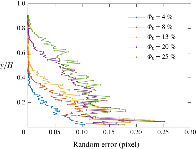
It is verified that the number of images and the length of the recordings are sufficient to reach statistical convergence within the inherent PIV uncertainty. The latter is estimated using the method proposed by Zhang & Rival (Reference Zhang and Rival2018) to account for the decrease in image quality due to the presence of hydrogel particles: the images are shifted by 2 to 16 pixels in the
 $x$
direction, and these known shifts are compared with the displacements calculated by cross-correlation between shifted image pairs. The bias error calculated with this method is found to be negligible (
 ${<}0.05$
pixels), while the random component is plotted in figure 5 as a function of height for the various cases. This is smaller than in the experiments of Zhang & Rival (Reference Zhang and Rival2018) which, however, were conducted under different conditions. The particle size in the present study is much larger, yielding much fewer particle–water interfaces along the illumination path (typically 4–10, versus 45–85 for Zhang & Rival Reference Zhang and Rival2018). Therefore, there is substantially less light distortion and dispersion, and indeed the tracers do not appear statistically larger in the images of the particle-laden cases than in those of the unladen case. Moreover, unlike Zhang & Rival (Reference Zhang and Rival2018), the large hydrogel particles are not contained in the PIV interrogation windows, acting instead as mask for the cross-correlation algorithm. Thus, the number of tracer pairs per interrogation window is not significantly altered, and the impact on the SNR is limited.
Component of the random error in the PIV of the fluid velocity, due to the decreased imaged quality in the presence of the hydrogel particles (see Zhang & Rival Reference Zhang and Rival2018).

Overall, assuming the random error is the main source of inaccuracy leads to uncertainty estimates ranging from 0.9 to 1.9 % for the mean and from 1.7 to 3.7 % for the Reynolds stresses (the larger uncertainties occurring in the more concentrated cases). We note, however, that other potential sources of error due to the particle presence may not be accounted for by the method described above. First, the position of the hydrogel particles with respect to the tracers (and therefore the distortion of the tracer pattern around them) may change between successive frames; this is not captured when comparing shifted images. Second, the masking effect of the hydrogel spheres on the fluid field causes the PIV to under-sample their immediate vicinity. The resulting bias is hard to assess with precision, but its impact is expected to decrease with increasing resolution. The statistics obtained with the 50 mm lens essentially overlap those from the 200 mm lens (the latter having three times higher magnification than the former), suggesting that such bias does not have a major influence on the results or the conclusions drawn from them.
2.4 Particle detection and tracking
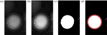
The hydrogel particles are identified and tracked using a custom-written software. To locate the particles, a thresholding method based on the image intensity is used (figure 6). First, a low-pass Gaussian filter with a width of five pixels is applied to the images to smooth away the tracers (figure 6
b). Then, the images are binarized around a threshold intensity corresponding to the minimum brightness of the particles (figure 6
c). The connected groups of bright regions are identified and two conditions are tested: (i) whether the region area
 $A_{i}$
is in the range
 $\unicode[STIX]{x03C0}(0.4D_{p})^{2}<A_{i}<\unicode[STIX]{x03C0}(1.5D_{p})^{2}$
, and (ii) whether its aspect ratio
 $AR_{i}$
is in the range
 $0.93<AR_{i}<1.07$
. If both conditions are satisfied, then the region is identified as a particle (figure 6
d). The coordinates of the particle location are given by the centroid of the region, and the diameter is calculated as the diameter of the equivalent circle with area
 $A_{i}$
.
Threshold method for particle detection used for the near-wall data: (a) original image, (b) low-pass filtered image, (c) binarized image, (d) particle detected.

To find the hydrogel particle velocity, the centroids are tracked between successive image pairs in the time-resolved recordings. First, the local fluid displacement (evaluated from the mean fluid velocity profile interpolated at the wall-normal location of each centroid) is subtracted to the second frame. Then, a nearest-neighbour search with a search radius of one particle diameter is used to match particle centroids in a frame with the shifted centroids in the next one. To obtain particle velocities, the tracks are first smoothed by convolution with a three-point Gaussian kernel; then the streamwise and wall-normal components are differentiated with respect to time. The typical inter-frame displacement is approximately
 $0.2D_{p}$
, and thus the risk of ambiguity in matching particle images is negligible. The method can fail when a particle disappears from one frame to the next, because it exits the field of view or moves out of the laser sheet. In such a case, no velocity vector is found for that particle. We only report the particle velocity up to the height where the number of tracked particles is sufficient to reduce the statistical uncertainty to less than 1 %.
3 Results
3.1 Unladen flow characterization
The unladen flow is first characterized to establish a baseline. Here and in the following, the streamwise and wall-normal coordinates are indicated by
 $x$
and
 $y$
, respectively, and
 $u$
and
 $v$
indicate the respective velocity components. These are Reynolds decomposed as
 $u=\langle u\rangle +u^{\prime }$
and
 $v=\langle v\rangle +v^{\prime }$
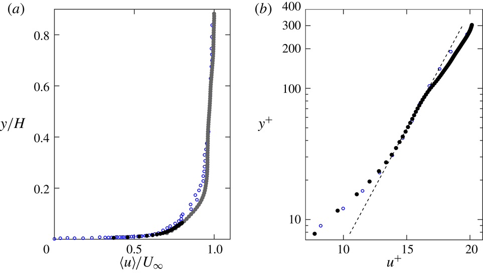
, where angle brackets denote time average and the prime denotes the fluctuating part. As shown in figure 7, the mean velocity profile follows expectations from canonical turbulent boundary layer studies at similar
 $Re_{\unicode[STIX]{x1D703}}$
. The mean velocity profile in outer units (figure 7
a) is compared to the canonical boundary layer of an open-channel flow from Tachie, Bergstrom & Balachandar (Reference Tachie, Bergstrom and Balachandar2003) with a similar
 $Re_{\unicode[STIX]{x1D703}}$
of 1450, showing good agreement. In figure 7(b) a logarithmic law of the form
 $$\begin{eqnarray}u^{+}=\frac{1}{\unicode[STIX]{x1D705}}\ln (y^{+})+B\end{eqnarray}$$
is fit in the range
 $40<y^{+}<90$
. The wall units
 $u^{+}$
and
 $y^{+}$
are defined as
 $u^{+}=u/u_{\unicode[STIX]{x1D70F}}$
and
 $y^{+}=y/\unicode[STIX]{x1D6FF}_{\unicode[STIX]{x1D708}}$
, where
 $u_{\unicode[STIX]{x1D70F}}$
is the friction velocity and
 $\unicode[STIX]{x1D6FF}_{\unicode[STIX]{x1D708}}=\unicode[STIX]{x1D708}/u_{\unicode[STIX]{x1D70F}}$
is the viscous length scale. The von Kármán constant
 $\unicode[STIX]{x1D705}=0.41$
and the additive constant
 $B=5.5$
are used in the log-law fit. The friction velocity is determined by iteratively fitting (3.1) to the mean velocity profile and is found to be
 $u_{\unicode[STIX]{x1D70F}}=9.7~\text{mm}~\text{s}^{-1}$
, while the viscous length scale is found to be 0.1 mm. The profile of the logarithmic layer is compared to the canonical boundary layer of the channel flow from De Graaff & Eaton (Reference De Graaff and Eaton2000) with
 $Re_{\unicode[STIX]{x1D703}}=1430$
, again showing close agreement.
Mean streamwise velocity profile of the unladen flow, in (a) outer units and (b) wall units. Grey and black symbols represent data from the 50 mm lens and 200 mm lens measurements, respectively. The dashed line in (b) indicates the logarithmic law fit. Error bars on the velocity are smaller than the symbol width and are not shown. The profiles are compared with Tachie et al. (Reference Tachie, Bergstrom and Balachandar2003) in (a) and De Graaff & Eaton (Reference De Graaff and Eaton2000) in (b), both shown in blue open circles.

The profiles of Reynolds stresses are shown in figure 8 and are also compared to the boundary layer of De Graaff & Eaton (Reference De Graaff and Eaton2000). The Reynolds stress profiles are similar to canonical expectations at this
 $Re_{\unicode[STIX]{x1D703}}$
, with some discrepancies in the locations and magnitudes of the peak stresses. These are likely due to the non-canonical features of the channel design (honeycombs with a very large cell size, unconventional forcing and limited channel width), and possibly to insufficient spatial resolution. As the unladen flow mostly provides a basis for comparison with the particle-laden cases, minor departures from canonical conditions are not concerning. Physical parameters of the water channel and the unladen boundary layer properties are reported in table 3.
Physical parameters of the water channel and unladen boundary layer properties.
 $U_{\infty }$
is the free-stream velocity,
 $\overline{U}$
is the depth-averaged velocity,
 $H$
is the water depth,
 $w$
is the channel width,
 $\unicode[STIX]{x1D6FF}_{99}$
is the boundary layer thickness and
 $u_{\unicode[STIX]{x1D70F}}$
is the friction velocity. The depth-averaged velocity is defined as
 $\overline{U}=1/H\int _{0}^{H}u(y)\,\text{d}y$
, the boundary thickness is defined such that
 $u(\unicode[STIX]{x1D6FF}_{99})=0.99U_{\infty }$
and the friction velocity is determined by fitting (3.1) to the mean fluid velocity profile.
 $Re_{b}=\overline{U}H/\unicode[STIX]{x1D708}$
,
 $Re_{\unicode[STIX]{x1D70F}}=u_{\unicode[STIX]{x1D70F}}\unicode[STIX]{x1D6FF}_{99}/\unicode[STIX]{x1D708}$
and
 $Re_{\unicode[STIX]{x1D703}}=U_{\infty }\unicode[STIX]{x1D703}/\unicode[STIX]{x1D708}$
are the depth-averaged, friction and momentum thickness Reynolds numbers, respectively. Standard water properties at
 $22\,^{\circ }\text{C}$
are used in the calculations.

Profiles of streamwise turbulent normal stress (a), wall-normal normal stress (b) and shear stress (c) of the unladen fluid in wall units. Grey and black symbols represent data from full-channel imaging and near-wall imaging, respectively. Error bars on the velocity are smaller than the symbol width and are not shown. The profiles are compared with De Graaff & Eaton (Reference De Graaff and Eaton2000) shown in blue open circles.

3.2 Particle spatial distribution
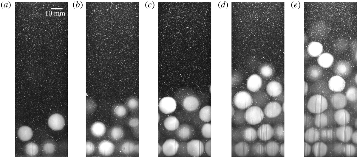
Figure 9 shows sample raw images for the different volume fractions considered, highlighting the tendency of the spheres to concentrate in the bottom part of the channel flow and form layers. To quantitatively characterize the spatial distribution of particles we first examine the wall-normal profile of the time-averaged local volume fraction. Because the latter displays strong variations in the wall-normal coordinate, in the following we indicate it as
 $\unicode[STIX]{x1D6F7}$
, while the global (depth- and time-averaged) volume fraction is denoted as
 $\unicode[STIX]{x1D6F7}_{0}$
. To avoid errors due to particle under-detection, the area occupied by particles is defined for this calculation as the area of the low-pass filtered images exceeding the particle brightness threshold (the blank area of figure 6
c). That the area fraction of particles on an intersecting plane is equivalent to the volume fraction is an established result in stereology (Underwood Reference Underwood1969). While using the area fraction of particles intersected by the centreline plane to estimate volume fraction does not account for side wall effects, these effects are expected to be negligible due to the gravitational settling of the particles, which distributes them fairly evenly in the spanwise direction within the channel (as confirmed by visual inspection). Estimates of the global volume fraction based on this method are in close agreement with the values based on the amount of particles used in each experiment, differing by at most 10 %.
Sample raw images of the particle-laden cases: (a)
 $\unicode[STIX]{x1D6F7}_{0}=4\,\%$
, (b)
 $\unicode[STIX]{x1D6F7}_{0}=8\,\%$
, (c)
 $\unicode[STIX]{x1D6F7}_{0}=13\,\%$
, (d)
 $\unicode[STIX]{x1D6F7}_{0}=20\,\%$
and (e)
 $\unicode[STIX]{x1D6F7}_{0}=25\,\%$
.

The mean volume fraction profiles are plotted in figure 10 for the different
 $\unicode[STIX]{x1D6F7}_{0}$
. When particles are added to the flow, a concentration gradient develops from the wall to the free surface due to their negative buoyancy. The dense horizontal layers produce peaks in the volume fraction profiles. Note that
 $\unicode[STIX]{x1D6F7}$
can exceed the maximum packing fraction because it is sampled over wall-normal bins that are narrower than the particle diameter. The layering becomes stronger with higher
 $\unicode[STIX]{x1D6F7}_{0}$
, and for the densest cases the volume fraction within the first particle layer approaches the packing limit. The peak local volume fraction in the first particle layer does not increase monotonically with
 $\unicode[STIX]{x1D6F7}_{0}$
, for which a physical explanation is not clear. However, the non-monotonicity is only manifest in the closely packed particle layers of the two highest
 $\unicode[STIX]{x1D6F7}_{0}$
cases, where local concentration measurement may suffer from increased uncertainty due to limitations of the imaging method.
Shao et al. (Reference Shao, Wu and Yu2012) observed a similar layering effect for large particles much heavier than the fluid phase. Other researchers found that a similar layering along the wall can occur even when the particles are perfectly neutrally buoyant (Picano et al. Reference Picano, Breugem and Brandt2015; Costa et al. Reference Costa, Picano, Brandt and Breugem2016, Reference Costa, Picano, Brandt and Breugem2018; Wang et al. Reference Wang, Abbas and Climent2017), due to a confinement/excluded volume effect: particles that are transported to the wall become trapped there by a combination of lubrication with the wall and collisions with other particles outside the layer. Successive layers can form when particles become trapped between a stable near-wall particle layer and collisions from particles farther from the wall. In our experiment, particle layering is due to both gravitational and confinement effects. Such effects were also observed experimentally by Zade et al. (Reference Zade, Costa, Fornari, Lundell and Brandt2018).
Profiles of mean local volume fraction for the particle-laden cases.

To investigate the spatial distribution of the particles in the streamwise direction, the spatial autocorrelation of the local particle concentration is calculated. For this purpose, the pixel intensity is used as a proxy for the concentration. A moving-average filter with a width of five pixels is applied to the images. Horizontal bands in the lower part of the images are considered, each approximately 15 mm or 86 pixels thick and roughly capturing one particle layer. The bands in successive images are stitched together using an approach similar to Taylor’s hypothesis, with the band-averaged particle velocity playing the role of the convection velocity. Finally, the spatial autocorrelation of intensity
 $r_{i}$
is calculated for the
 $i$
th band as:
 $$\begin{eqnarray}r_{i}(\unicode[STIX]{x0394}x)=\frac{1}{y_{i+1}-y_{i}}\int _{y_{i}}^{y_{i+1}}\frac{\langle I^{\prime }(x,y)I^{\prime }(x+\unicode[STIX]{x0394}x,y)\rangle }{\langle I^{\prime }(x,y)^{2}\rangle }\,\text{d}y,\end{eqnarray}$$
where
 $I^{\prime }=I-\langle I\rangle$
is the image intensity after subtracting the mean value, and
 $y_{i}$
and
 $y_{i+1}$
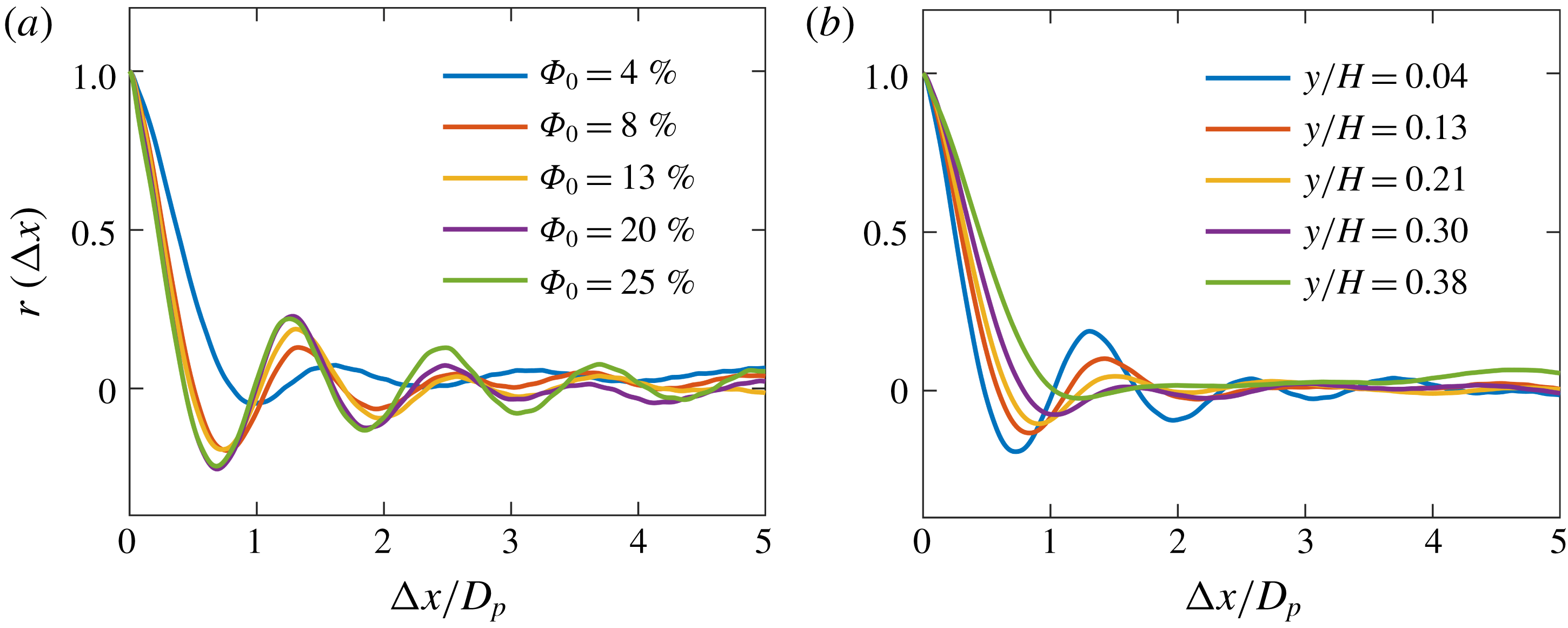
are the lower and upper wall-normal limits of each band, respectively. The autocorrelation is compared between different volume fractions in the lowest particle layer (figure 11
a), and between the different layers for the representative
 $\unicode[STIX]{x1D6F7}_{0}=13\,\%$
case (figure 11
b). The series of peaks in the autocorrelation provide insight on the particle microstructure. The separation between peaks corresponds to the mean streamwise interparticle spacing. For particles of a given size, the magnitude and width of the peaks indicate how regular the interparticle spacing is: peaks with a relatively large magnitude and narrow width indicate that the particles are very regularly spaced, while peaks with a smaller magnitude and a greater width correspond to more variable spacing. The mean interparticle spacing in the dense regions varies between 1.2 and 1.8 particle diameters, increasing with decreasing volume fraction. As noted above, in the lower layers of the higher
 $\unicode[STIX]{x1D6F7}_{0}$
cases, the particles reach a nearly close-packed configuration with a small interparticle gap, indicated by relatively tall, narrow peaks separated by slightly more than one particle diameter.
Spatial autocorrelations of instantaneous particle concentration. The autocorrelation is compared between (a) different volume fractions in the bottom particle layer (
 $y/H=0.04$
), and (b) different wall-normal locations for the
 $\unicode[STIX]{x1D6F7}_{0}=13\,\%$
case. The five wall-normal coordinates, when normalized by the particle diameter, are approximately
 $y/D_{p}=0.5$
, 1.5, 2.5, 3.5 and 4.5.
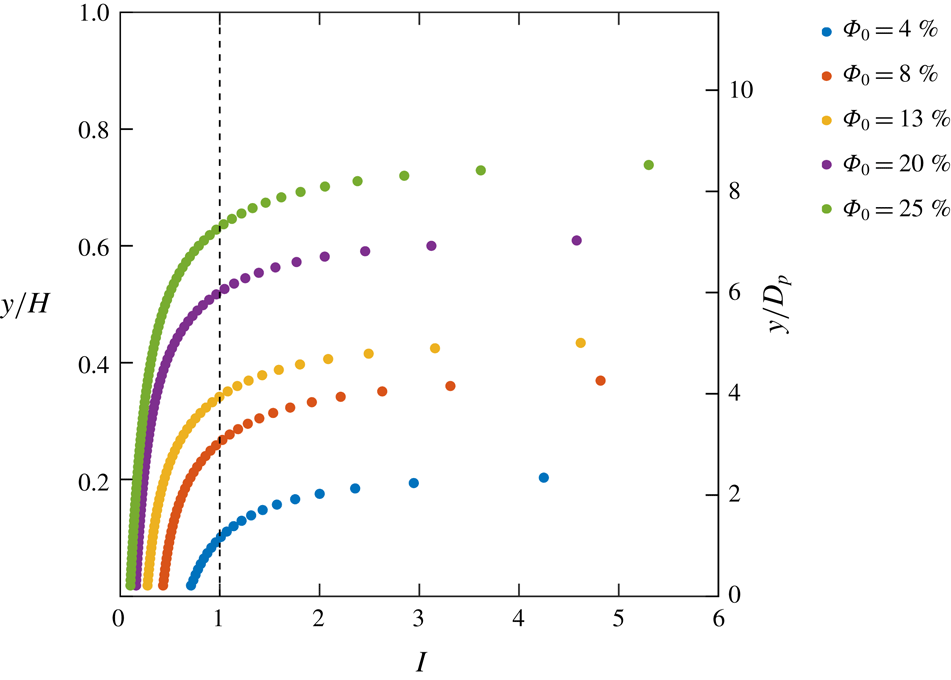
Although the particles are only slightly negatively buoyant, they are still very inertial due to their large size. To describe the particle dynamics quantitatively, the inertial number was computed. This is used in rheology to compare the ratio of inertial forces to confining forces in dense granular flows (e.g. Da Cruz et al. Reference Da Cruz, Emam, Prochnow, Roux and Chevoir2005) and is given by:
 $$\begin{eqnarray}I=\frac{D_{p}|\text{d}\langle u\rangle /\text{d}y|}{\sqrt{P_{p}/\unicode[STIX]{x1D70C}_{p}}},\end{eqnarray}$$
where
 $P_{p}$
is the particulate pressure representing the normal stress associated with particle interactions (Revil-Baudard et al.
Reference Revil-Baudard, Chauchat, Hurther and Barraud2015), given by:
 $$\begin{eqnarray}P_{p}=\left\{\begin{array}{@{}ll@{}}0\quad & \text{for }y>y_{c}\\ (\unicode[STIX]{x1D70C}_{p}-\unicode[STIX]{x1D70C}_{f})g\displaystyle \int _{0}^{y_{c}}\unicode[STIX]{x1D6F7}(y)\,\text{d}y\quad & \text{otherwise,}\end{array}\right.\end{eqnarray}$$
where
 $y_{c}$
is the wall-normal coordinate at which
 $\unicode[STIX]{x1D6F7}=\unicode[STIX]{x1D6F7}_{c}$
, that is the critical volume fraction above which interparticle stresses cannot be neglected. Following Hsu, Jenkins & Liu (Reference Hsu, Jenkins and Liu2004) and Revil-Baudard et al. (Reference Revil-Baudard, Chauchat, Hurther and Barraud2015), we choose the critical volume fraction as corresponding to an interparticle spacing of one particle diameter, i.e. a centre-to-centre interparticle distance
 $l_{c}=2D_{p}$
, yielding
 $\unicode[STIX]{x1D6F7}_{c}=\unicode[STIX]{x03C0}D_{p}^{3}/(6l_{c}^{3})=\unicode[STIX]{x03C0}/48\approx 7\,\%$
. The measured volume fraction profiles are fit with a logistic function in order to obtain a coarse-grained concentration gradient. To avoid amplifying noise in the data, the profiles of mean velocity are also fit with a second-order polynomial. The vertical profiles of inertial number are shown in figure 12. An inertial number
 $I\approx 0$
corresponds to a quasi-static, solid-like regime.
 $I\gtrsim 1$
corresponds to a ‘gaseous’ regime (Forterre & Pouliquen Reference Forterre and Pouliquen2008) where binary particle collisions dominate the dynamics. Intermediate values correspond to a liquid-like, contact-dominated regime in which both frictional and collisional interactions are important. The near-wall regions of the
 $\unicode[STIX]{x1D6F7}_{0}=20\,\%$
and 25 % cases approach the solid-like regime, although there is no bedform in the present flow, so the particles are never in stasis. The position for which
 $I\approx 1$
represents an approximate boundary between the frictional and collisional regimes. The wall-normal height of this transition increases with global volume fraction, the contact-dominated regime extending through nearly two thirds of the channel in the
 $\unicode[STIX]{x1D6F7}_{0}=25\,\%$
case. In the next subsections, the influence of the high inertial number on the particle–fluid dynamics will be discussed.
Profiles of inertial number for the different volume fraction cases. The vertical dashed line shows the location of
 $I=1$
where the dynamics transitions from frictional to collisional.

3.3 Single-point statistics of fluid and particle velocity
The mean fluid velocity profiles for the five volume fraction cases are shown in figure 13 and compared with the unladen case. These, as all other fluid statistics, are computed using only points located around the particles; no attempt is made to interpolate the fluid velocity at the particle locations. The addition of particles has a dramatic effect on the mean velocity profiles: the fluid velocity is strongly reduced near the wall and is greatly increased in the outer region. The overall consequence is a positive mean shear across most of the channel height. (The profiles do knee towards the top of the channel, where negligible shear stress exists. The topmost measurements suffer from reflections from the water surface and are not plotted.) The local velocity gradient near the wall is strongly reduced as well. These effects are stronger for higher volume fractions. The depth-averaged velocity obtained by averaging the wall-normal profile is similar (within 3 %) for all cases.
Mean fluid streamwise velocity profiles. The velocities are normalized by the free-stream velocity of the unladen case,
 $U_{\infty ,0}$
.

Reduced streamwise velocities near the wall have been previously observed by Picano et al. (Reference Picano, Breugem and Brandt2015). They attributed this to increased turbulent fluctuations when
 $\unicode[STIX]{x1D6F7}_{0}<10\,\%$
and to inertial shear thickening when
 $\unicode[STIX]{x1D6F7}_{0}>10\,\%$
. Inertial shear thickening is a possible explanation also for the reduced near-wall velocity in our experiment. While we cannot experimentally evaluate the particle stresses as defined by Zhang & Prosperetti (Reference Zhang and Prosperetti2010) and Picano et al. (Reference Picano, Breugem and Brandt2015), we can reason as follows. The paddlewheel rotates at a constant speed, and by measuring the voltage and current drawn by the motor, we find that the power consumed by the paddlewheel increases by less than 7 % from the unladen case to the
 $\unicode[STIX]{x1D6F7}_{0}=25\,\%$
case. Assuming that the mechanical efficiency is roughly constant, this indicates that the rate of work done on the fluid by the paddlewheel also increases by less than 7 %. Equating the rate of work done by the paddlewheel
 ${\dot{W}}$
to the dissipation on the channel walls, it can be shown that the wall friction (quantified by the friction velocity
 $u_{\unicode[STIX]{x1D70F}}$
) varies with
 ${\dot{W}}^{1/4}$
, so the wall friction is expected to increase by only 1 % from the unladen to the
 $\unicode[STIX]{x1D6F7}_{0}=25\,\%$
case. Because the fluid stress at the wall is essentially unchanged in all cases, the reduced near-wall velocity gradient implies an increase in effective viscosity with increasing
 $\unicode[STIX]{x1D6F7}_{0}$
. Later in this section, it will be shown that this is not associated with larger Reynolds stresses close to the wall. Therefore, the increase in effective viscosity is rather attributable to particle-induced stresses.
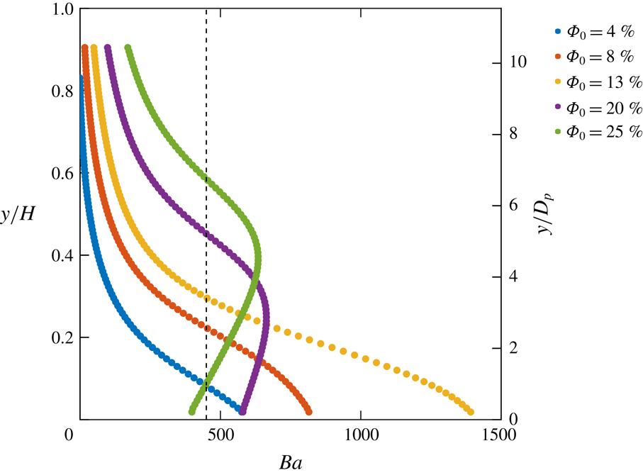
While one may attempt to describe the bulk rheology of the mixture, the discrete layering of the particles results in non-continuum dynamics (Costa et al. Reference Costa, Picano, Brandt and Breugem2016), which is manifest in the dips of the mean fluid velocity profile (figure 13) corresponding to the particle layers. Therefore, the mechanism of inertial shear thickening appears somewhat modified. Over a large fraction of the channel, particle layers slide over each other and experience friction from contact with the adjacent layers. The latter also affect the carrier fluid flow through the momentum coupling between particles and water. This may be viewed as a specific type of particle-induced stress, resulting in an increased effective viscosity. Such effect is usually quantified by the Bagnold number (Bagnold Reference Bagnold1954), i.e. the ratio of particle collision stresses to viscous fluid stresses:
 $$\begin{eqnarray}Ba=\frac{\unicode[STIX]{x1D70C}_{p}D_{p}^{2}\unicode[STIX]{x1D706}^{1/2}}{\unicode[STIX]{x1D707}}\frac{\text{d}\langle u\rangle }{\text{d}y},\end{eqnarray}$$
where the typical interparticle distance is estimated as:
 $$\begin{eqnarray}\unicode[STIX]{x1D706}=\frac{1}{\left({\displaystyle \frac{\unicode[STIX]{x1D6F7}_{max}}{\unicode[STIX]{x1D6F7}_{0}}}\right)^{1/3}-1}\end{eqnarray}$$
and where the maximum packing fraction is set to
 $\unicode[STIX]{x1D6F7}_{max}=0.74$
.
 $Ba<40$
corresponds to a macro-viscous regime (typical of low Reynolds numbers and low volume fractions) where stress and shear rate are linearly related, while
 $Ba>450$
corresponds to a grain-inertia regime where collision stresses dominate. Profiles of
 $Ba$
for the present cases range are shown in figure 14, calculated using a logistic fit of local volume fraction and a second-degree polynomial fit of the fluid velocity to obtain coarse-grained estimates. In the near-wall particle layers,
 $Ba$
is found to be well into the grain-inertia regime in all cases, which is consistent with the presence of dips in the fluid velocity profiles corresponding to the peaks in local volume fraction. The one exception is very near the wall in the highest volume fraction case, where the dynamics is approaching the quasi-static regime as seen in the previous section. This shows that the collisional and frictional dynamics between particle layers is an important factor in determining the fluid velocity profiles.
Profiles of Bagnold number for the different volume fraction cases. The vertical dashed line shows the location of
 $Ba=450$
above which the dynamics transitions to the grain-inertia regime.

Next, we analyse the mean fluid velocity profiles to determine whether they contain a region that follows a logarithmic law of the form (3.1). For a particle-laden channel flow, Picano et al. (Reference Picano, Breugem and Brandt2015) observed the presence of a log region up to
 $\unicode[STIX]{x1D6F7}_{0}=20\,\%$
; however, the values of
 $\unicode[STIX]{x1D705}$
and
 $B$
were significantly modified compared to the unladen case, both decreasing with volume fraction. In our experiment, the log-law constants
 $\unicode[STIX]{x1D705}$
and
 $B$
and the friction velocity
 $u_{\unicode[STIX]{x1D70F}}$
are all unknown in the particle-laden cases:
 $u_{\unicode[STIX]{x1D70F}}$
cannot be measured directly due to the limited spatial resolution, nor can it be calculated a priori as standard estimates for
 $u_{\unicode[STIX]{x1D70F}}$
do not apply. However, as discussed earlier,
 $u_{\unicode[STIX]{x1D70F}}$
is expected to undergo a negligible increase from the unladen to the
 $\unicode[STIX]{x1D6F7}_{0}=25\,\%$
case. Thus, the friction velocity of the unladen flow,
 $u_{\unicode[STIX]{x1D70F},0}$
, is used as scaling unit for the particle-laden cases.
In figure 15 a least-squares regression line is fit in the region
 $40<y^{+,0}<90$
(where the superscript emphasizes the use of the wall units derived from the unladen flow). A logarithmic region can clearly be seen for all cases in the compensated mean velocity profiles. The vertical dashed lines correspond to the locations of the first two particle layers, as determined from the peaks in the local volume fraction profiles. The entire log region is contained within the first particle layer. This may explain why a logarithm behaviour is recovered at all in the present case. The classic scaling argument derives the log law in the region where
 $y$
is large compared to the viscous scales and small compared to the outer scales (Pope Reference Pope2000). Similarly, here a logarithmic behaviour is recovered with a vertical extent that remains largely unchanged with the addition of particles because the particle diameter is much larger than the viscous length scale.
Compensated mean streamwise velocity profiles in single-phase wall units showing the existence of a logarithmic region in all cases (horizontal dashed line). The vertical dashed lines indicate the location of the first two particle layers. The superscript 0 indicates the use of single-phase wall units.

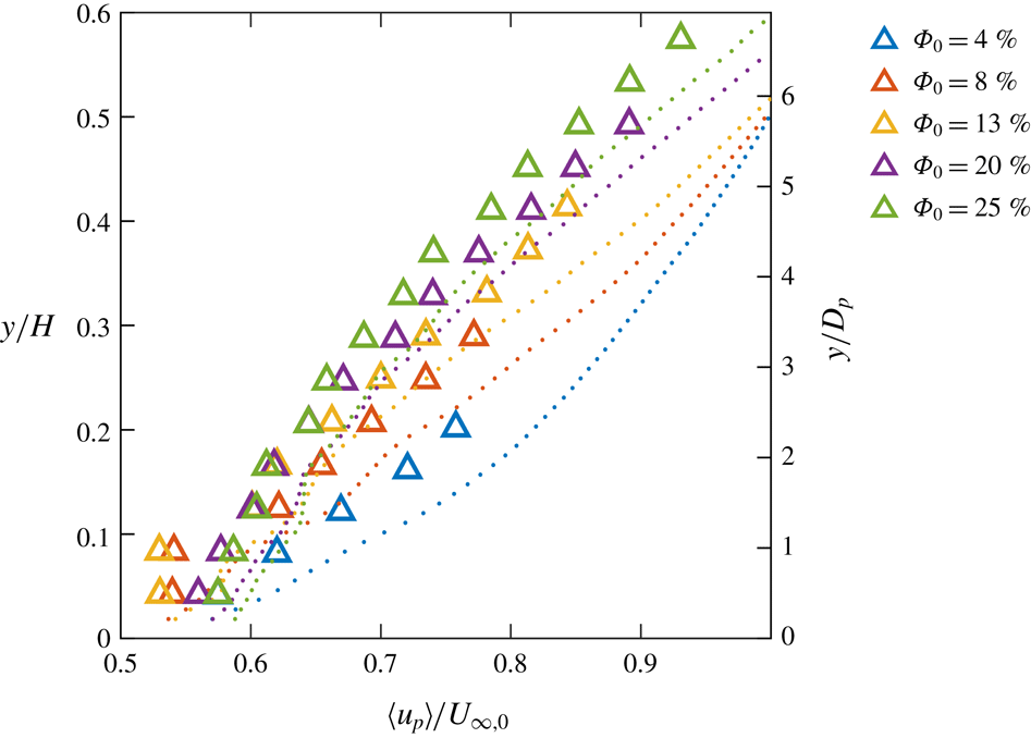
The mean particle velocity profiles are compared to the mean fluid velocity profiles in figure 16. It is observed that the particles consistently lag the fluid at all heights. This is in keeping with the view that the particle layers experience significant friction as they slide over each other. Indeed, for the
 $\unicode[STIX]{x1D6F7}_{0}=20\,\%$
and 25 % cases, the two particle layers closest to the wall move at approximately the same speed, suggesting that the friction between them is larger than the friction between the lower layer and the wall. The shape of the particle velocity profiles is similar to the corresponding fluid velocity profiles. This is especially apparent in the high volume fraction cases, for which particle statistics are measured over most of the boundary layer thickness. The drag exerted by the particles inhibits the fluid flow, especially near the wall where the volume fraction is higher and the particles leave a clear footprint on the fluid profiles.
Mean particle velocity profiles (triangles) compared with the mean fluid velocity profiles (dots). The velocities are normalized by the free-stream velocity of the unladen case.

Previous studies concerned with neutrally buoyant spheres in wall-bounded turbulence reported particles moving at roughly the same speed as, and in fact somewhat faster than, the carrier fluid (Picano et al.
Reference Picano, Breugem and Brandt2015; Costa et al.
Reference Costa, Picano, Brandt and Breugem2016, Reference Costa, Picano, Brandt and Breugem2018). It may seem surprising that a 0.7 % excess in particle density over the fluid density results in such a large change of relative velocity. However, negative buoyancy determines a sizeable terminal velocity of our relatively large hydrogel spheres, in fact comparable to the fluid velocity fluctuations and with a correspondingly elevated
 $Re_{p,V_{t}}$
(table 1). This in turn leads to the strong (and consequential) multi-layer stratification discussed in § 3.2. In comparison, Picano et al. (Reference Picano, Breugem and Brandt2015) and Costa et al. (Reference Costa, Picano, Brandt and Breugem2016, Reference Costa, Picano, Brandt and Breugem2018) found clear evidence of only one layer in the concentration profile (although Costa et al. (Reference Costa, Picano, Brandt and Breugem2018) showed near-wall inhomogeneities at distances proportional to the particle diameter up to
 $y/D_{p}=4$
). Indeed, according to Costa et al. (Reference Costa, Picano, Brandt and Breugem2016) the neutrally buoyant particle case admits a distinction between a near-wall layer and the bulk region, the latter being amenable to an effective-viscosity-based description. In our case we cannot directly evaluate
 $\unicode[STIX]{x1D707}_{e}$
, but the dramatic change in the shape of the velocity profiles indicate that a simple collapse is not attainable. The qualitative difference is rooted in the role of gravity, that pushes the particles towards the wall and against each other. This not only results in higher concentrations, but in more frequent and continuous contact, enhancing the importance of friction with respect to the neutrally buoyant particle case (Costa et al.
Reference Costa, Picano, Brandt and Breugem2018).
For a more quantitative insight on the particle inertia, the slip velocity between particles and fluid is presented in figure 17(a) in terms of the slip particles Reynolds number,
 $Re_{slip}=(\langle u\rangle -\langle u_{p}\rangle )D_{p}/\unicode[STIX]{x1D708}$
. Notice that this definition returns positive values for particles lagging the fluid. The values of
 $Re_{slip}$
are well in the wake-shedding regime, although they generally decrease with increasing
 $\unicode[STIX]{x1D6F7}_{0}$
: with gravity, the closely packed particles offer high resistance to the fluid flow, slowing it down and reducing the fluid–particle slip. Indeed, despite some experimental scatter, the slip velocities show local maxima at heights falling in between the dense layers. Note that the particle tracking measures translational velocity only, not rotation, so the slip velocity calculated here may slightly overestimate the slip velocity actually felt by the particle. Figure 17(b) presents the particle Reynolds number based on the local shear rate
 $\text{d}\langle u\rangle /\text{d}y$
, evaluated by differentiating the second-order polynomial fit. This is preferred to a global definition of
 $\dot{\unicode[STIX]{x1D6FE}}$
such as
 $U_{\infty }/H$
, which does not capture the variation of shear across the boundary layer and between the different cases. The relatively large values, e.g. compared to Picano et al. (Reference Picano, Breugem, Mitra and Brandt2013), confirm the strongly inertial particle dynamics. The near-wall values of
 $Re_{\unicode[STIX]{x1D6FE}}$
, like for
 $Re_{slip}$
, also decrease with increasing
 $\unicode[STIX]{x1D6F7}_{0}$
: the highly concentrated particles experience frequent frictional contact, resulting in inhibited relative motion of the adjacent layers and less steep gradients in the particle velocity profiles; the coupling with the fluid flow causes then a reduced shear. The evolution of the fluid profiles with wall distance leads to an inverted trend away from the wall, but at locations where the particle concentration is relatively low.
Profiles of particle Reynolds number based on (a) the local slip velocity and (b) local shear rate.

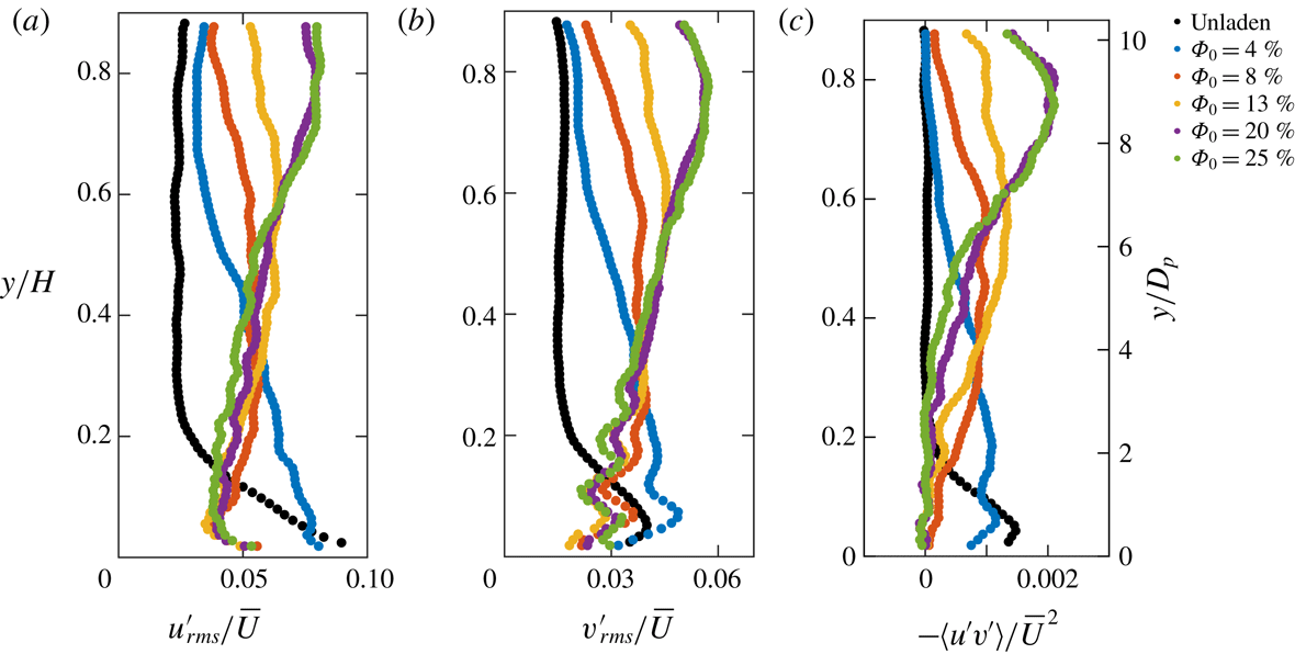
Profiles of streamwise and wall-normal r.m.s. fluid velocity fluctuations and Reynolds shear stresses are presented in figure 18. Again, the signatures of the particle layers are visible on the fluid statistics. In general, the particles reduce turbulent fluctuations near the wall, but greatly increase them away from the wall. The stresses reach a maximum that moves away from the wall with increasing
 $\unicode[STIX]{x1D6F7}_{0}$
, occurring at distances where the local volume fraction is typically small. To confirm how the addition of particles alters the production of turbulence, the shear production profile
 $$\begin{eqnarray}P=-\frac{\text{d}\langle u\rangle }{\text{d}y}\langle u^{\prime }v^{\prime }\rangle\end{eqnarray}$$
is plotted for each volume fraction case (figure 19). A second-order polynomial is fit to the velocity profile before taking its derivative to avoid amplifying noise in the data. In the presence of particles, shear production is strongly damped near the wall compared to the unladen case, and the damping is stronger for higher
 $\unicode[STIX]{x1D6F7}_{0}$
.
Profiles of the fluid streamwise (a) and wall-normal (b) r.m.s. velocity fluctuations and Reynolds shear stresses (c), normalized by the depth-averaged velocity.

Profiles of shear production normalized by the depth-averaged velocity and the channel height.

Profiles of streamwise (a) and wall-normal (b) r.m.s. velocity fluctuations of the particles (triangles) compared to the fluid (dots).

This modification of the vertical structure suggests that the particles are mechanically damping turbulence where the local volume fraction is high: fluid velocity fluctuations are quenched by viscous dissipation on the surface of particles, disrupting turbulent structures as they form. In this region the particles are in the ‘gaseous regime’ and are relatively free to move and shed wakes (given the range of
 $Re_{slip}$
discussed above). However, the local particle presence is not sufficient to explain the intense turbulence activity in the outer region. This is rather attributable to the high shear-driven turbulence production above the particle-dense layers. The large mean shear throughout the channel height (due to the layering behaviour of the particles and the friction between layers) greatly amplifies the shear production, which is maximum in regions of the channel with very sparse particles. A similar remark was made by Shao et al. (Reference Shao, Wu and Yu2012) in their simulations of channel flow laden by heavy particles, where they also observed eddies ascending and propagating unobstructed through the core region. These results are also consistent with the square duct experiments of Zade et al. (Reference Zade, Costa, Fornari, Lundell and Brandt2018) in their large, sedimenting particle case, in which they found strong suppression of turbulent fluctuations near the bottom wall and strong enhancement in the particle-sparse upper region.
The streamwise and wall-normal r.m.s. of the particle velocity fluctuations (
 $u_{p,rms}$
and
 $v_{p,rms}$
, respectively) are calculated and compared to that of the fluid in figure 20. The magnitude of the streamwise component is almost constant with height. This may be due to the fact that the streamwise fluctuations are mostly caused by inter-particle collisions, and this dynamics is weakly affected by the wall distance. In contrast, the presence of the wall itself attenuates
 $v_{p,rms}$
in its vicinity. These trends are quantitatively similar to the respective fluid fluctuations. Given the large particle inertia, this similarity appears as an effect of the particles imposing their behaviour on the fluid, as discussed previously for the mean flow. In summary, the tendency of the particles to align in layers, and the consequent mean shear imposed on the fluid flow, result in large shear production which in turn leads to the enormously increased fluid fluctuations far from the wall.
However, an exception to the trend is observed for the
 $\unicode[STIX]{x1D6F7}_{0}=4\,\%$
case. In this case, there is significant shear production and turbulent energy in the fluid near the wall, compared to the higher volume fraction cases, even exceeding that the of the unladen flow. Also in this case, the particle and fluid streamwise fluctuations are of the same magnitude. As the volume fraction increases,
 $u_{rms}$
decreases while
 $u_{p,rms}$
does not show a clear trend. This indicates that particles augment the fluid turbulence when the volume fraction is moderate, while they attenuate it in the denser conditions. This is qualitatively consistent with the results of Picano et al. (Reference Picano, Breugem and Brandt2015) for neutrally buoyant particles. They found that turbulent fluctuations were augmented for lower volume fractions and attenuated for higher volume fractions, with the transition occurring around
 $\unicode[STIX]{x1D6F7}_{0}=10\,\%$
. Again, our case is significantly different due to the much stronger stratification caused by gravity. The threshold for such transition is likely to be problem dependent.
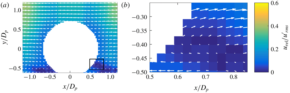
To investigate possible modality of energy transfer from particles to fluid, it is useful to consider the average flow topology around a particle. Specifically, we compute the particle-centred mean relative velocity field for the
 $i$
th particle:
 $u_{rel,i}(x,y)=u(x,y)-u_{p,i}$
. The mean field is obtained by ensemble averaging over all particles within a specific region. In figure 21 we present the
 $\unicode[STIX]{x1D6F7}_{0}=4\,\%$
case in the near-wall region corresponding to the first particle layer (the higher layers do not contain enough particles to obtain converged statistics). Only particles that are not in direct contact with any others in the field of view are included in the average. This yields a set of 715 particles used in the bottom layer. As mentioned, the particle Reynolds number based on the slip velocity is in the wake-shedding regime. Indeed, in the mean relative velocity field a marked velocity deficit can be seen in front of the particle (that is the wake region, since the particles are lagging the fluid). A detailed view in the inset (figure 21
b) highlights the flow field in the velocity deficit region, where a recirculation zone is observable. This feature likely participates in the near-wall production of turbulent fluctuations.
The particle-centred mean relative velocity field, in particle-centred coordinates, for particles from the
 $\unicode[STIX]{x1D6F7}_{0}=4\,\%$
case whose wall-normal position is in the range
 $0<y/D_{p}<1.2$
, and (b) detailed view of the region indicated by the black rectangle in (a).

3.4 Two-point statistics and turbulence structure
Because r.m.s. fluid velocity fluctuations and shear production are enhanced in regions of moderate to low volume fraction, and attenuated in regions of high volume fraction, it is of interest to understand how different types of turbulent structures are generated or suppressed in this environment. Specifically, we investigate how the classical picture of sweeps of high-speed fluid towards the wall, and ejections of low-speed fluid away from the wall, is modified in the presence of particles. Sweeps and ejections are usually defined in the vicinity of the wall, where there is high shear, and they are typically associated with specific near-wall coherent structures, i.e. streamwise rollers and hairpin vortices (Robinson Reference Robinson1991). In the presence of significant shear production, streamwise fluctuations are negatively correlated with wall-normal fluctuations. Here we generally refer to fluctuations falling in the second quadrant of the (
 $u^{\prime }$
,
 $v^{\prime }$
) plane as ejections or Q-II events, and to those falling in the fourth quadrant as sweeps or Q-IV events.
To investigate how particles affect Q-II and Q-IV events in the boundary layer, joint PDFs of wall-normal and streamwise fluctuating velocities are plotted at four
 $y$
locations for each volume fraction case in figure 22. The unladen case shows strong sweeps and ejections near the wall, as expected. However, as the volume fraction increases, the pattern of dominant Q-II and Q-IV events is found further away from the wall. The wall-normal location of the most intense Q-II and Q-IV events roughly corresponds to the peak in the profiles of r.m.s. fluid velocity, where the particles are sparser. This effect may be due to two possible mechanisms. Shao et al. (Reference Shao, Wu and Yu2012) found that sedimenting particles formed a rough bed that shed vortex structures that propagated into the core region of the channel. In contrast, Wang et al. (Reference Wang, Abbas and Climent2018) found that sweeps and ejections were augmented by the addition of neutrally buoyant particles in a channel flow at a volume fraction of 5 % in which no bed layer formed. This suggests that low to moderate local volume fractions of particles can directly increase the frequency of Q-II and Q-IV events, but a rough layer of densely packed particles can also increase the frequency of these events in the fluid above the layer. In this case, the dramatic enhancement of Q-II and Q-IV events in the outer region of the channel is likely a combination of these two mechanisms.
Joint PDFs of streamwise and wall-normal fluctuating fluid velocities at four different wall-normal distances throughout the channel height. Contour units are arbitrary, and contours are cut off at the same level in all plots.

Since the types of coherent structures associated with the Q-II and Q-IV events are likely not the same as those associated with classical sweeps and ejections in the unladen boundary layer, we explore the nature of these events using the swirling strength information. The signed swirling strength, a measure of both intensity and direction of vortices in the fluid, is calculated according to:
 $$\begin{eqnarray}\unicode[STIX]{x1D706}_{ci,s}=\text{sign}(\unicode[STIX]{x1D714})\unicode[STIX]{x1D706}_{ci},\end{eqnarray}$$
where
 $\unicode[STIX]{x1D706}_{ci}$
is the imaginary part of the complex eigenvalue of the velocity gradient tensor (Zhou et al.
Reference Zhou, Adrian, Balachandar and Kendall1999) computed using a second-order central finite difference, and
 $\unicode[STIX]{x1D714}$
is the out-of-plane vorticity. A negative value of
 $\unicode[STIX]{x1D714}$
corresponds to prograde vortices (rotating with the mean shear); vice versa, positive
 $\unicode[STIX]{x1D714}$
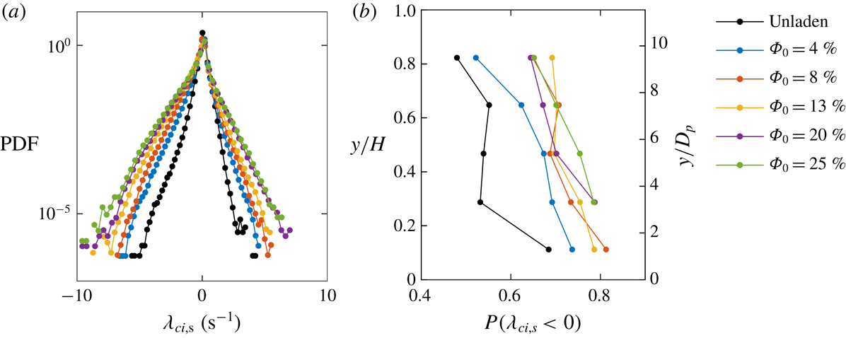
corresponds to retrograde vortices. The PDF of the signed swirling strength is plotted for all cases in figure 23(a). More extreme swirling events, both prograde and retrograde, are observed for higher
 $\unicode[STIX]{x1D6F7}_{0}$
cases. The prograde vortices are prevalent in all cases, and more so with increasing volume fraction. This may be due to the high-
 $\unicode[STIX]{x1D6F7}_{0}$
cases having significant mean shear across most of the channel height. The fraction of the prograde vortices is plotted for each case as a function of channel height in figure 23(b). (In the
 $\unicode[STIX]{x1D6F7}_{0}=20\,\%$
and 25 % cases, there are not enough fluid velocity data at the lowest location to compute converged statistics on the velocity gradients.) The frequency of prograde vortices generally decreases with height in all cases, and generally increases with
 $\unicode[STIX]{x1D6F7}_{0}$
at a given height. These trends are associated with the magnitude of the local shear: where this is relatively higher, the prograde vortices dominate. Taken together, these results suggest that the structure of the turbulence is controlled by the local mean shear, which in turn is strongly influenced by the particles’ presence.
(a) PDFs of signed swirling strength
 $\unicode[STIX]{x1D706}_{ci,s}$
for each case, where
 $\unicode[STIX]{x1D706}_{ci,s}>0$
represents retrograde motion and
 $\unicode[STIX]{x1D706}_{ci,s}<0$
represents prograde motion, and (b) the fraction of prograde events plotted for each case as a function of wall-normal distance.

The spatial structure of the turbulence is now examined by two-point statistics. The spatial correlation function of the streamwise fluctuating velocity is given by:
 $$\begin{eqnarray}R_{uu}(y_{0},x,y)=\frac{\langle u^{\prime }(x_{0}+x,y_{0}+y)u^{\prime }(x_{0},y_{0})\rangle }{\langle u^{\prime }(x_{0},y_{0})^{2}\rangle },\end{eqnarray}$$
which is independent of the horizontal coordinate of the reference point
 $x_{0}$
as the flow is developed in the streamwise direction. Figure 24 shows plots for the reference location at four different wall-normal distances
 $y_{0}$
, for all considered volume fractions. The contours are cut off at an arbitrary level of 0.7 to show the relative spatial extent of the correlations. In general, the correlation length is drastically reduced. This is a consequence of the confinement of the turbulence scales by the particles: large eddies in the fluid are either destroyed by the particles or spatially confined in the interparticle gaps. The exception is represented by the
 $\unicode[STIX]{x1D6F7}_{0}=4\,\%$
case for which, above the near-wall particle layer, the low concentration allows larger correlation lengths. Observations of the flow being much less organized in large coherent structures at increasing volume fractions were made also by Loisel et al. (Reference Loisel, Abbas, Masbernat and Climent2013) and Picano et al. (Reference Picano, Breugem and Brandt2015) for transitional and turbulent regimes, respectively. Overall, the correlation length scales decrease with
 $\unicode[STIX]{x1D6F7}_{0}$
even though the turbulent fluctuations increase, in contrast with the familiar trend in single-phase flows. This suggests that the particles act to transfer energy from large to small scales, as also demonstrated below.
Spatial correlations of the streamwise fluctuating velocity plotted at four wall-normal distances for each case. Contours are cut off at a level of 0.7 in all plots.

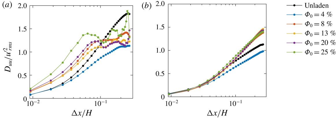
We consider the second-order velocity structure functions at a near-wall location (
 $y_{0}/H=0.1$
) and a location away from the wall (
 $y_{0}/H=0.7$
), see figure 25. The normalized second-order velocity structure function is given by:
 $$\begin{eqnarray}D_{uu}(y_{0},x)=\frac{\langle [u^{\prime }(x_{0}+x,y_{0})-u^{\prime }(x_{0},y_{0})]^{2}\rangle }{\langle u^{\prime }(x_{0},y_{0})^{2}\rangle },\end{eqnarray}$$
where only streamwise separations are considered;
 $D_{uu}(x)$
is a measure of the proportion of the turbulent energy contained in eddies of size
 $x$
and smaller. Structure functions that increase very steeply indicate that a large proportion of the energy is contained in small eddies, whereas gradually increasing structure functions indicate that energy is distributed across a wide range of scales. The normalized structure functions approach the asymptotic value of two as the streamwise separation grows arbitrarily large, the field of view setting the upper bound on the separation for which they can be calculated. Near the wall, more energy appears to be contained in large eddies for
 $\unicode[STIX]{x1D6F7}_{0}=4\,\%$
as shown by the more gradual increase with
 $x$
, whereas for higher
 $\unicode[STIX]{x1D6F7}_{0}$
relatively more energy is found at the small scales. This supports the idea that, where the local volume fraction is high (and the interparticle spacing is small), large-scale coherent fluid motion is disrupted by the particles, and the energy is transported to smaller scales. At separations greater than
 $x/H\approx 0.06$
(or
 $x/D_{p}\approx 0.7$
) the structure functions become non-monotonic for the particle-laden cases. The peaks and troughs correspond to the (quasi-)periodic spacing of the particles: the fluid motion tends to be more strongly correlated between points separated by multiples of the mean interparticle spacing. Away from the wall, differences in local volume fraction between cases are less pronounced, and in all cases the proportion of energy contained in the large scales is higher compared to the near-wall location. The comparison with the unladen flow indicates that, even at low local concentrations, the particles contribute to transferring energy to small scales.
Normalized second-order velocity structure functions each case at (a) a near-wall location (
 $y/H=0.1$
,
 $y/D_{p}=1.2$
) and (b) a location away from the wall (
 $y/H=0.7$
,
 $y/D_{p}=8.1$
).

4 Conclusions
We experimentally investigate the fluid–particle interactions in dense suspensions of finite-size particles in a turbulent boundary layer, with global solid volume fractions ranging from 4 to 25 %. The refractive-index matching between particles and fluid allows the unobstructed imaging of both phases: the particle distribution and velocity are captured simultaneously with the fluid velocity.
The particle diameter is approximately
 $1/7$
th of the unladen boundary layer thickness. Although they are only slightly denser than the fluid, the negative buoyancy results in a strong vertical concentration gradient. Discrete particle layers form parallel to the wall, increasing in number and concentration for larger volume fractions. For the more concentrated cases, the lower layers are close to the packing limit and frequent collisions and frictional contacts are likely to ensue. As a consequence, the effective viscosity of the suspension is highly increased, and local fluid velocity and velocity gradients in the near-wall region are reduced. The dense particle layers slide over each other and lag the fluid, imposing on it a strongly sheared velocity profile over large part of the channel height. This appears as a significant (and so far, unexplored) variation on inertial shear thickening: one in which both gravity-driven concentration and particle interactions play a major role. Overall, the large particles (and the discrete layers they form) produce profound deviations from the continuum limit, i.e. their effect cannot be completely accounted for by an effective viscosity.
In the immediate vicinity of the wall, turbulent stresses are inhibited by the presence of the closely spaced particles. However, above the bottom particle layer the strong mean shear acts as a powerful production mechanism and leads to much larger turbulence levels compared to the unladen flow, peaking at wall-normal locations where the local volume fraction is negligible. This regime is associated with sweeps, ejections and swirling events of uncharacteristic intensity and frequency for those wall distances.
Analysis of the spatial structure of the fluid velocity shows that the particles strongly attenuate large-scale motions where the local volume fraction is high. In these regions the turbulent velocity is only correlated over very short distances, as the tightly spaced particles disrupt large coherent structures and redistribute the kinetic energy to smaller scales of the order of the interparticle distance. Where the particles are sparse, fluid motions are not confined by the interparticle gaps, but the particles still transfer energy to smaller scales.
Future experiments shall build upon this first study to further our understanding of what is a relatively unexplored regime. Varying key parameters, such as the flow Reynolds number and the particle size and density, can help unveil the scaling of important quantities: e.g. the vertical gradients of particle concentration and particle velocity, which in turn largely drive the fluid flow properties.
Acknowledgements
This work was partially funded by the Legislative-Citizen Commission on Minnesota Resources (LCCMR). L.J.B. was supported by the Department of Defense (DoD) through the National Defense Science and Engineering Graduate Fellowship (NDSEG) Program.