





1. Introduction
Very Long Baseline Interferometry (VLBI) establishes the International Celestial Reference Frame and contributes to the International Terrestrial Reference Frame and Earth Orientation Parameters, with calibration accuracy limiting geodetic precision through its impact on scheduling optimisation (Nothnagel et al. Reference Nothnagel, Artz, Behrend and Malkin2017). Geodetic VLBI has historically operated in a dual-band configuration at S-band (2.2–2.4 GHz) and X-band (8.2–8.9 GHz), commonly referred to as legacy S/X, which has served the geodetic community since the 1970s for group-delay estimation and ionospheric correction (Thompson et al. Reference Thompson, Moran and Swenson2017). In routine geodetic S/X processing, however, the standard pipeline (e.g. HOPS fourfit) estimates only the delay-type observables and applies phase calibration via phase-cal tones (Thompson et al. Reference Thompson, Moran and Swenson2017; Cappallo Reference Cappallo2017; MIT/Haystack 2020); it does not perform absolute amplitude (flux) calibration. Where system temperature (T sys) is recorded it serves mainly for data weighting and scheduling, and amplitude calibration from T sys and antenna gain is an additional step performed only when calibrated visibility amplitudes are required, primarily for imaging (Pérez-Díez et al. Reference Pérez-Díez, Martí-Vidal, Albentosa-Ruiz, González-García, Jaron, Savolainen, Xu and Bachiller2024). Broadband station sensitivity and source flux density are therefore not routine products of geodetic processing, and recovering them is further complicated in the broadband regime (3–14 GHz) by frequency-dependent noise-diode coupling, which leaves the injected calibration tone too strong at some frequencies and too weak at others and raises amplitude-calibration uncertainties. Additional complications include increased radio frequency interference (RFI), instrumental responses that vary across frequency bands and between stations, and spectral variations among sources. Monitoring station sensitivity through T sys, System Equivalent Flux Density (SEFD), and source correlated flux densities (hereafter, flux density) requires models that capture both frequency-dependent instrumental responses and temporal variations.
Despite this critical need, existing calibration methods face significant limitations in broadband systems. Current operational practice in geodetic VLBI often updates flux densities and SEFDs on a per-session basis, using discrepancies between observed and predicted signal-to-noise ratio (SNR) aggregated over sources. While straightforward, these averages can be biased by variable sources or sparse sampling. Lim (Reference Lim2023) proposed scan-wise updates anchored to a small set of reference sources, improving robustness but still sensitive to reference selection and to broadband frequency structure. Over extended campaigns, the chosen reference sources themselves may vary in flux density or structure, or might not be observed often enough to yield a consistent reference. For broadband observations spanning multiple frequency channels, restricting calibration to a handful of sources might fail to capture the broader, frequency-dependent instrumental behaviour.
Precise flux density and SEFD estimates enable optimised observation scheduling. When the SNR is too low, group delay precision declines (Thompson et al. Reference Thompson, Moran and Swenson2017). However, an unnecessarily high SNR wastes observation time without improving group delay precision or baseline length repeatability. Because both source flux density and receiver performance vary over time, these parameters must be continuously monitored rather than treated as one-off calibration tasks.
To address these challenges, we present a Bayesian hierarchical random-walk model that jointly estimates flux density and SEFD across sessions and frequency channels. The model captures temporal changes, frequency-dependent behaviour, and instrumental variations while providing full uncertainty quantification. The model uses single-epoch catalogue anchors per source, an X-band catalogue flux density and, where an S/X ratio is available, a spectral index to seed
 $\alpha$
1, together with scan-level SNR. Reliable T
sys measurements were unavailable for these sessions and therefore could not be used. The model jointly recovers flux density and baseline SEFD across all sessions and the fitted channels with full uncertainty, information the standard geodetic group-delay pipeline does not produce.
The model encodes time dependence via random-walk processes, captures frequency dependence through piecewise spectral indices for sources and band-wise power-law scaling for SEFD, and includes an elevation-dependent SEFD correction fitted from the scan-level data. By fitting scan-level SNR observations, the model yields full posterior distributions for flux density and SEFD, enabling comparisons with flux density catalogues and informed scheduling decisions. The hierarchical structure accommodates frequency-dependent behaviours and avoids biases inherent in relying on a limited set of reference sources.
2. The Australian VLBI (AUV) observing programme
2.1. Instrumentation and recording systems
The AuScope VLBI Array, constructed in 2011 as part of Aus-tralia’s National Collaborative Research Infrastructure Strategy (Lovell et al. Reference Lovell2013; NCRIS 2006), consists of three fast-slewing 12-metre radio telescopes located in Hobart, Tasmania (Hb), Katherine, Northern Territory (Ke), and Yarragadee, Western Australia (Yg), as shown in Figure 1. Operated by the University of Tasmania, the array is a key contributor to the International VLBI Service for Geodesy and Astrometry (IVS) (Nothnagel et al. Reference Nothnagel, Artz, Behrend and Malkin2017), providing observations to several IVS observing programmes, including the Asia–Oceania VLBI network (Kurihara et al. Reference Kurihara, Lovell, Cho, Gulyaev, Shu and Kawabata2014), the AUSTRAL programme (Plank et al. Reference Plank2017), and the Australian mixed-mode programme (McCallum et al. Reference McCallum2022). Through these contributions the array improves Southern Hemisphere coverage in the global observing network.
The AuScope VLBI Array, which consists of Hobart 12 m (Hb) in Tasmania, Katherine 12 m (Ke) in the Northern Territory, and Yarragadee 12 m (Yg) in Western Australia.

During the transition to VLBI Global Observing System (VGOS) broadband operation (nominally 3–14 GHz), the AUV programme conducted repeated single-baseline sessions between Hobart (Hb) and Katherine (Ke) to characterise performance and refine the observing pipeline. These sessions provide the temporal density and scan-level SNR observations needed for hierarchical modelling of flux density and SEFD across time and frequency, and form the basis of the dataset used here.
In 2022, the Hobart and Katherine antennas were upgraded to broadband (VGOS-type) operation, providing the receiving and recording chains for the 3–13.5 GHz observations used here. They are not yet fully VGOS-compliant (their slew rates remain below the nominal VGOS specification), but their frequency coverage and signal chains support VGOS-style broadband observing. The two stations joined IVS VGOS Operations (IVS-VO) in 2023 and 2024, respectively, after resolving phase-calibration issues.
Both stations are equipped with Quad-Ridge Flared Horn receiversFootnote a covering the 2.2–14 GHz frequency range. The signal is transmitted via fibre optic cables to the control room, where it is bandpass filtered and input into the Digital Base Band Converter 3 (DBBC3) (Tuccari et al. Reference Tuccari, Alef, Dornbusch, Wunderlich, Roy, Wagner, Haas and Johansson2018) for down-conversion and sampling. The data are recorded via a FlexBuff machine in VLBI Data Interchange Format.
The AUV programme operated in two stages, differentiated by the number of channels and recording mode. During the first stage (until session auv16), each station used three input bands into the DBBC3. Each band had eight channels with a 32 MHz bandwidth, dual linear polarisation (X and Y), and two-bit sampling, yielding a recording rate of 6 Gbps. This configuration allowed for three simultaneous 4 GHz bandwidth inputs, covering the frequency ranges of 3–7, 6–10, and 9.5–13.5 GHz. This limitation was due to the old DBBC3 firmware version at Katherine (DBBC3ke), which employed the DDC mode with v124 firmware.
In the second stage starting from session auv17, the DBBC3 at Katherine was upgraded to v125 firmware, allowing four input bands, including an additional band covering the 3–7 GHz range, for a total of 32 channels, providing enhanced spectral coverage and improved frequency span for delay estimation.
The recorded data were shipped from Ke to Hb for correlation at UTAS using DiFX (Deller et al. Reference Deller2011). Fringe fitting used the Haystack Observatory Postprocessing System (HOPS) fourfit (MIT/Haystack 2020), with manual phase calibration; a detailed description of the correlation and fringe-fitting procedures is given in Jaradat et al. (Reference Jaradat, Calvés, Edwards, Ellingsen, McCarthy and Morgan2025). Manual phase calibration (pc_mode manual) was required because phase-calibration tones saturated the low-frequency channels before hardware modifications and were too weak at the highest frequencies. Reliable system-temperature (T sys) information is not available across these sessions: it was not recorded in some and is unreliable in others, owing to the same frequency-dependent noise-diode coupling. These data therefore do not permit reliable T sys-based amplitude calibration, and the analysis uses scan-level SNR. Table 1 summarises all the AUV sessions conducted for this study. A total of 31 AUV sessions were conducted; six failed, leaving 25 successfully observed and correlated sessions for the analysis. Various frequency setups were used, as RFI was identified and the observing mode was upgraded from 24 to 32 channels.
Summary of the AUV sessions, including scan lengths, relevant comments, and corresponding session dates.

Table 1. Long description
A table with 31 rows and 4 columns. The columns are labeled Session, Scan length (s), Comments, and Date. The table lists various AUV sessions, their scan lengths in seconds, relevant comments, and corresponding session dates. Row 1: Session, auv01; Scan length (s), 60; Comments, Failed power outage; Date, 2021-09-07. Row 2: Session, auv02; Scan length (s), 60; Comments, ; Date, 2021-09-23. Row 3: Session, auv03; Scan length (s), 60; Comments, ; Date, 2021-11-11. Row 4: Session, auv04; Scan length (s), 60; Comments, New frequency setup; Date, 2021-12-16. Row 5: Session, auv05; Scan length (s), 45; Comments, Turn pcal off; Date, 2022-01-17. Row 6: Session, auv06; Scan length (s), 45; Comments, ; Date, 2022-01-26. Row 7: Session, auv07; Scan length (s), 45; Comments, Failed Ke cryo failure; Date, 2022-02-08. Row 8: Session, auv08; Scan length (s), 45; Comments, ; Date, 2022-05-03. Row 9: Session, auv09; Scan length (s), 30; Comments, ; Date, 2022-04-10. Row 10: Session, auv10; Scan length (s), 30; Comments, Failed observer error; Date, 2022-04-24. Row 11: Session, auv11; Scan length (s), 30; Comments, Failed observer error; Date, 2022-05-17. Row 12: Session, auv12; Scan length (s), 20; Comments, New frequency setup; Date, 2022-06-28. Row 13: Session, auv13; Scan length (s), 20; Comments, ; Date, 2022-07-12. Row 14: Session, auv14; Scan length (s), 20; Comments, ; Date, 2022-07-25. Row 15: Session, auv15; Scan length (s), 20; Comments, ; Date, 2022-08-10. Row 16: Session, auv16; Scan length (s), 20; Comments, ; Date, 2022-08-23. Row 17: Session, auv17; Scan length (s), 20; Comments, DBBC3ke upgrade (32 ch), new freq setup; pcal on; Date, 2022-09-11. Row 18: Session, auv18; Scan length (s), 20; Comments, ; Date, 2022-09-24. Row 19: Session, auv19; Scan length (s), 20; Comments, Failed observer error; Date, 2022-10-01. Row 20: Session, auv20; Scan length (s), 20; Comments, Failed observer error; Date, 2022-10-04. Row 21: Session, auv21; Scan length (s), 20; Comments, DBBC3hb board fault (e,f samplers); Date, 2022-11-21. Row 22: Session, auv22; Scan length (s), 20; Comments, DBBC3hb board fault (e,f samplers); Date, 2022-11-28. Row 23: Session, auv23; Scan length (s), 20; Comments, DBBC3hb board fault (e,f samplers); Date, 2023-01-15. Row 24: Session, auv24; Scan length (s), 20; Comments, DBBC3hb new connection; Date, 2023-02-22. Row 25: Session, auv25; Scan length (s), 20; Comments, ; Date, 2023-03-21. Row 26: Session, auv26; Scan length (s), 20; Comments, ; Date, 2023-04-01. Row 27: Session, auv27; Scan length (s), 20; Comments, ; Date, 2023-04-23. Row 28: Session, auv28; Scan length (s), 20; Comments, ; Date, 2023-05-07. Row 29: Session, auv29; Scan length (s), 30; Comments, Scan time increased due to sensitivity; Date, 2023-05-30. Row 30: Session, auv30; Scan length (s), 30; Comments, ; Date, 2023-08-12. Row 31: Session, auv31; Scan length (s), ; Comments, SNR based; Date, 2023-09-30.
2.2. Frequency configuration
2.2.1. Selection methodology
Selecting the frequency configuration is a key step in broadband system design, balancing multiple competing objectives. This selection is difficult due to the extensive presence of global RFI across the new frequency range, the variability of local RFI in different countries, and the vast number of possible configurations. The frequency configuration also directly affects the system’s accuracy in estimating differential Total Electron Content (dTEC), resolving time delays, and reducing ambiguities, thereby enhancing the overall precision of VLBI measurements. The spanned bandwidth improves measurement precision and SNR, as does the distribution of frequency channels within the bandwidth. To evaluate the effectiveness of frequency configurations in terms of system response and the impact of ionospheric effects on observations, the two-dimensional fringe amplitude as a function of time delay and dTEC is calculated. This begins with determining the ionospheric delay induced in the phase measurements (Cappallo Reference Cappallo2017):
 \begin{align} \Delta \phi = -8.448 \times 10^9 \times \frac {dTEC}{f} \end{align}
where
 $\Delta \phi$
represents the ionospheric phase contribution in radians, dTEC is the differential TEC in TEC units (1 TEC unit = 1016 electrons/m2) along a baseline, and f is the observing frequency in Hz. Using the calculated phase delay, a complex signal is constructed and Fourier transformed to derive the two-dimensional fringe amplitude as a function of time delay and dTEC.
The resolution of the time delay and dTEC functions is defined by the width of the main lobe and the maximum height of the side lobes in the fringe amplitude. A narrower main lobe improves resolution; lower side lobes reduce ambiguity. Given the vast number of possible frequency configurations, a heuristic algorithm was developed to determine the AUV frequency configuration by considering these performance metrics while masking local RFI. RFI was included when generating the configurations rather than added as simulated noise. Frequency ranges affected by known global and site-specific (Hb and Ke) interference were identified from spectral-occupancy measurements and excluded from the allowed channel centres. Every candidate configuration was therefore drawn from the remaining frequency ranges.
2.2.2. Convergence analysis
Here a single sample denotes one complete candidate configuration, a full set of channel centres (24 or 32, depending on the hardware mode) drawn at random from the RFI-masked band and scored on the resolution metrics. A convergence analysis tracked the metrics of the top-scoring configurations against sample size. Figure 2 shows the four metrics (main-lobe width and side-lobe height for the delay and dTEC resolution functions) for a search of up to about 4 × 10⁴ configurations on a logarithmic scale. All four improve rapidly and change little beyond roughly 104 configurations. Increasing the sample size further therefore has little effect on the selected configuration (Figure 3 and Table 2).
Convergence of the four resolution metrics (main-lobe width and side-lobe height for the delay and dTEC resolution functions) for the top-scoring configurations versus sample size on a logarithmic scale. The metrics flatten beyond roughly 104 configurations, indicating that the random search over the RFI-masked frequency space has converged.

The final AUV frequency configuration. Each vertical line represents a frequency channel, and the shaded regions indicate different frequency bands.

2.2.3. Final AUV frequency configuration
Several frequency configurations were evaluated and subsequently refined to address the impacts of RFI and system limitations. The upgrade from 24 to 32 frequency channels, achieved by adding a fourth DBBC3 input band covering 3–7 GHz (Section 2.1), extended the available frequency coverage. Both the 24-channel and 32-channel configurations were independently optimised for their respective hardware capabilities using the same selection methodology; they share common design principles but differ in specific channel assignments. Figure 3 displays the final selected AUV frequency configuration, illustrating the distribution of frequency channels across different bands. Table 2 also details the exact frequency values for each channel, organised by DBBC3 sampler input (Tuccari et al. Reference Tuccari, Alef, Dornbusch, Wunderlich, Roy, Wagner, Haas and Johansson2018) rather than by ascending frequency. The sampler input ranges overlap near 6.5 GHz, so the 6 488.4 MHz channel in Band 3 lies slightly below the 6 520.4 MHz channel in Band 2.
This configuration is compared with the IVS-VO configuration in terms of delay and dTEC resolution functions, as shown in Figure 4. The AUV configuration demonstrates reduced side lobe heights for both dTEC and time delay resolution functions. The main lobe width is also slightly improved in the AUV configuration, further enhancing the resolution. This improvement reflects the advantage of optimising a frequency configuration for a specific pair of stations with well-characterised local RFI. The heuristic selection algorithm can exploit this constrained environment to distribute channels more effectively across the 3–13.5 GHz range while masking known interference bands. The IVS-VO configuration must instead accommodate a diverse global network of stations with varying local RFI environments and hardware constraints, making it more difficult to achieve uniformly low sidelobes. Frequency selection for broadband VLBI networks remains an active area of investigation within the IVS, and the selection methodology presented here may contribute to these efforts. Recomputing the delay resolution functions of both configurations confirms this quantitatively: the peak side-lobe level of the delay resolution function falls from 90.6% of the main-lobe height for the IVS-VO configuration to 59.8% for the AUV configuration (Figure 4), with the dominant side lobe in both configurations at a delay offset of ± 0.31 ns, matching the ∼300 ps sub-ambiguities reported for VGOS-type sessions with channels grouped into a few compact bands (Niell et al. Reference Niell2018). This feature is a coupled delay and dTEC ambiguity rather than a pure frequency-comb periodicity: with the IVS-VO channels concentrated in four narrow bands, a ∼300 ps delay error is nearly degenerate with a dTEC shift of only ∼5 TEC units, so the joint delay and dTEC fit retains about 90% coherence at the wrong delay; for the more uniform AUV sampling the closest such degeneracy requires an implausible ∼26 TEC units and retains only about 60% coherence. The sub-ambiguity is therefore strongly suppressed rather than removed. In the correlated AUV sessions the recorded group-delay ambiguity spacing is the full 31.25 ns set by the 32 MHz channel grid, and the as-observed side-lobe level remains near 60% in every session. A full per-session quantification across the 25 AUV sessions is deferred to a dedicated paper on the AUV frequency configuration, now in preparation.
Final AUV frequency configuration. The table lists the 32 frequency channels distributed across the four DBBC3 sampler inputs; central frequencies are shown and all channels have a width of 32 MHz.

Table 2. Long description
A table with 32 rows and 4 columns. The columns are labeled Band 1 (MHz), Band 2 (MHz), Band 3 (MHz), and Band 4 (MHz). Each row lists the central frequencies for the 32 frequency channels distributed across the four bands. Row 1: Band 1, 3 032.40; Band 2, 4 728.40; Band 3, 6 488.40; Band 4, 10 168.40. Row 2: Band 1, 3 224.40; Band 2, 4 856.40; Band 3, 7 128.40; Band 4, 10 488.40. Row 3: Band 1, 3 256.40; Band 2, 4 888.40; Band 3, 8 056.40; Band 4, 11 768.40. Row 4: Band 1, 3 736.40; Band 2, 4 920.40; Band 3, 8 184.40; Band 4, 12 216.40. Row 5: Band 1, 3 960.40; Band 2, 5 944.40; Band 3, 8 632.40; Band 4, 12 344.40. Row 6: Band 1, 4 152.40; Band 2, 6 168.40; Band 3, 8 728.40; Band 4, 12 408.40. Row 7: Band 1, 4 216.40; Band 2, 6 328.40; Band 3, 8 760.40; Band 4, 12 600.40. Row 8: Band 1, 4 504.40; Band 2, 6 520.40; Band 3, 8 888.40; Band 4, 13 272.40.
Comparison of AUV and IVS-VO resolution functions. Left: dTEC resolution. Right: delay resolution. Blue: AUV; orange: IVS-VO.

2.3. Scheduling strategy
Beyond frequency configuration, the scheduling strategy directly affects data quality and the suitability of observations for hierarchical calibration. The AUV sessions were scheduled using VieSched++ with a fortnightly cadence and 12-h session duration, constrained by the VGOS data recording rate of 1 GB/s per station. A minimum source flux density threshold of 0.8 Jy at X-band ensured adequate SNR across the broadband frequency range. The flux density threshold and fixed scan lengths were adopted because neither the station SEFDs nor the source flux densities were well known across the 3–13.5 GHz range.
The initial scan length was set at 60 s and was gradually reduced after analysing observed sessions to ensure sufficient SNR. Reducing the scan length offered two benefits: (1) an increased number of scans, and (2) a reduction in the total recorded data volume, as stations spent more time slewing between sources rather than observing them. As shown in Figure 5, the number of scans increases as scan length decreases, while the data volume correspondingly decreases. This is advantageous, given that data volume remains a primary limitation for VGOS. For instance, a 24-h session with 15-s scan lengths generates a data volume comparable to that of a 12-h session with 60-s scan lengths. The scheduler also included calibration scans of bright sources every two hours, each with a fixed scan length of 120 s. These calibration scans were used during correlation and post-processing.
The relationship between the number of scans, slew time, and the recorded data volume for a 12-h session with an 8 Gbps recording rate on the baseline Hb–Ke. The left y-axis represents the percentage values of the bar plot. The right y-axis indicates the recorded data volume in terabytes, corresponding to the line plot. The upper x-axis shows the number of scans, while the lower x-axis indicates scan time.

The sky coverage of the AUV programme was limited because only a single baseline was used. Figure 6 shows an example sky plot for a 12-h session with a sky coverage score of 0.68. This session observed 79 radio sources across 552 scans with a scan length of 45 s. Limited sky coverage affects tropospheric modelling, as fewer regions of the sky are sampled.
Sky plot for Hb and Ke during the 12-h auv08 session. This session consisted of 552 scans and 79 radio sources.

Different scan lengths were tested to maximise the number of scans while maintaining high SNR, ranging from 60 s to 45, 30, and 20 s. In sessions auv29 and auv30, the scan time was increased to 30 s due to degraded baseline SEFD. The final session adopted SNR-based scheduling instead of fixed scan lengths. This method became feasible after a calibration session estimated the stations’ SEFDs, enabling the calculation of source flux density at each observing frequency. SNR-based scheduling aimed to achieve a total scan SNR of 50, with a minimum of 5 for each frequency channel. This high SNR target was necessary due to the large uncertainty in station SEFDs and source flux densities. The SNR target was set per channel rather than per band, as the AUV frequency channels are sparsely distributed across the 3–13.5 GHz range, unlike the compact IVS-VO frequency setup. However, the programme was halted after session auv31, leaving the SNR-based scheduling method unvalidated.
The scheduling process was continuously refined to increase the number of scans and observed sources while maintaining sufficient SNR. Figure 7 illustrates the total number of scheduled and correlated scans and sources for each correlated AUV session. Sessions auv02 and auv03 were more experimental, using a limited number of sources. From auv04 onwards, scheduling became more stable. The jump in scan numbers from auv04 to auv05 resulted from reducing the scan time from 60 to 45 s, as shown in Figure 7(a). Session auv09 was the only correlated session with a 30-s scan length before transitioning to 20 s. From auv12 to auv28, the same scan length was used; however, the increase in scan numbers starting from auv21 is attributed to reducing the source switch time from 1 800 to 900 s. The mismatch between scheduled and correlated scans was caused by observational issues, primarily related to the DBBC3 system, which occasionally required restarts during sessions, resulting in missed observations.
Comparison of scheduled and correlated scans and sources across all correlated AUV sessions.

The fortnightly cadence provides the temporal resolution necessary for the random-walk model to capture gradual flux density evolution and SEFD variations, while the range of scan lengths (20–60 s) produces the scan-level SNR observations that form the basis of the hierarchical Bayesian model.
3. Bayesian hierarchical model
Bayesian statistics assigns probability distributions directly to unknown parameters, treating probability as a degree of belief (Gelman et al. Reference Gelman, Carlin, Stern and Rubin1995). Rather than producing point estimates, Bayesian inference retains the entire posterior distribution of parameters, providing full uncertainty quantification that is valuable for precise measurements in geodesy and VLBI applications.
For this application, Bayesian analysis has three advantages: it incorporates prior knowledge from earlier observations, physical constraints, or domain expertise; it handles limited data effectively, which is relevant when observations are costly or difficult to obtain; and hierarchical models, which naturally represent complex multilevel structures, are well suited to Bayesian treatment (Gelman & Hill Reference Gelman and Hill2007).
In many Bayesian analyses, computing the posterior analytically is infeasible because the evidence term
 $p(y) = \int p(y \mid \theta )$
 $p(\theta ) \, d\theta$
requires integration over all parameter values. While conjugate priors permit closed-form solutions in simple cases, hierarchical models with non-Gaussian likelihoods and high-dimensional parameter spaces typically lack such analytical tractability. These models require numerical methods (Bernardo & Smith Reference Bernardo and Smith2009).
3.1. Sampling methods
In scenarios where analytic solutions are impractical, sampling-based methods approximate the posterior distribution by generating numerous representative samples. Rather than explicitly integrating p(y), these methods explore the posterior by drawing samples that mirror its underlying probability structure. Markov Chain Monte Carlo (MCMC) algorithms provide one popular means of sampling from complex posterior distributions, producing chains of correlated samples that converge to the target distribution (Robert & Casella Reference Robert and Casella1999). Different MCMC algorithms were tested in this study, including Metropolis–Hastings, Gibbs sampling, and the No-U-Turn Sampler (NUTS), which are among the most commonly used methods (Chib & Greenberg Reference Chib and Greenberg1995; Geman & Geman Reference Geman and Geman1984; Brooks et al. Reference Brooks, Gelman, Jones and Meng2011; Hoffman & Gelman Reference Hoffman and Gelman2014). The NUTS method was chosen here; comprehensive treatments of these samplers are given in Robert & Casella (Reference Robert and Casella1999) and Brooks et al. (Reference Brooks, Gelman, Jones and Meng2011).
MCMC methods exhibit high flexibility, accommodating complex, high-dimensional models that conventional methods cannot handle. However, proper implementation demands care to ensure convergence. Typically, the initial segment of the MCMC run, referred to as the burn-in period, is discarded to reduce sensitivity to starting values. Convergence diagnostics, such as trace plots and the Gelman–Rubin statistic, further verify whether the Markov chain has stabilised (Gelman & Rubin Reference Gelman and Rubin1992).
As an adaptive variant of Hamiltonian Monte Carlo (HMC), NUTS automates trajectory-length selection, removing the need for manual tuning (Hoffman & Gelman Reference Hoffman and Gelman2014). NUTS reduces autocorrelation in the chains and accelerates convergence by utilising gradient information, making it especially advantageous for probabilistic programming libraries such as PyMC (Salvatier et al. Reference Salvatier, Wiecki and Fonnesbeck2016).
Modern probabilistic programming libraries, including PyMC, implement these MCMC algorithms in a computationally efficient manner, enabling Bayesian inference for complex models. In this paper, we employed the PyMC library to execute sampling of the Bayesian model. The sampling procedure uses the NUTS sampler, implemented via BlackJAX (Cabezas et al. Reference Cabezas2024), a high-performance HMC library optimised for probabilistic programming. BlackJAX utilises GPU acceleration, improving computational efficiency and reducing sampling time.
The following sections present a mechanistic model of the main processes driving flux density and SEFD variations. The model explicitly characterises the physical and instrumental drivers behind the observed variability, balancing model complexity against the number of free parameters.
3.2. Data structure
The AUV observational dataset comprises 25 12-h sessions conducted between September 2021 and September 2023, covering 81 radio sources that were observed in at least five sessions each, structured into the following hierarchical levels:
-
• Sources: There are N src = 81 radio sources, indexed by i ∈ {1, …, N src}, drawn from the standard geodetic VLBI source catalogue with flux densities ranging from approximately 0.8 to 5 Jy at X-band.
-
• Sessions: Observations are grouped into N sess = 25 sessions, indexed by j ∈ {1, …, N sess}. Each session is mapped to its Modified Julian Date to establish the temporal ordering that enables the time-evolution modelling. The fortnightly to monthly cadence provides the temporal resolution necessary for random-walk evolution of source flux density and SEFD while capturing gradual instrumental drifts and source variability.
-
• Frequencies: Observations cover
 $N_\nu = 32$
frequency channels, each with a bandwidth of 32 MHz, indexed by k ∈ {1, …, N
channels} or identified by their central frequencies
$\nu_k$
. The 32 channels are distributed across the 3–13.5 GHz range in a configuration optimised to reduce delay ambiguities and improve differential TEC estimation while avoiding known RFI bands (see Section 2). For pre-auv17 sessions with 24 channels, the eight additional channels introduced by the upgrade were treated as missing data in the likelihood, with the hierarchical structure borrowing strength from observed channels and sessions. The SEFD model uses four contiguous frequency intervals chosen to follow the frequency regions covered by the DBBC3 samplers (Section 3.4.3). At the small overlap near 6.5 GHz, interval membership is set by the frequency boundaries in that section. The highest channels (above ∼12 GHz, up to the channel centred at 13.3 GHz) were excluded because their low SNR near the upper band edge makes the inferred flux densities and SEFDs unreliable; the spectra (Figures 13 and 14) therefore terminate near 12 GHz, whereas Table 2 lists the full recorded configuration.
-
• Scans: Rather than labelling an individual scan, the triple (i,j,k) labels a model cell, a (source, session, channel) combination at which the model predicts flux density, SEFD and hence SNR. A source is typically observed in several scans per session, and each scan records all channels, so the data contain multiple SNR measurements per cell; these are treated as conditionally independent draws from the scan-level Gamma likelihood (Eq. 10), with the unmodelled scatter absorbed into the scale parameter
$\sigma_{i}$
, j, k
(from a per-(source, session) parameter
$\sigma_{\text{snr}}$
, i, j
). The Hb and Ke elevation angles are retained for each scan and modulate the predicted SNR through the fitted elevation factor (Eq. 8), while remaining within-cell variation, including unresolved source-structure and instrumental effects, is represented by
$\sigma_i$
, j, k
.


The single-baseline design (Hb–Ke, baseline length approximately 3 100 km) focuses inference on baseline SEFD rather than station-separated SEFD, while enabling frequency- and elevation-dependent structure. This configuration simplifies the model but precludes certain consistency checks available in multi-baseline networks, such as closure quantities. Nevertheless, the repeated session cadence and dense frequency sampling, together with partial pooling across the source, session, and frequency hierarchy, support stable posterior estimation under the adopted model. Most parameters exhibit
 $\hat{R}$
values close to 1.0 and bulk- and tail-effective sample sizes (ESS) above 400, while the autocorrelation functions for γ in the six representative sources remain near zero over the examined lags. The posterior predictive check (Figure 8) and the credible intervals reported in Appendices A and B provide further support. Data quality filtering excluded scans below 15∘ elevation to mitigate tropospheric effects and scans with integration times shorter than 15 s to ensure adequate SNR. Correlation employed the DiFX software correlator, and fringe-fitting used HOPS fourfit (see Section 2) with manual phase calibration applied when automated calibration failed, primarily at the lowest and highest frequency channels (Deller et al. Reference Deller2011; Cappallo Reference Cappallo2017; Jaradat et al. Reference Jaradat, Calvés, Edwards, Ellingsen, McCarthy and Morgan2025).
3.3. Flux density model: Hierarchical model and random walk
The flux density model represents the reference flux density for each source alongside its temporal and spectral changes. By adopting a hierarchical scheme, the model shares information across sources, which stabilises estimates even when individual sources are sparsely sampled.
3.3.1. Reference flux density
Within the hierarchical model, each source i is assigned a reference flux density F 0, i , which reflects its intrinsic brightness as determined by previous measurements or flux catalogues. This reference flux acts as a high-level parameter in the model and establishes the baseline against which all temporal variations are evaluated. Anchoring flux variability to this reference, the model can capture time-dependent deviations relative to a stable, source-specific reference. To ensure that the reference flux remains physically valid (i.e. strictly greater than zero), we specify a truncated normal prior:
 \begin{align*} F_{0,i} \sim {\rm TruncatedNormal}\bigl (\mu _{F_{0},i},\,\sigma _{F_{0},i};\; F_{0,i} \gt 0\bigr ), \end{align*}
where μ
F
0, i
and
 $\sigma_{F_{0}}$
, i
are the mean and standard deviation of the reference flux density, respectively.
External priors (e.g. the SKED scheduling catalogue) can therefore be incorporated at the source level, improving stability and mitigating parameter degeneracy. The layered formulation improves both the identifiability of parameters and the interpretability of observed flux density variations over time. Importantly, F 0, i is not fixed to catalogue values but is an estimated parameter that the data can refine. If catalogue measurements are systematically high or low, the posterior will shift F 0, i and the session offsets γ i, j to match the observed SNR via the likelihood. Partial pooling across sessions stabilises the relative temporal evolution, while the catalogue prior retains the absolute flux-density anchor.
3.3.2. Temporal evolution via random walk
To capture gradual flux density changes over time, we employ a hierarchical Bayesian structure in which session-specific flux corrections follow a random-walk process. This construction produces smooth evolutions of flux density without abrupt or unphysical transitions. The flux density observed at session j is given by:
 \begin{align} F_{i,j} = F_{0,i}\,\exp \big(\gamma _{i,j} \big), \end{align}
where γ i, j denotes the session-specific flux adjustment relative to the source’s reference flux F 0,i . This hierarchical breakdown implements partial pooling among sessions; rather than treating each session as isolated or fixing flux density at a single value over time, the model utilises information from nearby sessions to allow measured but regulated temporal changes.
The session-wise offsets γ i, j are governed by a random walk, which incorporates temporal correlation yet remains capable of capturing authentic source variability. At a chosen anchor session j epoch, the initial flux offset follows a normal prior:
 \begin{align*} \gamma _{i,j_{{\rm epoch}}} \sim {\rm Normal} \big(\mu _{\gamma _{i,0}},\,\sigma _{\gamma ,0} \big). \end{align*}
For subsequent sessions, the offset updates stochastically based on:
 \begin{align*} \gamma _{i,j+1} \sim {\rm Normal} \big(\gamma _{i,j},\,\sigma _{\gamma _{i,j}}\,\cdot \lvert \Delta t_{j+1}\rvert \big), \end{align*}
where Δt j + 1 represents the time difference between sessions, defined by:
 \begin{align} \Delta t_{j+1} = {\rm MJD}_{j+1} - {\rm MJD}_{j}. \end{align}
Note: Depending on data coverage and priors, the session drift (γ i, j ) may progress either forwards or backwards in time.
Under the assumption that radio sources remain relatively stable over short intervals, the mean of the increment (μ γ i, j ) can be set to zero, while the standard deviation (σ γ i, j ) is adjusted to reflect plausible astrophysical variability (e.g. a twofold change in flux density over one year). The posterior inference remains adaptive: the model can widen to accommodate larger variability if suggested by the data, or narrow if the data suggest smaller variability.
3.3.3. Spectral indices and frequency-dependent flux density
Sources often display spectral variations over the observing frequency. Accordingly, we incorporate spectral indices for each source, specifying two separate indices at the anchor session:
 $\alpha$
1, i, j
epoch
for frequencies below the spectral break
 $\nu$
break and
 $\alpha$
2, i, j
epoch
for frequencies above it, thus enabling a piecewise power-law representation of the flux density’s frequency dependence. We adopt a single, globally fixed break at
 $\nu$
break = 6.52 GHz. This value is close to the geometric mean of the nominal VGOS range (3–14 GHz;
 $\sqrt {3\times 14}\approx 6.5$
GHz) and lies at the lower edge of the gap between the channels centred at 6.5204 and 7.1284 GHz (Table 2). It provides a fixed division of the sampled band for the two-segment power law and is not interpreted as a source turnover or peak. The parameters
 $\alpha$
1, i, j
and
 $\alpha$
2, i, j
are the fitted slopes below and above this division. The lower-frequency segment is sampled through approximately 6.52 GHz, while the next sampled channel at 7.1284 GHz begins the upper-frequency segment. Allowing
 $\nu$
break to vary per source is left to future work. The two spectral indices evolve through the session-dependent random walk, allowing both effective slopes to change gradually with time. The complete relationship is:
 \begin{align} F_{i,j,k} = F_{i,j}\,\begin{cases} \left (\dfrac {\nu _{k}}{\nu _{0}}\right )^{-\alpha _{1,i,j}}, & \nu _{k} \le \nu _{{\rm break}}, \\[8pt] \left (\dfrac {\nu _{k}}{\nu _{0}}\right )^{-\alpha _{2,i,j}}, & \nu _{k} \gt \nu _{{\rm break}}, \end{cases} \end{align}
where
 $\nu$
0 = 8.1844 GHz is the reference frequency. Like the temporal offset parameter, the spectral indices evolve gradually following a random walk:
 \begin{align} \alpha _{p,i,j\pm 1} \sim {\rm Normal} \big(\mu _{\alpha _{p,i,j}},\,\sigma _{\alpha _{p,i,j}}\,\cdot \lvert \Delta t_{j}\rvert \big), \quad {\rm for\ } p\in \{1,2\}. \end{align}
The mean
 $\mu _{\alpha _{p,i,j}} $
can be set to zero, while the standard deviation
 $\sigma _{\alpha _{p,i,j}}$
is adjusted to reflect plausible astrophysical variability (e.g. a spectral index change of order unity over one year, corresponding to a source whose flux density ratio across the observed band changes by a factor of approximately two).
Combining the temporal offsets (γ
i, j
) with the spectral indices (
 $\alpha$
p, i, j
) yields a coherent description of flux density behaviour across both time and frequency. Because the model is hierarchical, flux densities are not estimated in isolation for each session or frequency channel; instead, they are simultaneously constrained by prior information and can adapt as new data arrive. The model uses little external information. For each source the reference-flux prior mean μ
F
0, i
is the SKED X-band value (σ
F
0, i
≈ 10%) and the prior mean of the below-break index
 $\alpha$
1, i, j
epoch
is derived from the SKED S/X ratio at that same session, while
 $\alpha$
2 has a weakly informative prior centred at zero. These priors anchor the X-band flux density and the initial below-break slope at one session. The subsequent temporal evolution, the higher-frequency spectral behaviour, the baseline SEFD, and the posterior uncertainties are inferred from the SNR data across all sessions and fitted channels.
3.4. SEFD model
The SEFD model quantifies baseline sensitivity through a combination of base and session-specific components, alongside a frequency-dependent component.
3.4.1. Reference SEFD
Similar to the flux density model, the SEFD follows a hierarchical structure designed to ensure proper parameter estimation. At the top level, all sessions are assigned to a reference SEFD, acting as the reference value from which the session-level values deviate. Its prior distribution is specified as
 \begin{align*} {\rm SEFD}_{0} \sim {\rm Normal}\bigl (\mu _{{\rm SEFD}_0},\ \sigma _{{\rm SEFD}_0}\bigr ). \end{align*}
The mean (μ SEFD0 ) and standard deviation (σ SEFD0 ) can be chosen from a previous calibration (informative priors) if available, or simply from domain knowledge (weakly informative priors) to regularise the model, which is the case here, where μ SEFD0 is set to 5 000 Jy, and σ SEFD0 is 10%. These weakly informative priors regularise the absolute flux-density and SEFD normalisation, while the likelihood constrains the relative session- and frequency-dependent variations. The multiplicative structure (exponential transformations) ensures physically positive quantities while the priors remain flexible. The posterior-predictive checks in Section 2 assess whether the fitted model reproduces the observed SNR distribution under these constraints.
Anchoring session-level values to a common reference prevents arbitrary fluctuations and maintains physical plausibility. Since SEFD influences the inferred flux density via the SNR relationship, imposing a structured prior on SEFD0 regularises the degeneracy between SEFD and flux density estimates. By employing partial pooling, the SEFD values are guided not only by the prior but also by session-specific variability. This hierarchical design allows external calibration data or domain knowledge to be incorporated systematically. Anchoring each session’s SEFD around a reference SEFD0 likewise regularises the joint inference of flux density and SEFD, mitigating bias and reducing sensitivity to uncertainties.
3.4.2. Session-level drift
To capture station performance changes and fluctuations over time, the SEFD is permitted to vary by session while remaining anchored to a reference SEFD. This variability is encoded via a session-specific multiplicative factor, so that changes to SEFD remain realistic without abrupt or unphysical shifts. The session-based SEFD is
 \begin{align} {\rm SEFD}_{j} = {\rm SEFD}_{0}\,\exp \bigl (\gamma _{j}^{{\rm SEFD}}\bigr ), \end{align}
where γ j SEFD follows a normal distribution:
 \begin{align*} \gamma _{j}^{{\rm SEFD}} \sim {\rm Normal} \big(\mu _{\gamma ^{{\rm SEFD}}},\,\sigma _{\gamma ^{{\rm SEFD}}} \big). \end{align*}
The mean μ γ SEFD is set to zero with a standard deviation on the order of 10–20%, balancing session-level flexibility against the regularisation provided by the reference SEFD.
3.4.3. Frequency slopes
To accommodate the frequency dependence of SEFD, the measured frequency range is divided into four contiguous intervals chosen to follow the frequency regions covered by the DBBC3 samplers. At the small overlap near 6.5 GHz, the interval is assigned by the boundaries below. The band index for a frequency
 $\nu$
k
is determined as
 \begin{align*} {\rm band}(\nu _k) = \begin{cases} 0, & 3\,000 \leq \nu _k \lt 4\,500, \\ 1, & 4\,500 \leq \nu _k \lt 6\,500, \\ 2, & 6\,500 \leq \nu _k \lt 9\,500, \\ 3, & 9\,500 \leq \nu _k \leq 14\,000. \end{cases} \end{align*}
Within each band, the SEFD follows a power-law dependence on frequency governed by slope parameters
 $\beta _{j,\operatorname {band}(\nu _k)}$
, where j is the session. This treatment ensures smooth frequency scaling via a power law, while also modelling additive RFI. The power-law scaling is
 \begin{align*} \left (\frac {\nu _{k}}{\nu _0}\right )^{\beta _{j,\operatorname {band}(\nu _k)}}\!, \end{align*}
where
 $\nu$
0 is the reference frequency. The slope parameters follow a normal distribution:
 \begin{align*} \beta _{j,b} \sim {\rm Normal}\bigl (\mu _{\beta },\,\sigma _{\beta }\bigr ), \end{align*}
typically centred at zero, with a standard deviation reflecting 10–20% variations within each band.
Random fluctuations induced by RFI are modelled as an additive term:
 \begin{align*} {\rm RFI}_{j,k} \sim {\rm Normal}\bigl (\mu _{{\rm RFI}},\,\sigma _{{\rm RFI}}\bigr ), \end{align*}
where μ RFI = 0 and σ RFI is set to the expected interference levels (typically a few hundred Jy).
Hence, the overall frequency-dependent SEFD is
 \begin{align} {\rm SEFD}_{j,k} = {\rm SEFD}_{j} \,\left (\frac {\nu _{k}}{\nu _0}\right )^{\beta _{j,\operatorname {band}(\nu _k)}} \;+\; {\rm RFI}_{j,k}, \end{align}
3.4.4. Elevation effects
Reliable broadband T
sys measurements are not available across these sessions, so the receiver and atmospheric contributions to the elevation dependence cannot be separated. We therefore retain the monotonic elevation correction fitted from the scan-level data over the retained scans. It is not interpreted as a measurement of atmospheric opacity or station-specific sensitivity. Let
 ${\rm elev}\_{\rm hb}_{i,j,r}$
and
 ${\rm elev}\_{\rm ke}_{i,j,r}$
be the Hobart and Katherine elevation angles (in degrees) for scan r (Eq. 10) of source i in session j; because elevation is fixed by source position and observing time, it carries no channel index k. These angles are observed values, not estimated parameters: the factor is evaluated per scan from that scan’s elevations, while the coefficients
 $\beta$
elev, 1 and
 $\beta$
elev, 2 are shared across scans. The correction takes the exponential form:
 \begin{align} \begin{aligned} {\rm ElevationFactor}_{{i,j,r}} &= \sqrt { (1 + \exp\! (\!-\beta _{{\rm elev},1}\,{\rm elev}\_{\rm hb}_{{i,j,r}} ) )} \\ &\quad \times \sqrt { (1 + \exp \! (\!-\beta _{{\rm elev},2}\,{\rm elev}\_{\rm ke}_{{i,j,r}} ) )}. \end{aligned} \end{align}
Parameters
 $\beta$
elev, 1 (Hb) and
 $\beta$
elev, 2 (Ke) are session-independent coefficients describing the fitted elevation response assigned to each antenna. Their prior distributions are truncated normal to maintain positivity:
 \begin{align*} \beta _{{\rm elev},s} &\sim {\rm TruncNorm} \big(\mu _{\beta _{{\rm elev}}},\, \sigma _{\beta _{{\rm elev}}} \big), \\ &\quad \beta _{{\rm elev},s} \geq 0, \quad s \in \{1,2\}. \end{align*}
Incorporating this factor, the final scan-level SEFD is given by:
 \begin{align} {\rm SEFD}_{i,j,k{,r}} = {\rm SEFD}_{j,k} \times {\rm ElevationFactor}_{{i,j,r}}. \end{align}
The multiplicative factor adjusts for the residual elevation dependence. Because the data are restricted to scans above 15∘ elevation, the fitted correction applies only over the retained range, where it is small and nearly flat above ∼30∘. A physical treatment would instead model the elevation-dependent system temperature as T sys(t,el) = T rec(t) + T atm[1 − exp(−τ(t)/sin el)] + T spillover, with time-variable opacity τ(t) and airmass 1/sin (el) (Blackburn et al. Reference Blackburn2019; O’Neil Reference O’Neil, Stanimirovic, Altschuler, Goldsmith and Salter2002), and convert it to SEFD using the antenna gain. Fitting this treatment requires reliable T sys measurements and multiple baselines to separate station terms; neither is available in the present data.
3.5. Likelihood function: Connecting model to data
The likelihood links predicted and observed SNR. We assume the observed SNR for each scan, denoted as
 $\textrm{SNR}_{i,\,j,\,k,\,r}^{\textrm{obs}}$
(the index r runs over the repeated scans within a model cell), is conditionally distributed following a gamma distribution. The gamma distribution is chosen due to its suitability for strictly positive, continuous data, and its flexibility in representing varying levels of data dispersion, which is appropriate for SNR measurements. Specifically, the likelihood function for each scan is defined as:
 \begin{align} {\rm SNR}^{{\rm obs}}_{ i,j,k{,r}} \sim {\rm Gamma}\big(\kappa _{i,j,k{,r}}, \lambda _{i,j,k}\big){, \quad r = 1,\dots ,R_{i,j,k}}, \end{align}
where the shape parameter (
 $\kappa$
i, j, k, r
) and the rate parameter (λ
i, j, k
) of the gamma distribution are parameterised in terms of the model’s deterministic prediction for the modal SNR (
 $\textrm{SNR}_{i,\,j,\,k,\,r}^{\textrm{pred}}$
) and a cell-level scale parameter (σ
i, j, k
). Following standard gamma parameterisation, these parameters are defined as:
 \begin{align} \kappa _{i,j,k{,r}} &= {\rm SNR}^{{\rm pred}}_{ i,j,k{,r}} \cdot \left (\frac {1}{\sigma _{i,j,k}}\right ) + 1.0, \end{align}
 \begin{align} \lambda _{i,j,k} &= \frac {1}{\sigma _{i,j,k}}. \end{align}
Here,
 $\textrm{SNR}_{i,\,j,\,k,\,r}^{\textrm{pred}}$
is deterministically computed from the cell-level flux density model (F
i, j, k
) and the SEFD model (SEFD
i, j, k, r
), whose scan dependence enters through the elevation factor of scan r (Eq. 8); the R
i, j, k
repeated scans of a cell are treated as conditionally independent draws that share the cell-level scale. The cell-level scale parameter (
 $\sigma_i$
, j, k
) is itself hierarchically modelled. It is derived from a session- and source-specific scale parameter (
 $\sigma_{\text{snr}}$
, i, j
), which is assigned a HalfNormal prior distribution to ensure positivity and to weakly regularise its magnitude. This hierarchical treatment of
 $\sigma_i$
, j, k
allows the model to adapt to varying levels of dispersion across different sources and observing sessions, implementing a form of partial pooling for uncertainty estimation.
3.6. Summary of priors and the tuning principle
The priors keep the joint flux-density and SEFD inference well posed. Two priors set the absolute scale: the per-source reference flux F
0, i
(truncated Normal centred on the SKED X-band value, standard deviation ≈ 10%) and the reference SEFD SEFD0 (Normal, mean 5 000 Jy, standard deviation ≈ 10%). The below-break index
 $\alpha$
1 is also seeded from the SKED S/X ratio at the anchor session. These priors set the absolute flux-density and SEFD normalisation, which the SNR likelihood alone cannot determine. Once this normalisation is set, the repeated scan-level observations and hierarchical partial pooling constrain the temporal, spectral, and session-dependent variations. The remaining parameters have Normal or HalfNormal priors: the random-walk steps for γ,
 $\alpha$
1 and
 $\alpha$
2, the band-wise SEFD slopes, the session-to-session SEFD dispersion, the additive RFI term, the elevation coefficients
 $\beta$
elev, s
, and the scan-level noise scale σ
snr, i, j
. Fine tuning is controlled mainly by the random-walk step widths, the session SEFD dispersion, and the RFI scale. Wider priors allow faster changes between sessions, whereas narrower priors produce smoother changes.
4. Results and discussion
This section presents the results obtained from fitting the Bayesian hierarchical random-walk model to the AUV data. We ran inference using BlackJAX with the NUTS sampler, utilising an NVIDIA GeForce RTX 4090 GPU for a single Markov chain during testing and fine-tuning. We used an NVIDIA L40S GPU for the final runs of four independent Markov chains in parallel. Each Markov chain has an initial burn-in phase of 1 000 iterations to adapt step sizes and other sampling parameters. Subsequently, the model generated 1 000 posterior draws per chain, resulting in a total of 4 000 posterior samples. The final runs took approximately two hours to process all 25 AUV sessions, each with a 12-h duration.
4.1. Convergence diagnostics
The MCMC convergence was verified using the
 $\hat{R}$
statistic, effective sample size (ESS), and autocorrelation diagnostics across four independent chains of 1 000 draws each (4 000 total posterior samples). Most parameters exhibit
 $\hat{R}$
values close to 1.0 and bulk- and tail-ESS above the recommended minimum of 400. The autocorrelation functions for γ in the six representative sources remain near zero over the examined lags. These diagnostics confirm convergence and efficient chain mixing; full details are provided in Appendix A.
4.2. Posterior predictive check
Figure 8 illustrates the comparison of the observed data with the corresponding posterior predictive distributions. The posterior predictive draws (thin blue lines) broadly cover the observed SNR, reproducing the prominent peak at lower SNR values and the tail at higher SNR, with tight clustering indicating limited model uncertainty. The posterior predictive mean (orange dashed line) consistently traces the central trend of the observed data. Draws that deviate noticeably from the posterior mean reflect the full range of parameter uncertainty captured by the model; their spread quantifies the envelope of plausible predictions rather than indicating poor fit.
Posterior predictive SNR from all 4 000 posterior draws (blue lines; orange mean) versus observed (black).

Residuals (predicted–observed SNR) with mean near zero; SD = 1.6.

To further investigate the model’s suitability and assess the overall residual distribution, the residuals of individual data points are examined. Figure 9 shows the histogram of residuals (predicted minus observed SNR), which follows a roughly Gaussian distribution centred near zero with a standard deviation of approximately 1.6, indicating no clear overall offset in the predicted SNR.
To assess the model’s predictive accuracy, we compare the model-predicted SNR values with the observed measurements across various frequencies. Figure 10 illustrates this comparison for six of the 81 sources (0104–408, 0346–279, 0748 + 126, 1124–186, 1334–127, 2355–106) selected to span a range of flux densities, spectral behaviours, and temporal variability. Session AUV28 is shown as a representative example, with observed SNR values shown in blue and model-predicted SNR in orange. The shaded region denotes the observed data variability.
Observed (blue) and predicted (orange) SNR by frequency for six sources. Shaded region: observed-data variability.

Overall, the predictions closely track the measured trends, with the predicted SNR generally falling within the observed data variability. The model captures frequency-dependent SNR variations governed by both flux density and SEFD. A key feature in all six sources is the substantial drop in SNR around 4 GHz, which is consistent across observations. This drop is attributable to persistent RFI near 4 GHz, which elevates the system noise contribution and is captured by the model as increased SEFD at those frequencies.
Beyond regions affected by RFI, the model continues to follow the observed SNR trends across the spectrum. Certain fluctuations in the measured SNR, particularly at lower and higher frequencies, likely reflect variations in source structure or instrumental behaviour. The fitted SNR follows the main observed frequency trends.
The posterior distributions of the core model parameters were examined for the six selected sources at session AUV28. The temporal evolution parameter γ is tightly constrained, with 94% Highest Density Interval (HDI) widths of order 0.05 (e.g. [−0.34,−0.29] for source 0104–408), indicating that session-to-session flux density changes are estimated with high confidence. The spectral index parameters
 $\alpha$
1 and
 $\alpha$
2 display similarly narrow posteriors, confirming that the model resolves frequency-dependent behaviour in each source. The predicted flux density at the reference frequency inherits this precision, with narrow credible intervals across all sources. Posterior distributions and trace plots for γ,
 $\alpha$
1,
 $\alpha$
2, and predicted flux density are presented in Appendix B (Figures B1–B4).
The elevation parameters
 $\beta$
elev, 1 (Hb) and
 $\beta$
elev, 2 (Ke) characterise how SEFD varies with telescope pointing angle (Eq. 8). The posterior 94% HDI for
 $\beta$
elev, 1 is [0.230,0.278], whereas
 $\beta$
elev, 2 yields [0.188,0.204] (Figure B5 in Appendix B). Because a single baseline constrains only the product of the two station responses, we do not interpret this apparent per-station difference physically. Figure 11 illustrates the resulting SEFD–elevation relationship, computed using the estimated
 $\beta$
elev, 1 and
 $\beta$
elev, 2 values and assuming a reference SEFD of 5000 Jy.
Fitted SEFD elevation correction for Hb (blue) and Ke (orange), shown over the retained range (≥ 15∘) and normalised to 5 000 Jy at high elevation. The factor is small and nearly flat above ∼30∘.

Both fitted factors remain stable at high elevations but rise towards lower elevations. The difference between the Hb and Ke factors should not be interpreted as a measured station property, as the data are restricted to elevations above 15∘, where the correction is small, and only their combined baseline response is identifiable.
While the model includes per-station elevation terms, only the baseline SEFD is identifiable on a single baseline and is reported here. Given that the dataset was restricted to scans above 15 degrees elevation, disentangling station-level estimates is neither well constrained nor critical for this study. The baseline SEFD posterior at session AUV28 yields a 94% HDI of [5 119,5 303] Jy, a tightly constrained baseline sensitivity estimate, narrower than the reference-SEFD prior (Figure B6 in Appendix B).
4.3. Predicted flux density and SEFD
We compare the recovered flux densities with the SKED catalogue and examine the predicted baseline SEFD as an indicator of system sensitivity. The SKED X-band flux density and S/X ratio at one anchor session inform the reference-flux and
 $\alpha$
1 priors. The SKED measurements at the remaining sessions are not used in the priors or likelihood and therefore provide a separate comparison of the recovered temporal evolution. SKED provides only two discrete bands (S and X) from a simplified scheduling flux model, with no per-measurement uncertainty and no SEFD (Gipson Reference Gipson2018; Schartner et al. Reference Schartner2024), whereas the present model returns continuous flux density across the fitted channels (3–12 GHz) at every session with full uncertainty.
To investigate the consistency and variability of the predicted flux densities, Figure 12 presents time-series plots for the six selected sources, with error bars representing the 94% HDI. The plots compare the flux densities predicted by the model using AUV observational data (denoted by ‘o’ with error bars) with the SKED catalogue values (denoted by ‘x’) in both S-band (orange) and X-band (blue).
Flux density time series for six sources in S-band (orange) and X-band (blue). SKED: ‘x’; model: ‘o’ with 94% HDI.

Flux density evolution reflects both intrinsic source changes and differences between measurement configurations. The SKED catalogue utilises a global VLBI network operating over 24-h session durations, incorporating multiple baselines that enhance flux density estimates via extensive uv-plane coverage. In contrast, AUV collects data on a single north–south baseline over a 12-h session, making it more susceptible to source structure and projection effects. These mainly affect the absolute flux amplitude, but because single-baseline resolution is frequency-dependent, partially resolved structure can also influence the recovered spectral shape. The observed SNR constrains the flux-to-SEFD ratio with its spectral and temporal structure, while the absolute flux scale is anchored by the X-band catalogue prior; the focus here therefore remains on the temporal and relative spectral trends.
The largely consistent temporal behaviour observed in both the SKED and AUV datasets indicates that the model recovers the flux density changes over time driven by the parameter γ, consistent with the sources’ intrinsic variability. AUV S-band flux densities are not directly inferred but are extrapolated from the spectral index parameter
 $\alpha$
1, which spans frequencies from 3 to 6.52 GHz. Because
 $\alpha$
1 is seeded from the SKED S/X ratio at the anchor session, the static S-band agreement at that session is not an independent validation. However, the agreement at the remaining sessions supports the recovered temporal evolution and shows that the model can infer flux densities at frequencies slightly outside the measured range.
The flux-density evolution of 2355–106 provides a further comparison with SKED. As depicted in Figure 12, the predicted AUV flux densities at both S-band and X-band closely track the SKED measurements, showing that the recovered temporal and spectral trends are consistent with SKED. An important feature of 2355–106 is the inversion in the relative S-band and X-band flux densities over time. Initially, the S-band flux density surpasses that of X-band, but later the trend reverses, with X-band becoming higher. The model reproduces this crossover, capturing both the temporal (γ) and spectral (
 $\alpha$
1) variation of this source. Because the priors are anchored at a single epoch, this time-dependent reversal cannot be inherited from them and is instead recovered from the SNR data. The correspondence between the extrapolated AUV S-band flux density (derived via the spectral index) and the SKED S-band measurements supports the recovered time-dependent S/X trend.
Spectral flux density for six sources. Points from inferred
 $\alpha$
1 and
 $\alpha$
2; colour encodes session. The nominal 6.52 GHz break lies at the lower edge of the gap to the next sampled channel at 7.1284 GHz, so the change of slope becomes visible above 7 GHz; channels above 12 GHz are omitted owing to low SNR.

The consistency between these two datasets, despite their different observational setups (single-baseline AUV versus a broader network for SKED), indicates that the hierarchical structure and spectral–temporal priors produce reliable flux density estimates across varied measurement contexts.
Figure 13 displays flux density as a function of frequency for the six selected sources, utilising the inferred spectral indices (
 $\alpha$
1 and
 $\alpha$
2). Different curves correspond to different epochs, showing temporal evolution in each source’s spectral properties. The figure confirms that each source exhibits evolving spectral features over time, echoing the time-dependent flux density trends discussed earlier. In particular, source 2355–106 displays a clear shift in which lower-frequency flux densities decrease while higher-frequency flux densities increase. This pattern further illustrates the model’s recovery of both spectral and temporal changes in flux density.
The six sources in Figure 13 do not share a single spectral form. Below the break the flux density generally rises with frequency, whereas above the break the behaviour diverges, with some sources continuing to rise, others flattening, and others declining; 2355–106 also departs from the common pattern in both segments. A direct comparison with T
sys is the natural check for a band-to-band SEFD systematic, but reliable T
sys is not available for these sessions (Section 2.1), so we test the concern against the independent SKED catalogue instead. In SKED (Figure 12) five of the six sources are brighter at X-band than at S-band, and 2355–106 shows the same time-dependent S/X inversion; because SKED is measured on a separate network, the rise with frequency is present in data that cannot contain the AUV SEFD. At the sessions not used to construct the priors, the recovered flux densities track the SKED values in both bands (Figure 12): a band-to-band SEFD error would tilt the recovered S/X ratios away from SKED, which is not seen, and this comparison is the closest available substitute for the requested T
sys check. A common band-dependent SEFD offset shared by all sources cannot be excluded on a single baseline, but it cannot produce the source-to-source differences, because the band-wise SEFD response (Eq. 7), including its additive RFI term, carries only session and band indices and is therefore common to every source observed in a session; it would scale every source alike and could not make one source’s spectrum rise while another’s falls. The diversity is instead carried by the per-source spectral indices
 $\alpha$
1 and
 $\alpha$
2 (Eq. 4), whose priors permit either sign. Consistent with this, the dominant SEFD feature near 4 GHz (Figure 14) is common to all six sources yet is absent from their smooth flux-density spectra, showing that the model assigns shared instrumental structure to the SEFD rather than to the individual spectral indices.

Splitting the spectrum into two segments at the nominal break of 6.52 GHz for
 $\alpha$
1 and
 $\alpha$
2 appears effective. This segmentation is beneficial as some sources exhibited two distinct spectral behaviours across this frequency range. For most sources, the two fitted segments produce comparable flux-density values around the sampled boundary, indicating that the piecewise power-law formulation captures the broad spectral variation. The break lies at the lower edge of the gap between the channels centred at 6.5204 and 7.1284 GHz (Table 2); the visible change of slope in Figure 13 therefore appears above 7 GHz, where the upper-frequency segment is first sampled.
Beyond flux density, the model also provides estimates of SEFD, a metric for quantifying system noise and overall sensitivity in VLBI observations. Evaluating SEFD across frequencies enables an assessment of system sensitivity and aids identification of potential instrumental fluctuations that may affect the observations. Figure 14 illustrates the SEFD results, with error bars that represent the 94% HDI. The estimated SEFD supports the earlier SNR findings. Specifically, session AUV24 shows overall lower SNR compared to AUV28, despite similar scheduling. This discrepancy points to high system noise or an issue with the observation during AUV24. The present SEFD estimates reinforce that conclusion, revealing consistently higher SEFD values across the full frequency range for AUV24 and thus lower system sensitivity.
The predicted SEFD values align with the observed SNR patterns. The consistently higher SEFD values in AUV24 compared to AUV28 across all frequencies indicate reduced system sensitivity. Session AUV24 followed the DBBC3 board-fault period documented for AUV21–AUV23 and used a new Hobart connection. Its higher recovered SEFD is consistent with reduced sensitivity during this hardware-transition period. In contrast, AUV28 was conducted after these problems were resolved, reflecting normal system performance. A further feature is the prominent SEFD peak around 4 GHz, corresponding to persistent RFI that elevates system noise at those frequencies.
4.4. Limitations and future work
We now discuss limitations and directions for future work.
The analysis was limited to a single-baseline configuration, which avoids the complications of a full network but does not exploit its redundancy. On a single baseline source structure cannot be separated from calibration: with only two stations no closure quantities can be formed, and the data constrain only the correlated flux density at the instantaneous uv point, not the total source flux density. We therefore do not attempt a structure correction but state how the unresolved contribution is absorbed and place its plausible magnitude in the context of the literature. As the Earth rotates over each 12-h track the projected baseline changes, so the correlated flux density of a partially resolved source is modulated within and between sessions even without intrinsic variability, and the modulation is chromatic: the fringe spacing θ ∼ λ/B falls from ∼6.7 mas at 3 GHz to ∼1.5 mas at 13.5 GHz, so a source is progressively more resolved toward the top of the band (Xu et al. Reference Xu, Savolainen, Anderson, Kareinen, Zubko, Lunz and Schuh2022).
The plausible magnitude of this effect can be placed in context using the celestial-reference-frame literature. Xu et al. (Reference Xu, Anderson, Heinkelmann, Lunz, Schuh and Wang2019) characterise source structure for 3 417 ICRF sources through the closure-amplitude rms, and broadband analyses place the corresponding delay systematic at the ∼20 ps level (Anderson & Xu Reference Anderson and Xu2018; Xu et al. Reference Xu, Anderson, Heinkelmann, Lunz, Schuh and Wang2021a). For compact, flat-spectrum calibrators the effect is generally smaller, whereas for more extended sources the structure-induced correlated-flux variation can reach tens of percent and increase towards higher frequency. Because the model contains no explicit structure term, this variation is absorbed into the nearest free parameters: time-dependent modulation into γ
i, j
and the chromatic component into
 $\alpha$
1, i, j
and
 $\alpha$
2, i, j
. Where a source is resolved, γ and
 $\alpha$
should therefore be read as effective parameters; in particular, the 2355–106 S/X behaviour, although consistent with intrinsic spectral evolution, cannot be shown on a single baseline to be free of a chromatic-structure contribution. The per-(source, session) scale term σ
snr, i, j
absorbs the within-session variation into the posterior uncertainty, mitigating but not removing the effect. A full separation requires closure phases or closure delays from at least three stations and closure amplitudes from four stations (Xu et al. Reference Xu, Heinkelmann, Anderson, Mora-Diaz, Schuh and Wang2016); none is available from the two-station Hb–Ke observations.
Extending the Bayesian hierarchical approach to multiple baselines would tie together the calibration of all baselines and exploit network redundancy. The single baseline SEFD would be replaced by per-station SEFD nodes (
 ${\rm SEFD}_{ij}\propto \sqrt {{\rm SEFD}_i\,{\rm SEFD}_j}$
); the overlap of multiple baselines at each station would help separate the station-dependent responses, while the catalogue anchors would retain the absolute flux-density normalisation. Source structure would enter as a shared per-source brightness distribution through a per-baseline, per-channel visibility-amplitude term V(u,v,
 $\nu$
), constrained jointly with full uncertainty propagation (the Bayesian analogue of self-calibration), so that closure quantities become posterior consistency checks and structure is separated from instrumental gain and intrinsic spectrum. This builds on the demonstrated imaging of radio sources from broadband VGOS data (Xu et al. Reference Xu, Savolainen, Zubko, Poutanen, Lunz, Schuh and Wang2021b) and on visibility-level structure-mitigation efforts (Kareinen et al. Reference Kareinen, Zubko, Savolainen, Xu and Poutanen2024).
These results have practical implications for geodetic VLBI operations. Improved tracking of flux density and baseline sensitivity (SEFD) can inform and optimise scheduling strategies. By combining radio astronomy calibration with time-series analysis, the model produces calibration estimates that account for temporal and spectral covariance. The calibration products from this model (updated flux density catalogues and session-specific baseline-SEFD estimates) can be ingested by scheduling software such as VieSched++ to optimise future session designs. Applied operationally within the AuScope VLBI programme, this approach would enable continuous monitoring of source and baseline parameters, contributing to more precise geodetic results and improved utilisation of broadband VLBI systems.
5. Conclusions
We have presented a Bayesian hierarchical random-walk model that jointly estimates flux density and SEFD from scan-level SNR observations across 25 AuScope VLBI sessions (81 sources; 32 channels recorded over 3–13.5 GHz, of which those up to ∼12 GHz were fitted). The partial-pooling structure avoids biases from per-session calibration or small reference sets and provides full posterior uncertainty quantification. Predicted flux densities agreed with SKED measurements from sessions not used to construct the priors, the model recovered complex spectral evolution such as the inversion in source 2355–106, and it flagged instrumental issues and persistent RFI near 4 GHz.
The current implementation is limited to a single-baseline configuration and treats observations at the amplitude level, precluding source structure separation and network redundancy checks. Extending the approach to multi-baseline arrays with station-level SEFD modelling and full interferometric visibility treatment would address these limitations.
Beyond geodetic VLBI, large connected-element arrays such as the Square kilometre Array (SKA-Low), the Deep Synoptic Array 2000 (DSA-2000), and the Atacama Large millimetre/submillimetre Array will generate abundant calibration data requiring models that account for temporal, spectral, and instrumental variations simultaneously. The random-walk approach presented here provides a foundation for such calibration systems.
Reliable T sys measurements were unavailable for these sessions, so the model uses single-epoch catalogue anchors and scan-level SNR to recover flux-density and baseline-SEFD behaviour across all sessions and the fitted channels with full posterior uncertainty. This enables flux-density and sensitivity monitoring for AuScope sessions without reliable T sys; retrospective analysis of similar legacy broadband sessions; frequency-resolved baseline-SEFD diagnostics for instrumental and RFI problems (e.g. the AUV24 anomaly and the 4 GHz feature); and per-channel flux-density catalogues with uncertainty that could support SNR-based schedule optimisation, supplying the VGOS-frequency flux models that current approaches obtain by deterministic S/X extrapolation (Schartner et al. Reference Schartner2024). The SNR-based scheduling trialled within AUV was not tested operationally, so we do not claim an end-to-end improvement.
Acknowledgments
The authors acknowledge Dr. Jamie McCallum and Dr. Warren Hankey for their valuable assistance with observing, data transportation, and correlation. This study used data collected with the AuScope VLBI array. The telescope infrastructure was established with funds provided by AuScope and the Australian Government via the National Collaborative Research Infrastructure Strategy: auscope.org.au
Data availability statement
The observational data and model implementation code are available from the corresponding author upon reasonable request.
Funding statement
This research received no specific grant from any funding agency, commercial or not-for-profit sectors.
Competing interests
The authors declare no conflicts of interest.
Appendix A. Convergence diagnostics
Verifying that the MCMC procedure has converged is essential to drawing valid conclusions from the Bayesian model. We rely on the
 $\hat{R}$
statistic (Vehtari et al. Reference Vehtari, Gelman, Simpson, Carpenter and Bürkner2021) to compare within-chain and between-chain variance, effective sample sizes (ESS) for both bulk and tail to ensure sufficiently independent draws, and autocorrelation assessments to evaluate chain mixing.
The distribution of
 $\hat{R}$
values across all parameters quantifies the ratio of between-chain to within-chain variance, serving as a primary metric of whether the MCMC chains have converged. Values near 1.0 imply good chain mixing and consistent parameter estimates. Most parameters have
 $\hat{R}$
values close to 1.0, with only a small fraction marginally higher (approximately 1.01–1.02), which remains acceptable in most Bayesian analyses. Overall, the
 $\hat{R}$
distribution indicates good convergence; mixing issues and insufficient chain lengths are not a concern.
Figure A1 presents the distributions of the effective sample size (ESS) for both the bulk (upper panel) and tail (lower panel) of the posterior (Vehtari et al. Reference Vehtari, Gelman, Simpson, Carpenter and Bürkner2021). Four MCMC chains were executed, each consisting of 1 000 iterations, yielding a total of 4 000 raw samples. The ESS corrects for autocorrelation within the chains, allowing a more accurate reflection of truly independent samples. A dashed vertical line at 400 in each panel marks a common threshold for sufficient effective sample size (Martin Reference Martin2016).
Distributions of effective sample size (ESS) for all model parameters, computed from 4 independent MCMC chains of 1 000 draws each (4 000 total posterior samples). Top panel: bulk ESS, which measures sampling efficiency in the central region of the posterior. Bottom panel: tail ESS, which measures sampling efficiency in the tails of the posterior, important for reliable credible interval estimation (Vehtari et al. Reference Vehtari, Gelman, Simpson, Carpenter and Bürkner2021). The red dashed line at 400 marks the recommended minimum for reliable posterior inference (Martin Reference Martin2016). Most parameters exceed this threshold, with many surpassing 2 000–3 000 effective samples.

Both the bulk and tail ESS histograms show that most parameters have effective sample sizes exceeding 400, often surpassing 2 000 or even 3 000. The chains mix efficiently, with a considerable number of effectively independent draws representing both central and extreme regions of the posterior. As a result, parameter estimates derived from these samples tend to have low variance. The ESS results further reinforce that the MCMC routine has converged and it provides sufficient information for posterior inference.
Figure A2 presents the autocorrelation functions (ACFs) for six randomly selected sources (0104–408, 0346–279, 0748+126, 1124–186, 1334–127, and 2355–106). These six sources are used throughout Section 4 to evaluate the model, particularly in assessing their predicted flux densities. Rather than illustrating ACFs for each parameter, we focus on these six examples to demonstrate overall mixing across the parameter space. The ACFs plot correlation values against lag, allowing for the assessment of Markov chains to determine whether they exhibit persistent dependence between iterations.
Autocorrelation functions (ACFs) of the temporal evolution parameter γ at session AUV28 for six sources: 0104–408, 0346–279, 0748+126, 1124–186, 1334–127, and 2355–106. The ACF is plotted as a function of lag for each of the four MCMC chains. Shaded bands indicate the approximate 95% confidence intervals. Near-zero autocorrelation at all lags indicates that consecutive MCMC draws are effectively independent, confirming efficient chain mixing and supporting the high ESS values reported in Figure A1.

Across all six sources, the autocorrelation functions remain near zero throughout the examined lags, indicating minimal dependence between consecutive draws. No consistent positive or negative patterns appear at higher lags, demonstrating effective chain mixing for these flux densities. In general, low autocorrelation is closely linked to higher ESS values, as fewer draws are ‘lost’ to strong correlations. These ACF plots confirm that the MCMC sampling produces well-mixed chains.
These metrics confirm that the Markov chains have converged properly, with minimal autocorrelation and abundant independent draws, so that posterior estimates remain stable.
Appendix B. Posterior distributions and trace plots
This appendix presents the posterior distributions and trace plots for the core model parameters at session AUV28. These diagnostics confirm that the chains are well mixed and that the posterior estimates reported in Section 4 are reliable.
B.1. Temporal evolution (γ)
The posterior distributions of γ, which governs the temporal evolution of the sources’ flux density, are presented in Figure B1 for six selected sources. Each line represents a different chain. These distributions exhibit a prominent peak and a relatively narrow credible interval, indicating that γ is estimated with high confidence. The 94% HDI (e.g. [−0.34,−0.29] for source 0104–408) reveals a narrow spread in estimates, and most of the posterior mass remains clustered in a tight interval. The trace plots reveal the chain’s progression across iterations. The parameter settles around a stable mean without strong trends or elevated autocorrelation, suggesting efficient chain mixing and good convergence. Examining all sources reveals a similar sampling pattern, confirming that the inferred parameters are stable and well-constrained.
Posterior density (left) and trace plot (right) for the temporal evolution parameter γ at session AUV28. The parameter γ governs session-to-session flux density changes relative to each source’s reference flux density (Eq. 2). Sources shown: 0104–408, 0346–279, 0748+126, 1124–186, 1334–127, and 2355–106. Shaded regions indicate the 94% Highest Density Interval (HDI). Each coloured line represents one of four independent MCMC chains (4 × 1 000 draws).

B.2. Spectral indices (
$\alpha_1$
,
$\alpha_2$
)


The spectral index
 $\alpha$
1 governs the variation of flux density with frequency below the break point. For the six selected sources,
 $\alpha$
1 exhibits similarly narrow and sharply defined posterior distributions (Figure B2), suggesting stable and precise inferences for each dataset. The trace plots reveal no noticeable trends or long-term drifts, ensuring efficient chain mixing and convergence. Consistent with
 $\alpha$
1, the parameter
 $\alpha$
2 demonstrates stable, well-converged traces across all six sources (Figure B3). Its posterior distributions are similarly peaked, indicating that
 $\alpha$
2 is tightly constrained.
Posterior density (left) and trace plot (right) for the spectral index
 $\alpha$
1 at session AUV28. The parameter
 $\alpha$
1 governs the power-law frequency dependence of flux density below the break frequency
 $\nu$
break = 6.52 GHz (Eq. 4). Sources shown: 0104–408, 0346–279, 0748+126, 1124–186, 1334–127, and 2355–106. Shaded regions indicate the 94% HDI. Each coloured line represents one of four independent MCMC chains (4 × 1 000 draws).

Posterior density (left) and trace plot (right) for the spectral index
 $\alpha$
2 at session AUV28. The parameter
 $\alpha$
2 governs the power-law frequency dependence of flux density above the break frequency
 $\nu$
break = 6.52 GHz (Eq. 4). Sources shown: 0104–408, 0346–279, 0748+126, 1124–186, 1334–127, and 2355–106. Shaded regions indicate the 94% HDI. Each coloured line represents one of four independent MCMC chains (4 × 1 000 draws).

B.3. Predicted flux density
The predicted flux density shows how parameter estimates translate into observable quantities. Figure B4 shows the trace plots for the predicted flux density at the reference frequency, revealing no obvious trends or extreme fluctuations and confirming the stability of the sampler. The posterior distributions are narrow, implying that the available data and model constraints yield a precise flux density estimate.
Posterior density (left) and trace plot (right) for the predicted flux density F
ref at the reference frequency
 $\nu$
0 = 8.1844 GHz for session AUV28. At the reference frequency, this quantity combines the reference flux density and the temporal evolution parameter γ. Sources shown: 0104–408, 0346–279, 0748+126, 1124–186, 1334–127, and 2355–106. Shaded regions indicate the 94% HDI. Each coloured line represents one of four independent MCMC chains (4 × 1 000 draws).

B.4. Elevation dependence (
$\beta_{\mathrm{elev},\,1}$
,
$\beta_{\mathrm{elev},\,2}$
)


In addition to the source-specific parameters, the elevation parameters
 $\beta$
elev, 1 (Hb) and
 $\beta$
elev, 2 (Ke) are examined. These parameters characterise how the SEFD varies with antenna elevation.
Both the posterior distribution and trace plots for
 $\beta$
elev, 1 (Hb) and
 $\beta$
elev, 2 (Ke) are presented in Figure B5. The posterior distributions illustrate the most probable values along with their 94% HDI, while the trace plots reveal the evolution of the parameter throughout the MCMC sampling process. Each posterior density plot includes multiple curves corresponding to different MCMC chains, enabling a visual inspection of chain mixing and convergence.
Posterior density (left) and trace plot (right) for the elevation dependence parameters
 $\beta$
elev, 1 (Hobart, top) and
 $\beta$
elev, 2 (Katherine, bottom). These session-independent parameters control how the fitted elevation factor raises the SEFD at lower elevation angles (Eq. 8). The 94% HDI is [0.230,0.278] for Hb and [0.188,0.204] for Ke. Shaded regions indicate the 94% HDI. Each coloured line represents one of four independent MCMC chains (4 × 1 000 draws).

The posterior distributions of
 $\beta$
elev, 1 and
 $\beta$
elev, 2 display well-defined peaks and well-mixed, convergent chains. On a single baseline, however, these coefficients are only jointly constrained through the product of the two station responses, so we do not interpret the individual per-station values physically. All chains converge to nearly identical distributions, which confirms complete posterior exploration. The trace plots reinforce this conclusion, revealing well-mixed chains with no evidence of drifting or excessive autocorrelation.
B.5. Baseline SEFD
The baseline SEFD posterior distribution at session AUV28 at the reference frequency is presented alongside the corresponding trace plot in Figure B6. The posterior distribution reveals the most probable SEFD values, while the trace plot serves to verify proper chain mixing and convergence.
Posterior density (left) and trace plot (right) for the baseline SEFD at the reference frequency
 $\nu$
0 = 8.1844 GHz for session AUV28. The baseline SEFD quantifies the combined system sensitivity of the Hobart–Katherine baseline (Eq. 6). The 94% HDI is [5 119,5 303] Jy. Shaded regions indicate the 94% HDI. Each coloured line represents one of four independent MCMC chains (4 × 1 000 draws).

The posterior distribution of SEFD is sharply peaked, with a 94% HDI of [5 119,5 303] Jy, indicating high confidence in the inferred value. The narrowness of this interval reflects the precision achievable under the imposed constraints. The trace plot confirms that the chains are well mixed, exhibiting neither significant drifts nor problematic autocorrelation, which validates the reliability of the posterior inference.

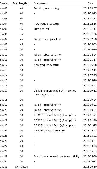
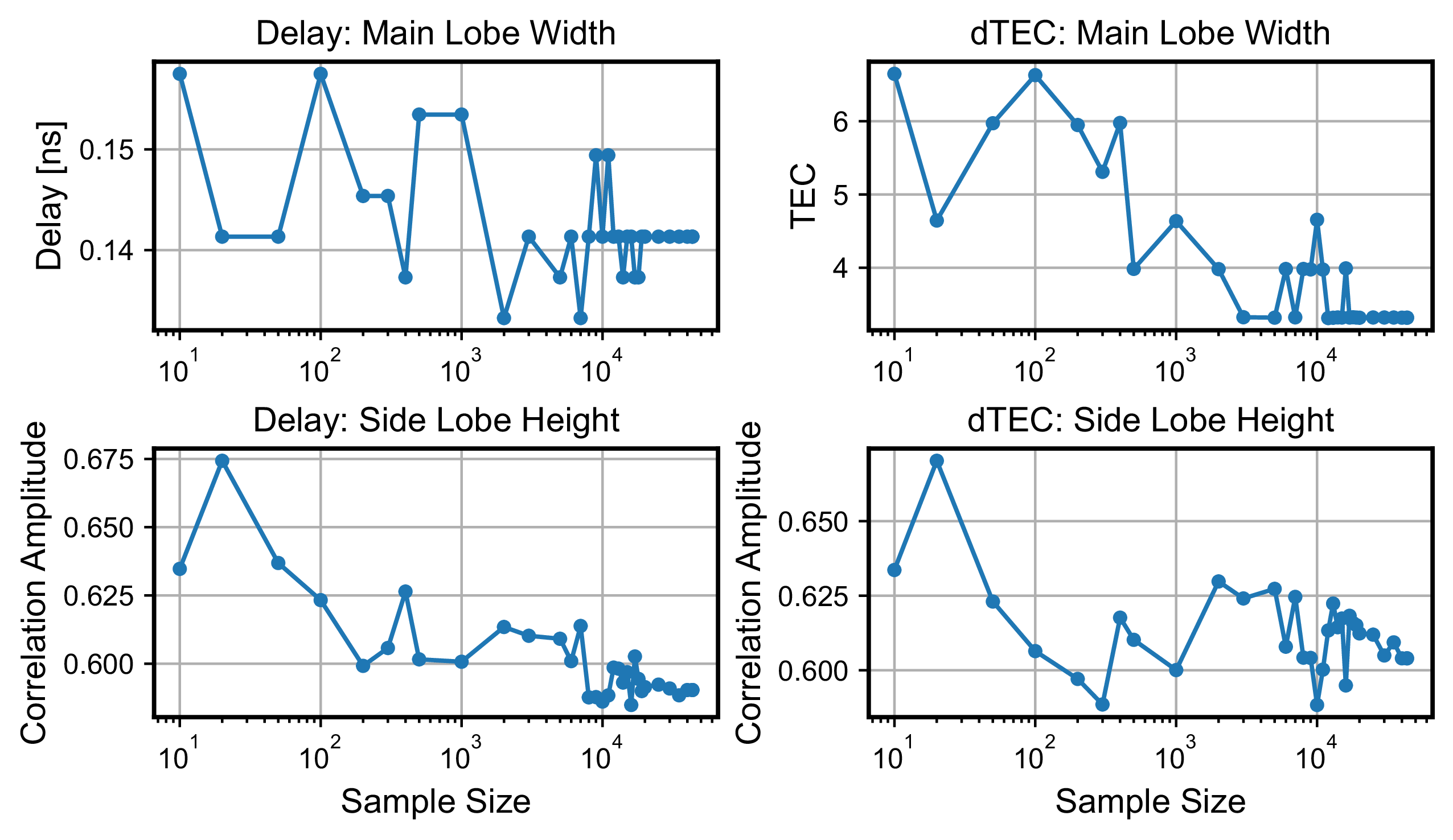
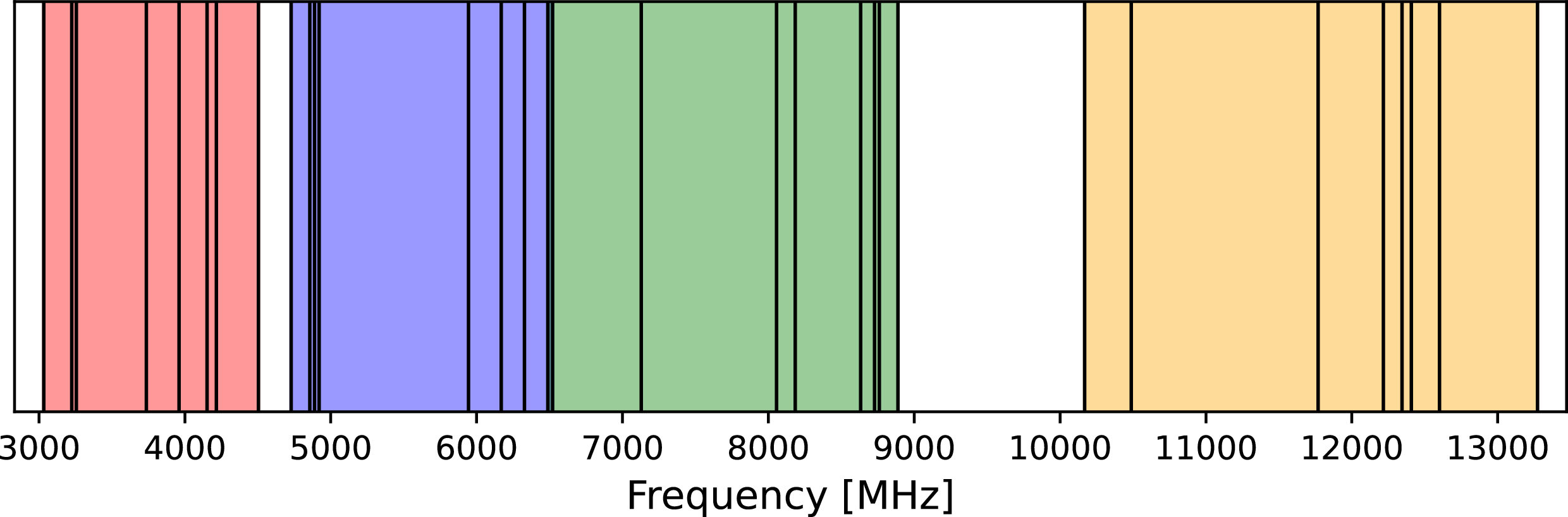
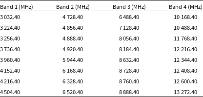
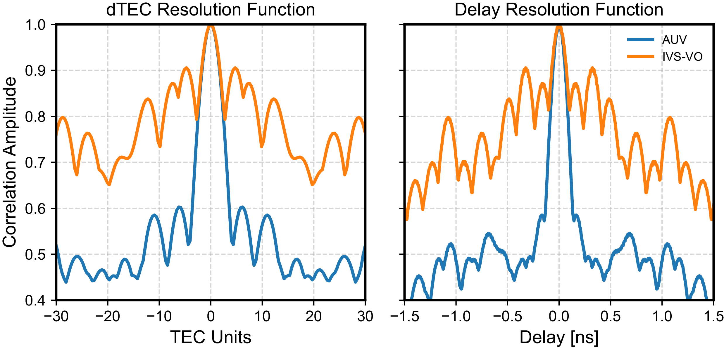
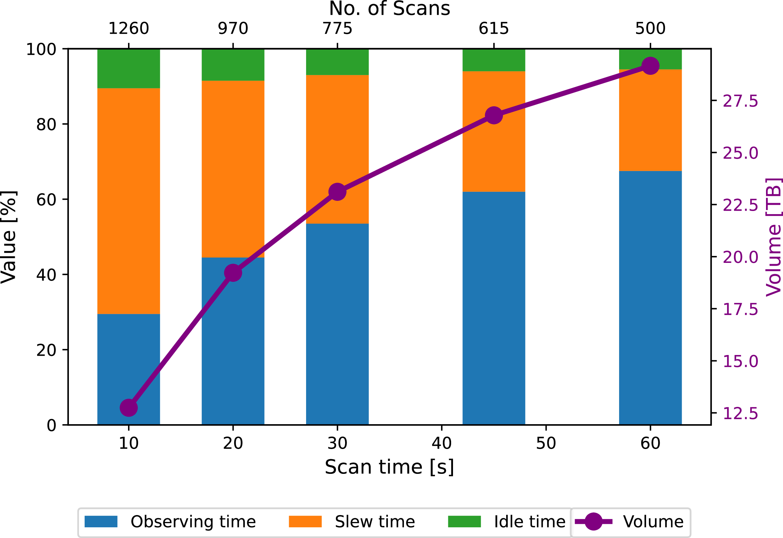


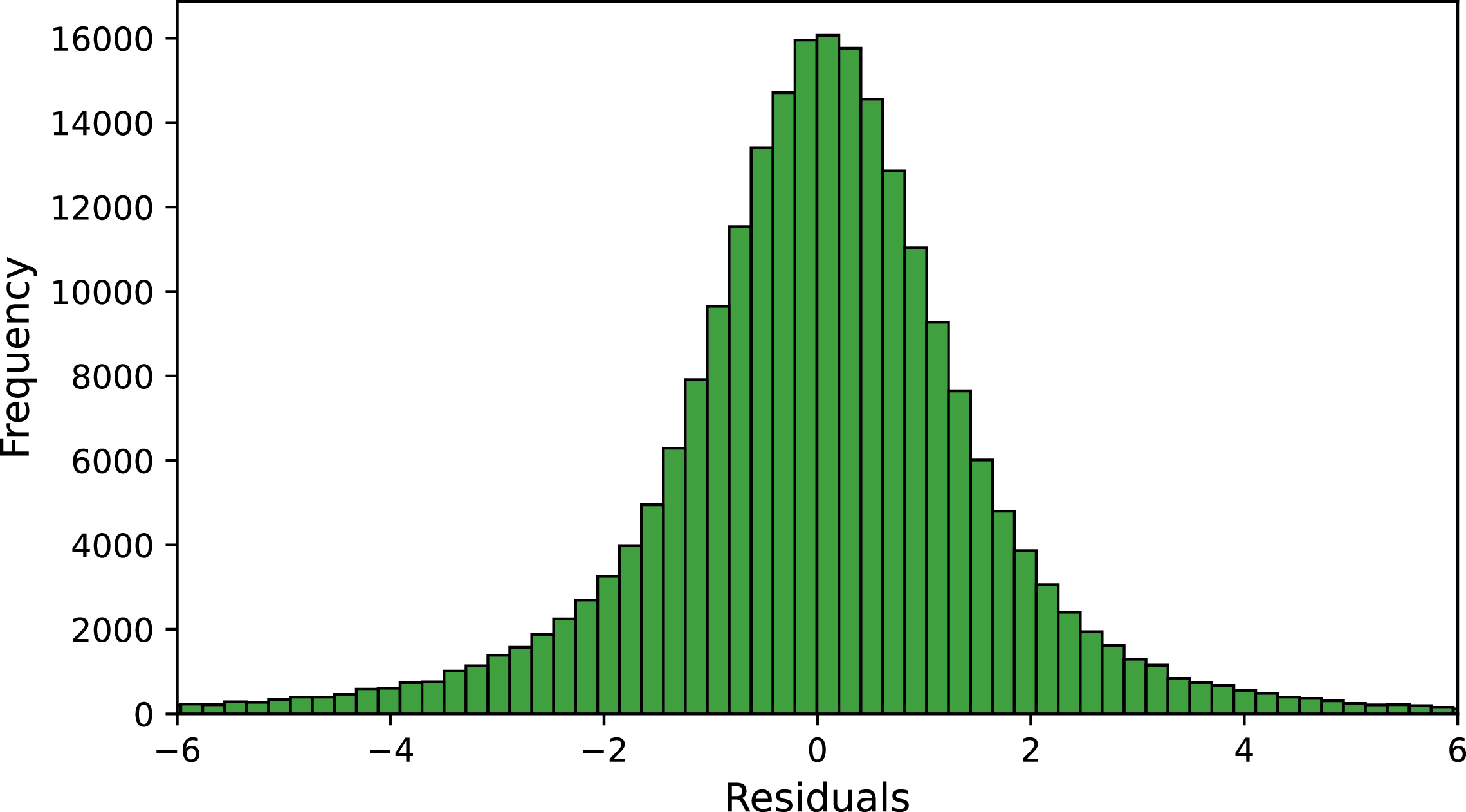

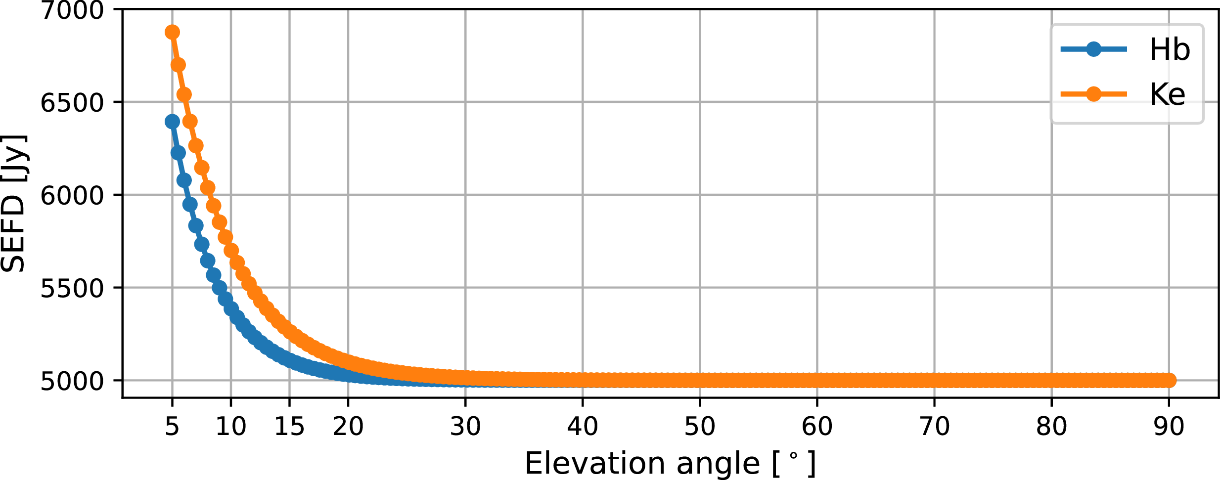


 α
 α
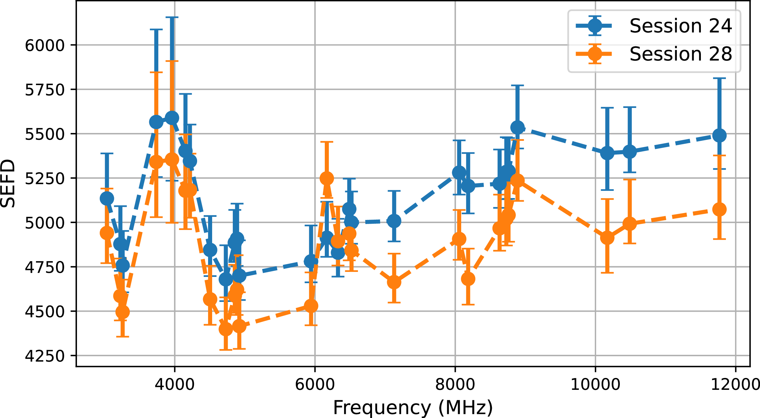
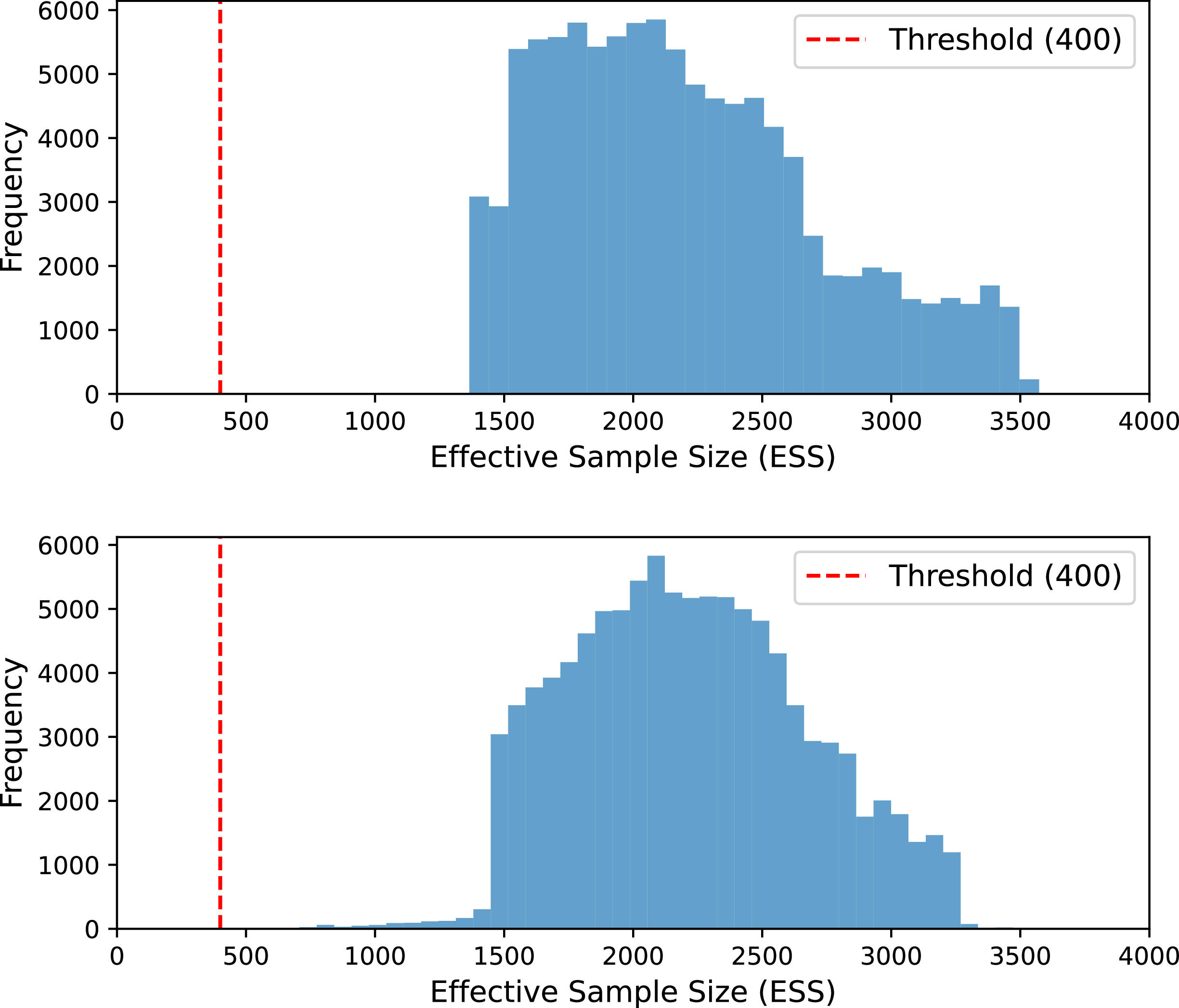
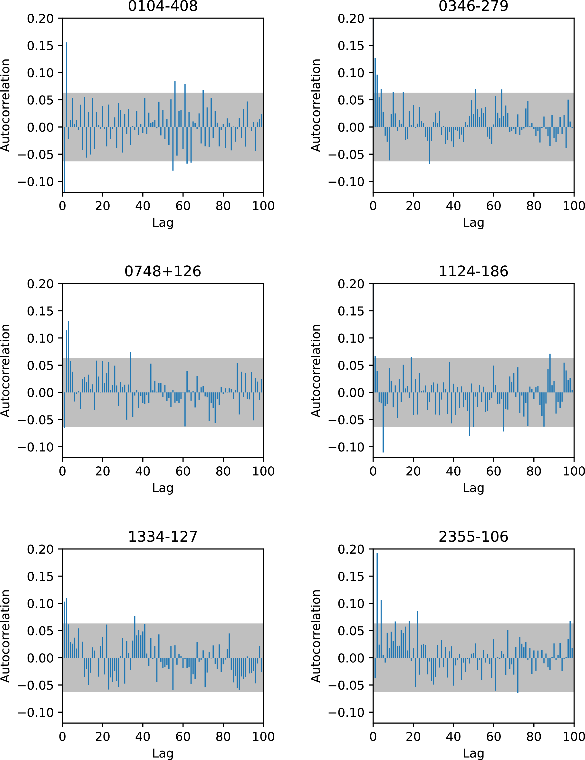


 α
 α
 ν

 α
 α
 ν

 ν

 β
 β

 ν

 Open access

