1 Introduction
In extensional flows of polymeric liquids, strong elastic stresses may arise due to the stretching of polymer molecules (Petrie Reference Petrie1979; Bird et al. Reference Bird, Armstrong, Hassager and Curtiss1987). These stresses can significantly impact the flow of a Newtonian solvent after adding a small amount of high molecular weight polymer molecules. Polymer additives are for example used to reduce the drag in turbulent pipe flows (Virk Reference Virk1975), to increase the flow rates of hose streams in firefighting (Chen et al. Reference Chen, Morales, Chen, Donatelli, Bannister and Cummings1998) and to suppress the splashing of droplets impacting on rough solid surfaces in pesticide spraying, spray coating and inkjet printing (Crooks & Boger Reference Crooks and Boger2000).
The influence of elasticity has also been investigated in industrial processes involving free-surface extensional flows such as fibre spinning (Papanastasiou et al. Reference Papanastasiou, Macosko, Scriven and Chen1987) and film casting (Alaie & Papanastasiou Reference Alaie and Papanastasiou1991; Satoh, Tomiyama & Kajiwara Reference Satoh, Tomiyama and Kajiwara2001). These techniques aim at producing plastic tubes or sheets respectively. In film casting, a polymer melt is extruded through a slot die and the resulting liquid sheet is cooled before reaching a rotating drum where it is collected. Alaie & Papanastasiou (Reference Alaie and Papanastasiou1991) report that viscoelastic films thin more rapidly at the slot exit than Newtonian films with the same viscosity. The liquids involved are generally so viscous that gravity and inertia are negligible, i.e. the force exerted by the rotating drum, which stretches the liquid in the flow direction, dominates the process.
Curtain coating is a similar process which aims at depositing a material layer of uniform thickness on a solid surface. It has been intensively investigated on geometries and situations of increasing complexity (Miyamoto & Katagiri Reference Miyamoto and Katagiri1997). A simple technique consists in pumping the desired liquid at constant flow rate from a reservoir to a precision head drilled with a long thin slot along its lower face. The sheet – or curtain – of coating liquid falls vertically from the slot before impacting a solid substrate moving horizontally underneath at constant speed. Contrary to film casting, the sheet dynamics is generally dominated by gravity since the liquids involved in curtain coating are much less viscous.
To date, although the structure of the flow is well understood in film casting, i.e. for viscoelastic sheets in the absence of gravity and inertia, very few authors have addressed the issue of the possible influence of viscoelasticity in the context of curtain coating. The existing works mostly focus on the stability of the sheet. For example, Gugler, Beer & Mauron (Reference Gugler, Beer and Mauron2010) and Becerra & Carvalho (Reference Becerra and Carvalho2011) showed that increasing the apparent extensional viscosity of the liquid reduces the minimum flow rate required to maintain a stable curtain. Karim et al. (Reference Karim, Suszynski, Griffith, Pujari, Francis and Carvalho2018b
) reported that the curtain flow of low viscosity polymer solutions with millisecond-scale extensional relaxation times was well captured by a free fall, i.e.
 $U=(U_{0}^{2}+2gz)^{1/2}$
where
 $U$
is the mean vertical velocity of the liquid,
 $U_{0}$
is the initial velocity at the slot exit,
 $z$
is the distance from the slot exit and
 $g$
is the gravitational acceleration. However, to the best of our knowledge, no similar measurements were performed on solutions with larger relaxation times. Consequently, the influence of viscoelasticity on the curtain flow remains an open question.
The structure of the flow is well documented for Newtonian liquid curtains. Investigations started in the 1960s when Taylor proposed, in the appendix of Brown (Reference Brown1961), the following one-dimensional force balance equation
 $$\begin{eqnarray}U\frac{\text{d}U}{\text{d}z}=g+\frac{4\unicode[STIX]{x1D702}U}{\unicode[STIX]{x1D70C}}\frac{\text{d}}{\text{d}z}\left(\frac{1}{U}\frac{\text{d}U}{\text{d}z}\right),\end{eqnarray}$$
where
 $\unicode[STIX]{x1D70C}$
and
 $\unicode[STIX]{x1D702}$
are respectively the liquid density and dynamic viscosity. This equation was found to capture the experimental results by Brown (Reference Brown1961) and an analytical solution was found by Clarke (Reference Clarke1966, Reference Clarke1968). The main result is that viscous dissipation only affects the liquid velocity within a distance from the slot exit which scales as
 $$\begin{eqnarray}z_{v}=((4\unicode[STIX]{x1D702}/\unicode[STIX]{x1D70C})^{2}/g)^{1/3},\end{eqnarray}$$
(‘
 $v$
’ for ‘viscous’) with a prefactor which is a decreasing function of the initial velocity
 $U_{0}$
and which is of order
 $7$
for small initial velocities
 $U_{0}\ll \sqrt{gz_{v}}$
. The liquid initially falls with sub-gravitational accelerations for
 $z\ll z_{v}$
, i.e.
 $U\text{d}U/\text{d}z<g$
, and finally reaches an asymptotic free-fall regime of constant acceleration
 $g$
for
 $z\gg z_{v}$
. However, the length of the sub-gravitational regime is generally much smaller than the length
 $L_{c}$
of the curtain, i.e.
 $z_{v}\ll L_{c}$
. Typical orders of magnitude are
 $z_{v}=0.01~\text{cm}$
for water of viscosity
 $\unicode[STIX]{x1D702}=10^{-3}~\text{Pa}~\text{s}$
and
 $z_{v}=1~\text{cm}$
for pure glycerin of viscosity
 $\unicode[STIX]{x1D702}=1~\text{Pa}~\text{s}$
, while a typical curtain falls over a distance
 $L_{c}=10~\text{cm}$
. Hence, for low viscosity Newtonian liquids, the flow is often approximated by a free fall.
To date, the length of the sub-gravitational regime remains unknown in the case of viscoelastic curtains. This gap in the literature might lead some authors to assume, incorrectly, that the flow of viscoelastic curtains or jets can be approximated by a free fall based on the small value of the viscous length
 $z_{v}$
. In this paper, we aim at filling this gap by investigating experimentally the influence of viscoelasticity on the curtain flow. Low viscosity polymer solutions are extruded from a slot die at constant flow rate and the liquid falls onto a motionless solid surface. We show that the liquid falls with sub-gravitational accelerations up to a distance from the slot which scales as
 $z_{e}=g\unicode[STIX]{x1D70F}_{fil}^{2}$
(‘
 $e$
’ for ‘elastic’) which can be much larger than
 $z_{v}$
, where
 $\unicode[STIX]{x1D70F}_{fil}$
is the polymer extensional relaxation time. By analogy with Newtonian curtains, we show that the velocity field
 $U(z)$
rescales on a master curve. Besides, the flow is shown to be only weakly affected by the history of polymer deformations upstream of the curtain. We also confirm that adding polymer stabilises the curtain by reducing the minimum flow rate required to maintain a continuous sheet.
This manuscript is organised as follows. Sections 2 and 3 describe respectively the experimental set-up and the rheology of the polymer solutions. The experimental results are given in § 4, followed by a theoretical treatment in § 5. The role of pre-shear upstream of the curtain is investigated in § 6 and the role of viscoelasticity in curtain stability is investigated in § 7.
2 Materials and methods
2.1 Polymers and preparation of the solutions
Experiments are performed with aqueous solutions of two high molecular weight polymers with different rheological behaviours. For each curtain experiment,
 $M=5~\text{kg}$
of solution is required.
We use solutions of polyethylene oxide (PEO) of molecular weight
 $M_{w}=8\times 10^{6}~\text{g}~\text{mol}^{-1}$
. The solvent is a Newtonian aqueous solution of polyethylene glycol (PEG) of low molecular weight
 $M_{w}=8000~\text{g}~\text{mol}^{-1}$
which is used as a thickener (Dontula, Macosko & Scriven Reference Dontula, Macosko and Scriven1998; Becerra & Carvalho Reference Becerra and Carvalho2011; Karim et al.
Reference Karim, Suszynski, Griffith, Pujari, Francis and Carvalho2018b
). Both polymers are provided by Sigma-Aldrich (refs 372838 and P2139). In most solutions, the PEG concentration is
 $[\text{PEG}]=20$
wt% and the corresponding solvent viscosity is
 $\unicode[STIX]{x1D702}_{s}=0.017~\text{Pa}~\text{s}$
. The PEO concentration ranges between 0 (pure solvent) and 0.4 wt%. A
 $5~\text{kg}$
solution is prepared by first adding the desired mass of PEO (20 g for a 0.4 wt% PEO concentration) to 3 kg of pure water. The granular polymer particles are slowly added into the vortex created by a mechanical stirrer which is then used for 15 h to ensure homogeneous mixing. Finally, another solution of 1 kg of PEG and 1 kg of water is prepared and the two solutions are mixed. The final solution is shaken for about 2 h before use. Following a similar protocol, other solutions are prepared with a higher PEG concentration
 $[\text{PEG}]=40$
wt%. The corresponding solvent viscosity is
 $\unicode[STIX]{x1D702}_{s}=0.14~\text{Pa}~\text{s}$
.
We also use solutions of partially hydrolysed polyacrylamide (HPAM). This polyelectrolyte is provided by SNF Floerger (ref Floset 130 VG). Molecular weight is estimated to be approximately
 $M_{w}=15{-}20\times 10^{6}~\text{g}~\text{mol}^{-1}$
and the hydrolysis degree is close to 30 %. At equilibrium in water, HPAM molecules are swollen due to repulsive electrostatic charges along the chain backbone and behave as semi-rigid rods, in contrast to PEO molecules which behave as flexible coils. HPAM rigidity can be tuned by adding salt to the solution (Cartalos & Piau Reference Cartalos and Piau1992; Kawale et al.
Reference Kawale, Marques, Zitha, Kreutzer, Rossen and Boukany2017). As salt is added, the repulsive interactions are screened and HPAM molecules become more flexible, i.e. their radius of gyration decreases (Zhang et al.
Reference Zhang, Zhou, Zhai, Liu and Gao2008; Chen et al.
Reference Chen, Yao, Liu, Luo, Zhou and Jiang2012). In order to investigate the influence of polymer conformation on the curtain flow, we use aqueous solutions of fixed polymer concentration [HPAM]
 $=$
0.1 wt% and various salt concentrations [NaCl] ranging between 0 and 10 wt%. A 5 kg solution is prepared by adding 5 g of HPAM powder to 5 kg of pure water and shaking for 15 h to ensure homogeneous mixing. The desired mass of salt is finally added and the final solution is shaken for a few minutes before use. The solvent viscosity is
 $\unicode[STIX]{x1D702}_{s}=0.001~\text{Pa}~\text{s}$
.
As will be commented in § 3.4, mechanical degradation can occur during shaking, as is expected from the use of a mechanical stirrer which is a high shear-rate mixing technique. This can result in a lower average molecular weight
 $M_{w}$
. Hence, the rheological behaviour of any new solution has to be characterised independently.
For a given solvent, density
 $\unicode[STIX]{x1D70C}$
and surface tension
 $\unicode[STIX]{x1D6FE}$
, which is measured by a pendant drop method (Daerr & Mogne Reference Daerr and Mogne2016), were found not to depend on polymer concentration. Values are
(i)
 $\unicode[STIX]{x1D70C}=1000~\text{kg}~\text{m}^{-3}$
and
$\unicode[STIX]{x1D6FE}=72~\text{mN}~\text{m}^{-1}$
for HPAM solutions.
(ii)
$\unicode[STIX]{x1D70C}=1026~\text{kg}~\text{m}^{-3}$
and
$\unicode[STIX]{x1D6FE}=62~\text{mN}~\text{m}^{-1}$
for PEO solutions with 20 wt% PEG solvent.(iii)
$\unicode[STIX]{x1D70C}=1070~\text{kg}~\text{m}^{-3}$
and
$\unicode[STIX]{x1D6FE}=53~\text{mN}~\text{m}^{-1}$
for PEO solutions with 40 wt% PEG solvent.






2.2 The hydraulic loop
Schematic of the hydraulic loop (a) and of the slot die (b).
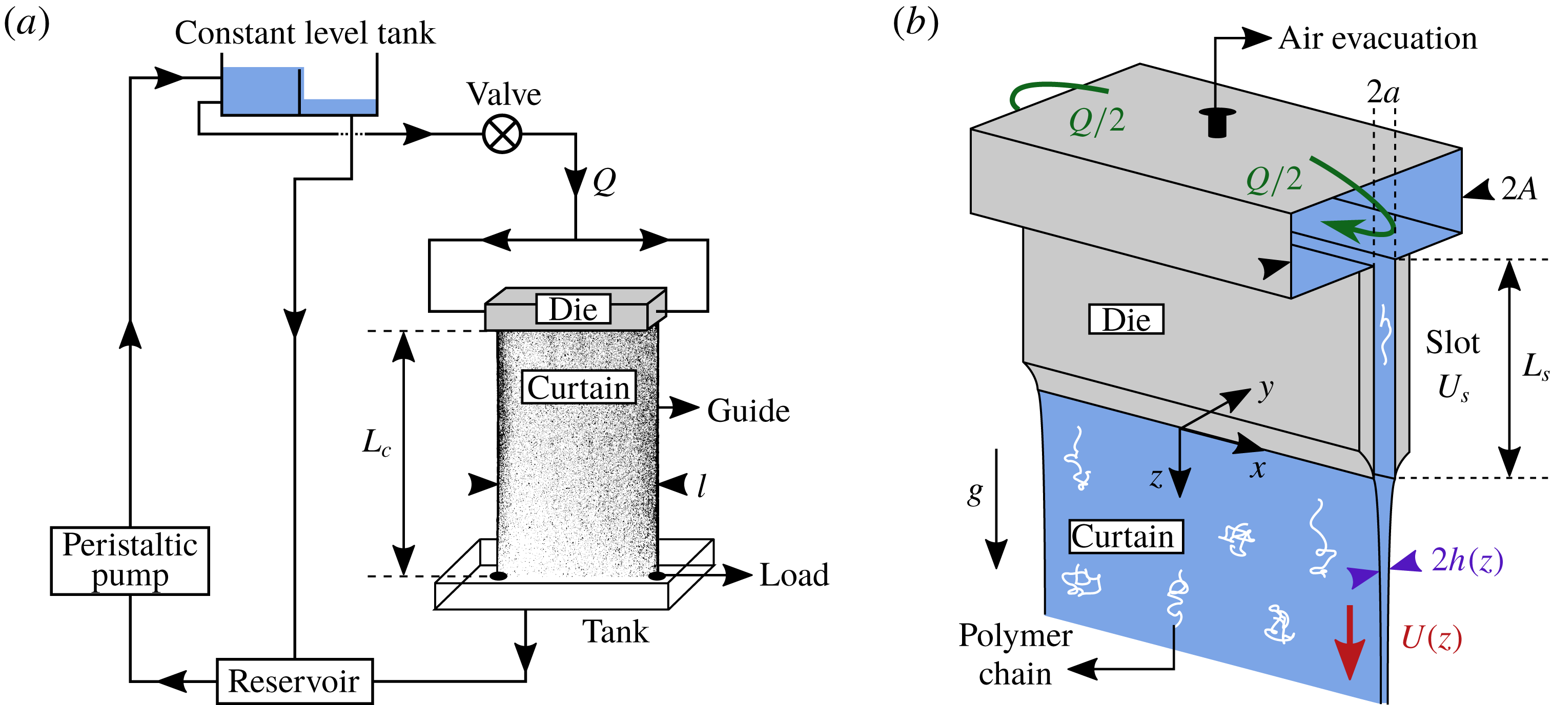
Most of the curtain experiments were conducted with the hydraulic loop sketched in figure 1(a). The polymer solution is pumped from a reservoir with a peristaltic pump up to a constant level tank, from which it flows down to a slot die (approximately 2 m below the tank) by gravity. The liquid then falls vertically from the slot down to a tank, forming a rectangular curtain of width
 $l=14.5~\text{cm}$
and length
 $L_{c}$
ranging from 15 cm up to 200 cm. To avoid sheet retraction due to surface tension, the liquid is guided between two wires (cooking strings) held vertically with loads on the tank surface. The liquid then flows back to the reservoir, thus closing the loop. The liquid mass flow rate
 $Q$
feeding the die is controlled by a valve and is measured directly by weighing;
 $Q$
is lower than the flow rate imposed by the pump, and the liquid excess flows directly from the constant level tank to the reservoir. This ensures that the liquid level is constant over time. The pulsations caused by the peristaltic pump vanish when the liquid enters the constant level tank, which ensures that the die is fed by a stationary flow. We define the linear flow rate (volumetric flow rate per unit width) as
 $q\equiv Q/\unicode[STIX]{x1D70C}l$
.
2.3 The die
In figure 1(b) we present the geometry of the die. The liquid enters on both sides of a hollow box of width
 $2A=14~\text{mm}$
and then flows through a slot of length
 $L_{s}=10~\text{cm}$
, width
 $l$
and thickness
 $2a=1~\text{mm}$
. The contraction ratio is
 $A/a=14$
. The air inside the die is evacuated using a small hole on top of the box. Once the die is full of liquid, the hole is closed. The slot consists of two flat walls which were carefully designed to ensure a constant separation distance. The wall edges are bevelled to prevent wetting of the liquid when leaving the slot. The initial curtain thickness
 $2h(z=0)$
is thus expected to be equal to
 $2a$
. Equivalently, the initial mean velocity of the curtain at the slot exit
 $U_{0}\equiv U(z=0)$
is expected to be equal to the mean velocity
 $U_{s}=q/2a$
in the slot.
2.4 Flow visualisation
We measure the velocity field of the curtain in the
 $x{-}z$
plane using the particle image velocimetry (PIV) technique. Polymer solutions are seeded with solid polyamid particles (PSP) of diameter
 $50~\unicode[STIX]{x03BC}\text{m}$
and density
 $1.03~\text{g}~\text{cm}^{-3}$
(provided by Dantec Dynamics) at a concentration of 0.04 wt% corresponding to a volume fraction of
 $4\times 10^{-4}$
. We have checked that these tracers had no influence on the rheology of the solutions. The curtain is illuminated with a white continuous light source and is filmed with a high-speed camera. Note that, due to the finite size of the PIV correlation windows, the first value
 $U_{1}=U(z_{1})$
of the velocity field is measured at a distance
 $z=z_{1}\approx 2.5~\text{mm}$
below the slot exit. We do not measure the
 $y$
dependence of the flow field with the technique described in this section.
Example of PIV measurement for a 0.2 wt% PEO solution with 20 wt% PEG solvent after 10 min in the hydraulic loop. (a) Superposition of eleven successive PIV images where some tracers are highlighted for clarity. Due to edge effects, the correlation algorithm is applied to a domain restricted to the dashed rectangle. (b) The
 $z$
-component of the velocity field, i.e.
 $U(x,z,t)$
, against the horizontal coordinate
 $x$
at different distances
 $z$
from the slot at an arbitrary time
 $t$
. The curtain length is
 $L_{c}=30~\text{cm}$
and the linear flow rate is
 $q=2.3~\text{cm}^{2}~\text{s}^{-1}$
.
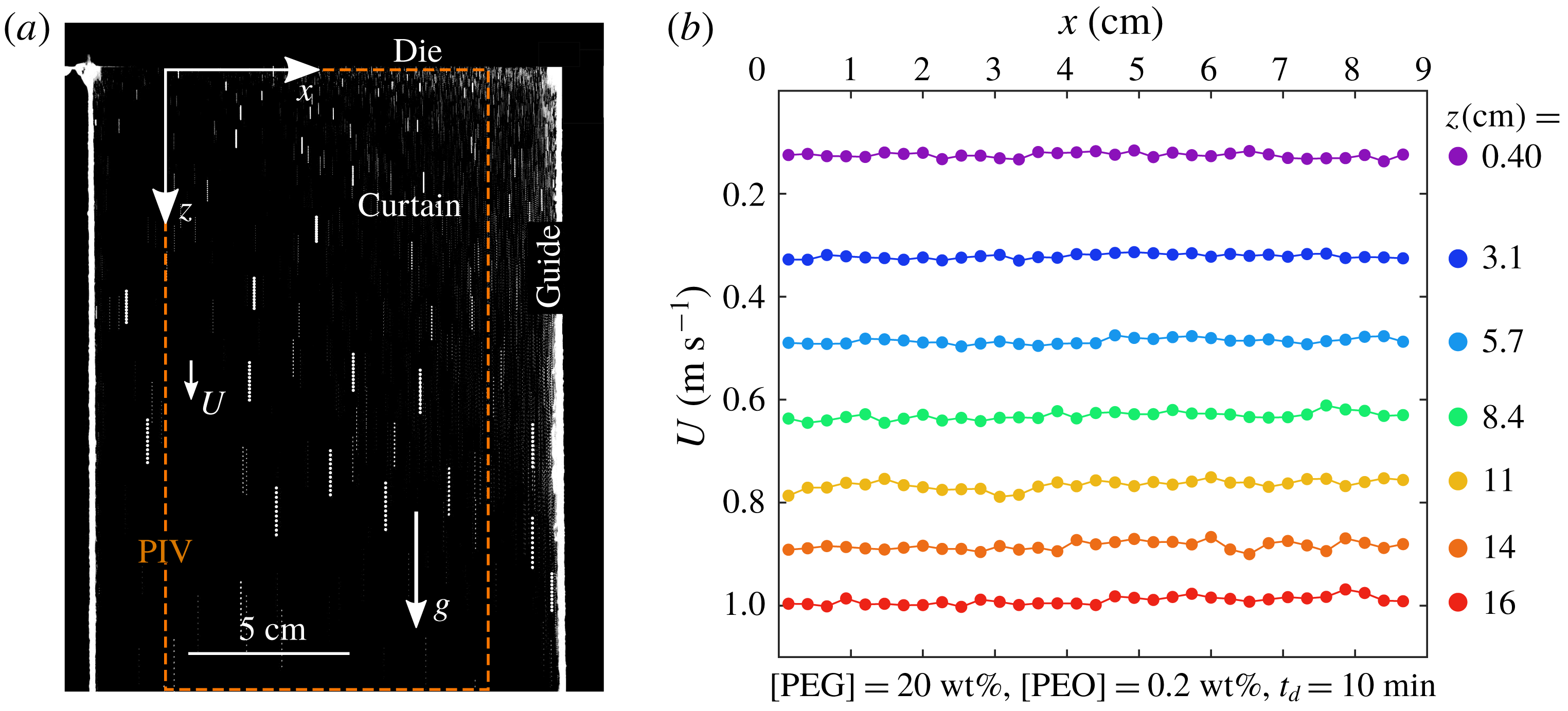
In figure 2(a), we show a superposition of eleven successive curtain images for a 0.2 wt% PEO solution with 20 wt% PEG solvent. Note that the falling velocity decreases down to 0 when approaching the vertical immobile guides (not visible in figure 2
a). This is the consequence of boundary layers developing along both guides. We measure that PEO and HPAM curtains are only affected within less than 2 cm from the guides at
 $z=20~\text{cm}$
from the slot. Therefore, the image correlation algorithm is applied to a domain restricted to the dashed rectangle in figure 2(a). As also observed by Karim et al. (Reference Karim, Suszynski, Francis and Carvalho2018a
), this effect is much more pronounced for highly viscous Newtonian liquids such as pure glycerin (
 $\unicode[STIX]{x1D702}\approx 1~\text{Pa}~\text{s}$
), for which the boundary layer reaches a size of approximately 4 cm at
 $z=20~\text{cm}$
, and honey (
 $\unicode[STIX]{x1D702}\approx 10~\text{Pa}~\text{s}$
) for which it invades the whole curtain at
 $z=10~\text{cm}$
.
Once a curtain is formed, images of the flow are recorded during 2 s. An example of velocity field obtained by processing a pair of successive images is given in figure 2(b) for a 0.2 wt% PEO solution with 20 wt% PEG solvent. We measure that the
 $x$
component of the velocity field is 0, as expected. Therefore, we plot the
 $z$
component
 $U(x,z,t)$
against
 $x$
for various distances
 $z$
from the slot at an arbitrary time
 $t$
. Since the flow is fairly independent of
 $x$
,
 $U$
is averaged along
 $x$
to give
 $\langle U\rangle _{x}$
which is a function of
 $z$
and
 $t$
. Repeating this procedure for different image pairs shows that the flow is stationary. Therefore,
 $\langle U\rangle _{x}$
is averaged over 40 image pairs, equally spaced in time, and we finally obtain
 $U(z)\equiv \langle \langle U\rangle _{x}\rangle _{t}$
. The curtain flow is stationary and translation invariant along
 $x$
for most of the data presented in this paper. However, some exceptions are observed, as will be investigated in a separate section for clarity (see § 4.2).
2.5 Experimental limitation: the accessible range of flow rates
For a given liquid, the maximum accessible flow rate
 $Q_{max}$
feeding the die (when the valve is completely open) can either be determined by the maximum flow rate achievable by the pump (for this liquid) or by the dissipation in the slot. In the latter case,
 $Q_{max}$
decreases when increasing the polymer concentration since the liquid viscosity increases. On the other hand, the die has to be fed with a minimum flow rate
 $Q_{min}$
in order to form a continuous curtain. We observe that
 $Q_{min}$
decreases with increasing the polymer concentration, as will be discussed in § 7. The resulting range of accessible flow rates
 $Q_{min}{-}Q_{max}$
goes from
 $5{-}10~\text{g}~\text{s}^{-1}$
for large polymer concentrations to
 $20{-}80~\text{g}~\text{s}^{-1}$
for low polymer concentrations. In the latter case, the convenient range is closer to
 $50{-}80~\text{g}~\text{s}^{-1}$
since many holes may puncture the curtain at low flow rates.
For these reasons, the experiments presented in this manuscript are performed with flow rates
 $Q$
ranging from
 $6~\text{g}~\text{s}^{-1}$
for large polymer concentrations to
 $60~\text{g}~\text{s}^{-1}$
for low polymer concentrations, i.e. the mean velocity
 $U_{s}=q/2a=Q/2a\unicode[STIX]{x1D70C}l$
in the slot ranges between
 $0.04~\text{m}~\text{s}^{-1}$
and
 $0.4~\text{m}~\text{s}^{-1}$
.
3 Rheology of polymer solutions
In this section, we present two distinct series of shear and extensional rheology measurements. First, in order to characterise the polymer solutions, we performed purely rheological measurements on various PEO solutions with 20 wt% PEG solvent and on 0.1% HPAM solutions with various salt concentrations at
 $T=20\,^{\circ }\text{C}$
. The PEO solutions are obtained by dilution of a 0.2 wt% stock solution (except for 0.3 and 0.4 wt% solutions which are prepared independently) while HPAM solutions were obtained by addition of different salt weight fractions to samples of a 0.1 wt% HPAM stock solution. The rheological characterisation of these solutions is presented in §§ 3.1–3.3. Then, the rheological characterisation of the specific 5 kg solution used in curtain experiments (including PEO solutions with 40 wt% PEG solvent) will be commented separately in § 3.4.
3.1 Shear rheology
For shear rheology measurements, we use a strain-controlled rheometer (ARES-G2) from TA Instruments equipped with a cone-plate geometry of radius
 $R_{1}=25~\text{mm}$
, angle
 $\unicode[STIX]{x1D703}_{1}=0.04~\text{rad}$
and truncation gap 0.055 mm. Temperature is controlled by a Peltier device. We measure the apparent shear viscosity
 $\unicode[STIX]{x1D702}=\unicode[STIX]{x1D70E}_{12}/\dot{\unicode[STIX]{x1D6FE}}$
as well as the first normal stress difference
 $N_{1}=\unicode[STIX]{x1D70E}_{11}-\unicode[STIX]{x1D70E}_{22}$
, where
 $\dot{\unicode[STIX]{x1D6FE}}$
is the shear rate and
 $\unicode[STIX]{x1D70E}_{ij}$
are the stress tensor components; 1 and 2 are respectively the direction of the flow and the direction of the velocity gradient. Note that it was impossible to perform satisfying small amplitude oscillatory shear (SAOS) measurements due to low solution viscosity, as also reported by other authors (Rodd et al.
Reference Rodd, Scott, Boger, Cooper-White and McKinley2005; Oliveira, Yeh & McKinley Reference Oliveira, Yeh and McKinley2006).
When measuring the apparent shear viscosity
 $\unicode[STIX]{x1D702}(\dot{\unicode[STIX]{x1D6FE}})$
, the shear rate
 $\dot{\unicode[STIX]{x1D6FE}}$
is first increased from
 $10^{-3}~\text{s}^{-1}$
to
 $\dot{\unicode[STIX]{x1D6FE}}_{max}$
(typically
 $100~\text{s}^{-1}$
) and then decreased. The overlap of both data sets indicates negligible degradation at high shear rates. Measuring
 $\unicode[STIX]{x1D702}(\dot{\unicode[STIX]{x1D6FE}})$
for a given value of
 $\dot{\unicode[STIX]{x1D6FE}}$
requires a minimum sampling time of 10 s to ensure steady state is achieved.
 $\dot{\unicode[STIX]{x1D6FE}}_{max}$
is chosen to be close to the shear rate marking the onset of elastic instabilities where apparent shear thickening is observed (Larson Reference Larson1992). Unstable data are removed, as well as data below the minimum measurable torque
 $T_{min}=0.5~\unicode[STIX]{x03BC}\text{N}~\text{m}$
, which correspond to
 $\unicode[STIX]{x1D702}<3T_{min}/(2\unicode[STIX]{x03C0}R_{1}^{3}\dot{\unicode[STIX]{x1D6FE}})$
(Ewoldt, Johnston & Caretta Reference Ewoldt, Johnston and Caretta2015). Results are presented in figure 3. Data are fitted by a Carreau law
 $$\begin{eqnarray}\unicode[STIX]{x1D702}=\unicode[STIX]{x1D702}_{0}\left[1+\left(\frac{\dot{\unicode[STIX]{x1D6FE}}}{\dot{\unicode[STIX]{x1D6FE}}_{c}}\right)^{a_{1}}\right]^{(n-1)/a_{1}},\end{eqnarray}$$
where
 $\unicode[STIX]{x1D702}_{0}$
is the zero-shear viscosity,
 $\dot{\unicode[STIX]{x1D6FE}}_{c}$
is the shear rate at which shear thinning starts,
 $a_{1}$
is an exponent that encodes the sharpness of the transition and
 $n$
is the degree of shear thinning;
 $a_{1}$
is always close to
 $2$
and other parameters are presented in table 1.
PEO solutions with 20 wt% PEG solvent have a constant shear viscosity (
 $n=1$
) up to [PEO]
 $=$
0.04 wt% beyond which shear thinning appears. Shear-thinning behaviour is much more pronounced for unsalted HPAM solutions but is drastically reduced when adding salt. Note that fitting with a Carreau law fails for [NaCl]
 $=$
0 wt% and 0.01 wt% and that the Newtonian plateau is beyond the low-torque limit of the rheometer. Therefore, the corresponding values of
 $\unicode[STIX]{x1D702}_{0}$
reported in table 1 are merely orders of magnitude.
Normal stress measurements are performed using a specific step-by-step protocol similar to Casanellas et al. (Reference Casanellas, Alves, Poole, Lerouge and Lindner2016) to circumvent the instrumental drift of the normal force. Each step consists in imposing a given step shear rate
 $\dot{\unicode[STIX]{x1D6FE}}$
and then imposing a zero shear rate. Subtracting the two plateau values of the first normal stress difference gives access to the real value of
 $N_{1}(\dot{\unicode[STIX]{x1D6FE}})$
after removing the contribution of fluid inertia to the normal force (Macosko Reference Macosko1994). Results are presented in figure 4. Normal stress measurements are restricted to a narrow range of shear rates due to the limited resolution of the rheometer and to the onset of elastic instabilities at large shear rates (Larson Reference Larson1992). No measurements are possible for solutions exhibiting no measurable values of
 $N_{1}$
below the onset of elastic instabilities.
Rheological parameters of PEO solutions with 20 wt% PEG solvent (top) and salted (NaCl) HPAM solutions (bottom) at
 $T=20\,^{\circ }\text{C}$
. Concentrations are in weight fraction. Shear parameters:
 $\unicode[STIX]{x1D702}_{0}$
,
 $n$
,
 $\dot{\unicode[STIX]{x1D6FE}}_{c}$
,
 $\unicode[STIX]{x1D6FC}_{1}$
and
 $\unicode[STIX]{x1D6F9}$
are such that the shear viscosity
 $\unicode[STIX]{x1D702}(\dot{\unicode[STIX]{x1D6FE}})$
and the first normal stress difference
 $N_{1}(\dot{\unicode[STIX]{x1D6FE}})$
are captured by (3.1) and (3.2) (
 $\dot{\unicode[STIX]{x1D6FE}}_{c}$
is not measurable when
 $n=1$
and
 $N_{1}$
is not always measurable). Values of
 $c/c^{\ast }$
are shown, where
 $c=\unicode[STIX]{x1D70C}\text{[X]}$
(X refers to PEO or HPAM) and
 $c^{\ast }$
is the critical overlap concentration which is
 $c^{\ast }=0.83~\text{kg}~\text{m}^{-3}$
for PEO solutions and
 $c^{\ast }=0.15~\text{kg}~\text{m}^{-3}$
for the unsalted HPAM solution.
 $\unicode[STIX]{x1D702}_{p}=\unicode[STIX]{x1D702}_{0}-\unicode[STIX]{x1D702}_{s}$
where
 $\unicode[STIX]{x1D702}_{s}$
is the solvent viscosity which is respectively 0.017 Pa s (top) and 0.001 Pa s (bottom). We use
 $\unicode[STIX]{x1D702}_{p}=\unicode[STIX]{x1D702}_{s}[\unicode[STIX]{x1D702}]c$
to determine
 $\unicode[STIX]{x1D702}_{p}$
for the two smallest PEO concentrations (dilute regime) since the difference between
 $\unicode[STIX]{x1D702}_{0}$
and
 $\unicode[STIX]{x1D702}_{s}$
is too small to be measured directly, where
 $[\unicode[STIX]{x1D702}]=0.93~\text{m}^{3}~\text{kg}^{-1}$
is the intrinsic viscosity. Extensional parameters (CaBER):
 $\unicode[STIX]{x1D70F}_{fil}$
is the extensional relaxation time and
 $\unicode[STIX]{x1D702}_{E}$
is the terminal extensional viscosity.
 $b=(\unicode[STIX]{x1D702}_{E}-3\unicode[STIX]{x1D702}_{s})/(2\unicode[STIX]{x1D702}_{p})$
is the effective value of the finite extensibility parameter.

Within the measurement window, data can be fitted with a power law
 $$\begin{eqnarray}N_{1}(\dot{\unicode[STIX]{x1D6FE}})=\unicode[STIX]{x1D6F9}\dot{\unicode[STIX]{x1D6FE}}^{\unicode[STIX]{x1D6FC}_{1}}.\end{eqnarray}$$
Values of
 $\unicode[STIX]{x1D6F9}$
and
 $\unicode[STIX]{x1D6FC}_{1}$
are reported in table 1. We find
 $\unicode[STIX]{x1D6FC}_{1}=2$
for most PEO solutions, except for the two largest concentrations. This result is consistent with the Oldroyd-B constitutive model which predicts
 $N_{1}=2\unicode[STIX]{x1D702}_{p}\unicode[STIX]{x1D70F}\dot{\unicode[STIX]{x1D6FE}}^{2}$
where
 $\unicode[STIX]{x1D70F}$
is the relaxation time and
 $\unicode[STIX]{x1D702}_{p}=\unicode[STIX]{x1D702}_{0}-\unicode[STIX]{x1D702}_{s}$
is the polymer contribution to the zero-shear viscosity. Therefore, when
 $\unicode[STIX]{x1D6FC}_{1}=2$
, we can define a shear relaxation time
 $\unicode[STIX]{x1D6F9}/2\unicode[STIX]{x1D702}_{p}$
. Note that a more general definition is
 $N_{1}/(2(\unicode[STIX]{x1D702}-\unicode[STIX]{x1D702}_{s})\dot{\unicode[STIX]{x1D6FE}}^{2})$
.
Note that
 $N_{1}$
decreases when adding salt to a HPAM solution, although chains become more flexible. This can be explained by the fact that normal stresses arise due to both single chain deformability and chain–chain interactions and that salt addition reduces the radius of gyration of the HPAM chains (Zhang et al.
Reference Zhang, Zhou, Zhai, Liu and Gao2008; Chen et al.
Reference Chen, Yao, Liu, Luo, Zhou and Jiang2012), thus resulting in lower interactions.
Apparent shear viscosity
 $\unicode[STIX]{x1D702}(\dot{\unicode[STIX]{x1D6FE}})$
for PEO solutions with 20 wt% PEG solvent and for HPAM solutions at
 $T=20\,^{\circ }\text{C}$
. Data are fitted with a Carreau law (3.1). The low-torque limit is shown.

First normal stress difference
 $N_{1}(\dot{\unicode[STIX]{x1D6FE}})$
for PEO solutions with 20 wt% PEG solvent and for HPAM solutions at
 $T=20\,^{\circ }\text{C}$
. Data are fitted with a power law (3.2).

3.2 Extensional rheology
Since the curtain flow is extensional, we performed extensional rheology measurements using the well-documented filament thinning technique (Anna & McKinley Reference Anna and McKinley2001; McKinley Reference McKinley2005). We have built a simple capillary breakup extensional rheometer (CaBER) which was used following the slow retraction method (SRM) described by Campo-Deano & Clasen (Reference Campo-Deano and Clasen2010) in order to minimise the unwanted fluid inertia effects inherent to the classical step-strain plate separation protocol (Rodd et al.
Reference Rodd, Scott, Cooper-White and McKinley2005). A droplet of liquid is placed between two horizontal plates of radius
 $R_{d}=1.5~\text{mm}$
. The lower plate is kept fixed and the upper plate is moved upward with a manual translation stage until the liquid bridge connecting the two end drops becomes unstable and starts necking. The initial and final plate separation distances are typically
 $L_{0}\approx 1.5~\text{mm}$
and
 $L_{f}\approx 3.5~\text{mm}$
, which gives initial and final aspect ratios
 $\unicode[STIX]{x1D6EC}_{0}=L_{0}/(2R_{d})\approx 0.5$
and
 $\unicode[STIX]{x1D6EC}_{f}=L_{f}/(2R_{d})\approx 1.2$
. The average rate of plate separation is
 $0.5~\text{mm}~\text{s}^{-1}$
. The evolution of the filament connecting the two end drops is observed with a high magnification objective mounted on a high-speed camera.
(a) Minimum filament radius
 $R$
as a function of time
 $t-t_{s}$
(where
 $t_{s}$
marks the abrupt transition to a cylindrical filament shape) for PEO solutions with 20 wt% PEG solvent and for HPAM solutions at
 $T=20\,^{\circ }\text{C}$
. (b) Four images of a filament of a 0.3 wt% PEO solution during the thinning process. These four steps are reported on the corresponding
 $R(t)$
curve in (a).
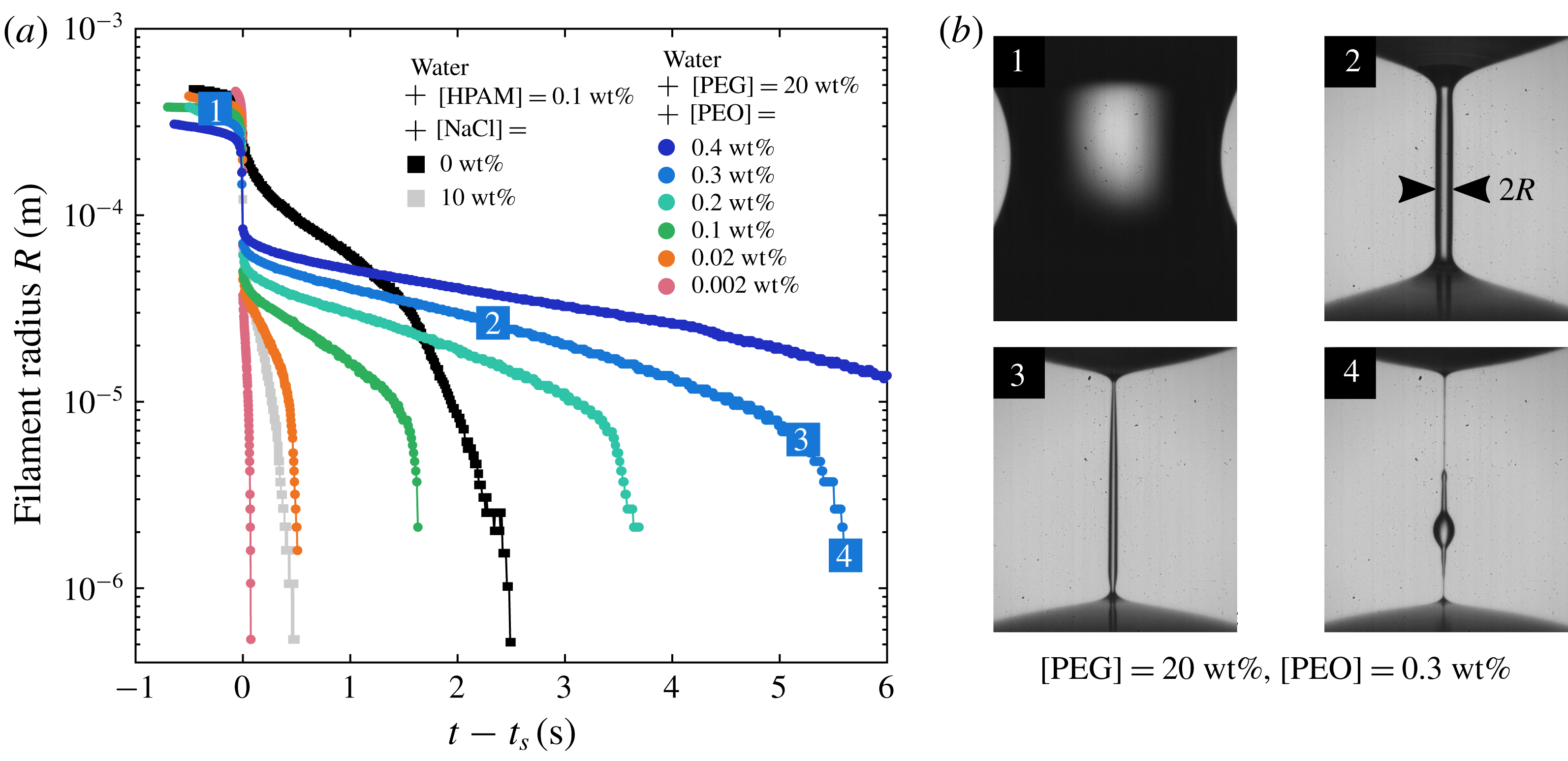
Figure 5 shows the evolution of the minimum filament radius
 $R$
as a function of time
 $t$
for PEO and HPAM solutions, along with raw images at four stages of thinning. Solutions are tested at room temperature
 $T=20\,^{\circ }\text{C}$
. Each filament undergoes the following steps. First (step 1 in figure 5
b), the liquid bridge slowly necks until abruptly transitioning to a slender filament shape (step 2). During this transition, elastic stresses become dominant due to rapid stretching of polymer molecules (Amarouchene et al.
Reference Amarouchene, Bonn, Meunier and Kellay2001). The filament then thins exponentially, as predicted from the multimode FENE-P model which gives (Entov & Hinch Reference Entov and Hinch1997)
 $$\begin{eqnarray}R(t)/\bar{R}_{0}=(G\bar{R}_{0}/2\unicode[STIX]{x1D6FE})\exp (-t/3\unicode[STIX]{x1D70F}_{1}),\end{eqnarray}$$
where
 $G$
is the elastic modulus,
 $\unicode[STIX]{x1D70F}_{1}$
is the longest relaxation time of the spectrum and
 $\bar{R}_{0}$
is the minimum filament radius after cessation of stretching in the classical step-strain plate separation protocol (Anna & McKinley Reference Anna and McKinley2001). The exponential regime is fitted by
 $R(t)\propto \exp (-t/3\unicode[STIX]{x1D70F}_{fil})$
where we define
 $\unicode[STIX]{x1D70F}_{fil}$
as the liquid extensional relaxation time. In this regime, the polymer chains undergo progressive unravelling under homogeneous uniaxial elongational flow with constant extension rate
 $\dot{\unicode[STIX]{x1D716}}\equiv -(2\,\text{d}R/\text{d}t)/R=2/3\unicode[STIX]{x1D70F}_{fil}$
. The filament remains perfectly cylindrical until polymer chains reach their maximum extension, allowing local pinching that typically occurs near the end drops (step 3). The filament then undergoes a Rayleigh–Plateau-like instability commonly referred to as ‘blistering instability’ (Sattler, Wagner & Eggers Reference Sattler, Wagner and Eggers2008; Sattler et al.
Reference Sattler, Gier, Eggers and Wagner2012; Eggers Reference Eggers2014) where tiny drops are separated by micrometric sub-filaments (step 4). In steps 3 and 4,
 $R$
refers to the radius of the pinched region and to the radius of the sub-filaments respectively.
Repeating this experiment for a given liquid shows reproducible results for PEO and salted HPAM solutions. We checked that experimental parameters such as the rate of plate separation had no impact on the measured value of
 $\unicode[STIX]{x1D70F}_{fil}$
, as also reported by Miller, Clasen & Rothstein (Reference Miller, Clasen and Rothstein2009) for polymer solutions. However, unsalted HPAM solutions showed less reproducible results. One possible explanation is that solutions of rigid polymers are analogous to particle suspensions which are known to be affected by random fluctuations in the particle concentration along the filament (McIlroy & Harlen Reference McIlroy and Harlen2014; Mathues et al.
Reference Mathues, McIlroy, Harlen and Clasen2015). Values of
 $\unicode[STIX]{x1D70F}_{fil}$
are reported in table 1 with a number of significant digits which reflects the precision of the measurement.
Considering a perfectly cylindrical filament with negligible inertia and gravity, the Laplace pressure
 $\unicode[STIX]{x1D6FE}/R$
is balanced by both solvent and polymeric stresses. The force balance equation writes
 $3\unicode[STIX]{x1D702}_{s}\dot{\unicode[STIX]{x1D716}}+(\unicode[STIX]{x1D70E}_{p,zz}-\unicode[STIX]{x1D70E}_{p,rr})=\unicode[STIX]{x1D6FE}/R$
where
 $\unicode[STIX]{x1D70E}_{p,zz}$
and
 $\unicode[STIX]{x1D70E}_{p,rr}$
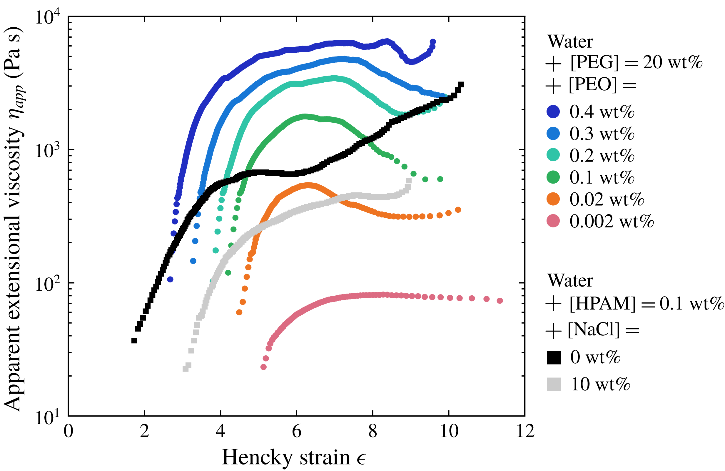
denote the axial and radial components of polymeric stresses. Defining the apparent extensional viscosity as
 $\unicode[STIX]{x1D702}_{app}\equiv (\unicode[STIX]{x1D70E}_{zz}-\unicode[STIX]{x1D70E}_{rr})/\dot{\unicode[STIX]{x1D716}}=3\unicode[STIX]{x1D702}_{s}+(\unicode[STIX]{x1D70E}_{p,zz}-\unicode[STIX]{x1D70E}_{p,rr})/\dot{\unicode[STIX]{x1D716}}$
, it can therefore be estimated using
 $$\begin{eqnarray}\unicode[STIX]{x1D702}_{app}=-\unicode[STIX]{x1D6FE}/(2\,\text{d}R/\text{d}t).\end{eqnarray}$$
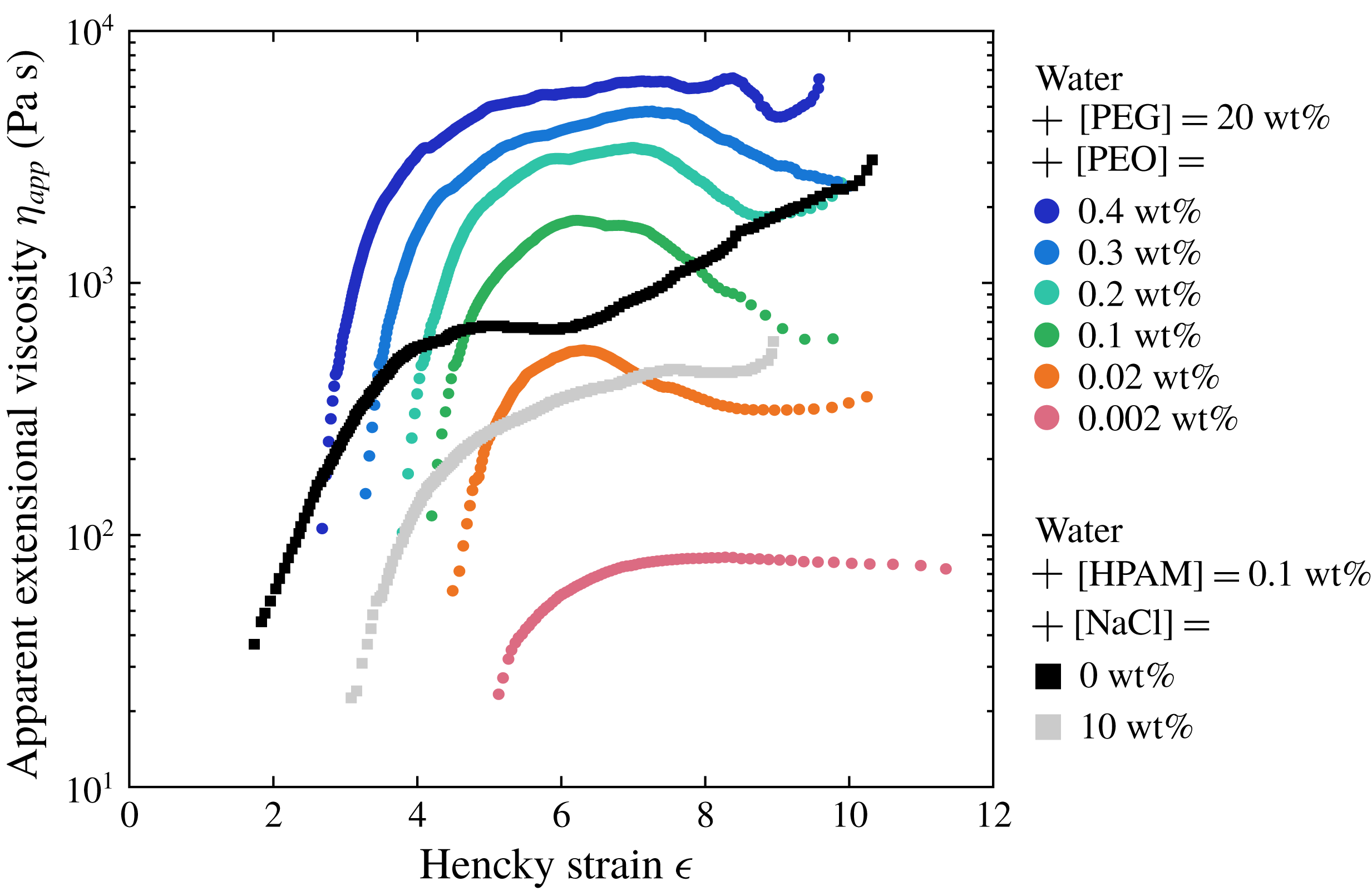
Figure 6 shows
 $\unicode[STIX]{x1D702}_{app}$
as a function of the total deformation accumulated by fluid elements, which is given by the Hencky strain
 $$\begin{eqnarray}\unicode[STIX]{x1D716}(t)\equiv \int _{0}^{t}\dot{\unicode[STIX]{x1D716}}(t^{\ast })\,\text{d}t^{\ast }=-2\ln [R(t)/R_{0}],\end{eqnarray}$$
where
 $R_{0}$
is the minimum bridge radius when the bridge starts necking. Finitely extensible nonlinear elastic (FENE) dumbbell models predict that
 $\unicode[STIX]{x1D702}_{app}$
reaches a plateau value known as the terminal extensional viscosity
 $\unicode[STIX]{x1D702}_{E}$
when polymer chains are fully extended (Bird et al.
Reference Bird, Armstrong, Hassager and Curtiss1987). It can be written as
 $\unicode[STIX]{x1D702}_{E}=3\unicode[STIX]{x1D702}_{s}+2b\unicode[STIX]{x1D702}_{p}$
(McKinley Reference McKinley2005) where
 $b^{1/2}$
is the ratio of the polymer size at full extension to its size in the coiled state at equilibrium, or equivalently
 $b=3N_{K}$
where
 $N_{K}$
is the number of Kuhn steps of the chain (Tirtaatmadja, McKinley & Cooper-White Reference Tirtaatmadja, McKinley and Cooper-White2006). Knowing
 $\unicode[STIX]{x1D702}_{s}$
and
 $\unicode[STIX]{x1D702}_{p}$
from shear measurements and estimating
 $\unicode[STIX]{x1D702}_{E}$
from extensional measurements, we estimate
 $b$
using
 $b=(\unicode[STIX]{x1D702}_{E}-3\unicode[STIX]{x1D702}_{s})/(2\unicode[STIX]{x1D702}_{p})$
as a definition. Of course, for semi-dilute solutions,
 $b$
has to be seen as an effective value since the FENE models do not take into account any chain–chain interaction. Values of
 $\unicode[STIX]{x1D702}_{E}$
and
 $b$
are reported in table 1. The finite extensibility parameter
 $b$
ranges between
 $10^{3}$
and
 $10^{5}$
for flexible PEO and salted HPAM solutions but is only of order
 $10^{0}{-}10^{1}$
for semi-rigid unsalted HPAM solutions.
3.3 Interpretation of the rheological data
Values of the critical overlap concentration
 $c^{\ast }$
can be calculated from the data of table 1 and estimated from theoretical expressions. A detailed discussion is presented in § A.1 and values of
 $c/c^{\ast }$
are reported in table 1, where
 $c=\unicode[STIX]{x1D70C}\text{[X]}$
(X refers to PEO or HPAM). In § A.2, we compare the CaBER extensional relaxation time
 $\unicode[STIX]{x1D70F}_{fil}$
and the shear relaxation time
 $\unicode[STIX]{x1D6F9}/2\unicode[STIX]{x1D702}_{p}$
. Values of the relaxation time and of the finite extensibility parameter
 $b$
are compared to theoretical expressions and some scalings are extracted from the data of table 1.


3.4 Mechanical degradation of polymer solutions and adequate protocols
During preparation (see § 2.1) of a 5 kg curtain solution, degradation of the polymer chains may occur during shaking since mechanical stirrers produce high shear rates. This is particularly true for PEO solutions since we measured that the relaxation time of two independently prepared solutions of same PEO concentration could vary by a factor of up to 3 (while HPAM solution are much more reproducible). Note that authors working with smaller samples use generally more gentle techniques such as magnetic stirrers or roller mixers which require longer preparation times. Hence the rheological data presented in the previous sections, which correspond to specific solutions with a particular preparation history, cannot be used as a reference for all other solutions. Therefore, rheological measurements are performed on any new solution.
Mechanical degradation of the polymer chains also occur in the hydraulic loop described in § 2.2. Irreversible scission of the polymer molecules occurs at each passage through the pump (which was found to be the principal source of degradation) and the rheological properties of the solution hence vary with time. Therefore, it would be incorrect to correlate curtain data with the rheological properties of the initial fresh solutions. In order to overcome this problem, we use two different experimental protocols.
For the first protocol, we take advantage of degradation by proceeding as follows. A newly prepared solution is placed in the reservoir and the pump is turned on at time
 $t_{d}=0$
. Filling the loop and setting the desired flow rate takes about 1 min. A first PIV measurement is performed, and we immediately collect a sample of the solution from the die. Without changing any external parameter, this procedure is repeated at times
 $t_{d}=10$
, 20, 40, 60 and 100 min. We therefore obtain six velocity profiles
 $U(z)$
corresponding to six degradation degrees of a given initial solution, which can be unambiguously correlated to the rheological properties of the six corresponding samples. For simplicity, the solution corresponding to the first measurement is called the fresh solution and is referred to as
 $t_{d}=0$
. Note that the flow rate
 $Q$
has to be regularly readjusted because it increases naturally over time due to a decreasing dissipation in the slot.
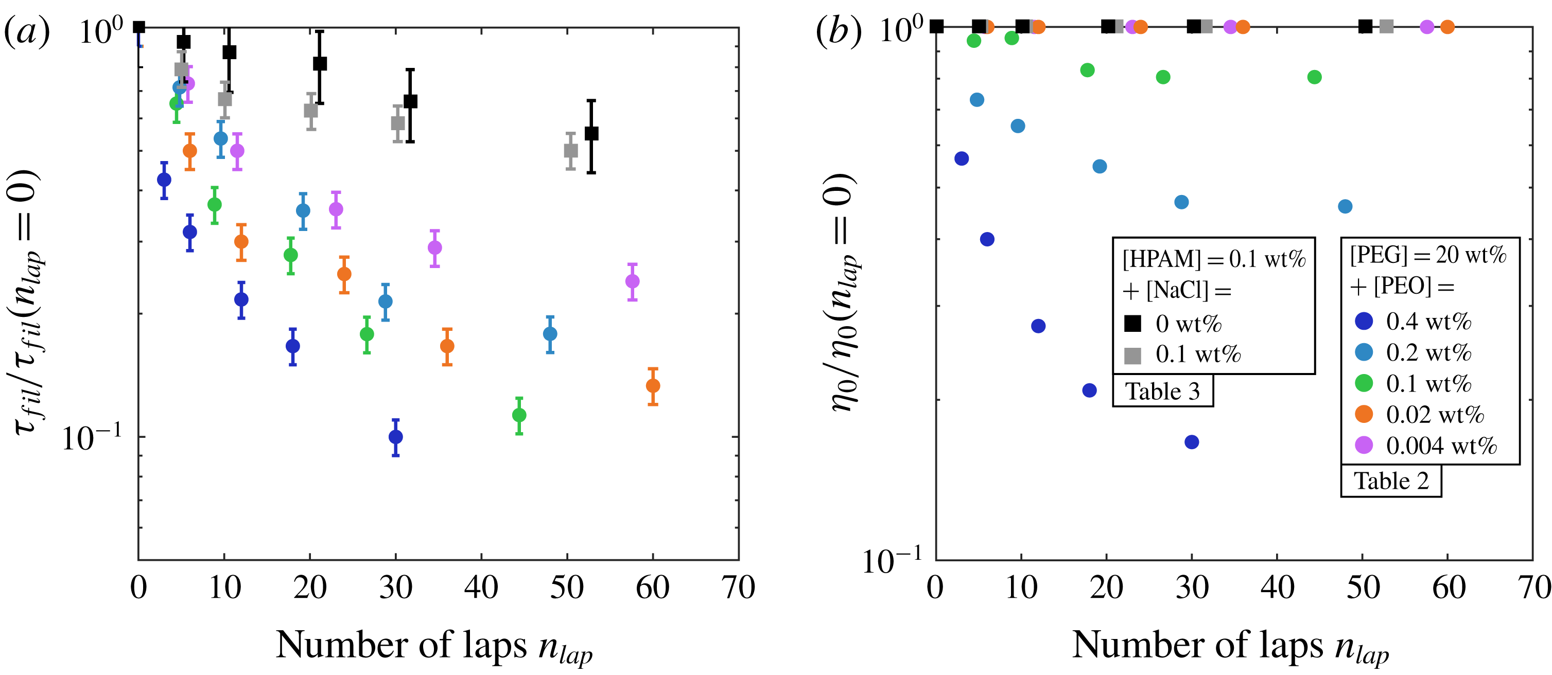
Dependence of the extensional relaxation time
 $\unicode[STIX]{x1D70F}_{fil}$
(a) and of the zero-shear viscosity
 $\unicode[STIX]{x1D702}_{0}$
(b) on the number of laps
 $n_{lap}$
through the hydraulic loop for PEO solutions with 20 wt% PEG solvent (table 2) and for HPAM solutions (table 3 (top));
 $n_{lap}$
is estimated by
 $t_{d}Q/M$
where
 $t_{d}$
is the time spent since the start of the experiment,
 $Q$
is the mass flow and
 $M=5~\text{kg}$
is the mass of the solution. Since solutions are extruded at different flow rates (see § 2.5), values at a given time
 $t_{d}$
correspond to different values of
 $n_{lap}$
. For each liquid,
 $\unicode[STIX]{x1D70F}_{fil}$
and
 $\unicode[STIX]{x1D702}_{0}$
are normalised by the initial values before degradation, i.e. at
 $t_{d}=0$
.
For a solution of total mass
 $M=5~\text{kg}$
flowing with mass flow
 $Q$
, the number of laps through the loop is
 $n_{lap}\approx t_{d}Q/M$
. We show in figure 7 the extensional relaxation time
 $\unicode[STIX]{x1D70F}_{fil}$
(a) and the zero-shear viscosity
 $\unicode[STIX]{x1D702}_{0}$
(b) as a function
 $n_{lap}$
for PEO solutions with 20 wt% PEG solvent and for HPAM solutions. Values are normalised by the initial value at
 $t_{d}=0$
. For PEO solutions,
 $\unicode[STIX]{x1D70F}_{fil}$
decreases by a factor of up to 10 after
 $100$
min. of circulation. In contrast, HPAM chains are more resistant since they deteriorate at a much lower rate. Besides, we observe that
 $\unicode[STIX]{x1D702}_{0}$
only decreases for PEO solutions which exhibit shear-thinning behaviour.
The detailed rheological parameters of all the solutions presented in figure 7 are given in tables 2 and 3 (top) (see appendix B). Shear-thinning PEO solutions become less shear thinning during degradation. Note that an extra HPAM solution is presented in table 3 (bottom); starting from a fresh unsalted HPAM solution, five PIV measurements are performed at arbitrary times, each measurement corresponding to a particular salt concentration which is achieved by adding salt to the solution. Samples are again collected at each step and rheological measurements are performed on each sample.
A second protocol is used when investigating the role of external parameters such as the curtain length (§ 4.3), the flow rate (§ 4.4) or the die geometry (§ 6.3). In this case, solutions must have the exact same rheological properties for each measurement. Instead of using the peristaltic pump, the liquid is poured manually from a bucket directly into a tank placed at two metres above the die and drilled with a hole on its lower side. A constant flow rate is ensured by keeping a constant liquid level in the tank. This degradation-free protocol was used with the PEO solutions with 40 wt% PEG solvent presented in table 4 (which have a fairly constant shear viscosity and large extensional relaxation times), and with the PEO solution of table 5 (see appendix B). We checked that the rheological parameters were the same before and after an experiment.
Curtain experiments are performed at room temperature, which could vary between
 $20\,^{\circ }\text{C}$
and
 $30\,^{\circ }\text{C}$
from day to day. Since temperature is not imposed in our ‘home made’ CaBER rheometer, the extensional rheology measurements are always performed a few minutes after curtain experiments and in the same room to measure the relevant extensional parameters. For the liquids of tables 4 and 5, the temperature of the curtain room was imposed for shear rheology measurements. However, for the liquids of tables 2 and 3, shear rheology measurements were performed at a temperature
 $T=20\,^{\circ }\text{C}$
which was not necessarily the room temperature. We measured on similar solutions that the variation of the viscosity parameters
 $\unicode[STIX]{x1D702}_{0}$
,
 $n$
and
 $\dot{\unicode[STIX]{x1D6FE}}_{c}$
is very weak within this temperature range (the zero-shear viscosity
 $\unicode[STIX]{x1D702}_{0}$
typically decreases by a factor of only 1.1 when raising the temperature from
 $20\,^{\circ }\text{C}$
to
 $30\,^{\circ }\text{C}$
, while
 $n$
and
 $\dot{\unicode[STIX]{x1D6FE}}_{c}$
remain unchanged). Hence, we can reasonably use the
 $20\,^{\circ }\text{C}$
values reported in tables 2 and 3. However, values of the first normal stress difference could vary significantly (by a factor 2). Hence, values of
 $\unicode[STIX]{x1D6FC}_{1}$
and
 $\unicode[STIX]{x1D6F9}$
are only reported for the liquids of tables 4 and 5. These values will be used for investigating die swell (§§ 4.6 and 6.1) and the impact of die geometry on the curtain flow (§ 6.3).
4 Observations
4.1 A dramatic shift towards sub gravity accelerations
Square
 $U^{2}$
of the falling velocity as a function of the distance
 $z$
from the slot for two Newtonian curtains [1] and [3], a 20 wt% PEG solution and pure glycerin of viscosities
 $\unicode[STIX]{x1D702}=0.017~\text{Pa}~\text{s}$
and
 $\unicode[STIX]{x1D702}=1.5~\text{Pa}~\text{s}$
respectively, and for a fresh (
 $t_{d}=0~\text{min}$
) 0.2 wt% PEO solution [2] with 20 wt% PEG solvent of zero-shear viscosity
 $\unicode[STIX]{x1D702}_{0}=0.12~\text{Pa}~\text{s}$
(table 2). The curtain length is
 $L_{c}=30~\text{cm}$
and the initial velocity
 $U_{1}$
at
 $z_{1}\approx 2.5~\text{mm}$
from the slot exit is
 $0.2~\text{m}~\text{s}^{-1}$
,
 $0.13~\text{m}~\text{s}^{-1}$
and
 $0.07~\text{m}~\text{s}^{-1}$
for liquids [1], [2] and [3] respectively. The local acceleration of the liquid is
 $U\,\text{d}U/\text{d}z$
.

To identify the specificity of polymer solutions in the context of curtain flows, we have performed a first series of experiments with three different liquids. The first one [1] is the Newtonian 20 wt% PEG solvent of viscosity
 $\unicode[STIX]{x1D702}=0.017~\text{Pa}~\text{s}$
. The second one [2] is a fresh (
 $t_{d}=0$
) 0.2 wt% PEO solution with 20 wt% PEG solvent (table 2). Its zero-shear viscosity is
 $\unicode[STIX]{x1D702}_{0}=0.12~\text{Pa}~\text{s}$
, ten times larger than the pure solvent [1]. The third one [3] is pure glycerin, a Newtonian liquid with a measured viscosity
 $\unicode[STIX]{x1D702}=1.5$
Pa s, a hundred times larger than the shear viscosity of liquid [1], and density
 $\unicode[STIX]{x1D70C}=1250~\text{kg}~\text{m}^{-3}$
. Note that we used a different setup for glycerin since, due to a strong viscous dissipation in the hydraulic loop, the maximum accessible flow rate is well below the minimum flow rate required to create a continuous curtain. Glycerin is placed in a reservoir connected to the die and a large enough flow rate is enforced by applying a constant air flow on the top of the reservoir.
In figure 8, we plot the square
 $U^{2}$
of the falling velocity of these liquids as a function of the distance
 $z$
from the slot. All three curtains have the same length
 $L_{c}=30~\text{cm}$
and start from comparable initial velocities
 $U_{1}$
ranging between
 $0.07~\text{m}~\text{s}^{-1}$
for glycerin [3] and
 $0.2~\text{m}~\text{s}^{-1}$
for the PEG solvent [1]. We recall that
 $U_{1}=U(z_{1})$
is the liquid velocity at
 $z_{1}\approx 2.5~\text{mm}$
from the slot exit (see § 2.4) while
 $U_{0}=U(z=0)$
is the liquid velocity at the slot exit. The local acceleration of the liquid is given by
 $U\,\text{d}U/\text{d}z$
which is half the local slope of the
 $U^{2}(z)$
curve. For both Newtonian curtains [1] and [3], we observe that this acceleration is equal to
 $g$
far from the slot exit. More precisely, the fall of the low viscosity Newtonian liquid [1] is very well captured by a free fall, i.e.
 $U^{2}=U_{0}^{2}+2gz$
, whereas the acceleration of glycerin reaches the asymptotic value
 $g$
at about 10 cm from the slot. These results are in agreement with the theory of viscous Newtonian curtains (1.1) according to which viscous forces are negligible far downstream from the slot. Indeed, the length of the sub-gravitational part of the flow is of order
 $z_{v}=((4\unicode[STIX]{x1D702}/\unicode[STIX]{x1D70C})^{2}/g)^{1/3}$
(1.2), respectively 0.077 cm and 1.4 cm for liquids [1] and [3], with a prefactor which is approximately 7 for low initial velocities
 $U_{0}\ll \sqrt{gz_{v}}$
(Brown Reference Brown1961; Clarke Reference Clarke1968). For glycerin, we measured
 $U_{0}=0.05~\text{m}~\text{s}^{-1}$
which gives
 $U_{0}/\sqrt{gz_{v}}\approx 0.14<1$
. Hence, according to the theory, the length of the sub-gravitational part of the flow should be approximately
 $7z_{v}\approx 10~\text{cm}$
which is in agreement with the experimental results.
In contrast, the PEO solution falls at much lower velocities than the two others, despite the fact that its zero-shear viscosity is one order of magnitude smaller than the viscosity of glycerin. More precisely, the acceleration at
 $z=14~\text{cm}$
from the slot is
 $U\,\text{d}U/\text{d}z=2.5~\text{m}~\text{s}^{-2}<g$
despite the fact that the viscous length
 $z_{v}=((4\unicode[STIX]{x1D702}_{0}/\unicode[STIX]{x1D70C})^{2}/g)^{1/3}$
is only 0.28 cm based on the zero-shear viscosity. Therefore, viscoelastic curtain flows are not captured by the Newtonian curtain theory.
4.2 Unstable flow for the most shear-thinning solutions
Example of PIV measurement for a degraded (
 $t_{d}=20~\text{min}$
) 0.1 wt% unsalted HPAM solution (table 3). (a) Superposition of six successive PIV images. The correlation algorithm is applied to a domain restricted to the dashed rectangle. (b)
 $z$
-component of the velocity field, i.e.
 $U(x,z,t)$
, against the horizontal coordinate
 $x$
at different distances
 $z$
from the slot at an arbitrary time
 $t$
. The curtain length is
 $L_{c}=30~\text{cm}$
and the linear flow rate is
 $q=3.1~\text{cm}^{2}~\text{s}^{-1}$
.
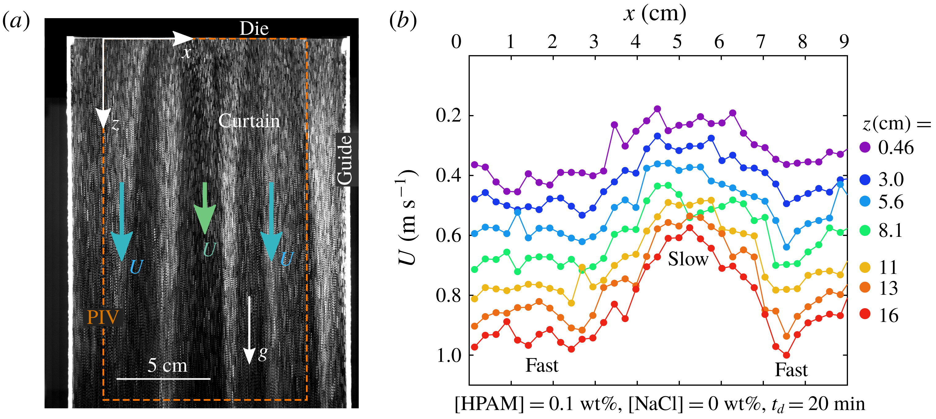
We mention here that the curtain flow is not always stationary and translation invariant in the
 $x$
horizontal direction (like in figure 2). Indeed, for some solutions, the curtain flow is unstable and presents a time-dependent varicose mode along
 $x$
, i.e. the velocity of the liquid and the curtain thickness depend on
 $x$
. This is illustrated by the vertical dark and bright stripes in figure 9(a) for an unsalted HPAM solution (bright and dark stripes correspond to flow regions with velocities respectively larger and smaller than the average velocity). This is one of the most extreme cases of unstable curtain flow. The wavelength and the typical time of evolution of the pattern are of the order of a few centimetres and a few tens of seconds, respectively. The corresponding velocity field
 $U(x,z,t)$
is presented in figure 9(b) at an arbitrary time
 $t$
. For example, at a distance
 $z=16~\text{cm}$
from the slot, the liquid velocity ranges between
 $0.6~\text{m}~\text{s}^{-1}$
and
 $1~\text{m}~\text{s}^{-1}$
which corresponds to a variation of
 $\pm 25\,\%$
around the average value
 $\langle U\rangle _{x}=0.85~\text{m}~\text{s}^{-1}$
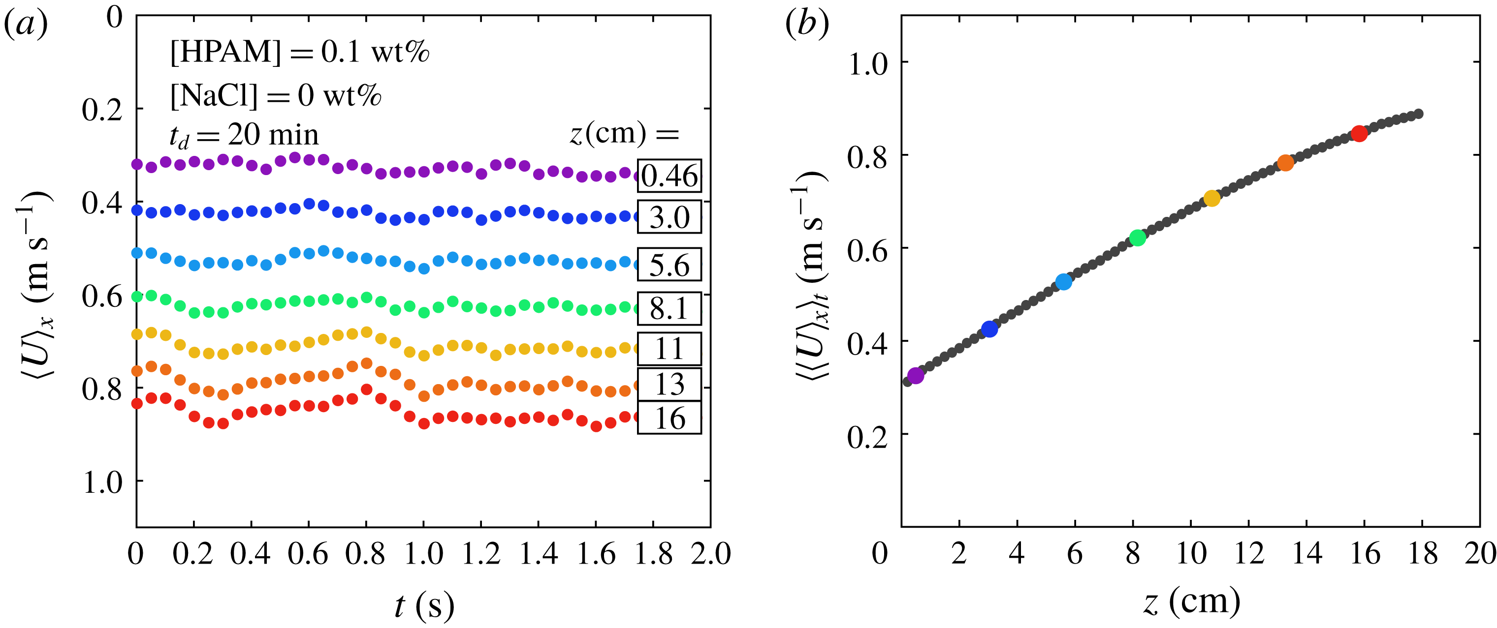
. The time variation of the average velocity
 $\langle U\rangle _{x}$
is presented in figure 10(a): it is fairly independent of time. Hence, we can reasonably define an average flow
 $U(z)=\langle \langle U\rangle _{x}\rangle _{t}$
obtained after averaging
 $\langle U\rangle _{x}$
over time, as presented in figure 10(b).
(a) Velocity
 $\langle U\rangle _{x}$
averaged over
 $x$
versus time
 $t$
(for a 2 s PIV movie) and at different distances
 $z$
from the slot. Time
 $t=0~\text{s}$
corresponds to the data of figure 9(b). (b) Velocity
 $\langle \langle U\rangle _{x}\rangle _{t}$
averaged over
 $x$
and
 $t$
versus
 $z$
. The big coloured dots correspond to the values of (a).
As salt is added to an initially unsalted HPAM solution, the amplitude of the instability decreases. It disappears for [NaCl]
 ${\geqslant}1$
wt%. Besides, for PEO solutions with 20 wt% PEG solvent (table 2), the curtain flow is weakly unstable for the highest concentration [PEO]
 $=$
0.4 wt%. However, as the polymer chains break due to mechanical degradation, the amplitude of the velocity variation decreases. It disappears for
 $t_{d}\geqslant 40~\text{min}$
. All other solutions in table 2 produce a stable curtain, as well as every PEO solution with 40 wt% PEG solvent (table 4). In this paper, whatever the curtain, stable or unstable, we focus on the mean flow
 $U(z)=\langle \langle U\rangle _{x}\rangle _{t}$
.
Here is more information on this instability, see Gaillard (Reference Gaillard2018) for details. Visualisations using a transparent die reveal that it appears to be generated at the contraction upstream of the slot. It is known that viscoelastic liquids can exhibit interesting nonlinear dynamics in both axisymmetric and planar contraction flows depending on the value of the Reynolds and Weissenberg number
 $\mathit{Wi}$
(McKinley et al.
Reference McKinley, Raiford, Brown and Armstrong1991; Purnode & Crochet Reference Purnode and Crochet1996; Rothstein & McKinley Reference Rothstein and McKinley1999; Nigen & Walters Reference Nigen and Walters2002; Boger & Walters Reference Boger and Walters2012). Using the definition of Rodd et al. (Reference Rodd, Scott, Boger, Cooper-White and McKinley2005, Reference Rodd, Scott, Cooper-White, Boger and McKinley2007)
 $\mathit{Wi}=\unicode[STIX]{x1D70F}_{fil}U_{s}/a$
, the maximum value attained in our experiments is
 $\mathit{Wi}=400$
. For solutions which are not too shear thinning, we observe the presence of small corner and lip vortices, as well as divergent streamlines at high flow rates, but no instabilities. Both phenomena are well documented. Within our experimental range of rheological parameters and flow rates, the only solutions producing a modulated curtain have a degree of shear thinning
 $n<0.72$
or, equivalently, an effective finite extensibility
 $b<3\times 10^{3}$
. For these solutions, the flow upstream of the contraction plane is unsteady, asymmetric and three dimensional. For unsalted HPAM solutions, we observe jet-like structures of fast portions of liquid moving in a much slower surrounding, thus leading to the curtain modulation along
 $x$
(thick and fast bands of liquid in the curtain correspond to overfed regions upstream of the slot). Three dimensional destabilisation of a planar contraction flow of polymer solution due to shear-thinning effects have also been reported by Chiba, Sakatani & Nakamura (Reference Chiba, Sakatani and Nakamura1990) and Chiba, Tanaka & Nakamura (Reference Chiba, Tanaka and Nakamura1992). However, to our knowledge, this particular instability and its consequences on the downstream curtain has not been mentioned in the literature. A more complete description and characterisation of this instability is left for a future work. Note that different scenarios leading to the destabilisation of viscoelastic liquid sheets have been investigated (Graham Reference Graham2003).
4.3 The influence of the curtain length
Velocity field
 $U(z)$
for
 $z\leqslant 32~\text{cm}$
for curtains of lengths
 $L_{c}$
ranging between 15 cm and 200 cm. The liquid falls onto a motionless horizontal plate (see inset on the right) and reaches a maximum velocity at a distance
 $z_{m}$
from the slot. The liquids are respectively 0.2 wt% (a) and 0.024 wt% (b) PEO solutions with 40 wt% PEG solvent (table 4). They are respectively extruded at flow rates
 $q=0.40~\text{cm}^{2}~\text{s}^{-1}$
and
 $0.98~\text{cm}^{2}~\text{s}^{-1}$
. The liquid velocity
 $U_{1}$
at
 $z_{1}\approx 2.5~\text{mm}$
from the slot is respectively
 $0.02~\text{m}~\text{s}^{-1}$
and
 $0.06~\text{m}~\text{s}^{-1}$
.
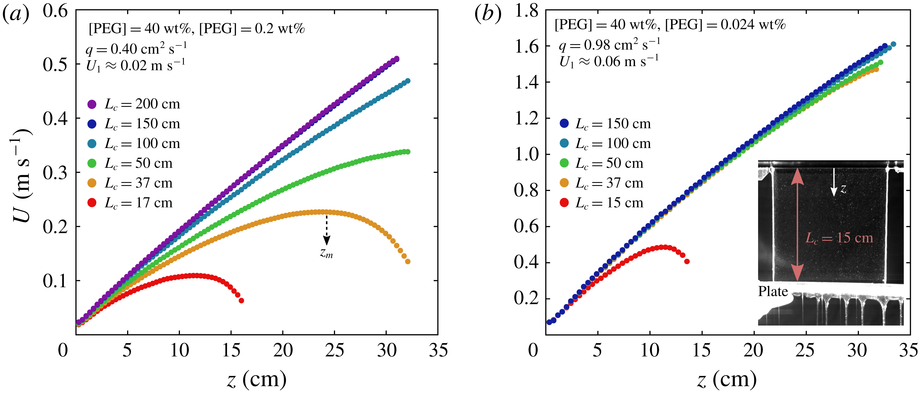
To investigate the role of the curtain length
 $L_{c}$
on the flow, we perform experiments with
 $L_{c}$
ranging from 15 cm to 200 cm. The experimental set-up is modified: after extrusion, the liquid is stopped at the desired distance
 $L_{c}$
from the slot by a horizontal plastic plate and finally falls into a reservoir. The vertical wires guiding the flow pass through two small holes drilled on the plastic plate to ensure that all the liquid is stopped. The camera only records the first 32 cm of the fall. Only the most elastic solutions could form a 2 m continuous curtain. On the other hand, curtains made of solutions with low polymer concentration usually break before reaching the plastic plate. Near the breaking zone, some curtains may even adopt a sinuous flag-like motion. We suspect that this is due to the shear instability with the surrounding air described by Dombrowski & Johns (Reference Dombrowski and Johns1963) and Villermaux & Clanet (Reference Villermaux and Clanet2002).
For these experiments, we use the PEO solutions with 40 wt% PEG solvent presented in table 4 along with the degradation-free protocol presented in § 3.4 to ensure that
 $L_{c}$
is the only varying parameter for a given solution. We only consider the curtains reaching the plastic plate without breaking. Some results are presented in figure 11 for [PEO]
 $=$
0.2 wt% (a) and [PEO]
 $=$
0.024 wt% (b). In the first case, longer curtains fall clearly faster than shorter ones, i.e. the velocity
 $U$
is larger at a any distance
 $z$
from the slot. The liquid vertical velocity has to vary from the imposed initial velocity
 $U(0)=U_{0}$
at the slot exit to
 $U(L_{c})=0$
when impinging onto the motionless plastic plate where the curtain flow turns into a plane stagnation flow. Everyday experience with jets of tap water suggests that the presence of a horizontal solid surface only affects the liquid flow within a few millimetres before impact. However, for the liquid of figure 11(a) with extensional relaxation time
 $\unicode[STIX]{x1D70F}_{fil}=1.1~\text{s}$
, the presence of the plate clearly affects the flow on a much larger scale: for
 $L_{c}=37~\text{cm}$
, the liquid velocity first increases and reaches a maximum value at
 $z=z_{m}\approx 25~\text{cm}$
before decreasing, i.e. the curtain starts to get thicker at a distance
 $L_{c}-z_{m}\approx 12~\text{cm}$
from the impact. As the plate is moved downwards, the flow field near the slot exit converges towards a universal behaviour which is no longer influenced by the presence of the plate: there is no difference between
 $L_{c}=150~\text{cm}$
and
 $L_{c}=200~\text{cm}$
within the first 32 cm of the fall in figure 11(a). This is even more visible for the solution used in figure 11(b) which has a lower extensional relaxation time
 $\unicode[STIX]{x1D70F}_{fil}=0.17~\text{s}$
since the liquid velocity
 $U(z)$
is almost the same for all curtain lengths, except for
 $L_{c}=15~\text{cm}$
.
4.4 The influence of the flow rate
(a) Velocity field
 $U(z)$
for the PEO solution of table 5 extruded at flow rates
 $q=0.45~\text{cm}^{2}~\text{s}^{-1}$
and
 $1.4~\text{cm}^{2}~\text{s}^{-1}$
. The liquid velocity
 $U_{1}$
at
 $z_{1}\approx 2.5~\text{mm}$
from the slot is respectively
 $0.047~\text{m}~\text{s}^{-1}$
and
 $0.082~\text{m}~\text{s}^{-1}$
. (b) Local acceleration
 $U\,\text{d}U/\text{d}z$
at an arbitrary distance
 $z=16~\text{cm}$
from the slot versus initial velocity
 $U_{1}$
. The curtain length is
 $L_{c}=50~\text{cm}$
.

To investigate the role of the flow rate, we perform experiments using the degradation-free protocol presented in § 3.4 to ensure that
 $q$
is the only varying parameter for a given solution. The test liquid is the PEO solution presented in table 5 which is close to (but not exactly the same as) the degraded (
 $t_{d}=100~\text{min}$
) 0.4 wt% PEO solution with 20 wt% PEG solvent presented in table 2. The liquid is extruded at different flow rates
 $q$
ranging between
 $0.45~\text{cm}^{2}~\text{s}^{-1}$
and
 $1.4~\text{cm}^{2}~\text{s}^{-1}$
. In figure 12(a), we report the velocity field
 $U(z)$
for these two flow rates;
 $U$
increases slightly faster when increasing the flow rate. To quantify this effect, values of the liquid acceleration
 $U\,\text{d}U/\text{d}z$
at an arbitrary distance
 $z=16~\text{cm}$
from the slot are reported in figure 12(b) as a function of the initial velocity
 $U_{1}$
measured at
 $z\approx 2.5~\text{mm}$
from the slot exit. The local acceleration is increased by a factor 1.2 when
 $U_{1}$
is increased by a factor 1.7. The same trend is observed for all solutions, including HPAM solutions (results not shown).
4.5 The influence of the rheological properties
To investigate the role of the rheological properties, we show in figure 13(a) the square
 $U^{2}(z)$
of the velocity field for the six 0.1 wt% PEO solutions with 20 wt% PEG solvent presented in table 2. These measurements are performed with the degradation protocol presented in § 3.4 and each solution corresponds to a specific degradation time. All six curtains share the same initial velocity
 $U_{1}\approx 0.17~\text{m}~\text{s}^{-1}$
at
 $z_{1}\approx 2.5~\text{mm}$
from the slot and the same curtain length
 $L_{c}=30~\text{cm}$
. These specific solutions are almost non-shear thinning (
 $n\approx 0.96$
) and have similar shear viscosities. In particular, the three last solutions have the same values of both
 $\unicode[STIX]{x1D702}_{0}=0.029~\text{Pa}~\text{s}$
and
 $\unicode[STIX]{x1D702}_{p}=0.012~\text{Pa}~\text{s}$
. However, we observe that the liquid acceleration increases with degradation time. This suggests that neither
 $\unicode[STIX]{x1D702}_{0}$
nor
 $\unicode[STIX]{x1D702}_{p}$
does fully control the curtain flow and that other rheological parameters are to be taken into account to rationalise the curtain data. The same conclusion can be drawn for the 0.02 wt% and 0.004 wt% PEO solutions of table 2 for which degradation has no impact on the shear viscosity (results not shown).
Dependence of the velocity field
 $U(z)$
on the rheological properties of the solution. (a)
 $U^{2}(z)$
for the 0.1 wt% PEO solutions with 20 wt% PEG solvent (table 2) for all degradation times
 $t_{d}=0$
to 100 min. All solutions are almost Boger fluids of comparable zero-shear viscosity
 $\unicode[STIX]{x1D702}_{0}\approx 0.03~\text{Pa}~\text{s}$
and have comparable initial velocities
 $U_{1}\approx 0.17~\text{m}~\text{s}^{-1}$
at
 $z_{1}\approx 2.5~\text{mm}$
from the slot. A free fall is shown for comparison. (b)
 $U^{2}(z)$
for five pairs of solutions [1], [2], [3], [4] and [5] from tables 2 and 3 (bottom) which are referred to as follows: [P0.2,
 $t_{d}\,60$
] corresponds to a 0.2 wt% PEO solution (with 20 wt% PEG solvent) with degradation time
 $t_{d}=60~\text{min}$
and [H0.1, salt 1] corresponds to a 0.1 wt% HPAM solution with salt concentration [NaCl]
 $=$
1 wt%. Within each pair, both solutions share similar initial velocities
 $U_{1}$
and comparable extensional relaxation times ranging between
 $\unicode[STIX]{x1D70F}_{fil}=0.0073{-}0.008~\text{s}$
[1] and
 $\unicode[STIX]{x1D70F}_{fil}=0.38{-}0.5~\text{s}$
[5]. The curtain length is
 $L_{c}=30~\text{cm}$
for both figures.

Dimensionless acceleration
 $[U\,\text{d}U/\text{d}z]/g$
at
 $z=18~\text{cm}$
from the slot against polymer extensional relaxation time
 $\unicode[STIX]{x1D70F}_{fil}$
in lin–lin (a) and log–log (b) scales for all the solutions of tables 2 (PEO) and 3 (HPAM), for which the curtain length is always
 $L_{c}=30~\text{cm}$
, and for all PEO the solutions of table 4 when the curtain length is also
 $L_{c}=30~\text{cm}$
. Note that another 0.4 wt% PEO solution with 20 wt% PEG solvent was prepared and that the curtain flow was measured at
 $t_{d}=0$
, 5, 10 and 20 min in order to fill the high relaxation time region of the curve.

In figure 13(b), we plot the square
 $U^{2}(z)$
of the velocity field for various PEO and HPAM solutions from tables 2 and 3 (bottom). The curtain length is
 $L_{c}=30~\text{cm}$
and we choose five pairs of solutions such that both solutions within each pair share comparable extensional relaxation times
 $\unicode[STIX]{x1D70F}_{fil}$
and initial velocities
 $U_{1}$
. The results suggest that the liquid fall is mostly influenced by the value of
 $\unicode[STIX]{x1D70F}_{fil}$
since the flow of both solutions within each pair is very similar. More precisely, the flow of solutions [1], which have low extensional relaxation times
 $\unicode[STIX]{x1D70F}_{fil}\approx 8~\text{ms}$
, is well captured by a free fall with constant acceleration
 $g=9.81~\text{m}~\text{s}^{-2}$
, whereas solutions with larger values of
 $\unicode[STIX]{x1D70F}_{fil}$
fall with an increasing sub-gravitational acceleration
 $U\,\text{d}U/\text{d}z(z)\leqslant g$
. These results are consistent with the recent results of Karim et al. (Reference Karim, Suszynski, Griffith, Pujari, Francis and Carvalho2018b
) who also measured free falls for curtains made of PEO solutions with extensional relaxation times
 $\unicode[STIX]{x1D70F}_{fil}\leqslant 7.3~\text{ms}$
.
Note that
 $\unicode[STIX]{x1D702}_{0}$
and
 $\unicode[STIX]{x1D702}_{p}$
vary significantly for the pair [3] in figure 13(b). This example reinforces the idea that shear viscosity does not fully control the curtain flow. The flexibility of the polymer chains also appears to play no major role since values of the effective finite extensibility
 $b$
(and of the degree of shear thinning
 $n$
) are very different for the solutions of pair [5]. To confirm these ideas, we gather all the data corresponding to
 $L_{c}=30~\text{cm}$
in figure 14 where the acceleration at a given (arbitrary) distance
 $z=18~\text{cm}$
from the slot is plotted against
 $\unicode[STIX]{x1D70F}_{fil}$
. We observe a good collapse of the data although neighbouring points in the plot can correspond to very different values of the other rheological parameters. This result confirms that curtain data can be fairly rationalised using only the extensional relaxation time
 $\unicode[STIX]{x1D70F}_{fil}$
measured from CaBER experiments. The deviations can be explained by the differences in flow rates: curtains extruded at lower flow rates have a slightly lower acceleration (§ 4.4). Note that some of the data in figure 14 correspond to the unstable curtains mentioned in § 4.2 and blend with the stable curtain data, which suggests that this instability does not affect significantly the average velocity field
 $U(z)=\langle \langle U\rangle _{x}\rangle _{t}$
.
According to figure 14(b), solutions with relaxation times
 $\unicode[STIX]{x1D70F}_{fil}\leqslant 10~\text{ms}$
have an acceleration
 $U\,\text{d}U/\text{d}z=g$
at
 $z=18~\text{cm}$
from the slot exit. In fact, for some of these solutions, the local liquid acceleration is less than
 $g$
close to the slot and reaches the free-fall value
 $g$
at
 $z<18~\text{cm}$
. This is reminiscent of the flow of pure glycerin reported in figure 8, which suggests that
 $g$
is also the asymptotic value of the liquid acceleration for viscoelastic curtains. However, due to the finite length of the curtain, many liquids are stopped before reaching the free-fall behaviour. This is particularly true for solutions with high relaxation times
 $\unicode[STIX]{x1D70F}_{fil}\approx 1~\text{s}$
which fall with very low accelerations
 $U\,\text{d}U/\text{d}z\approx 0.1~\text{m}~\text{s}^{-2}\ll g$
at
 $z=18~\text{cm}$
from the slot exit.
4.6 Die swell
We recall that the first value
 $U_{1}=U(z_{1})$
measured by PIV corresponds to the velocity at
 $z_{1}\approx 2.5~\text{mm}$
from the slot exit, whereas the mean velocity in the slot can be estimated as
 $U_{s}=q/2a$
where
 $q$
is the measured linear flow rate and
 $2a$
is the slot thickness. Values of both
 $U_{s}$
and
 $U_{1}$
are reported in tables 2–4 for the corresponding curtains experiments. We observe that
 $U_{1}$
is systematically smaller than
 $U_{s}$
, except for HPAM curtains, and that the ratio
 $\unicode[STIX]{x1D709}=U_{s}/U_{1}$
is up to 2 and increases with polymer concentration. Observations with the naked eye confirm that the curtain rapidly swells at the slot exit. This is not due to a wetting effect, as expected from the design of the die where the wall edges are bevelled (figure 1
b).
(a) Velocity field
 $U(z)$
at the slot exit measured from single particle tracking velocimetry (PTV) for the PEO solution of table 5 extruded at different flow rates
 $q$
ranging between
 $0.45$
and
 $1.4~\text{cm}^{2}~\text{s}^{-1}$
. The curtain swells since the mean velocity decreases from
 $U_{0}$
at
 $z=0$
to
 $U(z_{d})$
at a distance
 $z_{d}$
from the slot exit;
 $U_{0}$
is estimated by extrapolation the PTV data. The PIV velocity fields are also shown for comparison, the first value
 $U_{1}$
corresponding to
 $z_{1}\approx 2.5~\text{mm}$
. To guide the eye,
 $z_{1}$
,
 $z_{d}$
,
 $U_{0}$
,
 $U_{1}$
and
 $U(z_{d})$
are shown for the data corresponding to
 $q=1.4~\text{cm}^{2}~\text{s}^{-1}$
. (b) The corresponding values of
 $U_{0}$
and
 $U(z_{d})$
are plotted against the mean velocity
 $U_{s}=q/2a$
inside the slot.

In order to estimate the velocity profile
 $U(z)$
in this region, we can use the particle tracking velocimetry (PTV) technique within the first millimetres of the flow, i.e. we track the position of singles particles after leaving the slot. Image processing is performed ‘manually’. Results are presented in figure 15(a) for the PEO solution of table 5 extruded at different flow rates. The liquid velocity first decreases from
 $U_{0}=U(z=0)$
at the slot exit to a minimum value at
 $z=z_{d}$
before finally increasing, where
 $z_{d}$
increases from 1.5 to 4 mm when increasing the flow rate, which is reminiscent of the delayed die swell effect (Delvaux & Crochet Reference Delvaux and Crochet1990; Boger & Walters Reference Boger and Walters2012). PIV measurements are not able to capture this behaviour since cross-correlation is computed over millimetric windows. However, a superposition of the PIV velocity profiles in figure 15(a) shows an acceptable agreement between the first value
 $U_{1}$
measured from PIV and the minimum velocity
 $U(z_{d})$
measured from particle tracking:
 $U(z_{d})=U_{1}$
with less than 15 % error. The values of
 $U_{0}$
and
 $U(z_{d})$
are reported in figure 15(b) as a function of the mean velocity
 $U_{s}$
in the slot. As expected,
 $U_{0}=U_{s}$
. Besides, the swelling ratio
 $\unicode[STIX]{x1D709}=U_{s}/U(z_{d})$
increases when increasing the flow rate. In the following,
 $z_{d}$
and
 $U(z_{d})$
are approximated by
 $z_{1}$
and
 $U_{1}$
for the sake of simplicity.
5 Theoretical description of the curtain flow
5.1 General overview of the problem
Before focusing on the theoretical description of the curtain flow, we would like to give in this section a general overview of the different types of flows involved in this problem. We first provide a qualitative description before focusing specifically on Newtonian liquids and viscoelastic liquids. The liquid first experiences a planar contraction of ratio
 $A/a$
at the slot entrance (figure 1
b). The mean liquid velocity on the centre line
 $y=0$
switches from about
 $q/2A$
in the hollow box to
 $U_{s}=q/2a$
inside the slot in a characteristic time
 $a/U_{s}$
, where
 $q$
is the linear flow rate and
 $2a$
is the slot thickness. Then, a Poiseuille flow is established in the slot due to the development of a viscous boundary layer along the walls. At the slot exit, the wall boundary condition switches to a free-surface boundary condition, i.e. zero shear stress at the liquid–air interface. Hence, due to viscous diffusion, the Poiseuille flow switches to a plug flow, as illustrated in figure 16. Here
 $U$
is the mean vertical velocity averaged over the curtain thickness. After initial swelling at the slot exit, the curtain thickness decreases since fluid particles are now accelerated by gravity. Since the liquid may develop some resistance to gravitational forces, the local mean acceleration
 $U\,\text{d}U/\text{d}z$
may be initially less than
 $g$
. The asymptotic free-fall regime where
 $U\,\text{d}U/\text{d}z=g$
is reached when inertia overcomes the resistance of the liquid.
Sketch of an infinitely long viscoelastic curtain (cross-sectional view). During the swelling at the slot exit, the mean liquid velocity
 $U$
and the mean normal stress difference
 $\unicode[STIX]{x1D6E5}=\unicode[STIX]{x1D70E}_{zz}-\unicode[STIX]{x1D70E}_{yy}$
averaged over the curtain thickness switch respectively from
 $U_{s}$
and
 $\unicode[STIX]{x1D6E5}_{s}$
to
 $U_{1}$
and
 $\unicode[STIX]{x1D6E5}_{1}$
at
 $z_{1}\approx 2.5~\text{mm}$
from the slot exit. The local vertical velocity field
 $u(y,z)$
switches from a Poiseuille flow inside the slot to a plug flow at a distance
 $z=L_{e}^{\ast }$
from the slot. In parallel, the mean velocity field
 $U(z)$
is characterised by a transition from a sub-gravitational regime to an asymptotic free-fall regime at a distance
 $z=z_{e}^{\ast }$
from the slot.
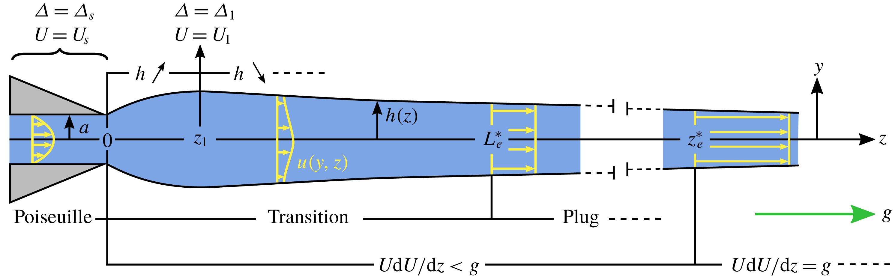
For Newtonian liquids, a fully developed Poiseuille flow is expected to be established after a distance from the entrance of the slot which scales as
 $L_{v}=\unicode[STIX]{x1D70C}U_{s}a^{2}/\unicode[STIX]{x1D702}=Re\,a$
with a prefactor typically less than one (Kays, Crawford & Weigand Reference Kays, Crawford and Weigand2005) where
 $Re=\unicode[STIX]{x1D70C}U_{s}a/\unicode[STIX]{x1D702}$
is the Reynolds number.
 $L_{v}$
is also the characteristic length scale of the transition from Poiseuille to plug. More precisely, the plug flow is fully established at a distance
 $L_{v}^{\ast }=P_{v}L_{v}$
from the slot, where
 $P_{v}$
is a dimensionless prefactor. In the case of axisymmetric laminar capillary jets, Sevilla (Reference Sevilla2011) shows that
 $P_{v}$
is a function of the Weber number
 $\mathit{We}=\unicode[STIX]{x1D70C}U_{s}^{2}a/\unicode[STIX]{x1D6FE}$
where
 $a$
is the injector radius, and gives
 $P_{v}(\mathit{We}=10)\approx 0.2$
. Furthermore, the mean acceleration effectively reaches the asymptotic free-fall value
 $g$
at a distance
 $z_{v}^{\ast }=F_{v}z_{v}$
(‘
 $v$
’ for ‘viscous’) from the slot where
 $z_{v}=((4\unicode[STIX]{x1D702}/\unicode[STIX]{x1D70C})^{2}/g)^{1/3}$
and where the prefactor
 $F_{v}$
is a decreasing function of the initial curtain velocity (Brown Reference Brown1961; Clarke Reference Clarke1968). In other words,
 $U\,\text{d}U/\text{d}z(z=z_{v}^{\ast })\approx g$
. Ignoring the prefactors, the ratio between the Poiseuille to plug and sub-gravitational to free-fall transition lengths is
 $$\begin{eqnarray}\frac{L_{v}}{z_{v}}=Re\frac{a}{z_{v}}=\frac{U_{s}a^{2}\unicode[STIX]{x1D70C}^{5/3}g^{1/3}}{4^{2/3}\unicode[STIX]{x1D702}^{5/3}},\end{eqnarray}$$
which means that liquids of large viscosity (
 $L_{v}/z_{v}\ll 1$
) exhibit a long sub-gravitational plug flow whereas liquids of low viscosity (
 $L_{v}/z_{v}\gg 1$
) fall with a mean acceleration
 $g$
while exhibiting velocity gradients along the thickness direction.
We now focus on the viscoelastic liquids used in our experiments. For all solutions, the time scale
 $a/U_{s}$
of the planar contraction is shorter than the extensional relaxation time
 $\unicode[STIX]{x1D70F}_{fil}$
. Hence, the polymer molecules undergo a rapid strain of Hencky strain
 $\unicode[STIX]{x1D716}\approx \ln (A/a)=2.6$
(3.5). Significant extensional stresses may arise due to this sudden polymer elongation. However, the time
 $L_{s}/U_{s}$
spent by the liquid inside the slot is generally longer than
 $\unicode[STIX]{x1D70F}_{fil}$
. Therefore, the polymeric stress developed by the liquid at the slot entrance is expected to relax towards the asymptotic Poiseuille flow value before leaving the slot. Moreover, since the Reynolds number ranges between 0.03 and 10 based on the zero-shear viscosity
 $\unicode[STIX]{x1D702}_{0}$
, the viscous length
 $L_{v}$
ranges between 0.01 mm and 5 mm which is much smaller than the slot length
 $L_{s}=10~\text{cm}$
. This suggests that a fully developed Poiseuille flow is established long before the slot exit, as confirmed by direct visualisation.
Using analogous notations for viscoelastic curtains, let
 $z_{e}^{\ast }$
(‘
 $e$
’ for ‘elastic’) be the distance from the slot at which the local acceleration of the liquid reaches the asymptotic value
 $g$
. We showed in §§ 4.1 and 4.5 that this transition length can be much larger than what could be expected from the theory of Newtonian curtains, i.e.
 $z_{e}^{\ast }\gg z_{v}^{\ast }$
, and that it was mainly determined by the value of the extensional relaxation time
 $\unicode[STIX]{x1D70F}_{fil}$
of the polymer solution. Of course, regardless of the liquid rheology, this discussion only makes sense if the curtain length is larger than this transition length, i.e.
 $L_{c}>z_{e}^{\ast }$
or
 $L_{c}>z_{v}^{\ast }$
, otherwise the curtain flow would turn into a plane stagnation flow before reaching the free-fall regime.
Direct visualisation of the
 $y$
dependence of the curtain flow is quite difficult. Therefore, to estimate the length
 $L_{e}^{\ast }$
at which the plug flow is fully established in the case of viscoelastic liquids, we visualised the flow of some PEO solutions when issuing from a nozzle of diameter 1 mm. For the degraded (
 $t_{d}=100~\text{min}$
) 0.1 wt% PEO solution with 20 wt% PEG solvent (table 2), we measure
 $L_{e}^{\ast }\approx 1.2~\text{cm}$
although the transition to free fall is out of frame in curtain experiments, i.e.
 $z_{e}^{\ast }>18~\text{cm}$
. Hence, provided that the order of magnitude of
 $L_{e}^{\ast }$
is comparable in the curtain, we can reasonably assume that the plug flow is established much sooner than the free-fall regime, i.e.
 $L_{e}^{\ast }/z_{e}^{\ast }\ll 1$
. We mention here that our measurements suggest an influence of elasticity on the Poiseuille to plug transition:
 $L_{e}^{\ast }$
is larger than what could be expected from the theory of Newtonian curtains. Further analysis is required to characterise this effect.
In this paper, we focus on the transition from the sub-gravitational regime to the free-fall regime. In particular, we wish to characterise the sub-gravitational regime in the case of a viscoelastic curtain and to express
 $z_{e}^{\ast }$
as a function of the parameters of the problem.
5.2 A master curve for Newtonian curtains
As we will now show, the velocity field
 $U(z)$
of an infinitely long Newtonian curtain collapses on a master curve which, to the best of our knowledge, had not been clearly identified in the literature so far. This analytical description of Newtonian curtains will be a useful guide when describing the analogous case of viscoelastic curtains.
In 1961, Taylor proposed in the appendix of Brown (Reference Brown1961) the one-dimensional force balance equation (1.1) for the steady curtain flow of a Newtonian liquid of density
 $\unicode[STIX]{x1D70C}$
and dynamic viscosity
 $\unicode[STIX]{x1D702}$
. Surface tension is neglected and the gas surrounding the liquid is assumed to be dynamically passive. This equation is valid for slender curtain, i.e.
 $\text{d}h/\text{d}z\ll 1$
where
 $2h$
is the curtain thickness. Aidun (Reference Aidun1987) and Ramos (Reference Ramos1996) derived this equation rigorously from a long-wave approximation of the Navier–Stokes equation using the aspect ratio
 $a/L_{c}\ll 1$
as a small parameter, where
 $2a$
and
 $L_{c}$
are respectively the slot thickness and the curtain length. Equation (1.1) can be put into non-dimensional form when rescaling by
 $$\begin{eqnarray}\left.\begin{array}{@{}c@{}}\bar{z}=z/z_{v},\\ \bar{U}=U/U_{v},\end{array}\right\}\quad z_{v}=\left(\frac{(4\unicode[STIX]{x1D702}/\unicode[STIX]{x1D70C})^{2}}{g}\right)^{1/3},\quad U_{v}=\sqrt{gz_{v}}=(4\unicode[STIX]{x1D702}g/\unicode[STIX]{x1D70C})^{1/3}.\end{eqnarray}$$
We obtain
 $$\begin{eqnarray}\bar{U}\bar{U}^{\prime }=1+\bar{U}^{\prime \prime }-\bar{U}^{\prime 2}/\bar{U},\end{eqnarray}$$
where
 $^{\prime }$
denotes spatial derivation
 $\text{d}/\text{d}\bar{z}$
. The general solution of this equation was found by Clarke (Reference Clarke1966, Reference Clarke1968) and is given by
 $$\begin{eqnarray}\bar{U}(\bar{z})=2^{-1/3}\left[\left(\frac{\text{Ai}^{\prime }(Z)+C\text{Bi}^{\prime }(Z)}{\text{Ai}(Z)+C\text{Bi}(Z)}\right)^{2}-Z\right]^{-1},\quad Z=2^{-1/3}(\bar{z}+k),\end{eqnarray}$$
where
 $\text{Ai}$
and
 $\text{Bi}$
are the Airy functions (Abramowitz & Stegun Reference Abramowitz and Stegun1964) and
 $C$
and
 $k$
are integration constants that are to be determined from the upstream and downstream boundary conditions. The upstream boundary condition is simply
 $$\begin{eqnarray}\bar{U}(\bar{z}=0)\equiv \bar{U}_{0}=U_{0}/U_{v}=\unicode[STIX]{x1D70C}U_{0}z_{v}/4\unicode[STIX]{x1D702},\end{eqnarray}$$
where the initial liquid velocity
 $U_{0}$
at the slot exit can be chosen experimentally by varying the flow rate. Three types of downstream boundary conditions can be chosen depending on the particular experimental conditions (Ramos Reference Ramos1996). As shown in figure 17(a), the type of downstream boundary condition depends on the value of
 $C$
in Clarke’s solution (5.4). Imposing an arbitrarily large velocity at a given distance
 $L_{c}$
from the slot corresponds to a film casting experiment where the liquid is collected by a drum rotating at a constant arbitrary angular velocity. This case corresponds to
 $C>0$
where Clarke’s solution diverges in finite time. On the other hand, the boundary condition
 $U(L_{c})=0$
leads to the transition to a plane stagnation flow where the liquid spreads onto a motionless horizontal solid plate placed at
 $z=L_{c}$
from the slot. In the latter case, which corresponds to
 $C<0$
, the liquid velocity first increases due to gravitational forces and reaches a maximum value at a distance
 $z_{m}$
from the slot before finally decreasing down to
 $0$
when approaching the stagnation point at
 $z=L_{c}$
. According to figure 17(a), the presence of the solid plate only affects the flow significantly within a distance from the plate which is of order
 $L_{c}-z_{m}$
. In figure 17(b), we present
 $\bar{L}_{c}-\bar{z}_{m}=(L_{c}-z_{m})/z_{v}$
against the dimensionless curtain length
 $\bar{L}_{c}=L_{c}/z_{v}$
for various initial velocities. These results suggest that
 $L_{c}-z_{m}$
is always less of equal to
 $2.3z_{v}$
. However, as pointed out by Ramos (Reference Ramos1996), the slender approximation is not justified near the stagnation point where the transverse velocity component becomes larger than the axial one. In this case, although solution (5.4) may be valid far enough from the impingement zone, a two-dimensional analysis is required when focusing on this zone. We can however reasonably assume that the presence of the solid plate only affects the flow within a distance before impact which is of order
 $z_{v}$
.
(a) Clarke’s solution (5.4) for
 $C=-10^{2}$
[1],
 $C=-10^{-1}$
[2],
 $C=-10^{-3.5}$
[3],
 $C=-10^{-7}$
[4],
 $C=-10^{-12}$
[5],
 $C=0$
[6] and
 $C=+10^{-12}$
[7], where
 $k$
is chosen to ensure that the initial velocity is
 $\bar{U}_{0}=10^{-3}$
for each curve. Solutions with
 $C<0$
,
 $C=0$
and
 $C>0$
correspond to different types of downstream boundary condition, respectively a plane stagnation flow for
 $C<0$
(where
 $\bar{U}(\bar{L}_{c})=0$
when impacting a flat solid plate at a distance
 $L_{c}=\bar{L}_{c}z_{v}$
from the slot), an infinite curtain which converges to a free fall for
 $C=0$
, and a film casting experiment for
 $C>0$
(where the velocity imposed by the rotation speed of the drum can be arbitrarily large). When
 $C<0$
, the presence of the solid plate only affects the flow within a (dimensionless) distance from the plate which is of order
 $\bar{L}_{c}-\bar{z}_{m}$
where
 $\text{d}\bar{U}/\text{d}\bar{z}(\bar{z}=\bar{z}_{m})=0$
. (b)
 $\bar{L}_{c}-\bar{z}_{m}$
against
 $\bar{L}_{c}$
for different initial velocities
 $\bar{U}_{0}$
. Since varying
 $k$
for a given
 $C$
only translates the curve along the
 $\bar{z}$
-axis in (5.4),
 $\bar{L}_{c}-\bar{z}_{m}$
does not depend on
 $k$
. Hence, all the curves in (b) corresponding to different values of
 $\bar{U}_{0}$
can be deduced from each other by simple translation along the
 $\bar{L}_{c}$
-axis.
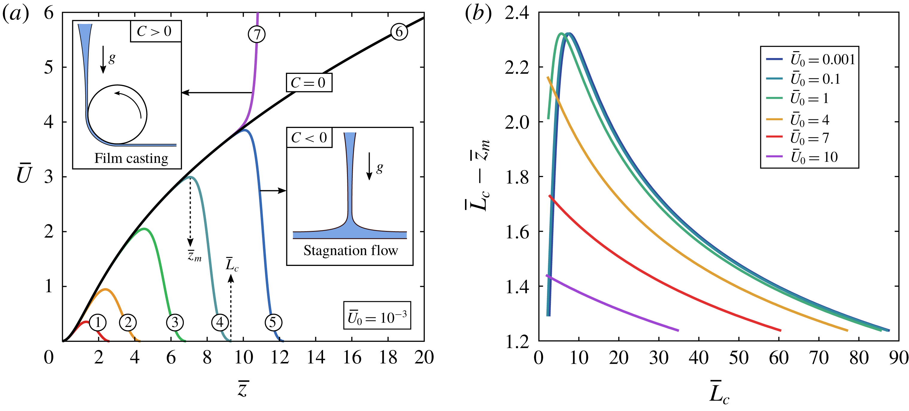
According to the previous results, if the curtains length is
 $L_{c}\gg z_{v}$
, the flow close to the slot is universal and is not influenced by the downstream boundary condition. Therefore, in order to characterise this universal flow far from the impingement zone, we can use the following boundary condition
 $$\begin{eqnarray}\lim _{\bar{z}\rightarrow \infty }\bar{U}\bar{U}^{\prime }=1,\end{eqnarray}$$
which ensures that the flow would converge asymptotically to a free fall with constant acceleration
 $g$
for a curtain of infinite length. This boundary condition corresponds to
 $C=0$
in solution (5.4) (figure 17
a). It is the case discussed by Clarke (Reference Clarke1966, Reference Clarke1968). In curtain coating, note that the liquid falls onto a horizontal solid surface moving horizontally at constant speed, which breaks the symmetry of the problem. However, we can reasonably assume that the flow far from the impingement zone is also not influenced by this boundary condition.
(a) Dimensionless velocity field
 $\bar{U}(\bar{z})$
for an infinitely long curtain made of a Newtonian liquid ((5.4) for
 $C=0$
), starting from various initial velocities
 $\bar{U}_{0}$
ranging between 0 and 2. All the curves for
 $\bar{U}_{0}>0$
collapse on the master curve
 $M_{v}$
corresponding to
 $\bar{U}_{0}=0$
after translation of each curve along the
 $\bar{z}$
axis by a distance
 $M_{v}^{-1}(\bar{U}_{0})$
(5.8). (b) Confirmation with the experimental velocity field of the pure glycerin curtain of figure 8 where
 $\bar{U}_{0}=0.14$
. The master curve
 $M_{v}$
is characterised by an initial (sub-gravitational) viscous regime and an asymptotic (free-fall) inertial regime (5.9).

Analytical solutions
 $\bar{U}(\bar{z})$
are shown in figure 18(a) for
 $C=0$
and initial velocities
 $\bar{U}_{0}$
ranging between 0 and 2. The curves are similar. In fact, they all rescale on a unique master curve after translation along the
 $\bar{z}$
axis. Indeed, let
 $M_{v}$
(‘
 $M$
’ for ‘Master curve’) be the particular solution corresponding to
 $\bar{U}_{0}=0$
. We have
 $$\begin{eqnarray}M_{v}(\bar{z})=2^{-1/3}\left[\left(\frac{\text{Ai}^{\prime }(Z)}{\text{Ai}(Z)}\right)^{2}-Z\right]^{-1},\quad Z=2^{-1/3}(\bar{z}+k_{0}),\end{eqnarray}$$
where
 $\text{Ai}(2^{-1/3}k_{0})=0$
which gives
 $k_{0}\approx -2.94583$
. Of course, achieving a curtain of zero initial velocity with infinite initial thickness is not physically possible. Yet, we can easily demonstrate that any physical solution with initial velocity
 $\bar{U}_{0}>0$
writes
 $$\begin{eqnarray}\bar{U}(\bar{z})=M_{v}(\bar{z}+M_{v}^{-1}(\bar{U}_{0})),\end{eqnarray}$$
where
 $M_{v}^{-1}$
is the functional inverse of
 $M_{v}$
. Indeed, since
 $\bar{z}$
does not appear explicitly in (5.3), if
 $M_{v}$
is a particular solution, then
 $\bar{z}\mapsto M_{v}(\bar{z}+\text{const.})$
is also a solution. Since expression (5.8) is the only one satisfying both the upstream (
 $\bar{U}(\bar{z}=0)=\bar{U}_{0}$
) and downstream (
 $\bar{U}\bar{U}^{\prime }\rightarrow 1$
) boundary conditions, it is the only solution. Hence, any solution
 $\bar{U}(\bar{z})$
with initial velocity
 $\bar{U}_{0}>0$
will collapse on the master curve
 $M_{v}(\bar{z})$
after translation along the
 $\bar{z}$
axis by a distance
 $M_{v}^{-1}(\bar{U}_{0})$
on the right. For the glycerin curtain in figure 8, we have
 $\bar{U}_{0}=0.14$
and
 $M_{v}^{-1}(\bar{U}_{0})=0.55$
. Therefore, shifting the dimensionless profile
 $\bar{U}(\bar{z})$
by a distance 0.55 on the right makes the experimental data collapse on the master curve, as shown in figure 18(b).
The master curve is characterised by two regimes:
 $$\begin{eqnarray}M_{v}(\bar{z})=\left\{\begin{array}{@{}ll@{}}\bar{z}^{2}/2\quad & \bar{z}\ll 1\text{: viscous regime},\\ \sqrt{2(\bar{z}-s_{v,0})}\quad & \bar{z}\gg 1\text{: inertial regime},\end{array}\right.\end{eqnarray}$$
where
 $s_{v,0}\approx 2.8$
. The initial viscous regime (
 $\bar{z}\ll 1$
) corresponds to a balance between gravity and viscous forces where inertia is negligible in (1.1). As the liquid velocity increases, we enter into an intermediate inertio-viscous regime where none of the terms of (1.1) can be neglected. Finally, inertia dominates over viscous forces for
 $\bar{z}\gg 1$
and the local acceleration reaches the asymptotic free-fall value. The exponent and prefactor of the viscous regime can be found by injecting
 $\bar{U}=K\bar{z}^{\unicode[STIX]{x1D6FC}}$
in (5.3) where inertia is neglected. We find that
 $\unicode[STIX]{x1D6FC}=2$
and
 $K=1/2$
is the only possible solution.
Dimensionless extension rate
 $\bar{U}^{\prime }(\bar{z})$
(a) and acceleration
 $\bar{U}\bar{U}^{\prime }(\bar{z})$
(b) for an infinitely long curtain made of a Newtonian liquid ((5.4) for
 $C=0$
), starting from various initial velocities
 $\bar{U}_{0}$
ranging between 0 and 10. The master curve
 $M_{v}$
has an inflection point at
 $\bar{z}\approx 1.37$
, where the elongation rate reaches a maximum value
 $M_{v}^{\prime }(1.37)\approx 0.616$
, and reaches the asymptotic free-fall regime at
 $\bar{z}=F_{v,0}\approx 7.56$
since
 $M_{v}M_{v}^{\prime }(F_{v,0})=0.95$
, where 0.95 is an arbitrary value close to 1.

For real curtains with non-zero initial velocity
 $U_{0}$
, according to (5.8) and (5.9), the viscous regime only exists if
 $U_{0}$
is much smaller than
 $U_{v}$
, i.e.
 $\bar{U}_{0}\ll 1$
. This is illustrated in figure 19(a,b) where we plot the local extension rate
 $\bar{U}^{\prime }(\bar{z})$
and the local acceleration
 $\bar{U}\bar{U}^{\prime }(\bar{z})$
for
 $C=0$
and initial velocities
 $\bar{U}_{0}$
ranging between 0 and 10. For low values of
 $\bar{U}_{0}$
,
 $\bar{U}^{\prime }$
first increases (viscous regime) before finally decreasing (inertial regime). However, as
 $\bar{U}_{0}$
increases,
 $\bar{U}^{\prime }$
becomes a monotonous decreasing function. Equivalently, the acceleration at the slot exit
 $\bar{U}\bar{U}^{\prime }(0)$
goes from
 $0$
for
 $\bar{U}_{0}=0$
to 1 for
 $\bar{U}_{0}\gg 1$
, in which case inertia dominates over viscous forces even close to the slot. In practice, we can assume that the flow of a Newtonian curtain is very well approximated by a free fall
 $\bar{U}^{2}=\bar{U}_{0}^{2}+2\bar{z}$
if
 $\bar{U}_{0}\geqslant 10$
. Physically, it can be explained by considering
 $\bar{U}_{0}$
as a Reynolds number based on
 $z_{v}$
(5.5).
In the case of a negligible initial velocity
 $U_{0}\ll U_{v}$
, according to (5.8) and (5.9), the viscous regime of the flow (
 $z\ll z_{v}$
) writes
 $$\begin{eqnarray}\bar{U}(\bar{z})=\frac{1}{2}\left(\bar{z}+\sqrt{2\bar{U}_{0}}\right)^{2}.\end{eqnarray}$$
This regime has not received much attention in the literature since achieving such a flow experimentally is quite difficult. Indeed,
 $z_{v}$
has to be of the order of a few centimetres, which implies using a liquid of dynamic viscosity
 $\unicode[STIX]{x1D702}\geqslant 10^{1}~\text{Pa}~\text{s}$
. Besides, in addition to the difficulty of achieving a large enough flow rate to maintain a continuous curtain, one must use a die of large width
 $l$
in order to avoid the edge effects due to the presence of the vertical guides (§ 2.4). Finally, the curtain length
 $L_{c}$
has to be larger than
 $z_{v}$
to observe the universal behaviour which is not affected by the downstream boundary condition.
Regardless of the value of the initial velocity, in the inertial regime, again using (5.8) and (5.9), the dimensionless velocity field writes
 $$\begin{eqnarray}\bar{U}(\bar{z})=\sqrt{\bar{U}_{0}^{2}+2(\bar{z}-s_{v})},\end{eqnarray}$$
where
 $s_{v}=s_{v,0}+\bar{U}_{0}^{2}/2-M_{v}^{-1}(\bar{U}_{0})$
. In his early experiments, Brown (Reference Brown1961) found
 $s_{v}=2$
. For negligible initial velocities
 $U_{0}\ll U_{v}$
, this regime is observed for
 $z\gg z_{v}$
. For large initial velocities
 $U_{0}\gg U_{v}$
, it is observed immediately after the slot exit. In fact, since
 $s_{v}$
goes to 0 for
 $U_{0}\gg U_{v}$
, we indeed recover the free-fall expression.
We can now derive an expression of the length
 $z_{v}^{\ast }$
of the sub-gravitational part of the curtain introduced in § 5.1. Let us define this length as
 $U\,\text{d}U/\text{d}z(z=z_{v}^{\ast })=0.95g$
where 0.95 is an arbitrary value close to 1. For
 $\bar{U}_{0}=0$
, let
 $F_{v,0}$
be such that
 $M_{v}M_{v}^{\prime }(\bar{z}=F_{v,0})=0.95$
. We obtain
 $F_{v,0}\approx 7.56$
(figure 19
b). Therefore, according to (5.8), we have
 $$\begin{eqnarray}z_{v}^{\ast }=F_{v}z_{v},\quad F_{v}=F_{v,0}-M_{v}^{-1}(\bar{U}_{0}),\end{eqnarray}$$
where the prefactor
 $F_{v}$
is a decreasing function of the initial velocity. This result holds if
 $F_{v}\geqslant 0$
, i.e. if
 $\bar{U}_{0}\leqslant M_{v}(F_{v,0})\approx 3.23$
. For numerical applications, note that
 $F_{v}\approx 2.34\;(3.23-\bar{U}_{0})$
with an error less than 0.65. This result had not been derived in the literature so far since the master curve had not been explicitly identified.
5.3 General force balance equation
As will be presented in § 5.4, many aspects of the Newtonian curtains theory presented in the previous section are analogous to the description of viscoelastic curtains. Hence, in order to find the appropriate length and velocity scales of viscoelastic curtains, let us first generalise the Newtonian force balance equation (1.1) to any continuous material.
A slice of curtain between altitudes
 $z$
and
 $z+\text{d}z$
travels a distance
 $\text{d}z=U\,\text{d}t$
between times
 $t$
and
 $t+\text{d}t$
. Its momentum per unit curtain width is
 $2h\unicode[STIX]{x1D70C}U\,\text{d}z$
. We consider the gravitational force
 $2h\unicode[STIX]{x1D70C}g\,\text{d}z$
and the contact forces
 $2h(z)\unicode[STIX]{x03C0}_{zz}(z)$
and
 $2h(z+\text{d}z)\unicode[STIX]{x03C0}_{zz}(z+\text{d}z)$
acting respectively on the upper and lower side, where
 $\unicode[STIX]{x1D6D1}$
is the mean stress tensor. Using the flow rate conservation
 $$\begin{eqnarray}2hU=q=2aU_{s},\end{eqnarray}$$
along with
 $\text{d}z=U\,\text{d}t$
, we obtain
 $$\begin{eqnarray}U\frac{\text{d}U}{\text{d}z}=g+\frac{U}{\unicode[STIX]{x1D70C}q}\frac{\text{d}(2h\unicode[STIX]{x03C0}_{zz})}{\text{d}z}.\end{eqnarray}$$
This equation can be derived rigorously from a long-wave approximation of the Cauchy equation and is valid for slender curtain, i.e.
 $\text{d}h/\text{d}z\ll 1$
. Note that the mean quantities can be written as
 $$\begin{eqnarray}U=\frac{1}{h}\int _{0}^{h}u\,\text{d}y\quad \text{and}\quad \unicode[STIX]{x03C0}_{zz}=\frac{1}{h}\int _{0}^{h}\unicode[STIX]{x03C0}_{zz}^{\ast }\,\text{d}y,\end{eqnarray}$$
where
 $u(y,z)$
and
 $\unicode[STIX]{x03C0}_{zz}^{\ast }(y,z)$
are respectively the vertical component of the local velocity field and the
 $z$
-normal component of the local stress tensor
 $\unicode[STIX]{x1D6D1}^{\ast }$
. Let us write
 $\unicode[STIX]{x03C0}_{ij}^{\ast }=-P^{\ast }\unicode[STIX]{x1D6FF}_{ij}+\unicode[STIX]{x1D70E}_{ij}^{\ast }$
for the local tensor and
 $\unicode[STIX]{x03C0}_{ij}=-P\unicode[STIX]{x1D6FF}_{ij}+\unicode[STIX]{x1D70E}_{ij}$
for the mean tensor. For example, in the Newtonian case, we have
 $\unicode[STIX]{x1D70E}_{zz}^{\ast }=2\unicode[STIX]{x1D702}\unicode[STIX]{x2202}u/\unicode[STIX]{x2202}z$
and
 $\unicode[STIX]{x1D70E}_{yy}^{\ast }=2\unicode[STIX]{x1D702}\unicode[STIX]{x2202}v/\unicode[STIX]{x2202}y$
where
 $v$
is the transverse component of the local velocity field, which gives
 $\unicode[STIX]{x1D70E}_{zz}=2\unicode[STIX]{x1D702}\,\text{d}U/\text{d}z$
and
 $\unicode[STIX]{x1D70E}_{yy}=-2\unicode[STIX]{x1D702}\,\text{d}U/\text{d}z$
for an incompressible flow. Neglecting surface tension and using the slender curtain approximation, we can assume that
 $\unicode[STIX]{x03C0}_{yy}=-P_{a}$
where
 $P_{a}$
is the atmospheric pressure (Brown Reference Brown1961). This leads to
 $P(z)=P_{a}+\unicode[STIX]{x1D70E}_{yy}$
and therefore
 $\unicode[STIX]{x03C0}_{zz}=-P_{a}+(\unicode[STIX]{x1D70E}_{zz}-\unicode[STIX]{x1D70E}_{yy})$
. Normalising pressure such that
 $P_{a}=0$
, and defining the mean normal stress difference
 $\unicode[STIX]{x1D6E5}\equiv \unicode[STIX]{x1D70E}_{zz}-\unicode[STIX]{x1D70E}_{yy}$
, we can finally write the general force balance equation
 $$\begin{eqnarray}U\frac{\text{d}U}{\text{d}z}=g+\frac{U}{\unicode[STIX]{x1D70C}}\frac{\text{d}}{\text{d}z}\left(\frac{\unicode[STIX]{x1D6E5}}{U}\right).\end{eqnarray}$$
This equation is valid for any continuous material. In the case of a Newtonian liquid, we have
 $\unicode[STIX]{x1D6E5}=4\unicode[STIX]{x1D702}\,\text{d}U/\text{d}z$
and we recover (1.1). In the case of a viscoelastic liquid, a more general constitutive equation must be used to close the system. Note that (5.16) can reasonably be used for the curtains presented in this paper since the local slenderness ratio
 $|\text{d}h/\text{d}z|$
is less than one. The data of figure 15 are a typical example where
 $\text{d}h/\text{d}z$
goes from
 $+0.1$
at
 $z=0$
to a minimum value of about
 $-0.06$
after die swell, and is of order
 $-10^{-4}$
at
 $z=20~\text{cm}$
from the slot.
We know from the experimental results of § 4.5, that the extensional relaxation time
 $\unicode[STIX]{x1D70F}_{fil}$
of the solution is of primary importance for the description of the curtain flow. Indeed, when considering any constitutive model for the transient evolution of the stress components, the relaxation time emerges as a natural time scale. For example, for a purely planar extensional flow of extension rate
 $\dot{\unicode[STIX]{x1D716}}$
, the single mode Oldroyd-B model gives
 $\unicode[STIX]{x1D70F}U\,\text{d}\unicode[STIX]{x1D70E}_{p,zz}/\text{d}z+\unicode[STIX]{x1D70E}_{p,zz}(1-2\unicode[STIX]{x1D70F}\dot{\unicode[STIX]{x1D716}})=2\unicode[STIX]{x1D702}_{p}\dot{\unicode[STIX]{x1D716}}$
where
 $\unicode[STIX]{x1D70E}_{p,zz}$
is the
 $z$
-normal component of the polymeric part of the stress tensor. However, we can use (5.16) to find the appropriate scalings of viscoelastic curtain flows without specifying any particular form of the constitutive equation. First, we write (5.16) in a Lagrangian form where we introduce time
 $$\begin{eqnarray}t=\int _{0}^{z}\,\text{d}z^{\ast }/U(z^{\ast }).\end{eqnarray}$$
We obtain
 $$\begin{eqnarray}\frac{\text{d}U}{\text{d}t}=g+\frac{1}{\unicode[STIX]{x1D70C}}\frac{\text{d}}{\text{d}t}\left(\frac{\unicode[STIX]{x1D6E5}}{U}\right),\end{eqnarray}$$
which can be integrated into
 $$\begin{eqnarray}U-U_{1}=g(t-t_{1})+\frac{1}{\unicode[STIX]{x1D70C}}\left(\frac{\unicode[STIX]{x1D6E5}}{U}-\frac{\unicode[STIX]{x1D6E5}_{1}}{U_{1}}\right),\end{eqnarray}$$
where subscript
 $_{1}$
refers to any altitude
 $z_{1}$
. Introducing
 $\unicode[STIX]{x1D70F}_{fil}$
which is the natural time scale of the polymers, we obtain the dimensionless force balance equation
 $$\begin{eqnarray}\frac{U-U_{1}}{g\unicode[STIX]{x1D70F}_{fil}}=\frac{t-t_{1}}{\unicode[STIX]{x1D70F}_{fil}}+\frac{\unicode[STIX]{x1D6E5}}{\unicode[STIX]{x1D70C}gU\unicode[STIX]{x1D70F}_{fil}}-\frac{\unicode[STIX]{x1D6E5}_{1}}{\unicode[STIX]{x1D70C}gU_{1}\unicode[STIX]{x1D70F}_{fil}}.\end{eqnarray}$$
This equation suggests that the natural velocity scale of the flow is
 $g\unicode[STIX]{x1D70F}_{fil}$
. Multiplying by the natural time scale
 $\unicode[STIX]{x1D70F}_{fil}$
, we obtain the natural length scale of the flow
 $g\unicode[STIX]{x1D70F}_{fil}^{2}$
. We introduce the following notations
 $$\begin{eqnarray}U_{e}=g\unicode[STIX]{x1D70F}_{fil},\quad z_{e}=g\unicode[STIX]{x1D70F}_{fil}^{2}=U_{e}^{2}/g.\end{eqnarray}$$
The characteristic length scale
 $z_{e}$
can also be derived by simple physical arguments. If a polymer molecule follows a free-fall trajectory
 $U\propto \sqrt{2gz}$
, it experiences a spatially decreasing strain-rate field
 $\dot{\unicode[STIX]{x1D716}}=\text{d}U/\text{d}z\propto \sqrt{g/2z}$
. It is known that polymer chains go through the coil–stretch transition when they are stretched faster that their natural relaxation rate, i.e. when
 $\unicode[STIX]{x1D70F}_{fil}\,\dot{\unicode[STIX]{x1D716}}$
is larger than
 $1/2$
if taking
 $\unicode[STIX]{x1D70F}_{fil}$
as the relevant polymer relaxation time (De Gennes Reference De Gennes1974). Therefore, when considering the free-fall expression of
 $\dot{\unicode[STIX]{x1D716}}(z)$
, the polymer chains are expected to exhibit large extensional viscosities as long as
 $z<z_{e}=g\unicode[STIX]{x1D70F}_{fil}^{2}$
(without prefactor).
5.4 A master curve for viscoelastic curtains
By analogy with Newtonian curtains, we can now use the scaling (5.21) to identify the master curve of the viscoelastic curtain flow. First, we plot
 $U(z)/U_{e}$
as a function of
 $(z-z_{1})/z_{e}$
where
 $z_{1}\approx 2.5~\text{mm}$
(not shown). We obtain similar curves which, like in figure 18(a), seem to rescale on a unique master curve after translation along the horizontal axis. Indeed, when shifting each curve by a certain dimensionless distance
 $z_{shift}$
, we obtain a good collapse of the velocity profiles with less than 20 % error, as shown in figure 20(a) in log–log scale. Our experimental data cover seven decades in
 $z/z_{e}$
. We introduce dimensionless variables
 $$\begin{eqnarray}\hat{z}=z/z_{e},\quad \hat{U} =U/U_{e}.\end{eqnarray}$$
The master curve
 $M_{e}(\hat{z})$
is characterised by two regimes,
 $$\begin{eqnarray}M_{e}(\hat{z})=\left\{\begin{array}{@{}ll@{}}K\hat{z}^{\unicode[STIX]{x1D6FC}}\quad & \hat{z}\ll 1\text{: elastic regime},\\ \sqrt{2\,(\hat{z}-s_{e,0})}\quad & \hat{z}\gg 1\text{: inertial regime},\end{array}\right.\end{eqnarray}$$
where
 $K=1.3\pm 0.2$
and
 $\unicode[STIX]{x1D6FC}=0.92\pm 0.02$
. Note that we only consider in figure 20(a) the experimental data which are presumably not influenced by the downstream boundary condition. This includes the unstable HPAM curtains mentioned in § 4.2, showing that the instability does not affect the average velocity field. This result also confirms that the shear rheology parameters such as
 $\unicode[STIX]{x1D702}_{0}$
,
 $\unicode[STIX]{x1D702}_{p}$
and
 $n$
play no major role in the description of the curtain flow, as well as the flexibility parameter
 $b$
. We measure that
 $M_{e}^{2}$
reaches an oblique asymptote of equation
 $M_{e}^{2}=2(\hat{z}-s_{e,0})$
in the free-fall regime where
 $s_{e,0}=6\pm 2$
.
(a) Master curve of viscoelastic curtains. Dimensionless velocity field
 $U(z)/g\unicode[STIX]{x1D70F}_{fil}$
against
 $(z-z_{1})/g\unicode[STIX]{x1D70F}_{fil}^{2}+z_{shift}$
in log–log scale, where
 $z_{1}\approx 2.5~\text{mm}$
, and where each curve is translated by a distance
 $z_{shift}$
in order to rescale all the data on a single curve. The master curve
 $M_{e}$
is characterised by an initial (sub-gravitational) elastic regime and an asymptotic (free-fall) inertial regime (5.23). (b) When plotting
 $z_{shift}$
against
 $U_{1}/g\unicode[STIX]{x1D70F}_{fil}$
, we find that
 $z_{shift}=M_{e}^{-1}(U_{1}/g\unicode[STIX]{x1D70F}_{fil})$
. We only consider the curtain flows which are presumably not influenced by the downstream boundary condition. For the PEO solutions with 40 wt% PEG solvent of table 4, we only take the longest curtains, for example
 $L_{c}=200~\text{cm}$
for the data of figure 11(a). Besides, for the PEO and HPAM solutions of tables 2 and 3 (top) which correspond to curtains of length
 $L_{c}=30~\text{cm}$
, we show the velocity profile for
 $z<20~\text{cm}$
only for the solutions with extensional relaxation times
 $\unicode[STIX]{x1D70F}_{fil}\leqslant 0.2~\text{s}$
since the experiments reported in § 4.3 suggest that the effect of the downstream boundary condition is out of frame.

The value of
 $z_{shift}$
, which is specific to each experimental velocity curve, is presented in figure 20(b) as a function of the dimensionless initial velocity
 $\hat{U} _{1}=U_{1}/U_{e}$
where
 $U_{1}=U(z_{1})$
. We measure that
 $z_{shift}\approx (\hat{U} _{1}/K)^{1/\unicode[STIX]{x1D6FC}}$
for low initial velocities
 $\hat{U} _{1}\ll 1$
and that
 $z_{shift}\approx \hat{U} _{1}^{2}/2$
for large initial velocities
 $\hat{U} _{1}\gg 1$
, which suggests that
 $z_{shift}=M_{e}^{-1}(\hat{U} _{1})$
. Finally, we can write that
 $$\begin{eqnarray}\hat{U} (\hat{z})=M_{e}(\hat{z}-\hat{z}_{1}+M_{e}^{-1}(\hat{U} _{1})),\end{eqnarray}$$
which is completely analogous to the Newtonian curtain flow since (5.8) also gives
 $\bar{U}(\bar{z})=M_{v}(\bar{z}-\bar{z}_{1}+M_{v}^{-1}(\bar{U}_{1}))$
for any altitude
 $z_{1}\geqslant 0$
. However, since the die swell flow for
 $0<z<z_{1}$
is not captured by (5.23), equation (5.24) is only valid for
 $z\geqslant z_{1}$
. In particular,
 $\hat{U} (\hat{z})\neq M_{e}(\hat{z}+M_{e}^{-1}(\hat{U} _{0}))$
where
 $\hat{U} _{0}=U_{0}/U_{e}$
.
According to (5.23) and (5.24), the elastic regime only exists if
 $U_{1}$
is much smaller than
 $U_{e}$
, i.e.
 $\hat{U} _{1}\ll 1$
. In that case, according to these equations, the elastic regime of the flow (
 $z\ll z_{e}$
) writes
 $$\begin{eqnarray}\hat{U} (\hat{z})=K(\hat{z}-\hat{z}_{1}+(\hat{U} _{1}/K)^{1/\unicode[STIX]{x1D6FC}})^{\unicode[STIX]{x1D6FC}},\end{eqnarray}$$
and corresponds to negligible inertia in the force balance equation (5.16). Note that only two curtains exhibit such a fully developed elastic regime: the 0.2 and 0.11 wt% PEO solutions with 40 wt% PEG solvent (table 4). For these solutions, the curtain flow is the same within the first 30 cm of the fall for both
 $L_{c}=1.5~\text{m}$
and 2 m which suggests that the flow has become independent of the downstream boundary condition (figure 11
a). However,
 $z_{e}=g\unicode[STIX]{x1D70F}_{fil}^{2}$
is respectively
 $z_{e}=12~\text{m}$
and
 $z_{e}=4.5~\text{m}$
. Hence, we are not in the ideal limit
 $L_{c}\gg z_{e}$
. Therefore, it is not excluded that the data corresponding to the elastic regime in figure 20(a) are still a bit sensitive to the downstream boundary condition. If so, a curtain of length
 $L_{c}\gg z_{e}$
would potentially exhibit an elastic regime with a value of
 $\unicode[STIX]{x1D6FC}$
closer to 1, in which case the flow would simply write
 $U=U_{1}+K(z-z_{1})/\unicode[STIX]{x1D70F}_{fil}$
. Of course, achieving such curtains is very difficult since they would probably break before reaching the free-fall regime due to the shear instability mentioned in § 4.3.
Note that the transition to plane stagnation flow discussed in § 4.3 for viscoelastic curtains is analogous to the Newtonian case. In both figures 11 and 17, the liquid velocity first increases, reaches a maximum value at some distance
 $z_{m}$
from the slot and finally decreases down to
 $U(L_{c})=0$
. Provided that the analogy remains true, we speculate that the presence of the plate affects the viscoelastic curtain flow within a distance from the plate which is of order
 $z_{e}$
.
(a) Dimensionless extension rate
 $\unicode[STIX]{x1D70F}_{fil}\,\text{d}U/\text{d}z(z)$
and (b) dimensionless acceleration
 $U\,\text{d}U/\text{d}z(z)/g$
versus
 $(z-z_{1})/z_{e}+z_{shift}$
for the curtains of figure 20. The master curve
 $M_{e}$
reaches the asymptotic free-fall regime at
 $z/z_{e}$
about
 $F_{e,0}=12\pm 5$
since
 $M_{e}M_{e}^{\prime }(F_{e,0})=0.95$
, where 0.95 is an arbitrary value close to 1.
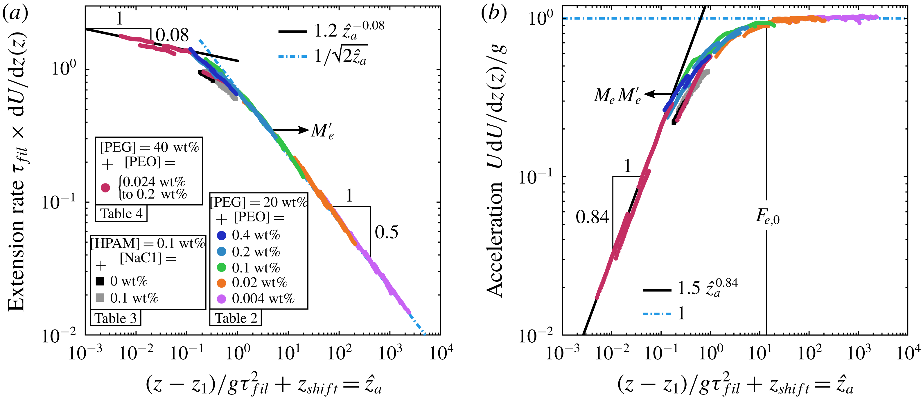
Regardless of the value of the initial velocity, in the inertial regime, again using (5.23) and (5.24), the dimensionless velocity field writes
 $$\begin{eqnarray}\hat{U} (\hat{z})=\sqrt{\hat{U} _{1}^{2}+2(\hat{z}-\hat{z}_{1}-s_{e})},\end{eqnarray}$$
where
 $s_{e}=s_{e,0}+\hat{U} _{1}^{2}/2-M_{e}^{-1}(\hat{U} _{1})$
. In the case of a negligible initial velocity
 $U_{1}\ll U_{e}$
, this regime is reached for
 $z\gg z_{e}$
. On the other hand, for initial velocities
 $U_{1}\gg U_{e}$
, inertia dominates over elastic forces even close to the slot and the flow is well approximated by a free fall
 $U^{2}=U_{1}^{2}+2g(z-z_{1})$
since
 $s_{e}$
goes to zero.
In figures 21(a) and 21(b), we present respectively the dimensionless extension rate
 $\dot{\unicode[STIX]{x1D716}}\unicode[STIX]{x1D70F}_{fil}$
where
 $\dot{\unicode[STIX]{x1D716}}=\text{d}U/\text{d}z$
and the dimensionless acceleration
 $[U\,\text{d}U/\text{d}z]/g$
as a function of
 $\hat{z}-\hat{z}_{1}+z_{shift}$
. The experimental data collapse on master curves which correspond to
 $M_{e}^{\prime }$
and
 $M_{e}M_{e}^{\prime }$
respectively, where
 $^{\prime }$
denotes spatial derivation
 $\text{d}/\text{d}\hat{z}$
. According to figure 21(a), the extension rate is of the order of
 $1/\unicode[STIX]{x1D70F}_{fil}$
in the elastic regime
 $z\ll z_{e}$
. More precisely,
 $\dot{\unicode[STIX]{x1D716}}\unicode[STIX]{x1D70F}_{fil}$
weakly decreases and is initially larger than the coil–stretch transition value
 $1/2$
. This result is reminiscent of the filament thinning experiment described in § 3.2 for which
 $\dot{\unicode[STIX]{x1D716}}\unicode[STIX]{x1D70F}_{fil}=2/3$
in the elastic regime. Physically, polymer chains are therefore expected to unravel in the elastic regime since
 $\unicode[STIX]{x1D70F}_{fil}\dot{\unicode[STIX]{x1D716}}=O(1)$
, and to return progressively to a coil state in the inertial regime where
 $\unicode[STIX]{x1D70F}_{fil}\dot{\unicode[STIX]{x1D716}}\ll 1$
.
We can now give a physical argument for the absence of finite extensibility effects in the curtain flow. First we need to estimate the total Hencky strain
 $\unicode[STIX]{x1D716}_{e}$
accumulated by the polymer chains in the elastic regime. We use the following high estimation
 $$\begin{eqnarray}\unicode[STIX]{x1D716}_{e}-\unicode[STIX]{x1D716}_{1}\approx \int _{t(z_{1})}^{t(z_{e})}\dot{\unicode[STIX]{x1D716}}\,\text{d}t=\int _{z_{1}}^{z_{e}}\,\text{d}U/U=\ln [U(z_{e})/U_{1}].\end{eqnarray}$$
We assume that the Hencky strain after swelling
 $\unicode[STIX]{x1D716}_{1}$
is less than
 $\unicode[STIX]{x1D716}_{e}$
since polymer chains are expected to unravel more in the curtain extensional flow than in the slot shear flow. Using (5.25) and taking
 $\unicode[STIX]{x1D6FC}=1$
for simplicity, i.e.
 $U(z)\approx U_{1}+K(z-z_{1})/\unicode[STIX]{x1D70F}_{fil}$
, we find
 $U(z_{e})\approx U_{1}+KU_{e}$
assuming
 $z_{1}\ll z_{e}$
. Finally, we get
 $\unicode[STIX]{x1D716}_{e}\approx \ln (1+K/\hat{U} _{1})$
. This value has to be compared to the critical Hencky strain
 $\unicode[STIX]{x1D716}^{\ast }$
above which the polymer deformation saturates to its maximum value. It can be estimated from CaBER data shown in figure 6. We get
 $\unicode[STIX]{x1D716}^{\ast }\approx 6$
for PEO and salted HPAM solutions and
 $\unicode[STIX]{x1D716}^{\ast }\approx 4$
for unsalted HPAM solutions. The condition for no finite extensibility effect writes
 $\unicode[STIX]{x1D716}_{e}\ll \unicode[STIX]{x1D716}^{\ast }$
, i.e. polymer chains must not reach their maximum length during the elastic regime. After injecting the estimation of
 $\unicode[STIX]{x1D716}_{e}$
, the condition becomes
 $\hat{U} _{1}\gg K/(\exp (\unicode[STIX]{x1D716}^{\ast })-1)$
which is
 $2\times 10^{-3}$
for PEO and salted HPAM solutions and
 $2\times 10^{-2}$
for unsalted HPAM solutions. This condition is fulfilled in most experiments (see values of
 $\hat{U} _{1}$
in figure 20
b) and the finite extensibility parameter
 $b$
does therefore not play a major role.
We now propose a simple model for the elastic regime exponent
 $\unicode[STIX]{x1D6FC}$
. Since polymer chains are highly stretched in the elastic regime, one can expect that the extensional viscosity scales as
 $\unicode[STIX]{x1D702}_{e}\propto \dot{\unicode[STIX]{x1D716}}^{m}$
with
 $m\gg 1$
, assuming that we are at the vicinity of the coil–stretch transition, as predicted by the FENE models (Herrchen & Öttinger Reference Herrchen and Öttinger1997; Larson Reference Larson1999). Taking an approach similar to the Newtonian case, we inject
 $U\propto z^{\unicode[STIX]{x1D6FC}}$
in the force balance equation (5.16) where we neglect inertia and take
 $\unicode[STIX]{x1D6E5}=\unicode[STIX]{x1D702}_{e}\dot{\unicode[STIX]{x1D716}}\propto (\text{d}U/\text{d}z)^{m+1}\propto z^{(\unicode[STIX]{x1D6FC}-1)(m+1)}$
. We get that
 $\unicode[STIX]{x1D6FC}=1+1/(m+1)$
is the only possible solution, which approaches
 $\unicode[STIX]{x1D6FC}=1$
for
 $m\gg 1$
. This is close to the experimental value
 $\unicode[STIX]{x1D6FC}=0.92$
. However, since the transient extensional viscosity
 $\unicode[STIX]{x1D702}_{e}(\dot{\unicode[STIX]{x1D716}},\unicode[STIX]{x1D716})$
, which is actually a function of both the local extension rate and the total strain accumulated by the polymer molecules, has no reason to reach the steady value anywhere in the elastic regime (i.e. where
 $t\ll \unicode[STIX]{x1D70F}_{fil}$
, which is equivalent to
 $z\ll z_{e}=g\unicode[STIX]{x1D70F}_{fil}^{2}$
), a better treatment of the problem lies in the use of a full constitutive equation. This is left for a future work.
Finally, we can derive an expression of the length
 $z_{e}^{\ast }$
of the sub-gravitational part of the curtain introduced in § 5.1. Let us define this length as
 $U\,\text{d}U/\text{d}z(z=z_{e}^{\ast })=0.95g$
where 0.95 is an arbitrary value close to 1 and let
 $F_{e,0}$
be such that
 $M_{e}M_{e}^{\prime }(\hat{z}=F_{e,0})=0.95$
. We obtain
 $F_{e,0}=12\pm 5$
(figure 21
b). Therefore, according to (5.24), we have
 $$\begin{eqnarray}z_{e}^{\ast }=F_{e}z_{e},\quad F_{e}=F_{e,0}+\hat{z}_{1}-M_{e}^{-1}(\hat{U} _{1}),\end{eqnarray}$$
where the prefactor
 $F_{e}$
is a decreasing function of the initial velocity.
5.5 Inelastic viscous curtains versus low viscosity elastic curtains
In the previous sections, we have characterised the curtain flow of both Newtonian and viscoelastic liquids. In particular, the lengths of the sub-gravitational parts of the curtains are given respectively by
 $z_{v}$
and
 $z_{e}$
(5.2) and (5.21) with prefactors which are decreasing functions of the initial velocity. For a given viscoelastic liquid with zero-shear viscosity
 $\unicode[STIX]{x1D702}_{0}$
, density
 $\unicode[STIX]{x1D70C}$
and extensional relaxation time
 $\unicode[STIX]{x1D70F}_{fil}$
, we define a dimensionless number
 $$\begin{eqnarray}\mathit{El}=\left(\frac{z_{e}}{z_{v}}\right)^{1/2}=\frac{\unicode[STIX]{x1D70F}_{fil}g^{2/3}}{(4\unicode[STIX]{x1D702}_{0}/\unicode[STIX]{x1D70C})^{1/3}}\end{eqnarray}$$
which measures the relative importance of elastic to viscous effects in the curtain flow. The general definition of the elasticity number is
 $\mathit{El}=\mathit{Wi}/Re=\unicode[STIX]{x1D70F}_{fil}\unicode[STIX]{x1D702}/(\unicode[STIX]{x1D70C}L^{2})$
where
 $\mathit{Wi}=\unicode[STIX]{x1D70F}_{fil}U/L$
and
 $Re=\unicode[STIX]{x1D70C}UL/\unicode[STIX]{x1D702}$
are respectively the Weissenberg and Reynolds numbers and
 $U$
and
 $L$
are characteristic velocity and length scales of the flow. Hence,
 $(z_{e}/z_{v})^{1/2}$
is an elasticity number based on the viscous length
 $L=z_{v}$
. Values of
 $\mathit{El}$
are reported in tables 2–4. As expected, it is larger than one since
 $z_{e}\gg z_{v}$
in our experiments, except for solutions with low polymer concentrations exhibiting a free fall, for which both
 $z_{e}$
and
 $z_{v}$
are less than a few millimetres. Therefore, elasticity dominates over viscosity in our experiments. However, when adding polymer molecules to a viscous Newtonian solvent with a large value of
 $z_{v}$
, we can expect a transition from the viscous regime described in § 5.2 with exponent 2 (5.10) to the elastic regime described in § 5.4 with exponent
 $\unicode[STIX]{x1D6FC}=0.92$
(5.25) when
 $\mathit{El}$
becomes larger than one.
6 Elastic stress at the slot exit
In this section, we address the question of the origin of the elastic stress in the curtain. In the previous section, we have assumed that it comes mostly from the extensional stretching of polymer molecules in the curtain, especially in the elastic regime where
 $\unicode[STIX]{x1D70F}_{fil}\dot{\unicode[STIX]{x1D716}}=O(1)$
. However, one other possible origin lies is the initial shear deformation (or ‘pre-shear’) of polymer molecules in the slot, which may lead to unrelaxed stress on top of the curtain. We start this discussion by investigating the die swell ratio.
6.1 The die swell ratio
The liquid swells at the slot exit due to the recovery of the elastic strain imparted into the die. In the theory of Tanner (Reference Tanner1970, Reference Tanner2005), and Huang & White (Reference Huang and White1979), the swelling ratio is
 $$\begin{eqnarray}\unicode[STIX]{x1D709}=\frac{U_{s}}{U_{1}}=\left[1+\frac{3-m}{m+1}\left(\frac{N_{1}}{2\unicode[STIX]{x1D70E}}\right)_{w}^{2}\right]^{1/4},\end{eqnarray}$$
where
 $N_{1}=\unicode[STIX]{x1D70E}_{zz}^{\ast }-\unicode[STIX]{x1D70E}_{yy}^{\ast }$
and
 $\unicode[STIX]{x1D70E}=\unicode[STIX]{x1D70E}_{yz}^{\ast }$
are respectively the normal stress difference and the shear stress,
 $m$
is such that
 $N_{1}\propto \unicode[STIX]{x1D70E}^{m}$
, and subscript
 $_{w}$
indicates that
 $N_{1}$
and
 $\unicode[STIX]{x1D70E}$
are to be taken at the wall of the slot, i.e. at
 $y=a$
. Note that
 $\unicode[STIX]{x1D748}^{\ast }$
is the local stress tensor. This formula, which was developed for melts, has also been used in the context of polymer solutions (Allain, Cloitre & Perrot Reference Allain, Cloitre and Perrot1997). Let us compare the experimental data presented in figure 15 for the PEO solution of table 5 with Tanner’s prediction (6.1). Since the wall shear rate
 $\dot{\unicode[STIX]{x1D6FE}}_{w}\sim U_{s}/a$
is larger than the shear rate
 $\dot{\unicode[STIX]{x1D6FE}}_{c}=3~\text{s}^{-1}$
at which shear thinning starts, the Carreau law (3.1) can be reduced to an Ostwald power law
 $\unicode[STIX]{x1D70E}=K_{0}\dot{\unicode[STIX]{x1D6FE}}^{n}$
with
 $K_{0}=\unicode[STIX]{x1D702}_{0}/\dot{\unicode[STIX]{x1D6FE}}_{c}^{n-1}$
and the wall shear rate can be simplified to
 $$\begin{eqnarray}\dot{\unicode[STIX]{x1D6FE}}_{w}=\frac{2n+1}{n}\frac{U_{s}}{a},\end{eqnarray}$$
which ranges between 290 and
 $900~\text{s}^{-1}$
. We can therefore use the parameters of table 5 since shear rheology measurements are performed for shear rates up to
 $500~\text{s}^{-1}$
for this liquid, which is close to
 $\dot{\unicode[STIX]{x1D6FE}}_{w}$
.
Comparison between the experimental die swell ratio
 $\unicode[STIX]{x1D709}=U_{s}/U_{1}$
for the data of figure 15 and the values predicted by Tanner’s unconstrained recovery theory (6.1) where we use
 $(N_{1})_{w}=N_{1}(\dot{\unicode[STIX]{x1D6FE}}_{w})=\unicode[STIX]{x1D6F9}\dot{\unicode[STIX]{x1D6FE}}_{w}^{\unicode[STIX]{x1D6FC}_{1}}$
and
 $(\unicode[STIX]{x1D70E})_{w}=\unicode[STIX]{x1D70E}(\dot{\unicode[STIX]{x1D6FE}}_{w})=K_{0}\dot{\unicode[STIX]{x1D6FE}}_{w}^{n}$
where
 $\dot{\unicode[STIX]{x1D6FE}}_{w}$
is the wall shear rate (6.2). Since
 $N_{1}\propto \unicode[STIX]{x1D70E}^{m}$
, we use
 $m=\unicode[STIX]{x1D6FC}_{1}/n$
.

The experimental die swell ratio
 $\unicode[STIX]{x1D709}$
is shown in figure 22 along with the predictions of (6.1) and (6.2). The theory clearly overpredicts the die swell ratio. This is not surprising since the unconstrained recovery theory of Tanner is only valid if the extruded sheet is load free, i.e. in the absence of tensile stress. A correction has been proposed in the context of fibre spinning (White & Roman Reference White and Roman1976) (which is equivalent to film casting) but not in the context of free jets or curtains subjected to gravity only. The die swell ratio is generally assumed to be only slightly modified by gravity for free jets (Richardson Reference Richardson1970). However, in the planar case, Huang & White (Reference Huang and White1979) report significant discrepancies between Tanner’s theory and their experimental results when extruding melts from slit dies into ambient air, like in figure 22. They report that Tanner’s law was recovered when extruding into a bath of silicone oil with the same density, in which case the curtain no longer necks down after swelling due to gravity (i.e.
 $h$
and
 $U$
are constant). In the latter case, according to the force balance equation (5.16) without inertia,
 $\unicode[STIX]{x1D6E5}$
must therefore be constant. In the theory of Tanner, it is assumed that most fluid particles ‘rapidly’ switch from the state of fully developed flow in the slot to a state of zero stress measured relative to atmospheric pressure as datum. Here, ‘rapidly’ means that the time needed to clear the exit zone is short compared to the polymer relaxation time, i.e.
 $U_{s}\unicode[STIX]{x1D70F}_{fil}/a\gg 1$
which is the case in figure 22. In other words, the mean normal stress difference
 $\unicode[STIX]{x1D6E5}$
defined in § 5.3 by
 $$\begin{eqnarray}\unicode[STIX]{x1D6E5}=\frac{1}{h}\int _{0}^{h}(\unicode[STIX]{x1D70E}_{zz}^{\ast }-\unicode[STIX]{x1D70E}_{yy}^{\ast })\,\text{d}y,\end{eqnarray}$$
switches from a value
 $\unicode[STIX]{x1D6E5}_{s}$
inside the slot to a value
 $\unicode[STIX]{x1D6E5}_{1}=\unicode[STIX]{x1D6E5}(z_{1})$
after swelling (figure 16) which is
 $\unicode[STIX]{x1D6E5}_{1}=0$
in the absence of gravity. The discrepancy in figure 22 suggests that
 $\unicode[STIX]{x1D6E5}_{1}\neq 0$
in the presence of an axial tension due to gravity.
These results suggest that the elastic stress imparted into the die may have an effect on the curtain flow downstream. In order to quantify this effect, we now compare the value of the mean normal stress difference
 $\unicode[STIX]{x1D6E5}_{s}$
inside the die and
 $\unicode[STIX]{x1D6E5}_{1}$
after swelling.
6.2 Mean normal stress difference before and after swelling
We find
 $\unicode[STIX]{x1D6E5}_{s}$
can be estimated analytically. We consider a shear-thinning fluid following an Ostwald power law
 $\unicode[STIX]{x1D70E}=K_{0}\dot{\unicode[STIX]{x1D6FE}}^{n}$
for simplicity. Assuming a fully developed Poiseuille flow, the local velocity inside the slot is
 $$\begin{eqnarray}u(y)=U_{s}\frac{2n+1}{n+1}(1-(|y|/a)^{1+1/n}).\end{eqnarray}$$
Using
 $N_{1}=\unicode[STIX]{x1D6F9}\dot{\unicode[STIX]{x1D6FE}}^{\unicode[STIX]{x1D6FC}_{1}}$
and
 $\dot{\unicode[STIX]{x1D6FE}}=\text{d}u/\text{d}y$
, we find
 $$\begin{eqnarray}\unicode[STIX]{x1D6E5}_{s}=\frac{1}{a}\int _{0}^{a}N_{1}\,\text{d}y=\frac{n}{\unicode[STIX]{x1D6FC}_{1}+n}\left(\frac{2n+1}{n}\right)^{\unicode[STIX]{x1D6FC}_{1}}\unicode[STIX]{x1D6F9}\left(\frac{U_{s}}{a}\right)^{\unicode[STIX]{x1D6FC}_{1}}.\end{eqnarray}$$
Now we show how to obtain the value of the mean normal stress difference
 $\unicode[STIX]{x1D6E5}_{1}$
after swelling based on the Lagrangian force balance equation derived in § 5.3. We can reasonably assume that
 $\unicode[STIX]{x1D6E5}$
becomes negligible in the asymptotic free-fall regime where the extension rate goes to 0 (figure 21
a). Hence, according to (5.20) (where we choose to start from
 $z_{1}\approx 2.5~\text{mm}$
), the curtain velocity
 $U$
reaches an oblique asymptote of equation
 $$\begin{eqnarray}(U-U_{1})/g\unicode[STIX]{x1D70F}_{fil}=(t-t_{1})/\unicode[STIX]{x1D70F}_{fil}-A_{e},\end{eqnarray}$$
where
 $$\begin{eqnarray}A_{e}=\unicode[STIX]{x1D6E5}_{1}/\unicode[STIX]{x1D70C}gU_{1}\unicode[STIX]{x1D70F}_{fil}=\unicode[STIX]{x1D6E5}_{1}/\unicode[STIX]{x1D70C}U_{1}U_{e}=\hat{\unicode[STIX]{x1D6E5}}_{1}/\hat{U} _{1},\end{eqnarray}$$
where
 $\hat{\unicode[STIX]{x1D6E5}}_{1}=\unicode[STIX]{x1D6E5}_{1}/\unicode[STIX]{x1D6E5}_{e}$
and
 $\unicode[STIX]{x1D6E5}_{e}=\unicode[STIX]{x1D70C}gz_{e}=\unicode[STIX]{x1D70C}U_{e}^{2}=\unicode[STIX]{x1D70C}(g\unicode[STIX]{x1D70F}_{fil})^{2}$
which is the natural scaling for
 $\unicode[STIX]{x1D6E5}$
in the force balance equation (5.16) for a low viscosity elastic liquid. To estimate
 $A_{e}$
, we plot
 $(U-U_{1})/g\unicode[STIX]{x1D70F}_{fil}$
as a function of
 $(t-t_{1})/\unicode[STIX]{x1D70F}_{fil}$
, as shown in figure 23(a) for some liquids with extensional relaxation times
 $\unicode[STIX]{x1D70F}_{fil}$
ranging between 0.008 s and 0.68 s. Since we could not always observe the asymptotic free-fall regime, we use the master curve
 $M_{e}$
identified in figure 20(a) to extend the experimental data and we fit the free-fall regime by an oblique asymptote to obtain the value of
 $A_{e}$
(figure 23
a). In order to validate this method, we performed an additional experiment where a long curtain is observed at various vertical positions to obtain a more complete velocity field
 $U(z)$
for
 $\unicode[STIX]{x1D70F}_{fil}=0.1~\text{s}$
. Unfortunately, the curtain spontaneously breaks at
 $z\approx 100~\text{cm}$
due to the shear instability mentioned in § 4.3 and we can still not observe the free-fall regime since
 $z_{e}^{\ast }\approx 120~\text{cm}$
. However, the flow for
 $z\leqslant 100~\text{cm}$
fits perfectly onto the master curve
 $M_{e}$
, and the data presented in figure 23(a) are comparable to the data corresponding to almost the same liquid observed for
 $z\leqslant 20~\text{cm}$
, which validates the method presented here to estimate
 $A_{e}$
.
(a)
 $(U-U_{1})/g\unicode[STIX]{x1D70F}_{fil}$
versus
 $(t-t_{1})/\unicode[STIX]{x1D70F}_{fil}$
, where subscript
 $_{1}$
refers to the altitude
 $z_{1}\approx 2.5~\text{mm}$
and
 $t$
is the Lagrangian time (5.17), for five liquids. Liquid 1: degraded (
 $t_{d}=100~\text{min}$
) 0.02 wt% PEO solution with 20 wt% PEG solvent (table 2), liquid 2: degraded (
 $t_{d}=60~\text{min}$
) 0.1 wt% PEO solution with 20 wt% PEG solvent (table 2), liquid 3: degraded (
 $t_{d}=100~\text{min}$
) 0.4 wt% PEO solution with 20 wt% PEG solvent (table 2), liquid 4: 0.11 wt% PEO solution with 40 wt% PEG solvent (table 4). The curtain length
 $L_{c}$
is 30 cm for liquids 1, 2 and 3 and is 200 cm for liquid 4. Liquid 5: liquid close to liquid 3 for
 $L_{c}=100~\text{cm}$
and observed at various vertical positions to obtain a more complete velocity field
 $U(z)$
. The experimental data are extended with the master curve
 $M_{e}$
(figure 20) and the free-fall regime is fitted by (6.6). (b) Values of
 $A_{e}$
versus
 $U_{1}/U_{e}=U_{1}/g\unicode[STIX]{x1D70F}_{fil}$
for some of the liquids of figure 20.

Values of
 $A_{e}$
are presented in figure 23(b) for various solutions as a function of the dimensionless initial velocity
 $\hat{U} _{1}=U_{1}/U_{e}$
. For
 $\hat{U} _{1}\leqslant 1$
, the experimental data are well captured by
 $$\begin{eqnarray}A_{e}\approx 1.4\hat{U} _{1}^{-0.2},\end{eqnarray}$$
which, according to (6.7), gives finally
 $$\begin{eqnarray}\unicode[STIX]{x1D6E5}_{1}\approx 1.4\unicode[STIX]{x1D70C}g^{1.2}U_{1}^{0.8}\unicode[STIX]{x1D70F}_{fil}^{1.2}.\end{eqnarray}$$
A different behaviour is observed for
 $\hat{U} _{1}\geqslant 1$
. The slope switches from
 $-0.2$
to approximately
 $-2$
.
As we now show, this result is analogous to Newtonian curtains. Since die swell can be neglected (Tanner Reference Tanner2000), the mean normal stress difference instantaneously switches from
 $\unicode[STIX]{x1D6E5}_{s}=0$
inside the slot to a value
 $\unicode[STIX]{x1D6E5}_{0}=\unicode[STIX]{x1D6E5}(z=0)=4\unicode[STIX]{x1D702}\,\text{d}U/\text{d}z(z=0)$
at the slot exit. In dimensionless form, we obtain
 $\bar{\unicode[STIX]{x1D6E5}}_{0}=\bar{U}^{\prime }(\bar{z}=0)$
where
 $\bar{\unicode[STIX]{x1D6E5}}=\unicode[STIX]{x1D6E5}/\unicode[STIX]{x1D6E5}_{v}$
and
 $\unicode[STIX]{x1D6E5}_{v}=\unicode[STIX]{x1D70C}gz_{v}=\unicode[STIX]{x1D70C}U_{v}^{2}=\unicode[STIX]{x1D70C}(4\unicode[STIX]{x1D702}g/\unicode[STIX]{x1D70C})^{2/3}$
which is the natural scaling for
 $\unicode[STIX]{x1D6E5}$
in the force balance equation (5.16) for a viscous Newtonian liquid. Equation (5.10) gives
 $\bar{\unicode[STIX]{x1D6E5}}_{0}=(2\bar{U}_{0})^{1/2}$
for
 $\bar{U}_{0}\ll 1$
, i.e.
 $\unicode[STIX]{x1D6E5}_{0}=2\sqrt{2}\unicode[STIX]{x1D70C}(gU_{0}\unicode[STIX]{x1D702}/\unicode[STIX]{x1D70C})^{0.5}$
. We can also define
 $A_{v}=\unicode[STIX]{x1D6E5}_{0}/\unicode[STIX]{x1D70C}U_{0}U_{v}=\bar{\unicode[STIX]{x1D6E5}}_{0}/\bar{U}_{0}$
, and we obtain
 $A_{v}=\sqrt{2}\bar{U}_{0}^{-1/2}$
for
 $\bar{U}_{0}\ll 1$
where the exponent
 $-0.5$
is larger (in absolute value) than the exponent
 $-0.2$
found in the viscoelastic case. Note that for
 $\bar{U}_{0}\gg 1$
, in which case the curtain flow is a free fall even close to the slot, we have
 $\bar{\unicode[STIX]{x1D6E5}}_{0}=1/\bar{U}_{0}$
and
 $A_{v}=\bar{U}_{0}^{-2}$
, which is analogous to the
 $\hat{U} _{1}\geqslant 1$
part of the curve of figure 23(b).
In order to get more information about the physical meaning of
 $\unicode[STIX]{x1D6E5}_{1}$
, we can use the integrated force balance equation (5.19) which we write here in its Eulerian form for more clarity
 $$\begin{eqnarray}2h_{1}\unicode[STIX]{x1D6E5}_{1}-2h\unicode[STIX]{x1D6E5}=\unicode[STIX]{x1D70C}q(U_{1}-U)+2\unicode[STIX]{x1D70C}g\int _{z_{1}}^{z}h(z^{\ast })\,\text{d}z^{\ast },\end{eqnarray}$$
where
 $2h_{1}=2h(z_{1})=q/U_{1}$
. In the elastic regime
 $z\ll z_{e}$
, the inertia term is negligible and the weight of the curtain between
 $z_{1}$
and
 $z$
is supported by the difference between the contact forces
 $2h_{1}\unicode[STIX]{x1D6E5}_{1}$
and
 $2h\unicode[STIX]{x1D6E5}$
acting respectively on the upper and lower side. This shows that
 $\unicode[STIX]{x1D6E5}_{1}$
is the mean normal stress difference which is necessary to bear the weight of the sub-gravitational part of the curtain. We can derive the previous results by neglecting inertia and returning to the Lagrangian description. We obtain in the elastic regime
 $t\ll \unicode[STIX]{x1D70F}_{fil}$
 $$\begin{eqnarray}\unicode[STIX]{x1D6E5}_{1}/U_{1}-\unicode[STIX]{x1D6E5}/U\approx \unicode[STIX]{x1D70C}g(t-t_{1}).\end{eqnarray}$$
Assuming that
 $\unicode[STIX]{x1D6E5}$
becomes negligible at the transition to free fall (
 $t\approx \unicode[STIX]{x1D70F}_{fil}$
) and that
 $t_{1}\ll \unicode[STIX]{x1D70F}_{fil}$
, we find that
 $\unicode[STIX]{x1D6E5}_{1}\propto \unicode[STIX]{x1D70C}gU_{1}\unicode[STIX]{x1D70F}_{fil}$
with a prefactor
 $A_{e}$
which must be a decreasing function of the dimensionless initial velocity
 $\hat{U} _{1}$
since the length of the sub-gravitational part of the curtain is
 $z_{e}^{\ast }=F_{e}z_{e}$
where
 $F_{e}$
is a decreasing function of
 $\hat{U} _{1}$
. In particular, as expected from the discussion about Tanner’s theory,
 $\unicode[STIX]{x1D6E5}_{1}=0$
in the absence of gravity.
For the experiments presented so far, using (6.5) and (6.7), we obtain
 $$\begin{eqnarray}\frac{\unicode[STIX]{x1D6E5}_{1}}{\unicode[STIX]{x1D6E5}_{s}}=\left[\frac{n}{\unicode[STIX]{x1D6FC}_{1}+n}\left(\frac{2n+1}{n}\right)^{\unicode[STIX]{x1D6FC}_{1}}\right]^{-1}\frac{A_{e}\unicode[STIX]{x1D70C}g\unicode[STIX]{x1D70F}_{fil}U_{1}}{\unicode[STIX]{x1D6F9}(U_{s}/a)^{\unicode[STIX]{x1D6FC}_{1}}}.\end{eqnarray}$$
Estimating
 $A_{e}$
by the method presented in this section, we find
 $\unicode[STIX]{x1D6E5}_{1}/\unicode[STIX]{x1D6E5}_{s}=O(1)$
. More precisely, it decreases from 2.5 to 0.5 for the liquid of table 5 used in figures 15 and 22 when increasing the flow rate, and it is equal to
 $0.6\pm 0.1$
for all PEO solutions with 40 wt% PEG solvent of table 4. In the latter case, the elastic stress rapidly decreases when leaving the slot as the polymer chains undergo a rapid strain
 $\unicode[STIX]{x1D716}=\ln (U_{1}/U_{s})=-\ln (\unicode[STIX]{x1D709})<0$
during swelling. However, in the presence of gravity, the sheet is not load free and the swelling ratio is less than expected since some elastic stress
 $\unicode[STIX]{x1D6E5}_{1}\neq 0$
has to bear the weight of the sub-gravitational part of the curtain. In other words, the polymer chains cannot recover their equilibrium shape after swelling.
A question which remains unanswered is the link between
 $\unicode[STIX]{x1D6E5}_{1}$
and
 $\unicode[STIX]{x1D6E5}_{s}$
. Since the experiments presented so far indicate that
 $\unicode[STIX]{x1D6E5}_{1}/\unicode[STIX]{x1D6E5}_{s}=O(1)$
, one might think that
 $\unicode[STIX]{x1D6E5}_{1}$
is intrinsically linked to
 $\unicode[STIX]{x1D6E5}_{s}$
. If so, the origin of the polymeric stress would lie in the shear deformation of the polymer chains in the slot, in which case the length
 $z_{e}^{\ast }$
of the sub-gravitational regime would be a function of
 $\unicode[STIX]{x1D6E5}_{s}$
. In particular, a curtain of vanishing slot velocity
 $U_{s}$
would exhibit no sub-gravitational elastic regime (although
 $U_{1}\ll g\unicode[STIX]{x1D70F}_{fil}$
) since
 $\unicode[STIX]{x1D6E5}_{s}$
, and therefore
 $\unicode[STIX]{x1D6E5}_{1}$
, would be arbitrarily small. However the fact that we find
 $\unicode[STIX]{x1D6E5}_{1}/\unicode[STIX]{x1D6E5}_{s}=O(1)$
might also be a coincidence. To answer this question, we need to compare the flow of two curtains made of the same liquid but with radically different values of
 $\unicode[STIX]{x1D6E5}_{s}$
. According to (6.5) and (6.9), changing the slot thickness
 $2a$
while keeping the same initial velocity
 $U_{1}$
is a good solution: if
 $\unicode[STIX]{x1D6E5}_{1}$
does not change while
 $\unicode[STIX]{x1D6E5}_{s}$
changes, it means that the origin of the polymeric stress lies in the extensional deformation of polymer molecules once in the free-surface curtain. If so, the description of the flow provided in § 5.4 is universal and the master curve
 $M_{e}$
does not depend on the pre-shear history upstream of the curtain.
6.3 The influence of the die geometry
In order to check if
 $\unicode[STIX]{x1D6E5}_{1}$
is intrinsically linked to
 $\unicode[STIX]{x1D6E5}_{s}$
or not, i.e. whether or not the curtain flow is affected by the history of polymer deformations upstream of the curtain, we compare the flow of two curtains of same length made of the same liquid (table 5) and extruded from different dies. The first curtain is extruded from the slot die of figure 1(b) where the slot thickness is
 $2a=1~\text{mm}$
. The flow rate is
 $q=1.4~\text{cm}^{2}~\text{s}^{-1}$
, the mean velocity is
 $U_{s}=q/2a=0.14~\text{m}~\text{s}^{-1}$
in the slot and
 $U_{1}=0.085~\text{m}~\text{s}^{-1}$
at
 $z_{1}=2.5~\text{mm}$
from the slot exit, after an initial swelling of ratio
 $\unicode[STIX]{x1D709}=U_{s}/U_{1}=1.6>1$
. The second curtain is formed using a second ‘die’ presented in figure 24(a) where the liquid flows freely along an inclined plane before forming a vertical curtain when falling off the edge. Imposing a flow rate
 $q^{\star }=0.85~\text{cm}^{2}~\text{s}^{-1}<q$
, we measure that the thickness of the liquid layer flowing down the plane is
 $2a^{\star }=2.5~\text{mm}>2a$
, which gives a mean velocity
 $U_{s}^{\star }=q^{\star }/2a^{\star }=0.034~\text{m}~\text{s}^{-1}<U_{s}$
. We measure that the mean vertical velocity is
 $U_{1}^{\star }=0.088~\text{m}~\text{s}^{-1}\approx U_{1}$
at 3 mm from the edge of the plane. Therefore, the thickness of the liquid rapidly decreases by a factor
 $\unicode[STIX]{x1D709}^{\star }=U_{s}^{\star }/U_{1}^{\star }=0.39<1$
at the edge of the plane.
(a) Sketch of a curtain formed when a liquid layer of thickness
 $2a^{\star }$
falls off the edge of an inclined plane with mass flow
 $Q$
. A grid of straws is used to homogenise the flow in the
 $x$
direction and the linear flow rate is
 $q=Q/\unicode[STIX]{x1D70C}l$
where
 $l$
is the curtain width. Guides are used to avoid sheet retraction. (b) Using the PEO solution of table 5, comparison of the squared velocity field
 $U^{2}(z)$
of the curtain formed using the inclined plane and using the slot die of figure 1(b). Both curtains start with comparable initial velocities
 $U_{1}$
and share the same length
 $L_{c}=50~\text{cm}$
. The typical shear rate is
 $U_{s}/a=280~\text{s}^{-1}$
in the slot but is only
 $U_{s}^{\star }/2a^{\star }=14~\text{s}^{-1}$
along the inclined plane, i.e. 20 times less.
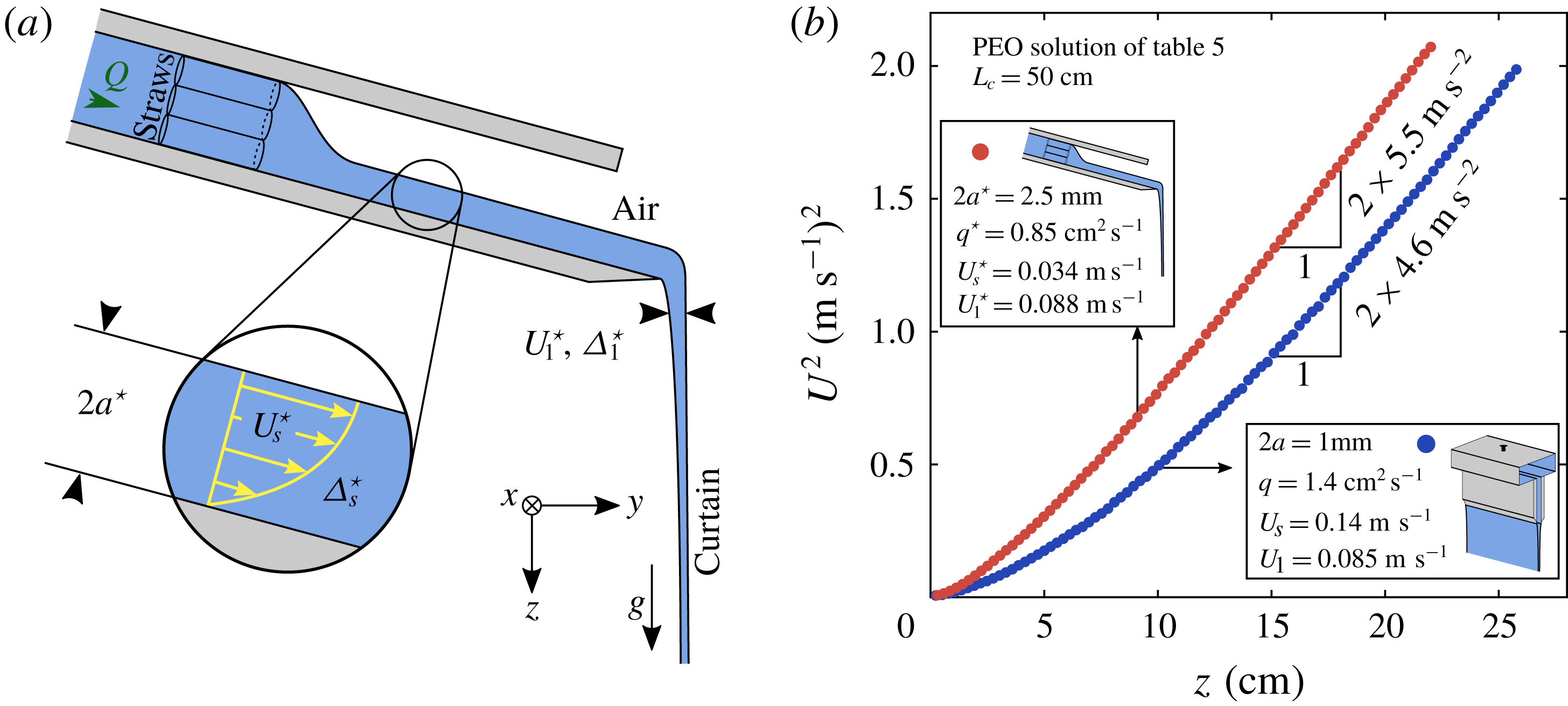
As presented in figure 24(b), the flows of these two curtains are slightly different. The liquid velocity, which is initially comparable since
 $U_{1}^{\star }\approx U_{1}$
, increases a bit faster when falling off the edge of the plane than when being extruded from the slot. Therefore, the flow of the curtain falling of the inclined plane does not perfectly collapse on the master curve
 $M_{e}$
identified in figure 20(a). Let us estimate
 $\unicode[STIX]{x1D6E5}_{s}$
and
 $\unicode[STIX]{x1D6E5}_{1}$
for these two curtains.
We find
 $\unicode[STIX]{x1D6E5}_{s}\approx 690~\text{Pa}$
for the slot die. For the inclined plane, we estimate the mean normal stress difference
 $\unicode[STIX]{x1D6E5}_{s}^{\star }$
developed by the liquid when flowing down the plane using (6.5) where
 $a$
is replaced by
 $2a^{\star }$
since the flow is a semi-Poiseuille. We find
 $\unicode[STIX]{x1D6E5}_{s}^{\star }\approx 1.6~\text{Pa}$
which is much less than
 $\unicode[STIX]{x1D6E5}_{s}$
. Hence, this change in die geometry reduces the elastic stress upstream of the curtain by a factor
 $\unicode[STIX]{x1D6E5}_{s}^{\star }/\unicode[STIX]{x1D6E5}_{s}\approx 2\times 10^{-3}\ll 1$
. Hence, the effect of
 $\unicode[STIX]{x1D6E5}_{s}$
on the curtain flow identified in figure 24(b) is actually very weak. Indeed, despite a much different flow upstream of the curtain, the curtain flows are quite comparable. Therefore, the mean normal stress difference
 $\unicode[STIX]{x1D6E5}_{1}$
developed a few millimetres below slot or below the edge of the plane respectively must be comparable in both experiments. Using the method described in § 6.2, we find
 $A_{e}\approx 3.4$
for the slot die and
 $A_{e}^{\star }\approx 2.1$
for the inclined plane. In the latter case, note that this estimation is based on comparisons with other curtain flows from the slot die since the master curve can not be used to extend the experimental data. We find respectively
 $\unicode[STIX]{x1D6E5}_{1}\approx 460~\text{Pa}$
and
 $\unicode[STIX]{x1D6E5}_{1}^{\star }\approx 300~\text{Pa}$
which are indeed comparable, i.e.
 $\unicode[STIX]{x1D6E5}_{1}^{\star }/\unicode[STIX]{x1D6E5}_{1}\approx 0.6$
. For the slot die, the polymeric stress decreases during swelling and
 $\unicode[STIX]{x1D6E5}_{1}/\unicode[STIX]{x1D6E5}_{s}\approx 0.7<1$
. However, for the inclined plane, the polymeric stress increases during the contraction at the edge of the plane and
 $\unicode[STIX]{x1D6E5}_{1}^{\star }/\unicode[STIX]{x1D6E5}_{s}^{\star }\approx 180>1$
. In fact, in both cases, the polymer molecules undergo a rapid strain
 $\unicode[STIX]{x1D716}=\ln (U_{1}/U_{s})$
which is
 $-0.50<0$
for the slot and which is
 $0.95>0$
for the inclined plane. According to figure 6, such strains can indeed cause significant modifications of the polymeric stress.
To summarise, the mean normal stress difference switches from a value
 $\unicode[STIX]{x1D6E5}_{s}$
inside the die to a value
 $\unicode[STIX]{x1D6E5}_{1}$
at the die exit, where
 $\unicode[STIX]{x1D6E5}_{1}$
is of order
 $\unicode[STIX]{x1D70C}gU_{1}\unicode[STIX]{x1D70F}_{fil}$
independently of the flow history inside the die, with a prefactor
 $A_{e}$
which is a decreasing function of the initial velocity. However, since the flow is slightly modified when changing
 $\unicode[STIX]{x1D6E5}_{s}$
, the prefactor also depends on the die geometry and is an increasing function of
 $\unicode[STIX]{x1D6E5}_{s}$
. The length
 $z_{e}^{\ast }$
of the sub-gravitational regime is of order
 $g\unicode[STIX]{x1D70F}_{fil}^{2}$
with a prefactor
 $F_{e}$
which is a decreasing function of the initial velocity and which is also an increasing function of
 $\unicode[STIX]{x1D6E5}_{s}$
. In simple words, polymeric stresses in the curtain are mostly due to the extensional stretching of polymer molecules in the curtain (where
 $\unicode[STIX]{x1D70F}_{fil}\dot{\unicode[STIX]{x1D716}}=0(1)$
in the elastic regime), with a small correction due to the ‘pre-shear’ in the die.
7 Curtain stability
In this section, we investigate the influence of viscoelasticity on the stability of the curtain in terms of spontaneous hole opening events. The unstable curtain flows described in § 4.2 are not considered in this section.
7.1 Dynamics of hole opening
(a) Time evolution of a hole forming spontaneously in a curtain of 20 wt% PEG solvent with flow rate
 $q=3.3~\text{cm}^{2}~\text{s}^{-1}$
and length
 $L_{c}=30~\text{cm}$
. The hole is advected by the flow (self-healing). (b) Image superposition.

In figure 25(a,b), we show the time evolution of a hole forming spontaneously in a Newtonian curtain of 20 wt% PEG solvent. Such a hole can be initiated by impurities in the liquid such as bubbles which are inevitably generated in the hydraulic loop. The hole in figure 25 is advected by the flow while growing in size and the liquid is collected in a rim. According to Taylor (Reference Taylor1959) and Culick (Reference Culick1960), if capillary forces are only balanced by inertia, the local retraction speed of the hole in the reference frame of the moving liquid is
 $$\begin{eqnarray}V=\sqrt{\unicode[STIX]{x1D6FE}/\unicode[STIX]{x1D70C}h},\end{eqnarray}$$
where
 $\unicode[STIX]{x1D70C}$
and
 $\unicode[STIX]{x1D6FE}$
are the liquid density and surface tension and
 $h(z)$
is the local half-thickness of the curtain. In the case of a Newtonian liquid of dynamic viscosity
 $\unicode[STIX]{x1D702}$
, Savva & Bush (Reference Savva and Bush2009) showed that the retraction speed of the sheet when a hole initiated in a motionless sheet of constant thickness goes from 0 to
 $V$
in a time which increases as the Ohnesorge number
 $\mathit{Oh}=\unicode[STIX]{x1D702}/(4h\unicode[STIX]{x1D70C}\unicode[STIX]{x1D6FE})^{1/2}$
increases. Capillary forces are initially balanced by viscous forces before inertia finally dominates. Based on similar results, Sünderhauf, Raszillier & Durst (Reference Sünderhauf, Raszillier and Durst2002) concluded that increasing the liquid viscosity stabilises the curtain since the dynamics of hole opening is slowed down temporarily. Karim et al. (Reference Karim, Suszynski, Griffith, Pujari, Francis and Carvalho2018b
) recently measured the retraction speed of the sheet when a hole is initiated in curtains made of low viscosity PEO solutions. They report that the ratio of the local retraction speed to the local Taylor–Culick velocity decreases when the local Ohnesorge number increases for
 $\mathit{Oh}$
ranging between 0.22 and 0.43. This ratio was 0.95 for the solution with the highest extensional relaxation time
 $\unicode[STIX]{x1D70F}_{fil}=0.16~\text{s}$
and the authors conclude that elastic stresses slow down the hole opening process.
In the case where both viscous and elastic effects can be neglected, the part of the liquid rim corresponding to the upper edge of the hole retracts at velocity
 $V-U$
in the reference frame of the laboratory, where
 $V$
is calculated based on the local curtain thickness
 $2h(z)$
and where
 $U(z)$
is the local velocity of the surrounding liquid. This local competition can be written in terms of a Weber number
 $$\begin{eqnarray}\mathit{We}=\left(\frac{U}{V}\right)^{2}=\frac{\unicode[STIX]{x1D70C}hU^{2}}{\unicode[STIX]{x1D6FE}}=\frac{\unicode[STIX]{x1D70C}qU}{2\unicode[STIX]{x1D6FE}},\end{eqnarray}$$
which can be less than one close to the slot and become larger than one downstream. Therefore, if a hole opens at an altitude where
 $\mathit{We}>1$
, i.e. where advection is faster than the hole opening process, it will be carried away by the flow, as in figure 25. This process is often referred to as self-healing. However, if a hole opens in the unstable part of the curtain where
 $\mathit{We}<1$
, the upper edge of the hole propagates upwards and stops when reaching the slot whereas the lower end propagates downwards, in which case the curtain is finally split into two parts delimited by a rim which takes the form of an arch. The latter scenario is not possible if the Weber number is larger than one everywhere, i.e. if the initial velocity
 $U_{s}=q/2a$
at the slot exit is larger than the value of
 $V$
at the slot exit. Equivalently, the linear flow rate
 $q$
has to be larger than a critical value
 $$\begin{eqnarray}q_{\unicode[STIX]{x1D6FE}}=(4a\unicode[STIX]{x1D6FE}/\unicode[STIX]{x1D70C})^{1/2}.\end{eqnarray}$$
This description does not take die swell into account and one could argue that
 $U_{1}$
is the velocity which has to be larger than
 $V$
. This gives a larger critical flow rate
 $q_{\unicode[STIX]{x1D6FE}}=(4a\unicode[STIX]{x1D709}\unicode[STIX]{x1D6FE}/\unicode[STIX]{x1D70C})^{1/2}$
where
 $\unicode[STIX]{x1D709}=U_{s}/U_{1}$
is the die swell ratio.
7.2 Critical flow rate
(a) Different regimes observed when increasing the flow rate from 0 to
 $6~\text{cm}^{2}~\text{s}^{-1}$
for the degraded (
 $t_{d}=100~\text{min}$
) 0.1 wt% PEO solution with 20 wt% PEG solvent (table 2). (b) Critical flow rate
 $q_{c}$
(above which any hole is advected by the flow) and minimum flow rate
 $q_{min}$
(required to maintain a continuous curtain for more than 30 s), divided by
 $q_{\unicode[STIX]{x1D6FE}}=(4a\unicode[STIX]{x1D6FE}/\unicode[STIX]{x1D70C})^{1/2}$
, against the extensional relaxation time
 $\unicode[STIX]{x1D70F}_{fil}$
for the five degraded (
 $t_{d}=100~\text{min}$
) PEO solutions with 20 wt% PEG solvent (table 2).
 $q_{\unicode[STIX]{x1D6FE}}=3.5~\text{cm}^{2}~\text{s}^{-1}$
and curtain length is
 $L_{c}=30~\text{cm}$
.

In figure 26(a), we show the different regimes observed when increasing the flow rate. First (step 1), droplets are periodically emitted from equally spaced spots along the slot. In the case of a polymer solution, these drops can be connected by filaments (Clasen et al.
Reference Clasen, Bico, Entov and McKinley2009). Then, the liquid falls in the form of equally spaced continuous jets (step 2). The transition from dripping to jetting is described by Clanet & Lasheras (Reference Clanet and Lasheras1999) in the case of a single jet issuing from a nozzle. The distance between two jets is typically captured by the value
 $2\unicode[STIX]{x03C0}\sqrt{2}(\unicode[STIX]{x1D6FE}/\unicode[STIX]{x1D70C}g)^{1/2}=2.2~\text{cm}$
expected from the Rayleigh–Taylor instability theory (Fermigier et al.
Reference Fermigier, Limat, Wesfreid, Boudinet and Quilliet1992; Brunet, Flesselles & Limat Reference Brunet, Flesselles and Limat2007). As the flow rate is further increased, neighbouring jets merge and form thicker jets until the arches are finally advected and a continuous sheet of liquid suddenly emerges from the slot (step 3) at a critical flow rate
 $q_{c}$
which is measured. Values of the ratio
 $q_{c}/q_{\unicode[STIX]{x1D6FE}}$
are reported in figure 26(b) for the five degraded (
 $t_{d}=100~\text{min}$
) PEO solutions with 20 wt% PEG solvent (table 2). Results are reproducible and are plotted against the extensional relaxation time
 $\unicode[STIX]{x1D70F}_{fil}$
. We measure that
 $q_{c}/q_{\unicode[STIX]{x1D6FE}}\approx 0.8$
for all solutions. This shows that the arches indeed detach from the slot when the extrusion velocity becomes of the order of the Taylor–Culick velocity and suggests that elastic forces have a negligible influence on the retraction speed of the hole. The discrepancy may be due to the weight of the rim which pulls arches downwards. Rim weight effects in liquid curtains are for example discussed by Roche et al. (Reference Roche, Grand, Brunet, Lebon and Limat2006). Taking die swell into account, we obtain a value of
 $q_{c}/q_{\unicode[STIX]{x1D6FE}}$
closer to 0.7.
7.3 Minimum flow rate
Starting from
 $q>q_{c}$
, nothing special happens when decreasing the flow rate below
 $q_{c}$
and the curtain generally remains continuous for a long time. However, since holes are continuously generated in the curtain, the curtain will finally break when a hole eventually opens close enough to the slot where
 $\mathit{We}<1$
, i.e. where the upper edge of a hole propagates upwards. Hence, as proposed by Becerra & Carvalho (Reference Becerra and Carvalho2011), we define the minimum flow rate
 $q_{min}$
above which the liquid sheet remains continuous for more than a certain amount of time, for example 30 s since liquid deposition on a substrate takes a few seconds in curtain coating. We measure
 $q_{min}$
as follows. Starting from a continuous curtain, the flow rate
 $q$
is decreased step by step, each step lasting 30 s, until the curtain breaks at
 $q=q_{min}$
. We obtain reproducible values of
 $q_{min}$
. The ratio
 $q_{min}/q_{\unicode[STIX]{x1D6FE}}$
is reported in figure 26(b). Values of
 $q_{min}$
decrease from
 $1.3~\text{cm}^{2}~\text{s}^{-1}$
for the pure solvent to
 $0.58~\text{cm}^{2}~\text{s}^{-1}$
for the 0.4 wt% PEO solution, i.e.
 $q_{min}$
decreases by a factor 2.2. Therefore, curtain coating can be performed at lower flow rates when adding polymer molecules to the liquid, as already shown by Becerra & Carvalho (Reference Becerra and Carvalho2011) and Karim et al. (Reference Karim, Suszynski, Griffith, Pujari, Francis and Carvalho2018b
) with similar measurements.
The value of
 $q_{min}$
is linked to the frequency of spontaneous hole opening events in the curtain. Holes are mostly generated far from the slot where the curtain is thin. Curtains are indeed often continuous close to the slot but constantly punctured downstream, as is commonly observed in water fountains. The frequency of hole opening events must depend on the concentration of impurities in the liquid, which is not controlled in our experiment. We measure that this frequency decreases when increasing the extensional relaxation time of the solution. Typically, for the 0.02 wt% PEO solution with 20 wt% PEG solvent (table 2) extruded at flow rate
 $q=1.7~\text{cm}^{2}~\text{s}^{-1}$
with curtain length
 $L_{c}=30~\text{cm}$
, the frequency of spontaneous hole opening events decreases from approximately one hole per minute before degradation (
 $t_{d}=0~\text{min}$
) to ten holes per second after
 $t_{d}=100~\text{min}$
of degradation, most of them being generated more than 10 cm below the slot. In the latter case, the velocity field
 $U(z)$
for
 $z<20~\text{cm}$
can only be measured after raising the flow rate to
 $3.4~\text{cm}^{2}~\text{s}^{-1}$
. Indeed, the hole opening frequency decreases when increasing the flow rate since the curtain becomes thicker everywhere.
We conclude that polymer addition greatly enhances the stability of the curtain. This result can be interpreted as a greater resistance of the liquid sheet to bubble bursting within the liquid. We speculate that two liquid layers separating a bubble on both sides from the ambient air undergo an extensional flow and are therefore more difficult to break due to the elastic stresses arising from the stretching of polymer molecules, like in the filament thinning experiment where breaking is inhibited by the presence of polymer molecules. This interpretation is consistent with the experiments conducted by Karim et al. (Reference Karim, Suszynski, Griffith, Pujari, Francis and Carvalho2018b ) which consist of applying a local disturbance on the curtain with an air jet blown through a needle. Indeed, since Newtonian curtains break much more easily than viscoelastic curtains, the authors concluded that the growth rate of any disturbance leading to the formation of a hole is delayed by polymer addition.
8 Summary and discussion
In this paper, we present the first intensive experimental investigation of the role of viscoelasticity in the extensional flow of a sheet – or curtain – of low viscosity liquid falling freely from a slot at constant flow rate. Contrary to film casting, gravity is the only source of axial tension. The mean liquid velocity
 $U(z)$
, where
 $z$
is the distance from the slot exit, is measured for polymer solutions with various rheological behaviours. We show that the flow is mostly influenced by the value of the extensional relaxation time of the polymers, characterised by the time
 $\unicode[STIX]{x1D70F}_{fil}$
measured with a CaBER rheometer. If the liquid initial velocity
 $U_{1}$
at the slot exit (after die swell) is such that
 $U_{1}\ll g\unicode[STIX]{x1D70F}_{fil}$
, gravity is initially balanced by the elastic stresses arising from the stretching of polymer molecules. In this elastic regime, the liquid acceleration
 $U\,\text{d}U/\text{d}z$
is less than the gravitational acceleration
 $g$
. However, inertia finally dominates over elasticity far from the slot and the liquid acceleration reaches the asymptotic free-fall value
 $g$
. Polymer molecules initially unravel in the elastic regime since
 $\unicode[STIX]{x1D70F}_{fil}\,\text{d}U/\text{d}z=O(1)$
, and return progressively to a coil state in the inertial free-fall regime where
 $\unicode[STIX]{x1D70F}_{fil}\,\text{d}U/\text{d}z\ll 1$
. The length of the sub-gravitational part of the curtain is
 $z_{e}^{\ast }=F_{e}z_{e}$
where
 $z_{e}=g\unicode[STIX]{x1D70F}_{fil}^{2}$
and where
 $F_{e}$
is a decreasing function of
 $U_{1}/g\unicode[STIX]{x1D70F}_{fil}$
. In particular, the flow is a free fall even close to the slot if
 $U_{1}\gg g\unicode[STIX]{x1D70F}_{fil}$
. When considering the flow far from the impingement zone, we show that the velocity field
 $U(z)$
rescales on a master curve, like for Newtonian liquids of dynamic viscosity
 $\unicode[STIX]{x1D702}$
and density
 $\unicode[STIX]{x1D70C}$
where the flow is initially dominated by viscous dissipation if the initial velocity is less than
 $U_{v}=\sqrt{gz_{v}}$
where
 $z_{v}=((4\unicode[STIX]{x1D702}/\unicode[STIX]{x1D70C})^{2}/g)^{1/3}$
. We show that the flow is only weakly influenced by the history of polymer deformations in the die upstream of the curtain. More precisely, the polymeric stresses in the curtain are mostly due to the extensional stretching of polymer molecules in the curtain, with a small correction due to the ‘pre-shear’ in the die. In particular, the mean normal stress difference
 $\unicode[STIX]{x1D6E5}$
switches from a shear value
 $\unicode[STIX]{x1D6E5}_{s}$
inside the slot to an extensional value
 $\unicode[STIX]{x1D6E5}_{1}=A_{e}\unicode[STIX]{x1D70C}gU_{1}\unicode[STIX]{x1D70F}_{fil}$
after swelling which is needed to bear the weight of the sub-gravitational part of the curtain, where
 $A_{e}$
is a decreasing function of
 $U_{1}/g\unicode[STIX]{x1D70F}_{fil}$
. Furthermore, we show that polymer addition reduces the minimum flow rate required to maintain a continuous curtain and greatly diminishes the frequency of spontaneous hole opening events.
Acknowledgements
We thank H. Lhuissier, J. Hinch and A. Lindner for many enlightening discussions, as well as the anonymous referees for their many helpful comments and J. Beaumont from Saint-Gobain Recherche who brought this topic to the lab. We also thank A. Ponton for his assistance with shear rheology measurements, as well as M. Receveur, L. Réa, Y. Le Goas and A. Grados for their technical assistance.
Appendix A. Interpretation of the rheological data in table 1
A.1 Determination of the concentration regimes
SomedataforthePEOsolutionswith20 wt%PEGsolvent of table 1. (a) Evolution of the polymer contribution to the zero-shear viscosity
 $\unicode[STIX]{x1D702}_{p}=\unicode[STIX]{x1D702}_{0}-\unicode[STIX]{x1D702}_{s}$
(divided by the solvent viscosity
 $\unicode[STIX]{x1D702}_{s}$
) with polymer concentration [PEO]. (b) Comparison of the different relaxation time estimations:
 $\unicode[STIX]{x1D6F9}/2\unicode[STIX]{x1D702}_{p}$
(shear measurements for quadratic normal stress differences
 $N_{1}=\unicode[STIX]{x1D6F9}\dot{\unicode[STIX]{x1D6FE}}^{2}$
),
 $\unicode[STIX]{x1D70F}_{fil}$
(CaBER) and
 $\unicode[STIX]{x1D70F}_{Z}=0.024~\text{s}$
(Zimm theory, equation (A 1)) against dimensionless polymer concentration
 $c/c^{\ast }$
where
 $c=\unicode[STIX]{x1D70C}$
[PEO] and where
 $c^{\ast }=0.83~\text{kg}~\text{m}^{-3}$
is the critical overlap concentration.

In order to characterise the different concentration regimes of PEO solutions with 20 wt% PEG solvent, we show in figure 27(a) the evolution of the polymer contribution to the zero-shear viscosity
 $\unicode[STIX]{x1D702}_{p}=\unicode[STIX]{x1D702}_{0}-\unicode[STIX]{x1D702}_{s}$
with polymer concentration. The evolution is initially linear in the dilute regime and
 $\unicode[STIX]{x1D702}_{p}=\unicode[STIX]{x1D702}_{s}[\unicode[STIX]{x1D702}]c$
where
 $c=\unicode[STIX]{x1D70C}$
[PEO] is the polymer concentration and
 $[\unicode[STIX]{x1D702}]$
is the intrinsic viscosity. We measure
 $[\unicode[STIX]{x1D702}]=0.93~\text{m}^{3}~\text{kg}^{-1}$
. The Mark–Houwink–Sakurada (MHS) equation
 $[\unicode[STIX]{x1D702}]=0.072M_{w}^{0.65}$
reported by Tirtaatmadja et al. (Reference Tirtaatmadja, McKinley and Cooper-White2006) for PEO solutions in water/glycerol mixtures gives
 $[\unicode[STIX]{x1D702}]=2.2~\text{m}^{3}~\text{kg}^{-1}$
, which is comparable to the measured value within the experimental uncertainty reported by the authors. Besides, the discrepancy can be attributed to the mechanical breaking of polymer chains during sample preparation which results in a lower average molecular weight
 $M_{w}$
. According to the Zimm theory, the intrinsic viscosity scales as
 $[\unicode[STIX]{x1D702}]\propto M_{w}^{3\unicode[STIX]{x1D708}-1}$
where
 $\unicode[STIX]{x1D708}$
is the solvent quality exponent which is such that the equilibrium radius of gyration of the chains scales as
 $R_{g}\propto M_{w}^{\unicode[STIX]{x1D708}}$
. Hence, the MHS equation gives
 $\unicode[STIX]{x1D708}=0.55$
which is between the theta solvent value
 $\unicode[STIX]{x1D708}=0.5$
and the good solvent value
 $\unicode[STIX]{x1D708}=0.6$
. Using the expression of the critical overlap concentration
 $c^{\ast }=0.77/[\unicode[STIX]{x1D702}]$
by Graessley (Reference Graessley1980), we obtain
 $c^{\ast }=0.83~\text{kg}~\text{m}^{-3}$
(equivalently 0.081 wt%). This value is consistent with the onset of shear-thinning behaviour. Solutions are semi-dilute for
 $c>c^{\ast }$
, as shown by the first slope change in figure 27(a). A second slope change is observed for the most concentrated solution, thus indicating a transition from the semi-dilute unentangled regime to the semi-dilute entangled regime at a concentration
 $c_{e}\approx 3~\text{kg}~\text{m}^{-3}$
(equivalently 0.3 wt%). According to Rubinstein & Colby (Reference Rubinstein and Colby2003), the different scalings are
 $\unicode[STIX]{x1D702}_{p}\propto c^{1/(3\unicode[STIX]{x1D708}-1)}$
for
 $c^{\ast }<c<c_{e}$
and
 $\unicode[STIX]{x1D702}_{p}\propto c^{3/(3\unicode[STIX]{x1D708}-1)}$
for
 $c>c_{e}$
. Note that the data in figure 27(a) are better described by the theta solvent exponents 2 and 6 (
 $\unicode[STIX]{x1D708}=0.5$
) rather than the
 $\unicode[STIX]{x1D708}=0.55$
exponents 1.54 and 4.62 which were experimentally observed by Zell et al. (Reference Zell, Gier, Rafai and Wagner2010) and Casanellas et al. (Reference Casanellas, Alves, Poole, Lerouge and Lindner2016) for PEO solutions in water/glycerol mixtures.
Rheological parameters of the PEO solutions with 20 wt% PEG solvent used in curtain experiments, where
 $t_{d}$
is the time of degradation. The first columns are similar to table 1 and the solvent viscosity is
 $\unicode[STIX]{x1D702}_{s}=0.017~\text{Pa}~\text{s}$
.
 $\mathit{El}$
is the Elasticity number (5.29),
 $U_{s}=q/2a$
is the extrusion velocity where
 $q$
is the linear flow rate and
 $U_{1}=U(z_{1})$
is the liquid velocity measured at
 $z_{1}\approx 2.5$
mm from the slot, i.e. after swelling.
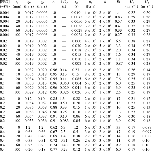
Rheological parameters of the salted (NaCl) 0.1 wt% HPAM solutions used in curtain experiments, where
 $t_{d}$
is the time of degradation (top) which is unknown for the last liquid (bottom) where salt is added after each PIV measurement. The first columns are similar to table 1 and the solvent viscosity is
 $\unicode[STIX]{x1D702}_{s}=0.001~\text{Pa}~\text{s}$
.
 $\mathit{El}$
is the Elasticity number (5.29),
 $U_{s}=q/2a$
is the extrusion velocity where
 $q$
is the linear flow rate and
 $U_{1}=U(z_{1})$
is the liquid velocity measured at
 $z_{1}\approx 2.5~\text{mm}$
from the slot, i.e. after swelling.

Rheological parameters of the PEO solutions with 40 wt% PEG solvent used in curtain experiments. The first columns are similar to table 1 and the solvent viscosity is
 $\unicode[STIX]{x1D702}_{s}=0.14~\text{Pa}~\text{s}$
.
 $\mathit{El}$
is the Elasticity number (5.29),
 $U_{s}=q/2a$
is the extrusion velocity where
 $q$
is the linear flow rate and
 $U_{1}=U(z_{1})$
is the liquid velocity measured at
 $z_{1}\approx 2.5~\text{mm}$
from the slot, i.e. after swelling.

Rheological properties of the liquid used as a reference for the investigations on die swell (§§ 4.6 and 6.1), and on the role of flow rate (§ 4.4) and die geometry (see § 6.3). All these experiments were performed the same day. This liquid is close to (but not exactly the same as) the degraded (
 $t_{d}=100~\text{min}$
) 0.4 wt% PEO solution with 20 wt% PEG solvent presented in table 2. Density is
 $\unicode[STIX]{x1D70C}=1026~\text{kg}~\text{m}^{-3}$
, surface tension is
 $\unicode[STIX]{x1D6FE}=62~\text{mN}~\text{m}^{-1}$
, solvent viscosity is
 $\unicode[STIX]{x1D702}_{s}=0.017~\text{Pa}~\text{s}$
and
 $\mathit{El}$
is the Elasticity number (5.29).

The MHS equation for aqueous unsalted solutions of HPAM molecules with hydrolysis degree 30 % is
 $[\unicode[STIX]{x1D702}]=0.022M^{0.74}$
(Wu et al.
Reference Wu, Hunkeler, Hamielec, Pelton and Woods1991; Kawale et al.
Reference Kawale, Marques, Zitha, Kreutzer, Rossen and Boukany2017). We obtain
 $[\unicode[STIX]{x1D702}]\approx 5.0~\text{m}^{3}~\text{kg}^{-1}$
and therefore
 $c^{\ast }=0.77/[\unicode[STIX]{x1D702}]\approx 0.15~\text{kg}~\text{m}^{-3}$
(equivalently 0.015 wt%), as well as
 $\unicode[STIX]{x1D708}=0.58$
. Hence,
 $c/c^{\ast }\approx 6.7$
for HPAM solutions without salt and polymer molecules are probably in the semi-dilute entangled regime. Since
 $c^{\ast }$
increases when adding salt (Chen et al.
Reference Chen, Yao, Liu, Luo, Zhou and Jiang2012), salted solutions are expected to be less entangled.
A.2 Discussion on the rheological parameters
The CaBER extensional relaxation time
 $\unicode[STIX]{x1D70F}_{fil}$
is compared in figure 27(b) with the relaxation times
 $\unicode[STIX]{x1D6F9}/2\unicode[STIX]{x1D702}_{p}$
calculated for PEO solutions exhibiting quadratic first normal stress differences
 $N_{1}=\unicode[STIX]{x1D6F9}\dot{\unicode[STIX]{x1D6FE}}^{2}$
(i.e. in the dilute and semi-dilute unentangled regimes). Both quantities are plotted against
 $c/c^{\ast }$
. While
 $\unicode[STIX]{x1D70F}_{fil}$
increases with polymer concentration,
 $\unicode[STIX]{x1D6F9}/2\unicode[STIX]{x1D702}_{p}$
decreases since
 $\unicode[STIX]{x1D702}_{p}$
increases faster than
 $\unicode[STIX]{x1D6F9}$
which scales as
 $\unicode[STIX]{x1D6F9}\propto c^{0.72}$
in the dilute regime and
 $\unicode[STIX]{x1D6F9}\propto c^{1.5}$
in the semi-dilute unentangled regime. The link between the first normal stress coefficient
 $\unicode[STIX]{x1D6F9}$
and the CaBER extensional relaxation time
 $\unicode[STIX]{x1D70F}_{fil}$
is far from obvious. An intensive study by Zell et al. (Reference Zell, Gier, Rafai and Wagner2010) involving semi-dilute PEO solutions in water–glycerol mixtures has been dedicated to this topic. The authors also report that
 $\unicode[STIX]{x1D6F9}\propto c^{1.5}$
for
 $c^{\ast }<c<c_{e}$
, as well as values of
 $\unicode[STIX]{x1D70F}_{fil}$
much larger than
 $\unicode[STIX]{x1D6F9}/2\unicode[STIX]{x1D702}_{p}$
. Our experiments suggest that
 $\unicode[STIX]{x1D70F}_{fil}\propto c^{0.84}$
, which is in agreement with the exponents found by Zell et al. (Reference Zell, Gier, Rafai and Wagner2010). The authors also report an empirical relation
 $\unicode[STIX]{x1D6F9}\propto \unicode[STIX]{x1D70F}_{fil}^{2}$
where, surprisingly, the prefactor does not depend on polymer concentration. Our experimental results follow the same quadratic dependence in the semi-dilute regime with a prefactor 0.06 Pa which is comparable to the prefactor reported by the authors.
Both relaxation times are compared in figure 27(b) with the Zimm (longest) relaxation time which is given by (Tirtaatmadja et al. Reference Tirtaatmadja, McKinley and Cooper-White2006)
 $$\begin{eqnarray}\unicode[STIX]{x1D70F}_{Z}=\frac{1}{\unicode[STIX]{x1D701}(3\unicode[STIX]{x1D708})}\frac{[\unicode[STIX]{x1D702}]M_{w}\unicode[STIX]{x1D702}_{s}}{{\mathcal{N}}_{A}k_{B}T},\end{eqnarray}$$
where
 $\unicode[STIX]{x1D701}$
is the Riemann zeta function,
 ${\mathcal{N}}_{A}$
is Avogadro’s number and
 $k_{B}$
is the Boltzmann constant. The prefactor is 0.38 for
 $\unicode[STIX]{x1D708}=0.5$
and 0.46 for
 $\unicode[STIX]{x1D708}=0.55$
and the corresponding values of
 $\unicode[STIX]{x1D70F}_{Z}$
are respectively 0.020 s and 0.024 s. The fact that
 $\unicode[STIX]{x1D70F}_{fil}$
is larger than
 $\unicode[STIX]{x1D70F}_{Z}$
in the dilute regime (
 $c<c^{\ast }$
) has been reported by Tirtaatmadja et al. (Reference Tirtaatmadja, McKinley and Cooper-White2006) and discussed by Clasen et al. (Reference Clasen, Plog, Kulicke, Owens, Macosko, Scriven, Verani and McKinley2006). The interpretation is that polymer chain–chain interactions (neglected in the Zimm model) are not negligible during the filament thinning process since
 $\unicode[STIX]{x1D70F}_{fil}\dot{\unicode[STIX]{x1D716}}=2/3$
which is larger than the coil–stretch transition value
 $1/2$
(De Gennes Reference De Gennes1974). The polymer chains are therefore highly extended and may overlap. Clasen et al. (Reference Clasen, Plog, Kulicke, Owens, Macosko, Scriven, Verani and McKinley2006) suggested that there must be an effective critical overlap concentration in extensional measurements which is orders of magnitude smaller than the conventional coil overlap concentration
 $c^{\ast }$
. Furthermore, the authors show that
 $\unicode[STIX]{x1D70F}_{fil}$
is larger than the longest relaxation time measured from small amplitude oscillatory shear (SAOS) experiments since intermolecular interactions are less important. The authors conclude that
 $\unicode[STIX]{x1D70F}_{fil}$
is an effective relaxation time which is relevant in strong extensional flows. CaBER experiments have indeed been used to determine the relevant polymer time scale in many elongational flows including spraying (Keshavarz et al.
Reference Keshavarz, Sharma, Houze, Koerner, Moore, Cotts, Threlfall-Holmes and McKinley2015), jetting (Clasen et al.
Reference Clasen, Bico, Entov and McKinley2009) contraction (Rodd et al.
Reference Rodd, Scott, Boger, Cooper-White and McKinley2005, Reference Rodd, Scott, Cooper-White, Boger and McKinley2007) and coating (curtain) flows (Becerra & Carvalho Reference Becerra and Carvalho2011; Karim et al.
Reference Karim, Suszynski, Griffith, Pujari, Francis and Carvalho2018b
). Note that we measure values of
 $\unicode[STIX]{x1D70F}_{fil}$
lower than
 $\unicode[STIX]{x1D70F}_{Z}$
for the two most dilute PEO solutions, as also reported by Clasen et al. (Reference Clasen, Plog, Kulicke, Owens, Macosko, Scriven, Verani and McKinley2006). The interpretation is that, for very dilute solutions, polymeric stress may be insufficient to maintain the elastocapillary balance leading to (3.3) and to allow an unambiguous determination of the longest relaxation time. Another possible interpretation is that our estimation of
 $\unicode[STIX]{x1D70F}_{Z}$
is incorrect due to mechanical degradation during sample preparation which leads to a lower average molecular weight
 $M_{w}$
.
We can compare the experimental values of the finite extensibility parameter
 $b$
to the microscopic expression (Clasen et al.
Reference Clasen, Plog, Kulicke, Owens, Macosko, Scriven, Verani and McKinley2006)
 $$\begin{eqnarray}b=3\left[\frac{j(\sin (\unicode[STIX]{x1D703}/2))^{2}M_{w}}{C_{\infty }M_{u}}\right]^{2(1-\unicode[STIX]{x1D708})},\end{eqnarray}$$
which involves the C–C bond angle
 $\unicode[STIX]{x1D703}=109^{\circ }$
, the number of bonds
 $j$
of a monomer unit with molar mass
 $M_{u}$
and the characteristic ratio
 $C_{\infty }$
. For PEO,
 $j=3$
and
 $C_{\infty }=4.1$
(Brandrup et al.
Reference Brandrup, Immergut, Abe and Bloch1989). Therefore, using
 $\unicode[STIX]{x1D708}=0.55$
gives a value
 $b=8.8\times 10^{4}$
which is very close to the values measured for dilute PEO solutions. Using
 $\unicode[STIX]{x1D708}=0.5$
gives a larger value
 $b=2.7\times 10^{5}$
.
Some scalings can be extracted from the data of table 1. According to Stelter et al. (Reference Stelter, Brenn, Yarin, Singh and Durst2002), the terminal extensional viscosity
 $\unicode[STIX]{x1D702}_{E}$
is proportional to
 $\unicode[STIX]{x1D70F}_{fil}$
with a prefactor which is larger for flexible polymers than for rigid polymers. Our data indeed suggest
 $\unicode[STIX]{x1D702}_{E}\propto \unicode[STIX]{x1D70F}_{fil}$
with a prefactor
 $8\times 10^{3}~\text{Pa}$
for solutions of flexible chains such as PEO and salted HPAM and with a lower prefactor for unsalted HPAM solutions. The data of table 1 also suggest a link between the degree of shear thinning
 $n$
and the effective value of the finite extensibility parameter
 $b$
. Indeed, solutions of flexible polymers correspond to large values of
 $b$
with
 $n$
close to 1 while shear-thinning solutions correspond to low values of
 $b$
. For both PEO and HPAM solutions we find the following empirical formula:
 $n\approx 0.16b^{0.17}$
for
 $b<5\times 10^{4}$
and
 $n=1$
for
 $b\geqslant 5\times 10^{4}$
. This link is not predicted by dilute polymer solutions models such as the FENE-P model which gives
 $\unicode[STIX]{x1D702}-\unicode[STIX]{x1D702}_{s}\propto \dot{\unicode[STIX]{x1D6FE}}^{-2/3}$
at large shear rates, i.e.
 $n=1/3$
for all values of
 $b$
.