Multiferroic materials form an exciting type of materials which can have multiple ferroic properties in the same phase^[Reference Spaldin and Fiebig^1, Reference Ramesh and Spaldin^2] such as (anti)ferromagnetism, ferroelectricity, ferroelasticity, etc. Out of the different kinds of multiferroics, the ones possessing both ferroelectric and magnetic orders have drawn particular attention.^[Reference Wojdel and Iñiguez^3–Reference Benedek and Fennie^6] This is because the magneto-electric coupling between these two orders can lead to the control of magnetism by electric field, or, vice versa, to the manipulation of electric properties by the application of magnetic field (such control is attractive for the design of original devices and is also of academic interest). One particularly known and important example of such coupling is provided by the so-called spin–current model^[Reference Katsura, Nagaosa and Balatsky^7, Reference Raeliarijaona, Singh, Fu and Bellaiche^8] for which the interaction energy is given by

(1)$$\Delta E = - C\lpar {\bf P} \times {\bf e}_{{\bf ij}} \rpar \cdot \lpar {\bf m}_{\bf i} \times {\bf m}_{\bf j} \rpar \comma$$

where P is the electric polarization, e_ij is the unit vector along a specific direction joining site i to site j and where m_i and m_j are the magnetic moments located at these sites i and j, respectively. C is a coefficient characterizing the strength of this spin–current interaction.^[Reference Katsura, Nagaosa and Balatsky^7, Reference Raeliarijaona, Singh, Fu and Bellaiche^8] Note that the spin–current model can also be seen as a Dzyaloshinsky–Moriya (DM) interaction,^[Reference Dzyaloshinsky^9, Reference Kimura, Goto, Shintani, Ishizaka, Arima and Tokura^10] which is given by D′ · (m_i × m_j), with the DM vector, D′, being equal to −C(P × e_ij). For instance, the spin–current model was advocated^[Reference Katsura, Nagaosa and Balatsky^7] to explain the occurrence of a spontaneous electric polarization at the temperature at which Mn spins form some spiral order in orthorhombically distorted multiferroics such as TbMnO₃, DyMnO₃, and GdMnO₃.^[Reference Kimura, Goto, Shintani, Ishizaka, Arima and Tokura^11] Similarly, the spin–current model has been proposed as one possible mechanism behind the clear correlation between the spin-helicity and the electronic polarization found in neutron diffraction measurements in Gd_0.7Tb_0.3MnO₃.^[Reference Yamasaki, Sagayama, Abe, Arima, Sasai, Matsuura, Hirota, Okuyama, Noda and Tokura^12] This spin–current model has also been recently shown^[Reference Lebeugle, Colson, Forget, Viret, Bataille and Gukasov^13, Reference Rahmedov, Wang, Iniguez and Bellaiche^14] to be responsible for the polarization-induced formation of the magnetic cycloid.^[Reference Lebeugle, Colson, Forget, Viret, Bataille and Gukasov^13,Reference Sosnowska, Loewenhaupt, David and Ibberson^15–Reference Catalan and Scott^27] It is of common wisdom to consider that (long-time-sought and desired) high magneto-electric coupling will be achieved when finding systems possessing a large value for the C coefficient appearing in Eq. (1). However, in that situation, it is also legitimate to ask two other important and currently unresolved question that are: (1) can large C values give rise to novel types of magnetic organization with respect to those of small or intermediate C? and (2) is the structural ground state affected by a large C coefficient? If yes, determining the microscopic origins of such effects is also of obvious importance.

The aim of this letter is to address these issues, by varying the strength of the spin–current interaction in the effective Hamiltonian approach of BFO (which is our present toy model). As we will see, surprises are in store. For instance, large C values lead to the formation of a previously unknown magnetic cycloid that propagates along an unusual low-symmetry direction. They also generate a structural phase transition from a polar high-symmetry phase to a polar low-symmetry state that is associated with a magnetically induced rotation of the electrical polarization. These striking features arise from a remarkable self-organization between different individual solutions of the spin–current model.

Let us first recall that the total energy corresponding to the effective Hamiltonian of BFO is expressed as:^[Reference Rahmedov, Wang, Iniguez and Bellaiche^14]

(2)$$\eqalign{E_{\rm tot} &= E_{{\rm FE} - {\rm AFD}} \lpar \lcub {\bf u}_i \rcub \comma \; \lcub \eta _i \rcub \comma \; \lcub \omega _i \rcub \rpar \cr & \quad + E_{\rm Mag} \lpar \lcub {\bf m}_i \rcub \comma \; \lcub {\bf u}_i \rcub \comma \; \lcub \eta _i \rcub \comma \; \lcub \omega _i \rcub \rpar,}$$

where the first part contains all non-magnetic variables: the local mode (u_i) that is directly proportional to the electric dipole centered in the unit cell i;^[Reference Zhong, Vanderbilt and Rabe^28] the strain in this unit cell (η_i) that gathers both homogeneous and inhomogeneous contributions;^[Reference Zhong, Vanderbilt and Rabe^28] and the antiferrodistortive rotational mode (ω_i) that is associated with oxygen octahedral tilting in unit cell i. All these variables are centered on Fe sites. The second term in the total energy is the magnetic-dependent term. It includes the mutual interaction between magnetic moments of Fe ions at different cells i (m_i) that all have a fixed magnitude of 4μ_B. It also contains interactions between magnetic moments and the other degrees of freedom (namely, local modes, antiferrodistortive motions, and strains). The analytical form of E _Mag is same as in Ref.,^[Reference Rahmedov, Wang, Iniguez and Bellaiche^14] and is thus given by:

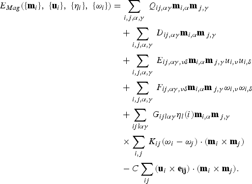(3)$$\eqalign{E_{Mag} \lpar \lcub {\bf m}_i \rcub \comma \; \lcub {\bf u}_i \rcub \comma \; \lcub \eta _i \rcub \comma \; \lcub \omega _i \rcub \rpar &= \sum\limits_{i\comma j\comma \alpha \comma \gamma } \, Q_{ij\comma \alpha \gamma } {\bf m}_{i\comma \alpha } {\bf m}_{\,j\comma \gamma } \cr & \quad + \sum\limits_{i\comma j\comma \alpha \comma \gamma } \, D_{ij\comma \alpha \gamma } {\bf m}_{i\comma \alpha } {\bf m}_{\,j\comma \gamma } \cr & \quad + \sum\limits_{i\comma j\comma \alpha \comma \gamma } \, E_{ij\comma \alpha \gamma \comma \nu \delta } {\bf m}_{i\comma \alpha } {\bf m}_{\,j\comma \gamma } u_{i\comma \nu } u_{i\comma \delta } \cr & \quad + \sum\limits_{i\comma j\comma \alpha \comma \gamma } \, F_{ij\comma \alpha \gamma \comma \nu \delta } {\bf m}_{i\comma \alpha } {\bf m}_{\,j\comma \gamma } \omega _{i\comma \nu } \omega _{i\comma \delta } \cr & \quad + \sum\limits_{ijl\alpha \gamma } \, G_{ijl\alpha \gamma } \eta _l \lpar i\rpar {\bf m}_{i\comma \alpha } {\bf m}_{\,j\comma \gamma } \cr & \quad \times \sum\limits_{i\comma j} \, K_{ij} \lpar \omega _i - \omega _j \rpar \cdot \lpar {\bf m}_i \times {\bf m}_j \rpar \cr & \quad - C\sum\limits_{ij} \, \lpar {\bf u}_i \times {\bf e}_{{\bf ij}} \rpar \cdot \lpar {\bf m}_i \times {\bf m}_j \rpar.}$$

The first term in the above expression represents magnetic dipolar interaction where both indices i and j run over all the sites. The second term is the direct magnetic exchange between magnetic moments at sites i and j. The third, fourth, and fifth terms characterize the change in magnetic exchange interaction induced by the local modes, antiferrodistortive motions, and strains. The index j for the second, third, fourth, and fifth term runs over first, second, and third nearest neighbors of site i. The first five energies desire to induce a collinear magnetism. On the other hand, the sixth term, in which the j index runs over the six first nearest neighbors of site i, is at the origin of the spin-canted weak ferromagnetic structure of BFO, and involve the rotations of the oxygen octahedra.^[Reference Albrecht, Lisenkov, Ren, Rahmedov, Kornev and Bellaiche^29–Reference Wang, Weerasinghe and Bellaiche^32] The last term represents the spin–current model,^[Reference Katsura, Nagaosa and Balatsky^7, Reference Raeliarijaona, Singh, Fu and Bellaiche^8] and has been found to be essential to reproduce the complex cycloidal structure of BFO bulks.^[Reference Rahmedov, Wang, Iniguez and Bellaiche^14] To appreciate the results of the present study (to be discussed below), it is important to know that, for this last term, j runs over the 12 second nearest neighbors of site i, and e_ij is the unit vector along the direction joining site i to site j (for symmetry reasons, this sum has to run over all second-nearest-neighbor directions, since the reference state of our Taylor expansion of E _tot is the cubic paraelectric and paramagnetic state). Here, the coefficient C appearing in the last term is allowed to vary, to find the effect of such spin–lattice coupling on physical properties. As we will see, this variation can lead to new magnetic configurations, as well as anomalous behavior of the electrical polarization.

We have performed Monte Carlo (MC) simulations using the E _tot internal energy with a 12 × 12 × 12 supercell. The finite-temperature properties of the modeled bulk perovskite system are obtained using 10⁶ MC sweeps for equilibration and 10⁵ additional sweeps to calculate statistical averages.

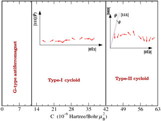
Figure 1 schematizes the different magnetic structures we numerically found at low temperature, when varying the C parameter. Below the critical value of 1.2 × 10⁻⁵ Hartree/Bohr μ_B², the magnetic ground state is the spin-canted structure reported in Refs. Reference Albrecht, Lisenkov, Ren, Rahmedov, Kornev and Bellaiche29–Reference Bellaiche, Gui and Kornev31, for which a large G-type antiferromagnetic vector coexists with a weak and perpendicular ferromagnetic vector.

Figure 1.

Range of the different magnetic structures numerically found when varying the spin–lattice coupling constant C. A snapshot of the different cycloids in their cycloidal plane is also provided by means of red arrows (the snapshot corresponds to C = 1.4 × 10⁻⁵ Hartree/Bohr μ_B² for the type-I cycloid and to C = 5.6 × 10⁻⁵ Hartree/Bohr μ_B² for the type-II cycloid). The directions of the cycloidal propagation, of the polarization and of the pseudo-cubic [111] axis are also schematized there, to emphasize the difference between the two cycloids.

Above this value and up to a coefficient C~4.2 × 10⁻⁵ Hartree/Bohr μ_B², the resulting magnetic dipoles organize themselves into the cycloidal configuration that is known to occur in BFO bulk,^[Reference Rahmedov, Wang, Iniguez and Bellaiche^14,Reference Sosnowska, Loewenhaupt, David and Ibberson^15–Reference Catalan and Scott^27] that is the magnetic dipoles (mostly) rotate in an $\lcub \bar 2 11\rcub $ plane possessing both the electrical polarization (that is oriented along the pseudo-cubic [111] direction) and one direction (i) joining second-nearest neighbors and (ii) being perpendicular to the electrical polarization (such as the pseudo-cubic $\lsqb 0\bar 11\rsqb $ direction). This direction joining second-nearest neighbors is spanned by one of the 12 e_ij vectors appearing in the last term of Eq. (3), and coincides with the propagation direction of the cycloid. Note that there is also a spin density wave, involving small out-of-plane components of the magnetic moments, that occurs in BFO bulks, in addition to the in-plane cycloid.^[Reference Rahmedov, Wang, Iniguez and Bellaiche^14, Reference Ramazanoglu, Laver, Ratcliff, Watson, Chen, Jackson, Kothapalli, Lee, Cheong and Kiryukhin^33] This cycloid will be denoted as “type-I cycloid” in the following.

Surprisingly, for larger values of the C coefficient, a novel magnetic structure emerges. It consists of another cycloidal configuration, to be referred to as “type-II cycloid”. Its propagation direction is now oriented along an unusual (low-symmetry) pseudo-cubic $ \lt 0\bar 12 \gt$ direction. The directions of propagation of the type-I and type-II cycloids were practically found by computing the Fourier transform of the magnetic dipoles for the different k-points that are allowed for the 12 × 12 × 12 supercell.^[Reference George, Iñiguez and Bellaiche^34] In the case of the type-I cycloid, the first Brillouin zone vector that possesses the largest component of the Fourier transform is given by ${{\bf k}_{\rm cyclo-I} = \displaystyle{{\lpar2\pi } / {12a_{\rm lat}\rpar }}}\lpar 6{\hat {\bf x}} + 5{\hat {\bf y}} - 5{\hat{\bf z}}\rpar $, where a_lat is the lattice constant of the primitive cell, and ${\hat{\bf x}}\comma \; {\hat{\bf y}}$, and ${\hat{\bf z}}$ are the unit vectors along three pseudo-cubic directions. This characterizes a propagation direction along the $\lsqb 0 \bar 11\rsqb $ direction. For the type-II cycloid, the corresponding vector is ${\bf k}_{\rm cyclo-II} = {\displaystyle{{\lpar2\pi } / {12a_{lat} \rpar}}}\lpar 6{\hat{\bf x}} + 5{\hat{\bf y}} - 4{\hat{\bf z}}\rpar $, which is inherent to a propagation direction being oriented along $\lsqb 0\bar 12\rsqb $. Note that Fe first-nearest-neighbors are antiferromagnetically coupled to each other in the type-II cycloid, as in the type-I cycloid. As seemingly at odds with any of the 12 different sums over j running in the last term of Eq. (3), this direction is therefore not lying anymore along any second-nearest neighbor direction. It is also not perpendicular to the polarization (which is lying close to [111])! Furthermore, the magnetic dipoles in the type-II cycloid are found to rotate within a $\lcub \bar 321\rcub $ plane that contains both the polarization and this novel cycloidal propagation direction.

Before trying to understand the origin(s) of this original magnetic cycloid, let us also investigate if the electrical polarization can be affected by the C coefficient. Consequently, Figs. 2(a)–2(c) show the evolution of the 〈u〉 supercell average of the local modes as a function of temperature for three different representatives values of C. They are, respectively, 7 × 10⁻⁶ Hartree/Bohr μ_B² (which leads to the spin-canted structure at low temperature), 2.8 × 10⁻⁵ Hartree/Bohr μ_B² (which results in the type-I cycloid at low temperature), and 6.3 × 10 ^− 5 Hartree/Bohr μ_B² (which generates a type-II cycloid at low temperature). One can see that for the two smallest C coefficients, a paraelectric–to-ferroelectric transition occurs at T _C about 1100 K, below which the polarization points along the pseudo-cubic [111] direction (since the x-, y-, and z-components of 〈u〉 are all equal to each other and non-null). The polarization remains oriented along [111] below the magnetic transition temperature, T _N ≃ 660 K. On the other hand, the third situation (corresponding to C = 6.3 × 10⁻⁵) is notably different from the first two cases for several reasons. First of all, T _C and T _N significantly increase by 96 K and 340 K, respectively. Such enhancement can be understood by realizing that the last term of Eq. (3) indicates that increasing the C coefficient favors both the formation of local modes (and hence of a polarization) and of the cross-product between magnetic moments at sites i and j (and hence of a cycloidal-type structure). Secondly, while the polarization remains oriented along the [111] pseudo-cubic direction between T _N and T _C, it rotates toward a low-symmetry [pqr] direction—with r < p < q—below T _N [note that, as shown in Fig. 2(c), the x and y components of the local modes are close to each other but are physically distinct, since their difference is found to be larger than their statistical error bars]. In other words, the occurrence of the type-II cycloid results in a structural transformation from a polar rhombohedral phase to a polar triclinic state! We are not aware that such type of strong magneto-electric effect, correlating the formation of magnetic ordering with a lowering of symmetry between polar phases and with rotation of the polarization, has ever been previously found (Note that Refs. [Reference Lebeugle, Colson, Forget, Viret, Bataille and Gukasov13, Reference Schmid35] suggested that the formation of the type-I cycloid in BFO would result in the transformation of a polar rhombohedral to a polar monoclinic state, but this interpretation is likely incorrect, since it is now known that BFO bulk remains in a rhombohedral R3c state below T _N). It is also worthwhile to know that the polarization in any of the three cases depicted in Fig. 2 is found to be perfectly homogeneous at low temperature. This implies that the breaking of symmetry between the x, y, and z components of the polarization seen in Fig. 2(c) do not originate from the formation of domains (having, e.g., small versus large z-component of the electric dipoles).

Figure 2.

Temperature dependence of the three Cartesian components of the supercell average of the local mode for three different values of the C coefficient. The magnetic and paraelectric–to–ferroelectric transition temperatures, T _N and T _C, are shown by dashed and solid vertical lines, respectively. Panel (a) corresponds to C = 7 × 10⁻⁶ Hartree/Bohr μ_B², which leads to the spin-canted magnetic structure below T _N. Panel (b) is associated with C = 2.8 × 10⁻⁵ Hartree/Bohr μ_B², which yields the type-I cycloid below T _N. Panel (c) represents the results for C = 6.3 × 10⁻⁵ Hartree/Bohr μ_B², whose value generates a type-II cycloid below T _N. It can be seen that the rhombohedral polar phase survives only for a small window of temperature (shown as Rhombo), before transforming to a triclinic polar state, for the largest shown C value.

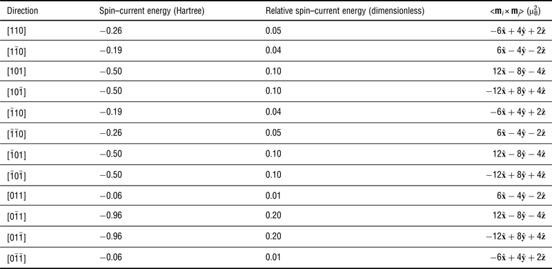
Let us now reveal why a type-II cycloid and a resulting low-symmetry structural ground state can occur for large C coefficient. For that Table I reports at low temperature and for C = 6.3 × 10⁻⁵ (i.e., when a type-II cycloid is in place): (i) the “spin–current” energy associated with each of the 12 second-nearest-neighbor directions that is the energy of each of these 12 directions appearing in the last term of Eq. (3); (ii) the resulting relative “spin–current” energy, which is defined as the “spin–current” energy divided by the total energy of the last term of Eq. (3), for each of these 12 second-nearest-neighbor directions; and (iii) the associated (averaged) m_i × m_j cross-product for each of these 12 directions. It is important to notice that (1) there are two (opposite) directions, i.e. $\lsqb 0 \bar 11\rsqb $ and $\lsqb 01\bar 1\rsqb $ that have the largest relative spin–current energy of the order w ≃ 0.20; (2) four other directions—that are [101], $\lsqb \bar 101\rsqb \comma \; \lsqb \bar 10 \bar 1\rsqb $ and $\lsqb 10\bar 1\rsqb $—have significant relative spin–current energies of approximately half the predominant one, w/2 ≃ 0.10; (3) out of these six directions, three of them (namely, $\lsqb 0\bar 11\rsqb $, [101], $\lsqb \bar 101\rsqb $) have an averaged m_i × m_j close to be $\zeta \simeq 4\lpar 3{\hat{\bf x}} - 2{\hat{\bf y}} - {\hat{\bf z}}\rpar $, whereas the other three have a nearly opposite averaged m_i × m_j. Taking into account items (1)–(3), only considering the six aforementioned directions (as shown in Table I, the other six second-nearest-neighbor directions have smaller relative spin–current energies, and thus can be neglected in first approximation) and using commutative properties of the mixed product allows the rewriting of the last term of Eq. (3) as

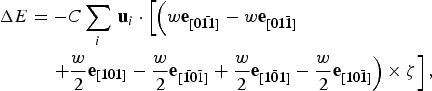(4)$$\eqalign{\Delta E &= - C\sum\limits_i \, {\bf u}_i \cdot \left[ \left({ w{\bf e}_{\lsqb {\bf 0} \bar {\bf 11}\rsqb} - w{\bf e}_{\lsqb {\bf 01} \bar {\bf 1}\rsqb} }\right. \right. \cr & \quad \left. \left. + \displaystyle{w \over 2}{\bf e}_{\lsqb {\bf 101}\rsqb } - \displaystyle{w \over 2}{\bf e}_{\lsqb \bar {\bf 10}\bar 1\rsqb } + \displaystyle{w \over 2}{\bf e}_{\lsqb \bar {\bf 101}\rsqb } - \displaystyle{w \over 2}{\bf e}_{\lsqb {\bf 10} \bar {\bf 1}\rsqb } \right)\times \zeta \right]\comma}$$

where ${\bf e}_{\lsqb {\bf 0} {\bar {\bf 11}}\rsqb }\comma \; {\bf e}_{\lsqb {\bf 01} \bar {\bf 1}\rsqb }\comma \; {\bf e}_{\lsqb {\bf 101}\rsqb }\comma \; {\bf e}_{\lsqb { \bar {\bf 10}}{\bar 1}\rsqb }\comma \; {\bf e}_{\lsqb {\bar {\bf 101}}\rsqb }\comma \; {\rm and} \;{\bf e}_{\lsqb {\bf 10} {\bar {\bf 1}}\rsqb }$ are unit vectors along the $\lsqb 0 \bar 11\rsqb \comma \; \lsqb 01\bar 1\rsqb \comma \; \lsqb 101\rsqb \comma \; \lsqb \bar 10\bar 1\rsqb $, and $\lsqb \bar 101\rsqb \comma \; \lsqb 10\bar 1\rsqb $ directions, respectively. As a result, Eq. (4) becomes:

(5)$$\Delta E = - \sqrt 2 Cw\sum\limits_i \, {\bf u}_i \cdot \left[{\left({ - {\hat{\bf y}} + 2{\hat{\bf z}}} \right)\times \zeta } \right].$$

Once knowing that we also numerically found that, in the type-II cycloid, the cross product m_i × m_j between two adjacent i and j sites along the $\lsqb 0\bar 12\rsqb $ direction is also equal to ζ, Eq. (5) then naturally explains why, in the type-II cycloid, (i) the propagation direction of the magnetic cycloid is now along $\lsqb 0\bar 12\rsqb $; and (ii) the magnetic moments rotate in the plane defined by (the homogeneous) u_i and $- {\hat{\bf y}} + 2{\hat{\bf z}}$. In other words, this type-II cycloid can be thought as being the result of a specific combination (i.e., with very specific weights) of different individual solutions of the spin–current model–each individual solution corresponding to a given second-nearest neighbor direction. In contrast, the type-I cycloid is associated with a single individual solution. We are not aware that such remarkable magnetic organization has ever been proposed or found in the literature. This combination occurs for large value of C because the last term of Eq. (3) indicates that the more second-nearest-neighbor directions participate in this term the most likely the corresponding energy can be lowered [note that not all the second-nearest-neighbor directions can equally participate in this last term, since this would lead to an exact cancellation of all the sums involved in the last term of Eq. (3) for an homogeneous polarization]. Interestingly, Eq. (5) also tells us why the polarization is not anymore along the [111] direction when the type-II cycloid forms. As a matter of fact, plugging the previously determined $\zeta \simeq 4\lpar 3{\hat {\bf x}} - 2{\hat{\bf y}} - {\hat{\bf z}}\rpar $ into this latter equation gives

(6)$$\Delta E = - \sqrt 2 Cw\sum\limits_i \, {\bf u}_i \cdot \left[{5{\hat{\bf x}} + 6{\hat{\bf y}} + 3{\hat{\bf z}}} \right].$$

Such formula can be thought as representing a coupling between the local electric dipoles Z*u_i (where Z* is the Born effective charge) and a “magnetically induced” electric field that is equal to ${\sc E} = {\textstyle{\lpar{\sqrt 2 Cw} / {Z^ \ast }\rpar}}\left[{5{\hat{\bf x}} + 6{\hat{\bf y}} + 3{\hat{\bf z}}} \right]$. As indicated by its Cartesian components, this electric field wants to favor a polarization having a larger y-component, a smaller z-component and an intermediate x-component. This is consistent with the simulations shown in Fig. 2(c), and therefore explains why the system becomes triclinic when the type-II cycloid forms. It is also very likely that such phase transition can lead to large physical responses since, e.g., giant piezoelectric and dielectric coefficients have been found in low-symmetry phases.^[Reference Noheda, Cox, Shirane, Gonzalo, Cross and Park^36–Reference Iñiguez and Bellaiche^41]

Table 1.

Low-temperature energies associated with the last term of the effective magnetic Hamiltonian (see text) and averaged m_i × m_j for the 12 different second nearest-neighbor directions, when the spin–lattice coupling constant C = 6.3 × 10⁻⁵. The Cartesian components of the averaged m_i × m_j have been rounded to integers. The quantities shown are those associated with a single snapshot of the type-II cycloid structure in a 12 × 12 × 12 simulation box.

In summary, our calculations reveal that, and explain why, original magnetic arrangements and an unusual, magnetically induced phase transition between a high-symmetry and a low-symmetry ferroelectric phase (that is accompanied by a rotation of the electrical polarization) can occur in systems possessing strong (spin–lattice) spin–current interactions. Note that we also incorporated Eq. (1) into the newly-developed effective Hamiltonian of Ref. Reference Prosandeev, Wang, Ren, Iñiguez and Bellaiche42 (that yields a Pnma phase at high temperature, unlike the effective Hamiltonian of Ref. Reference Rahmedov, Wang, Iniguez and Bellaiche14). This incorporation leads to the same original magnetic configuration and low-symmetry ferroelectric phase reported here for large C coefficient. This is consistent with the facts that this low-symmetry phase is derived from the R3c state, and that both effective Hamiltonians^[Reference Rahmedov, Wang, Iniguez and Bellaiche^14, Reference Prosandeev, Wang, Ren, Iñiguez and Bellaiche^42] correctly reproduce this R3c state (or, equivalently that the new terms introduced in Ref. Reference Prosandeev, Wang, Ren, Iñiguez and Bellaiche42 to generate the Pnma phase vanish in the R3c phase). Discovering such systems may occur by either (i) considering multiferroic nanostructures, since, e.g., BFO films under various epitaxial conditions have been recently found to exhibit three different magnetic configurations;^[Reference Sando, Agbelele, Rahmedov, Liu, Rovillain, Toulouse, Infante, Pyatakov, Fusil, Jacquet, Carretero, Deranlot, Lisenkov, Wang, Le Breton, Cazayous, Sacuto, Juraszek, Zvezdin, Bellaiche, Dkhil, Barthlmy and Bibes^43] or (ii) by studying multiferroics made of elements having strong spin–orbit coupling, because this latter coupling is at the heart of the spin–current model^[Reference Katsura, Nagaosa and Balatsky^7, Reference Raeliarijaona, Singh, Fu and Bellaiche^8, Reference Rahmedov, Wang, Iniguez and Bellaiche^14] [note that transitions from low-spin to high-spin state should also result in an increase of the strength of the spin–current interaction, or, conversely, reducing the magnitude of the magnetic moments can be thought as reducing the strength of the spin–current interaction, according to Eq. (1)]. We therefore hope that the present work will encourage the discovery of such multiferroics, and deepens the current knowledge of these fascinating materials.