1 Introduction
The capillary instability of a liquid jet in an ambient medium has been of scientific and industrial interest for more than a century. After the pioneering experiments of Savart (Reference Savart1833) and Plateau (Reference Plateau1873), Rayleigh (Reference Rayleigh1878) was the first to study theoretically the linear capillary instability of an inviscid liquid jet in a vacuum. In a further investigation, Rayleigh (Reference Rayleigh1892) considered the effect of liquid viscosity. The viscous dispersion relation was derived for any possible viscosity and the solution for the paramount viscosity was determined. Rayleigh’s analysis was then generalised by Weber (Reference Weber1931) and Chandrasekhar (Reference Chandrasekhar1961) to represent all intermediate viscous cases.
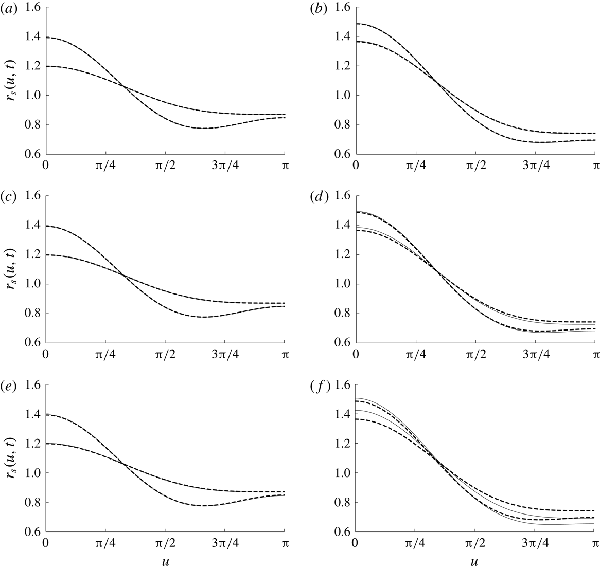
Liquid jet experiments showed that linear stability analyses are appropriate to predict the growth rate of the jet surface deformation (Goedde & Yuen Reference Goedde and Yuen1970; Rutland & Jameson Reference Rutland and Jameson1971; Blaisot & Adeline Reference Blaisot and Adeline2000; Gonzales & Garcia Reference Gonzales and Garcia2009; Charpentier et al. Reference Charpentier, Renoult, Crumeyrolle and Mutabzi2017) and the size of the main drops (Rutland & Jameson Reference Rutland and Jameson1970; Charpentier et al. Reference Charpentier, Renoult, Crumeyrolle and Mutabzi2017). However, these analyses fail to predict the formation of satellite drops, i.e. the small drops observed in the experiments as illustrated in figure 1. This phenomenon has been very early interpreted as a nonlinear effect (Rutland & Jameson Reference Rutland and Jameson1970).
Liquid jet breakup leading to the formation of satellite drops. From top to bottom:
 $k=0.075$
,
 $k=0.250$
,
 $k=0.683$
where
 $k$
is the wavenumber non-dimensionalised by the jet radius (Rutland & Jameson (Reference Rutland and Jameson1971), reproduced with permission).

Satellite drop formation in water jet breakup was studied experimentally, among others, by Vassallo & Ashgriz (Reference Vassallo and Ashgriz1991) for different values of imposed disturbance wavenumbers. It was observed that, for the
 $k$
domain
 $0.57<k<1$
, with
 $k$
the wavenumber non-dimensionalised by the jet radius, no satellite drops may be formed. This observation is in contrast to the experimental results of Rutland & Jameson (Reference Rutland and Jameson1970) (as illustrated in figure 1 for
 $k=0.683$
) and Lafrance (Reference Lafrance1975) who observed satellite drops up to
 $k\approx 0.73$
. Experimental results on satellite drop formation are known to be sparse.
A theoretical prediction of satellite drop formation in liquid jet breakup requires a nonlinear stability analysis. Since the development of spatial instability is of minor importance for jet-radius-based Weber numbers of approximately 80 and higher (Keller, Rubinow & Tu Reference Keller, Rubinow and Tu1973), which are easily reached in many applications, we restrict our discussion to temporal instability. A recent weakly nonlinear analysis and numerical simulation of spatial jet instability is due to Xie, Yang & Ye (Reference Xie, Yang and Ye2017). The nonlinear analysis reveals disturbance growth rates that depend on the initial dimensionless amplitude, the dimensionless wavenumber of the disturbance and the liquid jet Ohnesorge number. These are the three dimensionless parameters of the temporal stability analysis discussed in the present work.
The first weakly nonlinear temporal stability analysis of a liquid jet is due to Yuen (Reference Yuen1968). He treated the jet liquid as inviscid and the liquid velocity field as irrotational. The flow field quantities were expanded in series of powers of a small amplitude parameter, and the analysis was carried out to third order in the expansion parameter, where a correction to the cutoff wavenumber between the unstable and stable regimes comes in (Eggers Reference Eggers1997). Yuen applied the method of multiple time scales to avoid secular terms in the third-order solution. For
 $k=0.3$
, Yuen (Reference Yuen1968) found secondary waves leading to the formation of satellite drops in the jet breakup. For
 $k=0.7$
and
 $k=0.95$
, secondary waves are not observed, indicating that satellite drop formation predicted by the model depends on the deformation wavenumber. A careful experimental validation of Yuen’s theory is due to Taub (Reference Taub1976). Nayfeh (Reference Nayfeh1970) presented an alternative formulation of a third-order perturbation expansion for the instability of an incompressible, inviscid liquid jet. Using the method of multiple time scales, Nayfeh arrives at a solution similar to Yuen, but with the influence of the perturbation amplitude on the cutoff wavenumber correctly represented, since the secular terms were completely avoided (Eggers Reference Eggers1997).
Lafrance (Reference Lafrance1975) presented Yuen’s theory again and used it for predicting satellite drop sizes in capillary liquid jet breakup. The theory is found to well represent water jet breakup at disturbance wavenumbers between 0.1 and 0.9 in that measured sizes of main and satellite drops agree well with the theoretical predictions. The same holds true for the growth rate of the jet surface deformation. Eggers (Reference Eggers1997), however, reports algebraic errors in Lafrance’s theory, which is complemented by our finding that Lafrance (Reference Lafrance1975) used Yuen’s equations, which were partly mistyped in his publication, for his calculations, while Yuen himself used the correct equations. The good agreement of water jet experiments with Rayleigh’s dispersion relation when measuring relative displacements of jet swells and necks is claimed by Goedde & Yuen (Reference Goedde and Yuen1970) to be due to the cancellation of nonlinear terms.
Eggers (Reference Eggers1997) points at differences between the results for the cutoff wavenumber between the unstable and stable regimes by Yuen (Reference Yuen1968), Nayfeh (Reference Nayfeh1970) and Lafrance (Reference Lafrance1975). Nonlinearity produces an asymmetric evolution of an initially sinusoidal wave with generation of higher harmonics, as well as feedback into the fundamental wave (Yuen Reference Yuen1968). The difference between the two dependencies of the cutoff on the disturbance amplitude predicted by Yuen and Nayfeh are traced back to a secular term overlooked by Yuen. The analysis by Lafrance (Reference Lafrance1975) predicted no dependency of the cutoff on the disturbance amplitude at all. Chaudhary & Redekopp (Reference Chaudhary and Redekopp1980) showed that this was due to an error in the algebra of Lafrance’s analysis (Eggers Reference Eggers1997).
Eggers & Dupont (Reference Eggers and Dupont1994) analysed drop formation in a quasi-one-dimensional approximation of the Navier–Stokes equations. The Taylor-series expansions of the velocity components and pressure in the liquid allow for solutions close to the singularity at jet breakup, which weakly nonlinear analyses do not offer. The resulting equations for the expansion coefficients as functions of the axial coordinate are solved numerically. Deformed jet states with drop formation computed, close to pinch off, compare very well with experimental flow visualisation, both for water and glycerol, with viscosities different by a factor of approximately 1000.
Papageorgiou (Reference Papageorgiou1995) developed similarity solutions for the instability of inviscid and viscous liquid jets, accounting for drop pinch off and the jet dynamics beyond the instant of drop formation. Among the viscous jets, distinction is made between the Stokes and the Navier–Stokes cases, according to very small or large values of a non-dimensional number termed the Reynolds number, which is the inverse of the Ohnesorge number squared. The jets are treated as slender, i.e. their radial extension is much smaller than the axial one. The similarity solutions are not based on an arbitrary axial length scale, in contrast to the one-dimensional equations used by earlier investigators. This work by Papageorgiou (Reference Papageorgiou1995) generalizes the work by Keller & Miksis (Reference Keller and Miksis1983) and Ting & Keller (Reference Ting and Keller1990), who investigated inviscid jets and sheets only. Results of Papageorgiou’s work rather consist of the evolution of the jet surface shape with time rather than, e.g. drop sizes. The inclusion of the jet behaviour around the pinching singularity makes this work and the work by Eggers & Dupont (Reference Eggers and Dupont1994) very attractive for the description of the drop formation process.
Mansour & Lundgren (Reference Mansour and Lundgren1990) simulated numerically the capillary breakup of a liquid jet at varying wavelength of the initial jet deformation. The computations based on a boundary integral method treat cases with very small jet Ohnesorge numbers, i.e. nearly inviscid liquid jets. Dynamic interaction between the jet and the ambient medium is not accounted for. The formation of large drops separated by smaller drops is obtained. The initial disturbance growth rate is found to agree with Rayleigh’s linear theory. Satellite drops form at all unstable disturbance wavelengths, in contrast to the finding of the weakly nonlinear analysis by Yuen (Reference Yuen1968). Comparison with the experiment shows that the simulation slightly underestimates main drop sizes and overestimates satellite drop sizes.
A study of temporal capillary jet instability based on numerical solutions is due to Ashgriz & Mashayek (Reference Ashgriz and Mashayek1995). The Navier–Stokes equations for the jet with free surface and surface tension are solved, using a Galerkin finite-element method and applying an interface capturing scheme. The jet surface is initially deformed sinusoidally and then tracked with ongoing time. The breakup is found to occur in the middle between two swells on the jet only for very low Reynolds numbers, which are in fact inverse Ohnesorge numbers. For larger Reynolds numbers, breakup rather occurs close to the swells, leaving a section of the jet which forms satellite drops. Satellite drop formation is found to occur for all the dimensionless disturbance wavenumbers between 0.2 and 0.9, and the satellite size decreases with increasing wavenumber. Growth rate measurements are compared to results from linear viscous theory, showing that the theory predicts the numerical results better for higher Ohnesorge numbers. The linear theory rather overestimates the measured growth rate at lower wavenumbers, and underestimates it at higher wavenumbers. The largest deviation at a Ohnesorge number of
 $5\times 10^{-3}$
is approximately 10 %. The deviation from linear theory is reduced when the growth rate measurement is performed with a two-mode fitting, taking into account the two capillary modes, as shown in figure 12 of Gonzales & Garcia (Reference Gonzales and Garcia2009) for three wavenumbers
 $k=0.2$
,
 $k=0.7$
and
 $k=0.9$
. The study of the influence of wavenumber on growth rate measurements was completed in a recent multi-scale analysis of simulated low Ohnesorge liquid jets by Dumouchel et al. (Reference Dumouchel, Aniszewski, Vu and Ménard2017), for which the agreement between linear theory and growth rate measurements performed with a single-mode fitting was found to be excellent, independently of the wavenumber (see figure 10 of that paper).
In the present work we conduct a weakly nonlinear temporal stability analysis of a viscous jet, which is missing in the literature, to gain insight into the role of the liquid viscosity on the formation of satellite drops. This model is a counterpart of the ones developed by Yuen (Reference Yuen1968) for inviscid liquid jets and by Yang et al. (Reference Yang, Wang, Fu, Du and Tong2013) for viscous liquid sheets. Since satellite drop formation is initially due to the growth of the first nonlinear contribution to the jet deformation (see Renoult, Rosenblatt & Carles (Reference Renoult, Rosenblatt and Carles2015) for more details on the effects of nonlinearity on a fluid interface instability), the jet surface shape is expanded up to second order in the small initial amplitude deformation. The present work details and extends the short contribution by Renoult, Brenn & Mutabazi (Reference Renoult, Brenn, Mutabazi, Payri and Margot2017) to the ILASS Europe conference 2017.
In the following section we derive the equations of motion and their boundary and initial conditions to second order in the initial deformation amplitude. Thereafter we solve the equations derived in the sequence of the order. The solutions are then presented and discussed by comparison to the inviscid solution and to previous numerical and experimental studies. The paper ends with the conclusions.
2 The problem and the equations
The weakly nonlinear temporal analysis of the capillary instability of a liquid jet is studied. The jet is assumed to be symmetric around the axial direction of the cylindrical coordinate system. The liquid is treated as incompressible and Newtonian. The dynamic influence from the ambient fluid is neglected and body forces are not accounted for.
Initially, the jet is deformed from the circular cylindrical shape by a single-mode perturbation of wavenumber
 $k=2\unicode[STIX]{x03C0}/\unicode[STIX]{x1D706}$
(with
 $\unicode[STIX]{x1D706}$
the wavelength of the perturbation) and amplitude
 $\unicode[STIX]{x1D702}_{0}$
and is at rest, as sketched in figure 2. The amplitude parameter,
 $\unicode[STIX]{x1D702}_{0}$
, is assumed to be small compared to the radius of the unperturbed jet,
 $a$
. More arbitrary initial conditions are discussed in the generalised normal-mode linear analysis of Garcia & Gonzales (Reference Garcia and Gonzales2008).
The purpose of the temporal analysis is to determine the time evolution of the small-amplitude perturbation on the jet surface, velocity field and pressure field in the liquid flow. To that end, the jet surface is described by
 $r_{s}(z,t)=a+\unicode[STIX]{x1D702}(z,t)$
, where
 $\unicode[STIX]{x1D702}$
is the deformation against the undisturbed cylindrical jet of radius
 $a$
, the pressure field by
 $p(r,z,t)$
and the velocity field by the two components
 $u_{r}(r,z,t)$
and
 $u_{z}(r,z,t)$
, taking advantage of the axisymmetry for the problem studied here.
The fluid variables and equations are non-dimensionalised with the undeformed jet radius
 $a$
, the capillary time scale
 $(\unicode[STIX]{x1D70C}a^{3}/\unicode[STIX]{x1D70E})^{1/2}$
and the capillary pressure
 $\unicode[STIX]{x1D70E}/a$
for length, time and pressure, respectively. Here,
 $\unicode[STIX]{x1D70C}$
is the liquid density and
 $\unicode[STIX]{x1D70E}$
the surface tension.
The continuity equation and the two components of the momentum equation in the radial
 $(r)$
and axial
 $(z)$
directions read
 $$\begin{eqnarray}\displaystyle & \displaystyle \frac{1}{r}\frac{\unicode[STIX]{x2202}}{\unicode[STIX]{x2202}r}(ru_{r})+\frac{\unicode[STIX]{x2202}u_{z}}{\unicode[STIX]{x2202}z}=0, & \displaystyle\end{eqnarray}$$
 $$\begin{eqnarray}\displaystyle & \displaystyle \frac{\unicode[STIX]{x2202}u_{r}}{\unicode[STIX]{x2202}t}+u_{r}\frac{\unicode[STIX]{x2202}u_{r}}{\unicode[STIX]{x2202}r}+u_{z}\frac{\unicode[STIX]{x2202}u_{r}}{\unicode[STIX]{x2202}z}=-\frac{\unicode[STIX]{x2202}p}{\unicode[STIX]{x2202}r}+Oh\left[\frac{\unicode[STIX]{x2202}}{\unicode[STIX]{x2202}r}\left(\frac{1}{r}\frac{\unicode[STIX]{x2202}}{\unicode[STIX]{x2202}r}(ru_{r})\right)+\frac{\unicode[STIX]{x2202}^{2}u_{r}}{\unicode[STIX]{x2202}z^{2}}\right], & \displaystyle\end{eqnarray}$$
 $$\begin{eqnarray}\displaystyle & \displaystyle \frac{\unicode[STIX]{x2202}u_{z}}{\unicode[STIX]{x2202}t}+u_{r}\frac{\unicode[STIX]{x2202}u_{z}}{\unicode[STIX]{x2202}r}+u_{z}\frac{\unicode[STIX]{x2202}u_{z}}{\unicode[STIX]{x2202}z}=-\frac{\unicode[STIX]{x2202}p}{\unicode[STIX]{x2202}z}+Oh\left[\frac{1}{r}\frac{\unicode[STIX]{x2202}}{\unicode[STIX]{x2202}r}\left(r\frac{\unicode[STIX]{x2202}u_{z}}{\unicode[STIX]{x2202}r}\right)+\frac{\unicode[STIX]{x2202}^{2}u_{z}}{\unicode[STIX]{x2202}z^{2}}\right], & \displaystyle\end{eqnarray}$$
where
 $Oh=\unicode[STIX]{x1D707}/(\unicode[STIX]{x1D70E}a\unicode[STIX]{x1D70C})^{1/2}$
is the Ohnesorge number, the characteristic dimensionless parameter distinguishing the viscous from the inviscid case, with the liquid dynamic viscosity
 $\unicode[STIX]{x1D707}$
. The above set of equations are solved subject to three boundary and two initial conditions.
Sketch of the geometry of a capillary liquid jet under varicose deformation.

The first boundary condition states that the material rate of deformation of the jet surface equals the radial velocity component at the place of the deformed surface. This kinematic condition reads
 $$\begin{eqnarray}\displaystyle u_{r}=\frac{\text{D}\unicode[STIX]{x1D702}}{\text{D}t}=\frac{\unicode[STIX]{x2202}\unicode[STIX]{x1D702}}{\unicode[STIX]{x2202}t}+u_{z}\frac{\unicode[STIX]{x2202}\unicode[STIX]{x1D702}}{\unicode[STIX]{x2202}z}\quad \text{at}~r=1+\unicode[STIX]{x1D702}. & & \displaystyle\end{eqnarray}$$
The second boundary condition states that the shear stress parallel to the jet surface is zero, since the dynamic influence of the ambient fluid is neglected. This dynamic condition reads
 $$\begin{eqnarray}\displaystyle (\boldsymbol{n}\boldsymbol{\cdot }\unicode[STIX]{x1D749})\times \boldsymbol{n}=\mathbf{0}\quad \text{at}~r=1+\unicode[STIX]{x1D702}, & & \displaystyle\end{eqnarray}$$
where the surface unit normal vector
 $\boldsymbol{n}$
is given as
 $$\begin{eqnarray}\displaystyle \boldsymbol{n}=\frac{\unicode[STIX]{x1D735}F}{|\unicode[STIX]{x1D735}F|}\quad \text{with}~F(r,z,t)=r-1-\unicode[STIX]{x1D702}(z,t) & & \displaystyle\end{eqnarray}$$
and the viscous extra stress tensor
 $\unicode[STIX]{x1D749}$
is the one for the incompressible Newtonian fluid (see for instance appendix A in Brenn (Reference Brenn2017)).
The last boundary condition is the normal-stress condition at the jet surface. It states that the stress normal to the jet surface, composed of the flow-induced pressure and a viscous contribution, differs across the interface by the contribution due to the surface tension. This second dynamic condition reads
 $$\begin{eqnarray}\displaystyle -p+Oh(\boldsymbol{n}\boldsymbol{\cdot }\unicode[STIX]{x1D749})\boldsymbol{\cdot }\boldsymbol{n}+\unicode[STIX]{x1D735}\boldsymbol{\cdot }\boldsymbol{n}=0\quad \text{at}~r=1+\unicode[STIX]{x1D702}. & & \displaystyle\end{eqnarray}$$
In this equation, the divergence of the unit normal vector is obtained as
 $$\begin{eqnarray}\displaystyle \unicode[STIX]{x1D735}\boldsymbol{\cdot }\boldsymbol{n}=(1+\unicode[STIX]{x1D702})^{-1}\left[1+\left(\frac{\unicode[STIX]{x2202}\unicode[STIX]{x1D702}}{\unicode[STIX]{x2202}z}\right)^{2}\right]^{-1/2}-\frac{\unicode[STIX]{x2202}^{2}\unicode[STIX]{x1D702}}{\unicode[STIX]{x2202}z^{2}}\left[1+\left(\frac{\unicode[STIX]{x2202}\unicode[STIX]{x1D702}}{\unicode[STIX]{x2202}z}\right)^{2}\right]^{-3/2}\quad \text{at}~r=1+\unicode[STIX]{x1D702}. & & \displaystyle\end{eqnarray}$$
The first initial condition is imposed by the initial sinusoidal surface disturbance. Volume conservation leads to the following expression for the initial jet shape (Yuen Reference Yuen1968):
 $$\begin{eqnarray}\displaystyle r_{s}(z,0)=1+\unicode[STIX]{x1D702}(z,0)=\unicode[STIX]{x1D702}_{0}\cos kz+(1-\unicode[STIX]{x1D702}_{0}^{2}/2)^{1/2}=1+\unicode[STIX]{x1D702}_{0}\cos kz-{\textstyle \frac{1}{4}}\unicode[STIX]{x1D702}_{0}^{2}-{\textstyle \frac{1}{32}}\unicode[STIX]{x1D702}_{0}^{4}-\cdots \,. & & \displaystyle \nonumber\\ \displaystyle & & \displaystyle\end{eqnarray}$$
The Taylor expansion of the initial jet shape is possible since
 $\unicode[STIX]{x1D702}_{0}\ll 1$
by assumption.
The second initial condition states that the jet surface is initially at rest and thus reads
 $$\begin{eqnarray}\displaystyle \frac{\unicode[STIX]{x2202}\unicode[STIX]{x1D702}}{\unicode[STIX]{x2202}t}(z,0)=0. & & \displaystyle\end{eqnarray}$$
For expressing these equations in a weakly nonlinear form, the deformed surface shape, as well as the two velocity components and the pressure, are expanded in power series with respect to the small amplitude parameter
 $\unicode[STIX]{x1D702}_{0}$
:
 $$\begin{eqnarray}\displaystyle & \displaystyle r_{s}(z,t)=1+\unicode[STIX]{x1D702}_{1}(z,t)\unicode[STIX]{x1D702}_{0}+\unicode[STIX]{x1D702}_{2}(z,t)\unicode[STIX]{x1D702}_{0}^{2}+\cdots \,, & \displaystyle\end{eqnarray}$$
 $$\begin{eqnarray}\displaystyle & \displaystyle p(r,z,t)=1+p_{1}(r,z,t)\unicode[STIX]{x1D702}_{0}+p_{2}(r,z,t)\unicode[STIX]{x1D702}_{0}^{2}+\cdots \,, & \displaystyle\end{eqnarray}$$
 $$\begin{eqnarray}\displaystyle & \displaystyle u_{r}(r,z,t)=u_{r1}(r,z,t)\unicode[STIX]{x1D702}_{0}+u_{r2}(r,z,t)\unicode[STIX]{x1D702}_{0}^{2}+\cdots \,, & \displaystyle\end{eqnarray}$$
 $$\begin{eqnarray}\displaystyle & \displaystyle u_{z}(r,z,t)=u_{z1}(r,z,t)\unicode[STIX]{x1D702}_{0}+u_{z2}(r,z,t)\unicode[STIX]{x1D702}_{0}^{2}+\cdots \,. & \displaystyle\end{eqnarray}$$
One important difference between the linear analysis and the weakly nonlinear one is that the boundary conditions are satisfied on the deformed jet surface, not on the one of the cylindrical jet. For doing this, but still allowing for the
 $r$
-dependent quantities (velocity components and pressure) in the boundary conditions to be evaluated on the undeformed jet surface, their values on the deformed shape are represented by Taylor expansions, such as
 $$\begin{eqnarray}\displaystyle & \displaystyle u_{r}(r=1+\unicode[STIX]{x1D702},z,t)=u_{r}(r=1,z,t)+\frac{\unicode[STIX]{x2202}u_{r}}{\unicode[STIX]{x2202}r}(r=1,z,t)\unicode[STIX]{x1D702}+\cdots \,, & \displaystyle\end{eqnarray}$$
 $$\begin{eqnarray}\displaystyle & \displaystyle u_{z}(r=1+\unicode[STIX]{x1D702},z,t)=u_{z}(r=1,z,t)+\frac{\unicode[STIX]{x2202}u_{z}}{\unicode[STIX]{x2202}r}(r=1,z,t)\unicode[STIX]{x1D702}+\cdots \,, & \displaystyle\end{eqnarray}$$
 $$\begin{eqnarray}\displaystyle & \displaystyle p(r=1+\unicode[STIX]{x1D702},z,t)=p(r=1,z,t)+\frac{\unicode[STIX]{x2202}p}{\unicode[STIX]{x2202}r}(r=1,z,t)\unicode[STIX]{x1D702}+\cdots \,. & \displaystyle\end{eqnarray}$$
Substituting these expressions into the equations of motion (2.1)–(2.3), the boundary conditions (2.4), (2.5) and (2.7) and the initial conditions (2.9), (2.10) and representing the flow quantities and their derivatives as given in (2.11) through (2.17), we obtain sets of first- and second-order equations of motion with the boundary and initial conditions consisting of all the terms with the deformation parameter
 $\unicode[STIX]{x1D702}_{0}$
to the first and second powers, respectively.
2.1 First-order equations
At first order in the parameter
 $\unicode[STIX]{x1D702}_{0}$
, the continuity and momentum equations read
 $$\begin{eqnarray}\displaystyle & \displaystyle \frac{1}{r}\frac{\unicode[STIX]{x2202}}{\unicode[STIX]{x2202}r}(ru_{r1})+\frac{\unicode[STIX]{x2202}u_{z1}}{\unicode[STIX]{x2202}z}=0, & \displaystyle\end{eqnarray}$$
 $$\begin{eqnarray}\displaystyle & \displaystyle \frac{\unicode[STIX]{x2202}u_{r1}}{\unicode[STIX]{x2202}t}=-\frac{\unicode[STIX]{x2202}p_{1}}{\unicode[STIX]{x2202}r}+Oh\left[\frac{\unicode[STIX]{x2202}}{\unicode[STIX]{x2202}r}\left(\frac{1}{r}\frac{\unicode[STIX]{x2202}}{\unicode[STIX]{x2202}r}(ru_{r1})\right)+\frac{\unicode[STIX]{x2202}^{2}u_{r1}}{\unicode[STIX]{x2202}z^{2}}\right], & \displaystyle\end{eqnarray}$$
 $$\begin{eqnarray}\displaystyle & \displaystyle \frac{\unicode[STIX]{x2202}u_{z1}}{\unicode[STIX]{x2202}t}=-\frac{\unicode[STIX]{x2202}p_{1}}{\unicode[STIX]{x2202}z}+Oh\left[\frac{1}{r}\frac{\unicode[STIX]{x2202}}{\unicode[STIX]{x2202}r}\left(r\frac{\unicode[STIX]{x2202}u_{z1}}{\unicode[STIX]{x2202}r}\right)+\frac{\unicode[STIX]{x2202}^{2}u_{z1}}{\unicode[STIX]{x2202}z^{2}}\right]. & \displaystyle\end{eqnarray}$$
The boundary conditions read at
 $r=1$
 $$\begin{eqnarray}\displaystyle & \displaystyle u_{r1}=\frac{\unicode[STIX]{x2202}\unicode[STIX]{x1D702}_{1}}{\unicode[STIX]{x2202}t}, & \displaystyle\end{eqnarray}$$
 $$\begin{eqnarray}\displaystyle & \displaystyle \frac{\unicode[STIX]{x2202}u_{z1}}{\unicode[STIX]{x2202}r}+\frac{\unicode[STIX]{x2202}u_{r1}}{\unicode[STIX]{x2202}z}=0, & \displaystyle\end{eqnarray}$$
 $$\begin{eqnarray}\displaystyle & \displaystyle -p_{1}+2Oh\frac{\unicode[STIX]{x2202}u_{r1}}{\unicode[STIX]{x2202}r}-\left(\unicode[STIX]{x1D702}_{1}+\frac{\unicode[STIX]{x2202}^{2}\unicode[STIX]{x1D702}_{1}}{\unicode[STIX]{x2202}z^{2}}\right)=0. & \displaystyle\end{eqnarray}$$
The initial conditions are
 $$\begin{eqnarray}\displaystyle \unicode[STIX]{x1D702}_{1}(z,0)=\cos kz\quad \text{and}\quad \frac{\unicode[STIX]{x2202}\unicode[STIX]{x1D702}_{1}}{\unicode[STIX]{x2202}t}(z,0)=0. & & \displaystyle\end{eqnarray}$$
2.2 Second-order equations
At second order in the parameter
 $\unicode[STIX]{x1D702}_{0}$
, the continuity and momentum equations read
 $$\begin{eqnarray}\displaystyle & \displaystyle \frac{1}{r}\frac{\unicode[STIX]{x2202}}{\unicode[STIX]{x2202}r}(ru_{r2})+\frac{\unicode[STIX]{x2202}u_{z2}}{\unicode[STIX]{x2202}z}=0, & \displaystyle\end{eqnarray}$$
 $$\begin{eqnarray}\displaystyle & \displaystyle \frac{\unicode[STIX]{x2202}u_{r2}}{\unicode[STIX]{x2202}t}+\frac{\unicode[STIX]{x2202}p_{2}}{\unicode[STIX]{x2202}r}-Oh\left[\frac{\unicode[STIX]{x2202}}{\unicode[STIX]{x2202}r}\left(\frac{1}{r}\frac{\unicode[STIX]{x2202}}{\unicode[STIX]{x2202}r}(ru_{r2})\right)+\frac{\unicode[STIX]{x2202}^{2}u_{r2}}{\unicode[STIX]{x2202}z^{2}}\right]=-u_{r1}\frac{\unicode[STIX]{x2202}u_{r1}}{\unicode[STIX]{x2202}r}-u_{z1}\frac{\unicode[STIX]{x2202}u_{r1}}{\unicode[STIX]{x2202}z}, & \displaystyle\end{eqnarray}$$
 $$\begin{eqnarray}\displaystyle & \displaystyle \frac{\unicode[STIX]{x2202}u_{z2}}{\unicode[STIX]{x2202}t}+\frac{\unicode[STIX]{x2202}p_{2}}{\unicode[STIX]{x2202}z}-Oh\left[\frac{1}{r}\frac{\unicode[STIX]{x2202}}{\unicode[STIX]{x2202}r}\left(r\frac{\unicode[STIX]{x2202}u_{z2}}{\unicode[STIX]{x2202}r}\right)+\frac{\unicode[STIX]{x2202}^{2}u_{z2}}{\unicode[STIX]{x2202}z^{2}}\right]=-u_{r1}\frac{\unicode[STIX]{x2202}u_{z1}}{\unicode[STIX]{x2202}r}-u_{z1}\frac{\unicode[STIX]{x2202}u_{z1}}{\unicode[STIX]{x2202}z}. & \displaystyle\end{eqnarray}$$
The boundary conditions read at
 $r=1$
 $$\begin{eqnarray}\displaystyle & \displaystyle u_{r2}-\frac{\unicode[STIX]{x2202}\unicode[STIX]{x1D702}_{2}}{\unicode[STIX]{x2202}t}=u_{z1}\frac{\unicode[STIX]{x2202}\unicode[STIX]{x1D702}_{1}}{\unicode[STIX]{x2202}z}-\unicode[STIX]{x1D702}_{1}\frac{\unicode[STIX]{x2202}u_{r1}}{\unicode[STIX]{x2202}r}, & \displaystyle\end{eqnarray}$$
 $$\begin{eqnarray}\displaystyle & \displaystyle \frac{\unicode[STIX]{x2202}u_{z2}}{\unicode[STIX]{x2202}r}+\frac{\unicode[STIX]{x2202}u_{r2}}{\unicode[STIX]{x2202}z}=-\unicode[STIX]{x1D702}_{1}\frac{\unicode[STIX]{x2202}}{\unicode[STIX]{x2202}r}\left(\frac{\unicode[STIX]{x2202}u_{z1}}{\unicode[STIX]{x2202}r}+\frac{\unicode[STIX]{x2202}u_{r1}}{\unicode[STIX]{x2202}z}\right)-2\left(\frac{\unicode[STIX]{x2202}u_{r1}}{\unicode[STIX]{x2202}r}-\frac{\unicode[STIX]{x2202}u_{z1}}{\unicode[STIX]{x2202}z}\right)\frac{\unicode[STIX]{x2202}\unicode[STIX]{x1D702}_{1}}{\unicode[STIX]{x2202}z}, & \displaystyle\end{eqnarray}$$
 $$\begin{eqnarray}\displaystyle & & \displaystyle -p_{2}+2Oh\frac{\unicode[STIX]{x2202}u_{r2}}{\unicode[STIX]{x2202}r}-\left(\unicode[STIX]{x1D702}_{2}+\frac{\unicode[STIX]{x2202}^{2}\unicode[STIX]{x1D702}_{2}}{\unicode[STIX]{x2202}z^{2}}\right)\nonumber\\ \displaystyle & & \displaystyle \quad =\unicode[STIX]{x1D702}_{1}\frac{\unicode[STIX]{x2202}p_{1}}{\unicode[STIX]{x2202}r}-2Oh\left[\unicode[STIX]{x1D702}_{1}\frac{\unicode[STIX]{x2202}^{2}u_{r1}}{\unicode[STIX]{x2202}r^{2}}-\frac{\unicode[STIX]{x2202}\unicode[STIX]{x1D702}_{1}}{\unicode[STIX]{x2202}z}\left(\frac{\unicode[STIX]{x2202}u_{z1}}{\unicode[STIX]{x2202}r}+\frac{\unicode[STIX]{x2202}u_{r1}}{\unicode[STIX]{x2202}z}\right)\right]+\frac{1}{2}\left[\left(\frac{\unicode[STIX]{x2202}\unicode[STIX]{x1D702}_{1}}{\unicode[STIX]{x2202}z}\right)^{2}-2\unicode[STIX]{x1D702}_{1}^{2}\right].\end{eqnarray}$$
The initial conditions are
 $$\begin{eqnarray}\displaystyle \unicode[STIX]{x1D702}_{2}(z,0)=-\frac{1}{4}\quad \text{and}\quad \frac{\unicode[STIX]{x2202}\unicode[STIX]{x1D702}_{2}}{\unicode[STIX]{x2202}t}(z,0)=0. & & \displaystyle\end{eqnarray}$$
Solving these sets of equations will reveal the weakly nonlinear role of the viscous stresses in the liquid on the capillary instability of a Newtonian liquid jet in a vacuum.
3 General solutions of the governing equations
3.1 First-order solutions
The first-order equations describe the linear problem. Well-known solutions are expected to be recovered, in particular the special form of the dispersion relation for viscous jets first presented by Rayleigh (Reference Rayleigh1892). Since only two-dimensional flow fields are examined, we apply the method of the Stokesian streamfunction for determining the first-order velocity and pressure fields. The streamfunction
 $\unicode[STIX]{x1D713}(r,z,t)$
is defined by its relations to the two velocity components
 $u_{r1}$
and
 $u_{z1}$
as (Bird, Stewart & Lightfoot Reference Bird, Stewart and Lightfoot1960)
 $$\begin{eqnarray}\displaystyle u_{r1}=-\frac{1}{r}\frac{\unicode[STIX]{x2202}\unicode[STIX]{x1D713}}{\unicode[STIX]{x2202}z},\quad u_{z1}=\frac{1}{r}\frac{\unicode[STIX]{x2202}\unicode[STIX]{x1D713}}{\unicode[STIX]{x2202}r}. & & \displaystyle\end{eqnarray}$$
Using this definition of the velocity components as derivatives of the streamfunction, the resulting first-order velocity field satisfies the continuity equation identically.
The first-order interface deformation is assumed to remain sinusoidal. The solution is thus sought in the form
 $$\begin{eqnarray}\displaystyle \unicode[STIX]{x1D702}_{1}=\hat{\unicode[STIX]{x1D702}}_{1}\text{e}^{\text{i}kz-\unicode[STIX]{x1D6FC}_{1}t} & & \displaystyle\end{eqnarray}$$
with
 $\hat{\unicode[STIX]{x1D702}}_{1}$
the first-order initial surface amplitude and
 $\unicode[STIX]{x1D6FC}_{1}$
the first-order growth rate of the jet problem.
Taking the curl of the momentum equation in a vector form based on (2.19) and (2.20), we obtain the equation
 $$\begin{eqnarray}\displaystyle \left(\frac{1}{Oh}\frac{\unicode[STIX]{x2202}}{\unicode[STIX]{x2202}t}-E_{c}^{2}\right)(E_{c}^{2}\unicode[STIX]{x1D713})=0 & & \displaystyle\end{eqnarray}$$
for the streamfunction, where the operator
 $E_{c}^{2}$
is given as
 $$\begin{eqnarray}\displaystyle E_{c}^{2}=r\frac{\unicode[STIX]{x2202}}{\unicode[STIX]{x2202}r}\left(\frac{1}{r}\frac{\unicode[STIX]{x2202}}{\unicode[STIX]{x2202}r}\right)+\frac{\unicode[STIX]{x2202}^{2}}{\unicode[STIX]{x2202}z^{2}}. & & \displaystyle\end{eqnarray}$$
The solution of (3.3) reads (Brenn Reference Brenn2017)
 $$\begin{eqnarray}\displaystyle \unicode[STIX]{x1D713}(r,z,t)=[C_{1}rI_{1}(kr)+C_{2}rK_{1}(kr)+C_{3}rI_{1}(lr)+C_{4}rK_{1}(lr)]\text{e}^{\text{i}kz-\unicode[STIX]{x1D6FC}_{1}t}, & & \displaystyle\end{eqnarray}$$
where
 $l^{2}=k^{2}-\unicode[STIX]{x1D6FC}_{1}/Oh$
defines a modified wavenumber. In the solution (3.5), which describes the jet motion due to the disturbance, the modified Bessel functions of the second kind
 $K_{1}$
must be discarded by setting
 $C_{2}=C_{4}=0$
, since they diverge on the jet axis. Thus, the resulting form of the streamfunction is
 $$\begin{eqnarray}\displaystyle \unicode[STIX]{x1D713}(r,z,t)=[C_{1}rI_{1}(kr)+C_{3}rI_{1}(lr)]\text{e}^{\text{i}kz-\unicode[STIX]{x1D6FC}_{1}t}=\unicode[STIX]{x1D713}_{1}(r,z,t)+\unicode[STIX]{x1D713}_{2}(r,z,t). & & \displaystyle\end{eqnarray}$$
The two remaining constants,
 $C_{1}$
and
 $C_{3}$
, are determined by the kinematic and the first dynamic boundary conditions, equations (2.21) and (2.22), and read
 $$\begin{eqnarray}\displaystyle C_{1}=-\frac{\text{i}\unicode[STIX]{x1D6FC}_{1}\hat{\unicode[STIX]{x1D702}}_{1}}{kI_{1}(k)}\frac{l^{2}+k^{2}}{l^{2}-k^{2}}=\frac{\text{i}\hat{\unicode[STIX]{x1D702}}_{1}}{kI_{1}(k)}(2k^{2}Oh-\unicode[STIX]{x1D6FC}_{1}),\quad C_{3}=\frac{\text{i}2\unicode[STIX]{x1D6FC}_{1}\hat{\unicode[STIX]{x1D702}}_{1}}{I_{1}(l)}\frac{k}{l^{2}-k^{2}}=-\frac{\text{i}2\hat{\unicode[STIX]{x1D702}}_{1}Oh\,k}{I_{1}(l)}. & & \displaystyle \nonumber\\ \displaystyle & & \displaystyle\end{eqnarray}$$
With these constants, the streamfunction of the disturbance is known, but the growth rate
 $\unicode[STIX]{x1D6FC}_{1}$
remains to be determined.
From the streamfunction we may calculate the velocity field in the jet due to the disturbance as
 $$\begin{eqnarray}\displaystyle & \displaystyle u_{r1}=-\text{i}k[C_{1}I_{1}(kr)+C_{3}I_{1}(lr)]\text{e}^{\text{i}kz-\unicode[STIX]{x1D6FC}_{1}t}, & \displaystyle\end{eqnarray}$$
 $$\begin{eqnarray}\displaystyle & \displaystyle u_{z1}=[C_{1}kI_{0}(kr)+C_{3}lI_{0}(lr)]\text{e}^{\text{i}kz-\unicode[STIX]{x1D6FC}_{1}t}. & \displaystyle\end{eqnarray}$$
The pressure due to the disturbance in the liquid field is obtained by integrating one component of the momentum equation. For this, the
 $z$
component is the right choice since it offers an easy integration with respect to the
 $z$
coordinate. The result is
 $$\begin{eqnarray}\displaystyle p_{1}=-\text{i}\unicode[STIX]{x1D6FC}_{1}C_{1}I_{0}(kr)\text{e}^{\text{i}kz-\unicode[STIX]{x1D6FC}_{1}t}+f(r,t). & & \displaystyle\end{eqnarray}$$
The function
 $f$
is identically equal to zero due to the boundary condition (2.23).
The dispersion relation is now found by introducing the velocity components and the pressure into the second dynamic boundary condition (2.23). The result is the well-known dispersion relation for the viscous jet
 $$\begin{eqnarray}\displaystyle \unicode[STIX]{x1D6FC}_{1}^{2}-2\unicode[STIX]{x1D6FC}_{1}k^{2}Oh\left[1-\frac{I_{1}(k)}{I_{0}(k)}\left(\frac{1}{k}+\frac{2kl}{l^{2}+k^{2}}\left(\frac{I_{0}(l)}{I_{1}(l)}-\frac{1}{l}\right)\right)\right]-k(1-k^{2})\frac{I_{1}(k)}{I_{0}(k)}\frac{l^{2}-k^{2}}{l^{2}+k^{2}}=0, & & \displaystyle \nonumber\\ \displaystyle & & \displaystyle\end{eqnarray}$$
which was first presented by Rayleigh (Reference Rayleigh1892). For zero liquid viscosity
 $(Oh\rightarrow 0)$
, this relation reduces to the Rayleigh (Reference Rayleigh1878) result for the inviscid jet in a vacuum.
The complete set of solutions for the general dispersion relation (3.11) is presented and discussed in detail in the work of Garcia & Gonzales (Reference Garcia and Gonzales2008). It is composed of the two capillary solutions and the hydrodynamic ones. For this analysis, the latter are disregarded since they were shown to be irrelevant in the Rayleigh regime (Garcia & Gonzales Reference Garcia and Gonzales2008). For disturbance wavenumbers
 $0\leqslant k\leqslant 1$
, the two capillary solutions
 $\unicode[STIX]{x1D6FC}_{1}^{+}$
and
 $\unicode[STIX]{x1D6FC}_{1}^{-}$
are real, one positive and the other negative. Due to the formulation of the time dependency in the exponential function (see (3.2)), the unstable behaviour of the jet is associated with the negative one (in the article of Garcia & Gonzales (Reference Garcia and Gonzales2008), this is the positive one due to their opposite convention). For wavenumbers
 $k>1$
, the two solutions are conjugate complex with a positive real part. In the discussion on the influence of the Ohnesorge number on satellite drop formation, we restrict the exploration of Ohnesorge numbers to values below 0.1, for which the critical damping wavenumber remains close to the cutoff wavenumber (see figures 2 and 3 in Garcia & Gonzales (Reference Garcia and Gonzales2008)). This is not a limitation of the present work, since the intermediate Ohnesorge numbers are the less studied cases. Accounting for both capillary solutions, we formulate, for unstable modes, the first-order jet surface shape as
 $$\begin{eqnarray}\displaystyle \unicode[STIX]{x1D702}_{1}(z,t)=(\hat{\unicode[STIX]{x1D702}}_{1}^{+}\text{e}^{-\unicode[STIX]{x1D6FC}_{1}^{+}t}+\hat{\unicode[STIX]{x1D702}}_{1}^{-}\text{e}^{-\unicode[STIX]{x1D6FC}_{1}^{-}t})\cos kz. & & \displaystyle\end{eqnarray}$$
The first-order initial conditions (2.24) require that initially the jet surface is governed by the function
 $\cos kz$
and is at rest. These conditions reveal the following expressions for the amplitudes
 $\hat{\unicode[STIX]{x1D702}}_{1}^{+}$
and
 $\hat{\unicode[STIX]{x1D702}}_{1}^{-}$
:
 $$\begin{eqnarray}\displaystyle \hat{\unicode[STIX]{x1D702}}_{1}^{+}=-\frac{\unicode[STIX]{x1D6FC}_{1}^{-}}{\unicode[STIX]{x1D6FC}_{1}^{+}-\unicode[STIX]{x1D6FC}_{1}^{-}}\quad \text{and}\quad \hat{\unicode[STIX]{x1D702}}_{1}^{-}=\frac{\unicode[STIX]{x1D6FC}_{1}^{+}}{\unicode[STIX]{x1D6FC}_{1}^{+}-\unicode[STIX]{x1D6FC}_{1}^{-}}. & & \displaystyle\end{eqnarray}$$
The first-order streamfunction, velocity components and pressure are then obtained as
 $$\begin{eqnarray}\displaystyle \unicode[STIX]{x1D713}(r,z,t) & = & \displaystyle -\frac{rI_{1}(kr)}{kI_{1}(k)}[\hat{\unicode[STIX]{x1D702}}_{1}^{+}(2k^{2}Oh-\unicode[STIX]{x1D6FC}_{1}^{+})\text{e}^{-\unicode[STIX]{x1D6FC}_{1}^{+}t}+\hat{\unicode[STIX]{x1D702}}_{1}^{-}(2k^{2}Oh-\unicode[STIX]{x1D6FC}_{1}^{-})\text{e}^{-\unicode[STIX]{x1D6FC}_{1}^{-}t}]\sin kz\nonumber\\ \displaystyle & & \displaystyle +\,2kOhr\left[\hat{\unicode[STIX]{x1D702}}_{1}^{+}\frac{I_{1}(l^{+}r)}{I_{1}(l^{+})}\text{e}^{-\unicode[STIX]{x1D6FC}_{1}^{+}t}+\hat{\unicode[STIX]{x1D702}}_{1}^{-}\frac{I_{1}(l^{-}r)}{I_{1}(l^{-})}\text{e}^{-\unicode[STIX]{x1D6FC}_{1}^{-}t}\right]\sin kz\nonumber\\ \displaystyle & = & \displaystyle \unicode[STIX]{x1D713}_{1}^{+}+\unicode[STIX]{x1D713}_{1}^{-}+\unicode[STIX]{x1D713}_{2}^{+}+\unicode[STIX]{x1D713}_{2}^{-},\end{eqnarray}$$
 $$\begin{eqnarray}\displaystyle u_{r1}(r,z,t) & = & \displaystyle \hat{\unicode[STIX]{x1D702}}_{1}^{+}\left[(2k^{2}Oh-\unicode[STIX]{x1D6FC}_{1}^{+})\frac{I_{1}(kr)}{I_{1}(k)}-2k^{2}Oh\frac{I_{1}(l^{+}r)}{I_{1}(l^{+})}\right]\text{e}^{-\unicode[STIX]{x1D6FC}_{1}^{+}t}\cos kz\nonumber\\ \displaystyle & & \displaystyle +\,\hat{\unicode[STIX]{x1D702}}_{1}^{-}\left[(2k^{2}Oh-\unicode[STIX]{x1D6FC}_{1}^{-})\frac{I_{1}(kr)}{I_{1}(k)}-2k^{2}Oh\frac{I_{1}(l^{-}r)}{I_{1}(l^{-})}\right]\text{e}^{-\unicode[STIX]{x1D6FC}_{1}^{-}t}\cos kz\nonumber\\ \displaystyle & = & \displaystyle [\hat{\unicode[STIX]{x1D702}}_{1}^{+}f_{r}^{+}(r)\text{e}^{-\unicode[STIX]{x1D6FC}_{1}^{+}t}+\hat{\unicode[STIX]{x1D702}}_{1}^{-}f_{r}^{-}(r)\text{e}^{-\unicode[STIX]{x1D6FC}_{1}^{-}t}]\cos kz,\end{eqnarray}$$
 $$\begin{eqnarray}\displaystyle u_{z1}(r,z,t) & = & \displaystyle -\hat{\unicode[STIX]{x1D702}}_{1}^{+}\left[(2k^{2}Oh-\unicode[STIX]{x1D6FC}_{1}^{+})\frac{I_{0}(kr)}{I_{1}(k)}-2kl^{+}Oh\frac{I_{0}(l^{+}r)}{I_{1}(l^{+})}\right]\text{e}^{-\unicode[STIX]{x1D6FC}_{1}^{+}t}\sin kz\nonumber\\ \displaystyle & & \displaystyle -\,\hat{\unicode[STIX]{x1D702}}_{1}^{-}\left[(2k^{2}Oh-\unicode[STIX]{x1D6FC}_{1}^{-})\frac{I_{0}(kr)}{I_{1}(k)}-2kl^{-}Oh\frac{I_{0}(l^{-}r)}{I_{1}(l^{-})}\right]\text{e}^{-\unicode[STIX]{x1D6FC}_{1}^{-}t}\sin kz\nonumber\\ \displaystyle & = & \displaystyle -[\hat{\unicode[STIX]{x1D702}}_{1}^{+}f_{z}^{+}(r)\text{e}^{-\unicode[STIX]{x1D6FC}_{1}^{+}t}+\hat{\unicode[STIX]{x1D702}}_{1}^{-}f_{z}^{-}(r)\text{e}^{-\unicode[STIX]{x1D6FC}_{1}^{-}t}]\sin kz,\end{eqnarray}$$
 $$\begin{eqnarray}\displaystyle p_{1}(r,z,t) & = & \displaystyle \frac{I_{0}(kr)}{kI_{1}(k)}[\hat{\unicode[STIX]{x1D702}}_{1}^{+}\unicode[STIX]{x1D6FC}_{1}^{+}(2k^{2}Oh-\unicode[STIX]{x1D6FC}_{1}^{+})\text{e}^{-\unicode[STIX]{x1D6FC}_{1}^{+}t}+\hat{\unicode[STIX]{x1D702}}_{1}^{-}\unicode[STIX]{x1D6FC}_{1}^{-}(2k^{2}Oh-\unicode[STIX]{x1D6FC}_{1}^{-}]\text{e}^{-\unicode[STIX]{x1D6FC}_{1}^{-}t})\cos kz,\nonumber\\ \displaystyle & & \displaystyle\end{eqnarray}$$
where the modified wavenumber
 $l$
appearing in the coefficients
 $C_{1}$
and
 $C_{3}$
was formulated with the two different values of
 $\unicode[STIX]{x1D6FC}_{1}$
and denoted with the superscripts corresponding to their signs. The functions
 $\unicode[STIX]{x1D713}_{1}$
,
 $\unicode[STIX]{x1D713}_{2}$
,
 $f_{r}$
and
 $f_{z}$
, defined for each growth rate, are introduced to facilitate the expressions of the flow quantities. They will be used in the following section.
3.2 Second-order solutions
We now proceed to the second-order equations (2.25)–(2.27) and consider wavenumbers
 $k<1$
yielding linear instability. The second-order equations form a system, which is linear with respect to the second-order solutions, but nonlinear with respect to the first-order solutions. The general solutions for the second-order velocity components, pressure and jet surface shape are sought as a sum of two contributions
 $$\begin{eqnarray}\displaystyle & \displaystyle u_{r2}(r,z,t)=u_{r21}(r,z,t)+u_{r22}(r,z,t), & \displaystyle\end{eqnarray}$$
 $$\begin{eqnarray}\displaystyle & \displaystyle u_{z2}(r,z,t)=u_{z21}(r,z,t)+u_{z22}(r,z,t), & \displaystyle\end{eqnarray}$$
 $$\begin{eqnarray}\displaystyle & \displaystyle p_{2}(r,z,t)=p_{21}(r,z,t)+p_{22}(r,z,t), & \displaystyle\end{eqnarray}$$
 $$\begin{eqnarray}\displaystyle & \displaystyle \unicode[STIX]{x1D702}_{2}(z,t)=\unicode[STIX]{x1D702}_{21}(z,t)+\unicode[STIX]{x1D702}_{22}(z,t), & \displaystyle\end{eqnarray}$$
where the contributions with subscripts
 $21$
are the solutions of the second-order equations system including nonlinear first-order term products, and the contributions with subscript 22 are the solutions of the homogeneous system.
The contributions to the second-order solutions with subscripts
 $21$
are first determined. Considering the second-order equations of motion (2.25)–(2.27) we see that it is convenient to eliminate the second-order velocities from the momentum equations using the continuity equation (2.25) to obtain a differential equation for the second-order pressure
 $p_{21}$
. The resulting equation reads
 $$\begin{eqnarray}\displaystyle \frac{1}{r}\frac{\unicode[STIX]{x2202}}{\unicode[STIX]{x2202}r}\left(r\frac{\unicode[STIX]{x2202}p_{21}}{\unicode[STIX]{x2202}r}\right)+\frac{\unicode[STIX]{x2202}^{2}p_{21}}{\unicode[STIX]{x2202}z^{2}}=-\frac{1}{r}\frac{\unicode[STIX]{x2202}}{\unicode[STIX]{x2202}r}\left[r\left(\!u_{r1}\frac{\unicode[STIX]{x2202}u_{r1}}{\unicode[STIX]{x2202}r}+u_{z1}\frac{\unicode[STIX]{x2202}u_{r1}}{\unicode[STIX]{x2202}z}\right)\!\right]-\frac{\unicode[STIX]{x2202}}{\unicode[STIX]{x2202}z}\left[u_{r1}\frac{\unicode[STIX]{x2202}u_{z1}}{\unicode[STIX]{x2202}r}+u_{z1}\frac{\unicode[STIX]{x2202}u_{z1}}{\unicode[STIX]{x2202}z}\right], & & \displaystyle \nonumber\\ \displaystyle & & \displaystyle\end{eqnarray}$$
which we re-formulate into the compact form
 $$\begin{eqnarray}\displaystyle \unicode[STIX]{x0394}p_{21}=-\text{div}[(\boldsymbol{v}_{1}\boldsymbol{\cdot }\unicode[STIX]{x1D735})\boldsymbol{v}_{1}]. & & \displaystyle\end{eqnarray}$$
In this equation,
 $\boldsymbol{v}_{1}$
represents the first-order velocity field. Using the Lamé identity for the convective derivative of
 $\boldsymbol{v}_{1}$
, equation (3.23) becomes
 $$\begin{eqnarray}\displaystyle \unicode[STIX]{x0394}p_{21}=-\text{div}[\unicode[STIX]{x1D735}\boldsymbol{v}_{1}^{2}/2-\boldsymbol{v}_{1}\times (\unicode[STIX]{x1D735}\times \boldsymbol{v}_{1})]. & & \displaystyle\end{eqnarray}$$
For our present flow field, the cross-product of the velocity vector
 $\boldsymbol{v}_{1}$
with its curl may be re-written as
 $$\begin{eqnarray}\displaystyle \boldsymbol{v}_{1}\times (\unicode[STIX]{x1D735}\times \boldsymbol{v}_{1})=-\frac{1}{Oh}\left(\unicode[STIX]{x1D6FC}_{1}^{+}\frac{\unicode[STIX]{x1D713}_{2}^{+}}{r^{2}}+\unicode[STIX]{x1D6FC}_{1}^{-}\frac{\unicode[STIX]{x1D713}_{2}^{-}}{r^{2}}\right)\unicode[STIX]{x1D735}\unicode[STIX]{x1D713} & & \displaystyle\end{eqnarray}$$
so that we can express (3.24) in the form
 $$\begin{eqnarray}\displaystyle \unicode[STIX]{x0394}[p_{21}+\boldsymbol{v}_{1}^{2}/2]=-\frac{1}{Oh}\,\text{div}\left[\left(\unicode[STIX]{x1D6FC}_{1}^{+}\frac{\unicode[STIX]{x1D713}_{2}^{+}}{r^{2}}+\unicode[STIX]{x1D6FC}_{1}^{-}\frac{\unicode[STIX]{x1D713}_{2}^{-}}{r^{2}}\right)\unicode[STIX]{x1D735}\unicode[STIX]{x1D713}\right]. & & \displaystyle\end{eqnarray}$$
This is a Poisson equation for the modified pressure
 ${\mathcal{P}}_{21}=p_{21}+\boldsymbol{v}_{1}^{2}/2$
. The structure of the solution in terms of its dependency on the axial coordinate and on time is determined by
 $\boldsymbol{v}_{1}^{2}$
and the products of first-order terms on the right-hand side of (3.26). Both groups of terms contain exponential functions of twice the two rates of growth or decay,
 $-2\unicode[STIX]{x1D6FC}_{1}^{+}$
and
 $-2\unicode[STIX]{x1D6FC}_{1}^{-}$
, and their sum,
 $-(\unicode[STIX]{x1D6FC}_{1}^{+}+\unicode[STIX]{x1D6FC}_{1}^{-})$
, each multiplied by time. The Poisson equation is solved identically for each time dependency. The exact homogeneous solution is first determined, and a particular solution is obtained by approximating with a polynomial function the terms on the right-hand side of the equation, which contains products of Bessel functions of different arguments. The approximation is needed since no exact form of the particular solution could be determined. The approximation is truncated at order
 $2N$
, where
 $N$
is an integer. The higher
 $N$
, the more accurate the approximation. The overall procedure to determine the complete solution is detailed in the Appendix, provided as a supplementary document to this paper (https://doi.org/10.1017/jfm.2018.677), and leads to the following expression for the second-order pressure
 $p_{21}$
:
 $$\begin{eqnarray}p_{21}(r,z,t)=p_{21}^{+}(r,z,t)+p_{21}^{-}(r,z,t)+p_{21}^{\pm }(r,z,t),\end{eqnarray}$$
 $$\begin{eqnarray}\displaystyle p_{21}^{+}(r,z,t) & = & \displaystyle \left[\left(-\frac{1}{4}\hat{\unicode[STIX]{x1D702}}_{1}^{+^{2}}(f_{r}^{+^{2}}-f_{z}^{+^{2}})+C_{21}^{+}I_{0}(2kr)+\mathop{\sum }_{i=1}^{N}\unicode[STIX]{x1D6FF}_{2i,z}^{+}r^{2i}\right)\cos 2kz\right.\nonumber\\ \displaystyle & & \displaystyle -\left.\frac{1}{4}\hat{\unicode[STIX]{x1D702}}_{1}^{+^{2}}(f_{r}^{+^{2}}+f_{z}^{+^{2}})+\mathop{\sum }_{i=1}^{N}\unicode[STIX]{x1D6FF}_{2i}^{+}r^{2i}+P_{21}^{+}\right]\text{e}^{-2\unicode[STIX]{x1D6FC}_{1}^{+}t},\end{eqnarray}$$
 $$\begin{eqnarray}\displaystyle p_{21}^{-}(r,z,t) & = & \displaystyle \left[\left(-\frac{1}{4}\hat{\unicode[STIX]{x1D702}}_{1}^{-^{2}}(f_{r}^{-^{2}}-f_{z}^{-^{2}})+C_{21}^{-}I_{0}(2kr)+\mathop{\sum }_{i=1}^{N}\unicode[STIX]{x1D6FF}_{2i,z}^{-}r^{2i}\right)\cos 2kz\right.\nonumber\\ \displaystyle & & \displaystyle -\left.\frac{1}{4}\hat{\unicode[STIX]{x1D702}}_{1}^{-^{2}}(f_{r}^{-^{2}}+f_{z}^{-^{2}})+\mathop{\sum }_{i=1}^{I}\unicode[STIX]{x1D6FF}_{2i}^{-}r^{2i}+P_{21}^{-}\right]\text{e}^{-2\unicode[STIX]{x1D6FC}_{1}^{-}t},\end{eqnarray}$$
 $$\begin{eqnarray}\displaystyle p_{21}^{\pm }(r,z,t) & = & \displaystyle \left[\left(-\frac{1}{2}\hat{\unicode[STIX]{x1D702}}_{1}^{+}\hat{\unicode[STIX]{x1D702}}_{1}^{-}(f_{r}^{+}f_{r}^{-}-f_{z}^{+}f_{z}^{-})+C_{21}^{\pm }I_{0}(2kr)+\mathop{\sum }_{i=1}^{N}\unicode[STIX]{x1D6FF}_{2i,z}^{\pm }r^{2i}\right)\cos 2kz\right.\nonumber\\ \displaystyle & & \displaystyle -\left.\frac{1}{2}\hat{\unicode[STIX]{x1D702}}_{1}^{+}\hat{\unicode[STIX]{x1D702}}_{1}^{-}(f_{r}^{+}f_{r}^{-}+f_{z}^{+}f_{z}^{-})+\mathop{\sum }_{i=1}^{I}\unicode[STIX]{x1D6FF}_{2i}^{\pm }r^{2i}+P_{21}^{\pm }\right]\text{e}^{-(\unicode[STIX]{x1D6FC}_{1}^{+}+\unicode[STIX]{x1D6FC}_{1}^{-})t}.\end{eqnarray}$$
In these equations, the coefficients
 $C_{21}$
and
 $P_{21}$
are unknown constants to be determined. The other coefficients
 $\unicode[STIX]{x1D6FF}_{2i}$
are imposed by the polynomial approximation of the Bessel functions, and their expression are presented in the supplementary Appendix.
From this pressure field and the equations of motion (2.25)–(2.27), the corresponding second-order velocity components are determined. Using the definition of the total pressure
 ${\mathcal{P}}_{21}$
, the differential equation (2.26) for the radial velocity
 $u_{r2}$
may be written in the form
 $$\begin{eqnarray}\displaystyle r^{2}\frac{\unicode[STIX]{x2202}^{2}u_{r21}}{\unicode[STIX]{x2202}r^{2}}+r\frac{\unicode[STIX]{x2202}u_{r21}}{\unicode[STIX]{x2202}r}-\left(-\frac{2\unicode[STIX]{x1D6FC}_{1}}{Oh}r^{2}+1\right)u_{r21}+r^{2}\frac{\unicode[STIX]{x2202}^{2}u_{r21}}{\unicode[STIX]{x2202}z^{2}}=\frac{r^{2}}{Oh}\frac{\unicode[STIX]{x2202}{\mathcal{P}}_{21}}{\unicode[STIX]{x2202}r}-\frac{1}{Oh^{2}}\frac{\unicode[STIX]{x2202}\unicode[STIX]{x1D713}_{2}}{\unicode[STIX]{x2202}t}\frac{\unicode[STIX]{x2202}\unicode[STIX]{x1D713}}{\unicode[STIX]{x2202}r}. & & \displaystyle \nonumber\\ \displaystyle & & \displaystyle\end{eqnarray}$$
Following the same methodology as for the pressure field (see the supplementary Appendix), the second-order radial velocity
 $u_{r21}$
is obtained as
 $$\begin{eqnarray}u_{r21}(r,z,t)=u_{r21}^{+}(r,z,t)+u_{r21}^{-}(r,z,t)+u_{r21}^{\pm }(r,z,t),\end{eqnarray}$$
 $$\begin{eqnarray}\displaystyle u_{r21}^{+} & = & \displaystyle \left[D_{21}^{+}I_{1}(2m^{+}r)+C_{21}^{+}\frac{k}{\unicode[STIX]{x1D6FC}_{1}^{+}}I_{1}(2kr)\right.\nonumber\\ \displaystyle & & \displaystyle +\left.\mathop{\sum }_{i=1}^{N-1}\unicode[STIX]{x1D701}_{2i+1}^{+}r^{2i+1}\right]\text{e}^{-2\unicode[STIX]{x1D6FC}_{1}^{+}t}\cos 2kz,\end{eqnarray}$$
 $$\begin{eqnarray}\displaystyle u_{r21}^{-} & = & \displaystyle \left[D_{21}^{-}I_{1}(2m^{-}r)+C_{21}^{-}\frac{k}{\unicode[STIX]{x1D6FC}_{1}^{-}}I_{1}(2kr)\right.\nonumber\\ \displaystyle & & \displaystyle +\left.\mathop{\sum }_{i=1}^{N-1}\unicode[STIX]{x1D701}_{2i+1}^{-}r^{2i+1}\right]\text{e}^{-2\unicode[STIX]{x1D6FC}_{1}^{-}t}\cos 2kz,\end{eqnarray}$$
 $$\begin{eqnarray}\displaystyle u_{r21}^{\pm } & = & \displaystyle \left[D_{21}^{\pm }I_{1}(2m^{\pm }r)+C_{21}^{\pm }\frac{2k}{\unicode[STIX]{x1D6FC}_{1}^{+}+\unicode[STIX]{x1D6FC}_{1}^{-}}I_{1}(2kr)\right.\nonumber\\ \displaystyle & & \displaystyle +\left.\mathop{\sum }_{i=1}^{N-1}\unicode[STIX]{x1D701}_{2i+1}^{\pm }r^{2i+1}\right]\text{e}^{-(\unicode[STIX]{x1D6FC}_{1}^{+}+\unicode[STIX]{x1D6FC}_{1}^{-})t}\cos 2kz,\end{eqnarray}$$
where we have introduced the modified wavenumbers
 $m^{+^{2}}=k^{2}-\unicode[STIX]{x1D6FC}_{1}^{+}/(2Oh)$
,
 $m^{-^{2}}=k^{2}-\unicode[STIX]{x1D6FC}_{1}^{-}/(2Oh)$
and
 ${m^{\pm }}^{2}=k^{2}-(\unicode[STIX]{x1D6FC}_{1}^{+}+\unicode[STIX]{x1D6FC}_{1}^{-})/(4Oh)$
. In these equations, the constant coefficients
 $D_{21}$
are unknowns to be determined. The other coefficients
 $\unicode[STIX]{x1D701}_{2i+1}$
are imposed by the polynomial approximation of the Bessel functions, and their expressions are given in the supplementary Appendix.
From the radial velocity
 $u_{r21}$
and the continuity equation (2.25), the second-order axial velocity
 $u_{z21}$
is easily found and reads
 $$\begin{eqnarray}u_{z21}(r,z,t)=u_{z21}^{+}(r,z,t)+u_{z21}^{-}(r,z,t)+u_{z21}^{\pm }(r,z,t),\end{eqnarray}$$
 $$\begin{eqnarray}\displaystyle u_{z21}^{+}(r,z,t) & = & \displaystyle -\frac{1}{2k}\left[D_{21}^{+}2m^{+}I_{0}(2m^{+}r)+C_{21}^{+}\frac{k}{\unicode[STIX]{x1D6FC}_{1}^{+}}2kI_{0}(2kr)\right.\nonumber\\ \displaystyle & & \displaystyle +\left.\mathop{\sum }_{i=1}^{N-1}(2i+2)\unicode[STIX]{x1D701}_{2i+1}^{+}r^{2i}\right]\text{e}^{-2\unicode[STIX]{x1D6FC}_{1}^{+}t}\sin 2kz,\end{eqnarray}$$
 $$\begin{eqnarray}\displaystyle u_{z21}^{-}(r,z,t) & = & \displaystyle -\frac{1}{2k}\left[D_{21}^{-}2m^{-}I_{0}(2m^{-}r)+C_{21}^{-}\frac{k}{\unicode[STIX]{x1D6FC}_{1}^{-}}2kI_{0}(2kr)\right.\nonumber\\ \displaystyle & & \displaystyle +\left.\mathop{\sum }_{i=1}^{N-1}(2i+2)\unicode[STIX]{x1D701}_{2i+1}^{-}r^{2i}\right]\text{e}^{-2\unicode[STIX]{x1D6FC}_{1}^{-}t}\sin 2kz,\end{eqnarray}$$
 $$\begin{eqnarray}\displaystyle u_{z21}^{\pm }(r,z,t) & = & \displaystyle -\frac{1}{2k}\left[D_{21}^{\pm }2m^{\pm }I_{0}(2m^{\pm }r)+C_{21}^{\pm }\frac{2k}{\unicode[STIX]{x1D6FC}_{1}^{+}+\unicode[STIX]{x1D6FC}_{1}^{-}}2kI_{0}(2kr)\right.\nonumber\\ \displaystyle & & \displaystyle +\left.\mathop{\sum }_{i=1}^{N-1}(2i+2)\unicode[STIX]{x1D701}_{2i+1}^{\pm }r^{2i}\right]\text{e}^{-(\unicode[STIX]{x1D6FC}_{1}^{+}+\unicode[STIX]{x1D6FC}_{1}^{-})t}\sin 2kz.\end{eqnarray}$$
From the structure of the above solutions, the form of the second-order surface shape
 $\unicode[STIX]{x1D702}_{21}$
is deduced and reads
 $$\begin{eqnarray}\displaystyle & \displaystyle \unicode[STIX]{x1D702}_{21}(z,t)=\unicode[STIX]{x1D702}_{21}^{+}(z,t)+\unicode[STIX]{x1D702}_{21}^{-}(z,t)+\unicode[STIX]{x1D702}_{21}^{\pm }(z,t), & \displaystyle\end{eqnarray}$$
 $$\begin{eqnarray}\displaystyle & \displaystyle \hat{\unicode[STIX]{x1D702}}_{21}^{+}(z,t)=(F_{21}^{+}\cos 2kz+G_{21}^{+})\text{e}^{-2\unicode[STIX]{x1D6FC}_{1}^{+}t}, & \displaystyle\end{eqnarray}$$
 $$\begin{eqnarray}\displaystyle & \displaystyle \hat{\unicode[STIX]{x1D702}}_{21}^{-}(z,t)=(F_{21}^{-}\cos 2kz+G_{21}^{-})\text{e}^{-2\unicode[STIX]{x1D6FC}_{1}^{-}t}, & \displaystyle\end{eqnarray}$$
 $$\begin{eqnarray}\displaystyle & \displaystyle \hat{\unicode[STIX]{x1D702}}_{21}^{\pm }(z,t)=(F_{21}^{\pm }\cos 2kz+G_{21}^{\pm })\text{e}^{-(\unicode[STIX]{x1D6FC}_{1}^{-}+\unicode[STIX]{x1D6FC}_{1}^{+})t}, & \displaystyle\end{eqnarray}$$
where the coefficients
 $F_{21}$
and
 $G_{21}$
are unknown constants to be determined.
The second contributions to the second-order solutions, with subscripts 22, are directly deduced from the equations for the linear problem, since they are of the same structure as for first order, with the wavenumber
 $k$
replaced by
 $2k$
, the growth rate
 $\unicode[STIX]{x1D6FC}_{1}$
by
 $\unicode[STIX]{x1D6FC}_{2}$
, the deformation amplitude
 $\hat{\unicode[STIX]{x1D702}}_{1}$
by
 $\hat{\unicode[STIX]{x1D702}}_{22}$
and the modified wavenumber
 $l^{2}$
by
 $m_{2}^{2}=4k^{2}-\unicode[STIX]{x1D6FC}_{2}/Oh$
. The growth rate
 $\unicode[STIX]{x1D6FC}_{2}$
is obtained as a solution of a dispersion relation which is formally equal to the first-order relation (3.11), but formulated with double the wavenumber. The solutions for the two velocity components, the pressure and the jet surface deformation with subscripts 22 read
 $$\begin{eqnarray}\displaystyle u_{r22}(r,z,t) & = & \displaystyle \hat{\unicode[STIX]{x1D702}}_{22}^{p}\left[(8k^{2}Oh-\unicode[STIX]{x1D6FC}_{2}^{p})\frac{I_{1}(2kr)}{I_{1}(2k)}-8k^{2}Oh\frac{I_{1}(m_{2}^{p}r)}{I_{1}(m_{2}^{p})}\right]\text{e}^{-\unicode[STIX]{x1D6FC}_{2}^{p}t}\cos 2kz\nonumber\\ \displaystyle & & \displaystyle +\,\hat{\unicode[STIX]{x1D702}}_{22}^{m}\left[(8k^{2}Oh-\unicode[STIX]{x1D6FC}_{2}^{m})\frac{I_{1}(2kr)}{I_{1}(2k)}-8k^{2}Oh\frac{I_{1}(m_{2}^{m}r)}{I_{1}(m_{2}^{m})}\right]\text{e}^{-\unicode[STIX]{x1D6FC}_{2}^{m}t}\cos 2kz\nonumber\\ \displaystyle & = & \displaystyle [\hat{\unicode[STIX]{x1D702}}_{22}^{p}\,f_{2r}^{p}(r)\text{e}^{-\unicode[STIX]{x1D6FC}_{2}^{p}t}+\hat{\unicode[STIX]{x1D702}}_{22}^{m}\,f_{2r}^{m}(r)\text{e}^{-\unicode[STIX]{x1D6FC}_{2}^{m}t}]\cos 2kz,\end{eqnarray}$$
 $$\begin{eqnarray}\displaystyle u_{z22}(r,z,t) & = & \displaystyle -\hat{\unicode[STIX]{x1D702}}_{22}^{p}\left[(8k^{2}Oh-\unicode[STIX]{x1D6FC}_{2}^{p})\frac{I_{0}(2kr)}{I_{1}(2k)}-4km_{2}^{p}Oh\frac{I_{0}(m_{2}^{p}r)}{I_{1}(m_{2}^{p})}\right]\text{e}^{-\unicode[STIX]{x1D6FC}_{2}^{p}t}\sin 2kz\nonumber\\ \displaystyle & & \displaystyle -\,\hat{\unicode[STIX]{x1D702}}_{22}^{m}\left[(8k^{2}Oh-\unicode[STIX]{x1D6FC}_{2}^{m})\frac{I_{0}(2kr)}{I_{1}(2k)}-4km_{2}^{m}Oh\frac{I_{0}(m_{2}^{m}r)}{I_{1}(m_{2}^{m})}\right]\text{e}^{-\unicode[STIX]{x1D6FC}_{2}^{m}t}\sin 2kz\nonumber\\ \displaystyle & = & \displaystyle -[\hat{\unicode[STIX]{x1D702}}_{22}^{p}\,f_{2z}^{p}(r)\text{e}^{-\unicode[STIX]{x1D6FC}_{2}^{p}t}+\hat{\unicode[STIX]{x1D702}}_{22}^{m}\,f_{2z}^{m}(r)\text{e}^{-\unicode[STIX]{x1D6FC}_{2}^{m}t}]\sin 2kz,\end{eqnarray}$$
 $$\begin{eqnarray}\displaystyle p_{22}(r,z,t) & = & \displaystyle \hat{\unicode[STIX]{x1D702}}_{22}^{p}\frac{\unicode[STIX]{x1D6FC}_{2}^{p}}{2k}(8k^{2}Oh-\unicode[STIX]{x1D6FC}_{2}^{p})\frac{I_{0}(2kr)}{I_{1}(2k)}\text{e}^{-\unicode[STIX]{x1D6FC}_{2}^{p}t}\cos 2kz\nonumber\\ \displaystyle & & \displaystyle +\,\hat{\unicode[STIX]{x1D702}}_{22}^{m}\frac{\unicode[STIX]{x1D6FC}_{2}^{m}}{2k}(8k^{2}Oh-\unicode[STIX]{x1D6FC}_{2}^{m})\frac{I_{0}(2kr)}{I_{1}(2k)}\text{e}^{-\unicode[STIX]{x1D6FC}_{2}^{m}t}\cos 2kz,\end{eqnarray}$$
 $$\begin{eqnarray}\displaystyle \unicode[STIX]{x1D702}_{22}(z,t) & = & \displaystyle [\hat{\unicode[STIX]{x1D702}}_{22}^{p}\text{e}^{-\unicode[STIX]{x1D6FC}_{2}^{p}t}+\hat{\unicode[STIX]{x1D702}}_{22}^{m}\text{e}^{-\unicode[STIX]{x1D6FC}_{2}^{m}t}]\cos 2kz,\end{eqnarray}$$
where we have denoted the two solutions of the dispersion relation for
 $\unicode[STIX]{x1D6FC}_{2}$
by superscripts
 $p$
and
 $m$
, since they may be either real or (conjugate) complex, depending on the wavenumber
 $k$
. In the case of the real solutions, the superscripts denote the positive and negative values, and for the complex solutions they denote the positive and negative imaginary parts. The real part is positive for all the wavenumbers
 $1\leqslant 2k\leqslant 2$
. In this part of the solution, the unknowns to be determined are the amplitude parameters,
 $\hat{\unicode[STIX]{x1D702}}_{22}^{p}$
and
 $\hat{\unicode[STIX]{x1D702}}_{22}^{m}$
, corresponding to the two solutions for
 $\unicode[STIX]{x1D6FC}_{2}$
,
 $\unicode[STIX]{x1D6FC}_{2}^{p}$
and
 $\unicode[STIX]{x1D6FC}_{2}^{m}$
, respectively.
The second-order solutions are fully characterised if the constants
 $C_{21}$
,
 $D_{21}$
,
 $F_{21}$
,
 $G_{21}$
,
 $P_{21}$
for each time dependency and
 $\hat{\unicode[STIX]{x1D702}}_{22}^{p}$
and
 $\hat{\unicode[STIX]{x1D702}}_{22}^{m}$
are known. To determine these coefficients we use the initial and boundary conditions. The five coefficients for each time dependency are determined with the three boundary conditions projected on each vector of the basis
 $(1,\cos 2kz)$
. Since the first dynamic condition admits no component on the first vector of the basis, the projection of the boundary conditions leads to five equations, that allows us to determine the five coefficients. The remaining two coefficients
 $\hat{\unicode[STIX]{x1D702}}_{22}^{p}$
and
 $\hat{\unicode[STIX]{x1D702}}_{22}^{m}$
are determined by the two initial conditions. The expressions of the various coefficients are reported in the supplementary Appendix.
3.3 The inviscid case
For zero liquid viscosity (
 $Oh\rightarrow 0$
), the dispersion relation (3.11) reduces to the one obtained by Rayleigh (Reference Rayleigh1878), which exhibits two solutions
 $\unicode[STIX]{x1D6FC}_{1}$
with the same absolute value, but different signs. The two amplitudes
 $\hat{\unicode[STIX]{x1D702}}_{1}^{+}$
and
 $\hat{\unicode[STIX]{x1D702}}_{1}^{-}$
of the first-order jet surface shape in (3.13) assume therefore the same value of
 $1/2$
. The two velocity components, pressure and jet surface shape then reduce to the inviscid solutions obtained by Yuen (Reference Yuen1968). These first-order solutions are represented in the real form as
 $$\begin{eqnarray}\displaystyle & \displaystyle u_{r1,0}(r,z,t)=\unicode[STIX]{x1D6FC}_{1}\frac{I_{1}(kr)}{I_{1}(k)}\cos kz\sinh \unicode[STIX]{x1D6FC}_{1}t, & \displaystyle\end{eqnarray}$$
 $$\begin{eqnarray}\displaystyle & \displaystyle u_{z1,0}(r,z,t)=-\unicode[STIX]{x1D6FC}_{1}\frac{I_{0}(kr)}{I_{1}(k)}\sin kz\sinh \unicode[STIX]{x1D6FC}_{1}t, & \displaystyle\end{eqnarray}$$
 $$\begin{eqnarray}\displaystyle & \displaystyle p_{1,0}(r,z,t)=-\unicode[STIX]{x1D6FC}_{1}^{2}\frac{I_{0}(kr)}{kI_{1}(k)}\cos kz\cosh \unicode[STIX]{x1D6FC}_{1}t, & \displaystyle\end{eqnarray}$$
 $$\begin{eqnarray}\displaystyle & \displaystyle \unicode[STIX]{x1D702}_{1,0}(z,t)=\cos kz\cosh \unicode[STIX]{x1D6FC}_{1}t & \displaystyle\end{eqnarray}$$
as in the inviscid limit
 $\unicode[STIX]{x1D6FC}_{1}=\unicode[STIX]{x1D6FC}_{1}^{+}=-\unicode[STIX]{x1D6FC}_{1}^{-}$
. In retrieving the second-order inviscid solutions obtained by Yuen (Reference Yuen1968), the two solutions for
 $\unicode[STIX]{x1D6FC}_{1}$
make all the functions
 $\text{e}^{-(\unicode[STIX]{x1D6FC}_{1}^{+}+\unicode[STIX]{x1D6FC}_{1}^{-})t}$
assume the value of unity and the two solutions of the second-order dispersion relation,
 $\unicode[STIX]{x1D6FC}_{2}^{p}$
and
 $\unicode[STIX]{x1D6FC}_{2}^{m}$
, are imaginary or real, according to the position of
 $k$
with respect to
 $1/2$
, but in both cases of opposite signs. The coefficients of the inviscid solutions are obtained with the same procedure as for the viscous case, except that the zero shear stress boundary condition drops out and there is one unknown coefficient less, and that there is no need for a polynomial approximation. The Poisson equation for the modified pressure is reduced to a Laplace equation, whose solution is
 ${\mathcal{P}}_{21}={\mathcal{P}}_{21}^{H}$
. Reducing the coefficients to their inviscid contributions (
 $Oh\rightarrow 0$
) yields:
 $C_{21}^{\pm }=0$
,
 $C_{21}^{+}=C_{21}^{-}=C_{21}$
,
 $F_{21}^{+}=F_{21}^{-}=F_{21}$
,
 $G_{21}^{+}=G_{21}^{-}=G_{21}$
,
 $P_{21}^{+}=P_{21}^{-}=P_{21}$
and
 $\hat{\unicode[STIX]{x1D702}}_{22}^{p}=\hat{\unicode[STIX]{x1D702}}_{22}^{m}=\hat{\unicode[STIX]{x1D702}}_{22}$
. The expressions of the coefficients are presented in the supplementary Appendix. All the coefficients correspond to the ones obtained by Yuen (Reference Yuen1968), apart from a factor of
 $1/2$
, which appears in our solutions represented in exponential functions of time rather than hyperbolic cosines or sines. Our solutions include the corrections inferred by Rutland & Jameson (Reference Rutland and Jameson1970). The solutions for the radial and axial velocity components, as well as for the jet surface shape, obtained from our analysis for the inviscid case therefore agree exactly with the (corrected) solutions by Yuen (Reference Yuen1968). Our pressure
 $p_{2,0}$
for the inviscid case, however, differs from the form one can derive from Yuen’s results (Reference Yuen1968). This is due to a misprint in his second-order potential. We write down the second-order inviscid solutions as
 $$\begin{eqnarray}\displaystyle u_{r2,0}(r,z,t) & = & \displaystyle \left[(16F_{21}+(1-2kI_{a}))\frac{\unicode[STIX]{x1D6FC}_{1}}{4}\frac{I_{1}(2kr)}{I_{1}(2k)}\sinh 2\unicode[STIX]{x1D6FC}_{1}t\right.\nonumber\\ \displaystyle & & \displaystyle -\left.(2F_{21}+F_{21}^{\pm })\unicode[STIX]{x1D6FC}_{2}\frac{I_{1}(2kr)}{I_{1}(2k)}\sinh \unicode[STIX]{x1D6FC}_{2}t\right]\cos 2kz,\end{eqnarray}$$
 $$\begin{eqnarray}\displaystyle u_{z2,0}(r,z,t) & = & \displaystyle \left[2C_{21}\frac{k}{\unicode[STIX]{x1D6FC}_{1}}I_{0}(2kr)\sinh 2\unicode[STIX]{x1D6FC}_{1}t\right.\nonumber\\ \displaystyle & & \displaystyle +\left.(2F_{21}+F_{21}^{\pm })\unicode[STIX]{x1D6FC}_{2}\frac{I_{0}(2kr)}{I_{1}(2k)}\sinh \unicode[STIX]{x1D6FC}_{2}t\right]\sin 2kz,\end{eqnarray}$$
 $$\begin{eqnarray}\displaystyle p_{2,0}(r,z,t) & = & \displaystyle \left[-\left[-2C_{21}I_{0}(2kr)+\frac{\unicode[STIX]{x1D6FC}_{1}^{2}}{8I_{1}^{2}(k)}(I_{1}^{2}(kr)-I_{0}^{2}(kr))\right]\cosh 2\unicode[STIX]{x1D6FC}_{1}t\right.\nonumber\\ \displaystyle & & \displaystyle -\left.2\hat{\unicode[STIX]{x1D702}}_{22}\frac{\unicode[STIX]{x1D6FC}_{2}^{2}}{2k}\frac{I_{0}(2kr)}{I_{1}(2k)}\cosh \unicode[STIX]{x1D6FC}_{2}t+\frac{\unicode[STIX]{x1D6FC}_{1}^{2}}{8I_{1}^{2}(k)}(I_{1}^{2}(kr)-I_{0}^{2}(kr))\right]\cos 2kz\nonumber\\ \displaystyle & & \displaystyle +\left[2P_{21}-\frac{\unicode[STIX]{x1D6FC}_{1}^{2}}{8I_{1}^{2}(k)}(I_{1}^{2}(kr)+I_{0}^{2}(kr))\right]\cosh 2\unicode[STIX]{x1D6FC}_{1}t\nonumber\\ \displaystyle & & \displaystyle +\,P_{21}^{\pm }+\frac{\unicode[STIX]{x1D6FC}_{1}^{2}}{8I_{1}^{2}(k)}(I_{1}^{2}(kr)+I_{0}^{2}(kr)),\end{eqnarray}$$
 $$\begin{eqnarray}\displaystyle \unicode[STIX]{x1D702}_{2,0}(z,t) & = & \displaystyle (2F_{21}\cosh 2\unicode[STIX]{x1D6FC}_{1}t-(2F_{21}+F_{21}^{\pm })\cosh \unicode[STIX]{x1D6FC}_{2}t+F_{21}^{\pm })\cos 2kz\nonumber\\ \displaystyle & & \displaystyle +\,2G_{21}\cosh 2\unicode[STIX]{x1D6FC}_{1}t+G_{21}^{\pm },\end{eqnarray}$$
where we have denoted
 $\unicode[STIX]{x1D6FC}_{2}=\unicode[STIX]{x1D6FC}_{2}^{+}=-\unicode[STIX]{x1D6FC}_{2}^{-}$
.
In the following section we use our solutions to analyse the nonlinear stability behaviour of a Newtonian liquid jet.
4 Predictions and limitations of the jet model
The jet surface shape is formulated with the help of the first- and second-order solutions
 $\unicode[STIX]{x1D702}_{1}(z,t)$
and
 $\unicode[STIX]{x1D702}_{2}(z,t)$
, derived in the previous section, in the form
 $$\begin{eqnarray}\displaystyle r_{s}(z,t)=1+\unicode[STIX]{x1D702}_{0}\unicode[STIX]{x1D702}_{1}(z,t)+\unicode[STIX]{x1D702}_{0}^{2}\unicode[STIX]{x1D702}_{2}(z,t). & & \displaystyle\end{eqnarray}$$
To discuss each dependency in the solutions
 $\unicode[STIX]{x1D702}_{1}(z,t)$
and
 $\unicode[STIX]{x1D702}_{2}(z,t)$
, the functions
 $B_{11}(t)$
,
 $B_{20}(t)$
and
 $B_{22}(t)$
are introduced as per
 $$\begin{eqnarray}\displaystyle & \displaystyle \unicode[STIX]{x1D702}_{1}(z,t)=B_{11}(t)\cos kz, & \displaystyle\end{eqnarray}$$
 $$\begin{eqnarray}\displaystyle & \displaystyle \unicode[STIX]{x1D702}_{2}(z,t)=B_{20}(t)+B_{22}(t)\cos 2kz. & \displaystyle\end{eqnarray}$$
These functions depend a priori on two parameters: the wavenumber
 $k$
and the Ohnesorge number
 $Oh$
. Their expressions are obtained by developing the solutions
 $\unicode[STIX]{x1D702}_{1}(z,t)$
and
 $\unicode[STIX]{x1D702}_{2}(z,t)$
:
 $$\begin{eqnarray}B_{11}(t)=\hat{\unicode[STIX]{x1D702}}_{1}^{+}\text{e}^{-\unicode[STIX]{x1D6FC}_{1}^{+}t}+\hat{\unicode[STIX]{x1D702}}_{1}^{-}\text{e}^{-\unicode[STIX]{x1D6FC}_{1}^{-}t},\end{eqnarray}$$
 $$\begin{eqnarray}B_{20}(t)=G_{21}^{+}\text{e}^{-2\unicode[STIX]{x1D6FC}_{1}^{+}t}+G_{21}^{-}\text{e}^{-2\unicode[STIX]{x1D6FC}_{1}^{-}t}+G_{21}^{\pm }\text{e}^{-(\unicode[STIX]{x1D6FC}_{1}^{-}+\unicode[STIX]{x1D6FC}_{1}^{+})t},\end{eqnarray}$$
 $$\begin{eqnarray}\displaystyle B_{22}(t) & = & \displaystyle F_{21}^{+}\text{e}^{-2\unicode[STIX]{x1D6FC}_{1}^{+}t}+F_{21}^{-}\text{e}^{-2\unicode[STIX]{x1D6FC}_{1}^{-}t}+F_{21}^{\pm }\text{e}^{-(\unicode[STIX]{x1D6FC}_{1}^{-}+\unicode[STIX]{x1D6FC}_{1}^{+})t}\nonumber\\ \displaystyle & & \displaystyle +\,\hat{\unicode[STIX]{x1D702}}_{22}^{p}\text{e}^{-\unicode[STIX]{x1D6FC}_{2}^{p}t}+\hat{\unicode[STIX]{x1D702}}_{22}^{m}\text{e}^{-\unicode[STIX]{x1D6FC}_{2}^{m}t}.\end{eqnarray}$$
In particular, for the limiting inviscid case
 $Oh=0$
, the previous expressions simplify to the forms (note that the same notations as in Yuen (Reference Yuen1968) are used)
 $$\begin{eqnarray}\displaystyle & \displaystyle B_{11}(t)=\cosh \unicode[STIX]{x1D6FC}_{1}t, & \displaystyle\end{eqnarray}$$
 $$\begin{eqnarray}\displaystyle & \displaystyle B_{22}(t)=2F_{21}\cosh 2\unicode[STIX]{x1D6FC}_{1}t+2\hat{\unicode[STIX]{x1D702}}_{22}\cosh \unicode[STIX]{x1D6FC}_{2}t+F_{21}^{\pm }, & \displaystyle\end{eqnarray}$$
 $$\begin{eqnarray}\displaystyle & \displaystyle B_{20}(t)=2G_{21}\cosh 2\unicode[STIX]{x1D6FC}_{1}t+G_{21}^{\pm }. & \displaystyle\end{eqnarray}$$
With these functions, the surface shape
 $r_{s}(z,t)$
in (4.1) can be reformulated as a Fourier series, which allows for explicit representation of the modal contributions. In doing this, and introducing the variable
 $u=kz$
,
 $r_{s}(z,t)$
becomes
 $$\begin{eqnarray}\displaystyle r_{s}(u,t)=1+\unicode[STIX]{x1D702}_{0}^{2}B_{20}(t)+\unicode[STIX]{x1D702}_{0}B_{11}(t)\cos u+\unicode[STIX]{x1D702}_{0}^{2}B_{22}(t)\cos 2u. & & \displaystyle\end{eqnarray}$$
From this reformulation, we see that
 $B_{11}(t)$
represents the linear contribution,
 $B_{20}(t)$
the second-order contribution to mode 0 and
 $B_{22}(t)$
the second-order contribution to mode 2. The first nonlinear term is related to volume conservation in the non-planar geometry, the second to momentum transport in the flow. For the following analysis we emphasise that
 $B_{11}(t)$
is strictly positive and
 $B_{20}(t)$
is strictly negative for all
 $k$
and
 $Oh$
, while the sign of
 $B_{22}(t)$
depends on
 $k$
and
 $Oh$
. The amplitude of mode 1 is thus given by
 $\unicode[STIX]{x1D702}_{0}B_{11}(t)$
, the amplitude of mode 2 by
 $\unicode[STIX]{x1D702}_{0}^{2}|B_{22}(t)|$
and the second-order amplitude of mode 0 by
 $-\unicode[STIX]{x1D702}_{0}^{2}B_{20}(t)$
. The phase between the mode 2 and the mode 1 is given by the sign of
 $B_{22}(t)$
since
 $B_{11}(t)>0$
. Introducing the quantities
 $q_{20}(t)$
and
 $q_{22}(t)$
,
 $$\begin{eqnarray}\displaystyle q_{20}(t)=-\frac{B_{11}(t)}{4\unicode[STIX]{x1D702}_{0}B_{20}(t)}\quad \text{and}\quad q_{22}(t)=-\frac{B_{11}(t)}{4\unicode[STIX]{x1D702}_{0}B_{22}(t)} & & \displaystyle\end{eqnarray}$$
allows us to express the ratio of the amplitude of mode 1 to the second-order one of mode 0 or the one of mode 2 within a factor of
 $1/4$
. The
 $k$
values for which
 $B_{22}(t)$
is identically zero, (
 $k=0$
and
 $k=0.5$
) and thus
 $q_{22}(t)$
is indeterminate, are excluded. With these functions,
 $r_{s}(u,t)$
can be re-written in the form
 $$\begin{eqnarray}\displaystyle r_{s}(u,t)=1+\unicode[STIX]{x1D702}_{0}B_{11}(t)\left(-\frac{1}{4q_{20}(t)}+\cos u-\frac{1}{4q_{22}(t)}\cos 2u\right). & & \displaystyle\end{eqnarray}$$
It should be noted that
 $r_{s}(-u,t)=r_{s}(u,t)$
, and thus the surface shape, is symmetrical with respect to the plane
 $u=0$
in the interval
 $[-\unicode[STIX]{x03C0},\unicode[STIX]{x03C0}]$
.
For a given time
 $t\geqslant 0$
and a wavenumber
 $k\neq \{0,0.5\}$
, the extrema of the jet surface shape are determined in the interval
 $[0,\unicode[STIX]{x03C0}]$
, taking advantage of the planar symmetry of the surface shape on one period. The extrema exhibit a zero first-order derivative of
 $r_{s}(u,t)$
with respect to
 $u$
, which reads
 $$\begin{eqnarray}\displaystyle \frac{\unicode[STIX]{x2202}r_{s}}{\unicode[STIX]{x2202}u}=0\rightarrow \left[1-\frac{\cos u}{q_{22}(t)}\right]\sin u=0. & & \displaystyle\end{eqnarray}$$
The solution of (4.13) is
 $$\begin{eqnarray}\displaystyle u=\left\{\begin{array}{@{}ll@{}}u_{1}=0;u_{2}=\unicode[STIX]{x03C0}\quad & \text{if }|q_{22}(t)|>1\\ u_{1}=0;u_{2}=\unicode[STIX]{x03C0};u_{3}=\cos ^{-1}q_{22}(t)\quad & \text{if }|q_{22}(t)|\leqslant 1.\end{array}\right. & & \displaystyle\end{eqnarray}$$
The nature of each extremum depends on the sign of the second derivative of
 $r_{s}(u,t)$
with respect to
 $u$
evaluated at each extremum point. This quantity reads
 $$\begin{eqnarray}\displaystyle \frac{\unicode[STIX]{x2202}^{2}r_{s}}{\unicode[STIX]{x2202}u^{2}}=\unicode[STIX]{x1D702}_{0}B_{11}(t)P_{q_{22}(t)}(\cos u), & & \displaystyle\end{eqnarray}$$
with
 $P_{q}(X)=[(2/q)X^{2}-X-1]$
.
 $P_{q}(X)$
admits two real roots
 $X^{-}(q)=(q-\sqrt{q^{2}+8})/4$
and
 $X^{+}(q)=(q+\sqrt{q^{2}+8})/4$
. The inequality
 $-1\leqslant X^{-}(q)\leqslant q\leqslant X^{+}(q)\leqslant 1$
holds on the interval
 $[-1,1]$
of
 $q$
and we have
 $-1<X^{-}(q)<1<X^{+}(q)$
for
 $q>1$
and
 $X^{-}(q)<-1<X^{+}(q)<1$
for
 $q<-1$
. Thus, for
 $-1\leqslant q_{22}(t)\leqslant 1$
, the sign of
 $\unicode[STIX]{x2202}^{2}r_{s}(u,t)/\unicode[STIX]{x2202}u^{2}$
is given by the sign of
 $-q_{22}(t)$
for solution
 $u_{3}$
(
 $\cos (u_{3})=q_{22}(t)$
) and by the sign of
 $q_{22}(t)$
for solutions
 $u_{1}$
and
 $u_{2}$
(
 $\cos (u_{1})=1$
and
 $\cos (u_{2})=-1$
). For
 $q_{22}(t)>1$
, it is given by the sign of
 $-q_{22}(t)$
for
 $u_{1}$
and
 $q_{22}(t)$
for
 $u_{2}$
. For
 $q_{22}(t)<-1$
, it is the other way round.
The jet model therefore predicts three possible surface shapes according to the absolute value of
 $q_{22}(t)$
relative to unity and its sign:
(i) if
 $|q_{22}(t)|>1$
, there are two extrema only in the interval
$[0,\unicode[STIX]{x03C0}]$
of
$u$
: a maximum at
$u_{1}$
and a minimum at
$u_{2}$
. This defines the surface shape (I);
(ii) if
$|q_{22}(t)|\leqslant 1$
, there are three extrema in the interval
$[0,\unicode[STIX]{x03C0}]$
of
$u$
at
$u_{1}$
,
$u_{2}$
and
$u_{3}$
. The nature of these extrema depends on the sign of
$q_{22}(t)$
.(1) If
$q_{22}(t)>0$
, the extrema at
$u_{1}$
and
$u_{2}$
are two minima, and the extremum at
$u_{3}$
is a maximum. The latter root belongs to the interval
$[0,\unicode[STIX]{x03C0}/2]$
.(2) If
$q_{22}(t)<0$
, the opposite is true: the extrema at
$u_{1}$
and
$u_{2}$
are two maxima, and the extremum at
$u_{3}$
is a minimum. The latter root is located in the interval
$]\unicode[STIX]{x03C0}/2,\unicode[STIX]{x03C0}]$
.
These two cases define the surface shapes (II) and (III), respectively.


Subtracting the mode 0 from the function
 $r_{s}(u,t)$
and normalising this difference by the amplitude of mode 1,
 $\unicode[STIX]{x1D702}_{0}B_{11}(t)$
, allows for a simpler representation of the three surface shapes as functions of
 $q_{22}$
. This manipulation leads to the expression
 $$\begin{eqnarray}\displaystyle \frac{r_{s}(u,t)-1}{\unicode[STIX]{x1D702}_{0}B_{11}(t)}+\frac{1}{4q_{20}(t)}=\cos u-\frac{1}{4q_{22}(t)}\cos 2u=Q_{q_{22}}(u). & & \displaystyle\end{eqnarray}$$
Figure 3 presents
 $Q_{q_{22}}(u)$
versus
 $u$
in the interval
 $[-\unicode[STIX]{x03C0},\unicode[STIX]{x03C0}]$
for different values of
 $q_{22}$
(
 $q_{22}=100>1$
,
 $0<q_{22}=1/2<1$
and
 $-1<q_{22}=-1/2<0$
) to illustrate the three surface shapes identified here. In particular, the variation of the number of extrema and of their nature as a function of
 $q_{22}$
can be observed.
Surface shapes
 $Q_{q_{22}}(u)$
as a function of
 $u$
on the interval
 $[-\unicode[STIX]{x03C0},\unicode[STIX]{x03C0}]$
for three values of
 $q_{22}$
:
 $q_{22}=100$
(solid line),
 $q_{22}=+1/2$
(dashed line),
 $q_{22}=-1/2$
(dotted line).

The above analysis has established three surface shapes depending on the value and sign of the parameter
 $q_{22}(t)$
. As mentioned previously, the absolute value of this parameter represents the ratio of the amplitude of mode 1 to the one of mode 2, within a factor
 $1/4$
. This ratio varies with time. At early times, it is very large compared to unity because the nonlinear contribution is supposed negligible. The surface shape (I) is predicted according to the previous analysis, characterised by a deformation maximum at
 $u=0$
and a deformation minimum at
 $u=+\unicode[STIX]{x03C0}$
on a half-period, as represented by the solid line in figure 3 for a particular value of
 $q_{22}=100>1$
. Here, we retrieve the surface shape imposed by the initial condition. As time grows, the amplitude ratio decreases. The value four is reached at a certain time, denoted by
 $t_{c}$
;
 $t_{c}$
therefore satisfies
 $|q_{22}(t_{c})|=1$
and depends on both parameters
 $k$
and
 $Oh$
. From this time on, the surface shape changes according to the previous analysis. The surface shapes (II) and (III) are predicted depending on the sign of
 $q_{22}$
. A positive
 $q_{22}$
leads to the surface shape (II), characterised by a secondary deformation minimum on the level of the primary deformation maximum and illustrated by the dashed line in figure 3 for a particular value of
 $q_{22}=+1/2<1$
. On the other hand, a negative
 $q_{22}$
yields the surface shape (III), characterised by a secondary deformation maximum on the level of the primary deformation minimum and illustrated by the dotted line on figure 3 for a particular value of
 $q_{22}=-1/2>-1$
. Note that only the configuration (III) may lead to the formation of satellite drops between the main ones.
In the development of the temporal capillary instability, the surface shape may thus pass from configuration (I) to either (II) or (III), according to the present analysis. The time of change depends on
 $k$
and
 $Oh$
. In the following we first analyse the effect of
 $k$
and then of
 $Oh$
on the growth of secondary deformations. For all cases examined, the value of the amplitude parameter
 $\unicode[STIX]{x1D702}_{0}$
is set to 0.01, which is small enough for the validity of the model.
4.1 Effect of wavenumber
$k$

In this section, we focus on the inviscid case
 $Oh=0$
to understand the influence of the wavenumber
 $k$
on the jet model. For each
 $k$
, the time limit
 $t_{c}$
, characterising the change from surface shapes (I) to (II) or (III) is determined. This time is solution of
 $q_{22}(t)=1$
or
 $q_{22}(t)=-1$
, depending on the sign of the parameter
 $q_{22}(t)$
. The study of the sign with respect to wavenumber
 $k$
reveals that for
 $k<k_{c}\approx 0.718$
,
 $q_{22}(t)$
is strictly negative, and for
 $k>k_{c}$
, it is strictly positive, indicating that the surface shape changes from (I) to (III) below
 $k_{c}$
and from (I) to (II) above it. We note that
 $k_{c}$
is slightly greater than the most unstable wavenumber
 $k_{opt}\approx 0.697$
. The equation
 $q_{22}(t)=\unicode[STIX]{x1D716}$
with
 $\unicode[STIX]{x1D716}=1$
or
 $-1$
is solved numerically for the corresponding domain of
 $k$
,
 $k<k_{c}$
or
 $k>k_{c}$
. The time limit curve
 $t_{c}(k)$
obtained is plotted in figure 4. For
 $k<k_{c}$
, it represents the initiating time of the model for satellite drop formation. For example, for
 $k=0.3$
, this time equals 18.9. The (
 $t$
–
 $k$
) domain for satellite drop formation is thus delimited by the lower branch of the
 $t_{c}$
curve.
Surface shape diagram in the
 $(t,k)$
space for the inviscid case. The thick solid line represents the time limit
 $t_{c}(k)$
separating surface shapes (I) and (III) for
 $k<k_{c}(Oh=0)\approx 0.718$
and (I) and (II) for
 $k>k_{c}(Oh=0)$
. The dashed line indicates the time limit
 $t_{b}(k)$
imposed by jet breakup. The thin solid line corresponds to the time limit for volume conservation up to 1 %.

The above derived (
 $t$
–
 $k$
) domain is reduced, since the jet breakup arises in a time
 $t_{b}$
. For each
 $k$
,
 $t_{b}(k)$
satisfies the condition
 $$\begin{eqnarray}\displaystyle r_{s}(u,t_{b})=0. & & \displaystyle\end{eqnarray}$$
The jet breakup occurs on the level of the minima of the surface. A minimum is reached either at the root
 $u_{3}$
if
 $k<k_{c}$
and
 $t\geqslant t_{c}(k)$
, or at the root
 $u_{2}$
for the other cases. The jet breakup time is thus obtained by solving numerically the equation
 $r_{s}(u_{3},t)=0$
for each
 $k<k_{c}$
and
 $t\geqslant t_{c}$
, and
 $r_{s}(u_{2},t)=0$
for the other cases. Figure 4 presents this limiting curve. Its intersection with the time limit
 $t_{c}(k)$
marks the value of
 $k$
, denoted by
 $k_{bc}$
, beyond which the model does not predict the observation of satellite drops before breakup occurs. For the inviscid case,
 $k_{bc}\approx 0.578$
. The (
 $t$
–
 $k$
) domain for satellite drop formation is thus reduced to the region located below the
 $t_{b}$
curve (see figure 4). It should be added that the surface shape (II) is not predicted to be observable before jet breakup since for
 $k>k_{c}$
,
 $t_{b}(k)<t_{c}(k)$
.
Deviation
 $R(k,t_{b})$
of the deformed jet volume from the cylindrical case as a function of
 $k$
.

We now determine the time limit for which the conclusions of the model can be considered safe. The second-order approximation with respect to
 $\unicode[STIX]{x1D702}_{0}$
relies on the assumption that the surface deformation remains small compared to the undeformed jet radius. This assumption imposes the following time condition:
 $$\begin{eqnarray}\displaystyle \unicode[STIX]{x1D702}_{0}B_{11}(t)\ll 1\rightarrow t\ll t_{110}(k). & & \displaystyle\end{eqnarray}$$
In particular for the inviscid case
 $t_{110}(k)=(\cosh ^{-1}(1/\unicode[STIX]{x1D702}_{0}))/\unicode[STIX]{x1D6FC}_{1}(k)$
. Moreover, the second-order approximation is valid only if the second-order terms remain small compared to the first-order ones, leading to the following conditions on
 $q_{20}$
and
 $q_{22}$
:
 $$\begin{eqnarray}\displaystyle q_{20}(t)\ll 1/4\quad \text{and}\quad |q_{22}(t)|\ll 1/4\rightarrow t\ll \min (t_{201}(k),t_{221}(k)). & & \displaystyle\end{eqnarray}$$
These three conditions lead to an upper time limit for the validity of the model defined by
 $\min (t_{110}(k),t_{201}(k),t_{221}(k))$
. Another criterion relevant for the validity of the model is a volume conservation condition. Volume conservation between the jet of cylindrical shape and the deformed one is indeed satisfied by the model only to second order in
 $\unicode[STIX]{x1D702}_{0}$
. The deviation from the initial jet volume can be determined analytically. The volume of the deformed jet, denoted by
 $V(t)$
, is given as
 $$\begin{eqnarray}\displaystyle V(t)=2\int _{0}^{\unicode[STIX]{x03C0}/k}\unicode[STIX]{x03C0}r_{s}^{2}(z,t)\,\text{d}z=\frac{2\unicode[STIX]{x03C0}}{k}\int _{0}^{\unicode[STIX]{x03C0}}r_{s}^{2}(u,t)\,\text{d}u. & & \displaystyle\end{eqnarray}$$
Evaluating this integral yields
 $$\begin{eqnarray}\displaystyle V(t)=\frac{2\unicode[STIX]{x03C0}^{2}}{k}\left[1+\unicode[STIX]{x1D702}_{0}^{4}\left(B_{20}^{2}(t)+\frac{1}{2}B_{22}^{2}(t)\right)\right]. & & \displaystyle\end{eqnarray}$$
The volume of the undisturbed cylindrical jet is given by
 $$\begin{eqnarray}\displaystyle V_{c}=\frac{2\unicode[STIX]{x03C0}^{2}}{k}. & & \displaystyle\end{eqnarray}$$
The ratio of the two volumes equals
 $$\begin{eqnarray}\displaystyle \frac{V(t)}{V_{c}}=1+\unicode[STIX]{x1D702}_{0}^{4}\left[B_{20}^{2}(k,t)+\frac{1}{2}B_{22}^{2}(k,t)\right]=1+R(k,t). & & \displaystyle\end{eqnarray}$$
The deviation
 $R$
from the undisturbed cylinder is of fourth order in
 $\unicode[STIX]{x1D702}_{0}$
, strictly positive and growing in time, since the second-order contribution becomes more and more significant with time. Therefore, the volume of the deformed jet in comparison to the undisturbed cylinder is overestimated to a factor which grows in time. The variation of
 $R$
with the wavenumber
 $k$
is illustrated in figure 5 for the time
 $t_{b}$
of jet breakup predicted by the model, as determined previously. It is seen that the jet volume is better conserved for higher wavenumber.
From the deviation
 $R$
, a time limit is defined, denoted by
 $t_{v,val}$
, for volume conservation up to val in per cent, as the solution of the equation
 $$\begin{eqnarray}\displaystyle R(k,t)=val. & & \displaystyle\end{eqnarray}$$
Three values for
 $val$
are tested: 0.5 %, 1 % and 10 %. The different times for model validity are compared in figure 6.
Comparison for different choices of validity times. The thick solid line represents the limit time
 $t_{c}(k)$
separating surface shapes (I) from (III) and the dotted line the limit time for breakup
 $t_{b}(k)$
. The three thin solid lines are from left to right:
 $t_{v,0.5\,\%}$
,
 $t_{v,1\,\%}$
,
 $t_{v,10\,\%}$
. The three dashed lines are from bottom to top:
 $t_{222}$
,
 $t_{110}$
,
 $t_{220}$
.

It can be observed that the time limits based on a volume conservation criterion less than 10 % are shorter than the other validity times imposed by the small-amplitude perturbation method. In the following, we set
 $t_{v,1\,\%}(k)$
as the validity time of our jet model. Since
 $t_{v,1\,\%}(k)$
is shorter than
 $t_{b}(k)$
for all
 $k$
, the
 $k$
domain for which the surface shape (III) can be safely predicted is reduced to wavenumbers less than
 $k_{vc}\approx 0.481$
, the wavenumber corresponding to the intersection point between the curves
 $t_{c}(k)$
and
 $t_{v,1\,\%}(k)$
. The
 $(t,k)$
domain for satellite drop formation, safely predicted by the model, is thus the region bounded by the curves
 $t_{c}(k)$
and
 $t_{v,1\,\%}(k)$
(see figure 4).
We now study the effect of the wavenumber
 $k$
on the growth of secondary deformations in the
 $(t,k)$
regime for satellite drop formation (
 $k<k_{vc}$
).
Figure 7 presents surface shapes for the two wavenumbers
 $k=0.1$
and
 $k=0.4$
at the three instants of time
 $t=0$
,
 $t=t_{c}(k)$
and
 $t=t_{v,1\,\%}(k)$
. From the comparison between the two cases it can be seen that for the larger value of
 $k$
and at time
 $t=t_{v,1\,\%}(k)>t_{c}(k)$
, the position of the secondary deformation minimum is closer to
 $\unicode[STIX]{x03C0}$
(the position of the primary deformation minimum) and the secondary deformation amplitude is of a smaller magnitude. These observations are confirmed quantitatively for all
 $k<k_{vc}$
in figure 8, where the extension
 $E$
and amplitude
 $A$
of the secondary deformation versus
 $k$
are presented. These quantities are defined as
 $$\begin{eqnarray}\displaystyle E(t,k)=\frac{\unicode[STIX]{x03C0}-u_{3}(t)}{\unicode[STIX]{x03C0}k}\quad \text{and}\quad A(t,k)=r_{s}(\unicode[STIX]{x03C0},t)-r_{s}(u_{3},t). & & \displaystyle\end{eqnarray}$$
Figures 8(a) and 8(b) show a decreasing trend of
 $E(t_{v,1\,\%},k)$
and
 $A(t_{v,1\,\%},k)$
with increasing
 $k$
, respectively. The satellite drop formed between the main drops is thus expected to be of smaller size with larger wavenumber.
Surface positions
 $r_{s}(u,t)$
for
 $k=0.1$
(solid lines) and
 $k=0.4$
(dashed lines) at the three time instants
 $0$
,
 $t_{c}(k)$
and
 $t_{v,1\,\%}$
as functions of
 $u$
in the interval
 $[0,\unicode[STIX]{x03C0}]$
. The inset figure shows
 $r_{s}(u,t=0)$
.

Evolution of the (a) extension
 $E(t_{v,1\,\%},k)$
and (b) amplitude
 $A(t_{v,1\,\%},k)$
of the secondary deformation versus
 $k$
for the inviscid case.

4.2 Effect of the Ohnesorge number
We now analyse the influence of the Ohnesorge number on the relevant characteristic wavenumbers and times determined in the previous section:
 $k_{c}$
,
 $k_{opt}$
,
 $k_{vc}$
,
 $t_{c}(k)$
,
 $t_{v,1\,\%}(k)$
for the two wavenumbers
 $k=0.1$
and
 $k=0.4$
.
A convergence analysis with respect to the approximation index
 $N$
was carried out to measure the influence of the approximation part on the general solution for various values of the Ohnesorge number and wavenumber. The relative difference between the second-order pressure computed with index
 $N$
and
 $N+1$
evaluated at
 $r=0.5$
and time
 $t=1$
was calculated for
 $k=\{0.3,0.6\}$
and for various Ohnesorge numbers between
 $10^{-4}$
and
 $1$
. It was found that the pressure converges to within 0.1 % for a given
 $k$
at an approximation index
 $N$
that is smaller for increasing
 $Oh$
number. For instance, the convergence criterion is reached for
 $k=0.6$
, for
 $N=100$
at
 $Oh=10^{-4}$
and for
 $N=3$
at
 $Oh=1$
. The convergence is slightly faster (smaller
 $N$
) for smaller
 $k$
. By ignoring the approximation part of the solution, the relative error inferred on the second-order pressure was determined for the same wavenumbers and at the same radial position, but at the intermediate time
 $t=10$
. It was found that the error remains below two per cent for the range of Ohnesorge numbers explored here. For this analysis, the approximate part of the solution is thus ignored and the approximation index
 $N$
is therefore set to zero.
The relative deviations of the characteristic wavenumbers and times from their inviscid values when increasing the Ohnesorge number
 $Oh$
between
 $10^{-5}$
and 0.1 are presented in figures 9(a) and 9(b), respectively. The relative wavenumber deviation is defined by
 $\unicode[STIX]{x1D6FF}k(Oh)=(k(Oh=0)-k(Oh))/k(Oh=0)$
, with
 $k$
being either
 $k_{c}$
,
 $k_{opt}$
or
 $k_{vc}$
. The defined wavenumber deviation is positive, since the viscous values are all found to be below the inviscid value for the range of Ohnesorge numbers explored. The relation between
 $k_{opt}$
and
 $k_{c}$
for the inviscid case, that is
 $k_{c}>k_{opt}$
, remains true for all the viscous cases studied here. The wavenumber deviations are seen to increase with the Ohnesorge number and their maximum values to be less than 10 %. Similarly, the relative time deviation is defined by
 $\unicode[STIX]{x1D6FF}t(k,Oh)=(t(k,Oh)-t(k,Oh=0))/t(k,Oh=0)$
, with
 $t$
being either
 $t_{c}(k)$
or
 $t_{v,1\,\%}(k)$
. The time deviations are evaluated at two wavenumbers limiting the satellite drop regime, safely predicted by our model (see previous section):
 $k=0.1$
and
 $k=0.4$
. The viscous times are found to be larger than the inviscid one (the time deviations are all positive), in agreement with the damping effect induced by viscosity. The time deviations are found to increase with the Ohnesorge number, and the maximum deviations are slightly larger than for the wavenumbers. The maximum deviation is approximately 15 % (see figure 9
b). The limiting wavenumbers and times therefore depend on the Ohnesorge number over the four decades of its value. This result shows that the influence of the Ohnesorge number is to reduce the domain of
 $k$
for which the change from regime (I) to (III) can be observed, i.e. the regime of satellite drop formation delimited by
 $k_{vc}(Oh)$
(considering our choice of validity time for the model). Moreover, it is to delay the formation of satellite drops for wavenumbers smaller than
 $k_{vc}(Oh)$
.
Relative deviation of the characteristic wavenumbers and times from the inviscid case versus
 $Oh$
: (a)
 $\unicode[STIX]{x1D6FF}k_{c}(Oh)$
(○),
 $\unicode[STIX]{x1D6FF}k_{vc}(Oh)$
(▵) and
 $\unicode[STIX]{x1D6FF}k_{opt}(Oh)$
(▫) (b)
 $\unicode[STIX]{x1D6FF}t_{c}(k=0.1,Oh)$
(▫),
 $\unicode[STIX]{x1D6FF}t_{c}(k=0.4,Oh)$
(▵),
 $\unicode[STIX]{x1D6FF}t_{v,1\,\%}(k=0.1,Oh)$
(○) and
 $\unicode[STIX]{x1D6FF}t_{v,1\,\%}(k=0.4,Oh)$
(▿).

It is now interesting to analyse how the surface shape diagram in the (
 $t$
–
 $k$
) plane is modified by increasing Ohnesorge number. Such diagram is plotted for an intermediate value of the Ohnesorge number
 $Oh=0.05$
in comparison to the inviscid case in figure 10. The various observations made on the limiting wavenumbers and times are retrieved:
 $k_{c}$
(the intersection of the two branches of the
 $t_{c}$
curve),
 $k_{bc}$
(the intersection between the breakup time curve and the
 $t_{c}$
curve) and
 $k_{vc}$
(the intersection between the
 $t_{c}$
curve and the
 $t_{v,1\,\%}$
curve) are lower than their corresponding inviscid values, while
 $t_{c}(k)$
,
 $t_{b}(k)$
and
 $t_{v,1\,\%}(k)$
are larger for the
 $k$
examined (note that this is not true for
 $k$
near
 $k_{c}(Oh=0)$
). An interesting observation is that for small wavenumbers, (below 0.2) the effect of viscosity seems to vanish since the viscous curves are superposed with the inviscid ones. This is not surprising because the viscous shear is larger for shorter wavelengths.
Deviation of the (
 $t$
–
 $k$
) diagram from the inviscid case (grey lines) for an intermediate
 $Oh=0.05$
(dark lines). The thick solid lines represent the change from shape configuration (I) to (II) or (III) depending on the position of
 $k$
with respect to
 $k_{c}(Oh)$
. The dotted lines indicate the breakup time of the jet model. The thin solid lines materialise the volume conservation criterion up to 1 %.

This observation is confirmed for other Ohnesorge numbers in figure 11. Surface shapes are presented in comparison to the inviscid case for the three values
 $(0.0005,0.005,0.05)$
of
 $Oh$
, and the two values
 $(0.1,0.4)$
of
 $k$
in the regime of satellite drop formation at the two time instants
 $(t_{c}(k),t_{v,1\,\%}(k))$
. For
 $k=0.1$
, the viscous curves and the inviscid one are superposed. For
 $k=0.4$
, the effect of viscosity is observable. It is shown that the amplitude of the surface shape is larger for the viscous case than for the inviscid one at the corresponding limiting times. This is due to the fact that the limiting times are increasing functions of the Ohnesorge number. It can therefore be expected that, for larger Ohnesorge numbers, the damping effect may compensate the increase of the limiting time and lead to smaller amplitudes of the jet surface.
Interface shapes for three Ohnesorge numbers, two wavenumbers at the time instant
 $t_{c}(k,Oh)$
and
 $t_{v,1\,\%}(k,Oh)$
in the interval
 $[0,\unicode[STIX]{x03C0}]$
(a)
 $Oh=0.0005$
,
 $k=0.1$
(b)
 $Oh=0.0005$
,
 $k=0.4$
(c)
 $Oh=0.005$
,
 $k=0.1$
(d)
 $Oh=0.005$
,
 $k=0.4$
(e)
 $Oh=0.05$
,
 $k=0.1$
(f)
 $Oh=0.05$
,
 $k=0.4$
. The inviscid case is represented by the dashed lines.

This is indeed observed at the breakup time of the model (for which the conclusions of the weakly nonlinear theory are not safe and should be taken carefully), as illustrated in figure 12, where the extension
 $E(t_{b},k,Oh)$
of the satellite drop and its amplitude
 $A(t_{b},k,Oh)$
are plotted versus
 $k$
for an intermediate
 $Oh=0.05$
in comparison to the inviscid case. It can be seen that the extension of the satellite drop weakly depends on the Ohnesorge number examined here (for higher Ohnesorge numbers, it tends to decrease). And the amplitude of the satellite drop is higher at breakup time for the inviscid case, in agreement with the damping effect induced by viscosity. Again, we note that, for small wavenumbers, a weak effect of viscosity is observable.
Evolution of (a) the extension
 $E(t_{c},k,Oh)$
and (b) the amplitude
 $A(t_{c},k,Oh)$
of the supposed satellite drop (solid lines –
 $Oh=0.05$
, dashed lines –
 $Oh=0$
).

5 Comparison to previous work
In the previous section, the influence of the wavenumber
 $k$
and the Ohnesorge number
 $Oh$
on the jet behaviour from our second-order weakly nonlinear model was analysed. Because the model is not based on volume conservation at all time, a time limit for validity of the model was chosen, in order to ensure that any conclusion from the model is safe. The analysis has revealed the main characteristics of the influence of the wavenumber
 $k$
and the Ohnesorge number
 $Oh$
on the formation of satellite drops. For the influence of the wavenumber
 $k$
, it is shown that: (i) Satellite drop formation does not occur at all unstable wavenumbers but for a reduced k domain
 $k\leqslant k_{bc}$
, where
 $k_{bc}$
is imposed by the jet breakup condition and the possibility of observing the formation of a secondary deformation maximum between two consecutive primary deformation ones, (i.e. the surface shape (III)). (ii) The characteristic time
 $t_{c}$
for observing the apparition of surface shape (III) and thus the formation of a satellite drop is a function of
 $k$
. For
 $k\leqslant k_{bc}$
, it decreases and eventually increases with the wavenumber
 $k$
. The minimum is reached at a wavenumber different from the most unstable one. (iii) The breakup time
 $t_{b}$
decreases and increases with the increase of the wavenumber
 $k$
. The minimum is not reached at the most unstable wavenumber, as predicted by linear theory. (iv) The volume conservation at breakup time is better satisfied for larger
 $k$
. (iv) The satellite drop formed between the main drops is expected to be smaller with larger wavenumber. (v) The condition for volume conservation up to 1 % reduces the (
 $t$
–
 $k$
) domain for satellite drop formation to wavenumbers
 $k\leqslant k_{vc}$
and to times
 $t\leqslant t_{v,1\,\%}$
.
The conclusions, except (i) and (v), agree reasonably well with the results reported in previous work, using direct numerical simulations to study liquid jet breakup (Ashgriz & Mashayek (Reference Ashgriz and Mashayek1995) and Dumouchel et al. (Reference Dumouchel, Aniszewski, Vu and Ménard2017)). The characteristic time
 $t_{c}$
was originally determined in the study of Ashgriz & Mashayek (Reference Ashgriz and Mashayek1995) and denoted by
 $t_{b1}$
. Its temporal evolution is similar to ours for the satellite drop
 $k$
-domain. However, the minimum was found to occur at the most unstable wavenumber. Similarly, the evolution of the breakup time against
 $k$
is in good agreement with the one presented in each of the studies. In particular, for the same parameter conditions as Dumouchel et al. (Reference Dumouchel, Aniszewski, Vu and Ménard2017) (
 $\unicode[STIX]{x1D702}_{0}=0.05$
and
 $Oh=0.0065$
), we found that the minimum is reached at
 $k=0.72$
, close to the value reported by the authors (
 $k=0.75$
). Moreover, it is not surprising to observe that the volume conservation is better satisfied for large wavenumber at a given time because the nonlinearities manifest later for large wavenumber, as reported in the two numerical studies discussed here. This is also confirmed by experimental observations (see figure 1). Finally, the conclusion of decreasing satellite size with increasing wavenumber has been already reported by Goedde & Yuen (Reference Goedde and Yuen1970) and confirmed by several studies, including those of Ashgriz & Mashayek (Reference Ashgriz and Mashayek1995) and Dumouchel et al. (Reference Dumouchel, Aniszewski, Vu and Ménard2017).
The first and last conclusions are direct consequences of the choice of the analytical method to approximate the temporal evolution of the liquid jet. It is interesting to note, as said in the introduction, that results about the unstable
 $k$
domain for satellite drop formation are sparse. In the pioneering study of Rutland & Jameson (Reference Rutland and Jameson1971), satellite drop formation is observed at all unstable wavenumbers, as illustrated in figure 1 at three unstable wavenumbers
 $k=0.075$
,
 $k=0.250$
and
 $k=0.683$
. For these experiments, the Ohnesorge number is
 $1.9\times 10^{-3}$
. However, in the work of Vassallo & Ashgriz (Reference Vassallo and Ashgriz1991) for which the Ohnesorge number is similar,
 $Oh=6.4\times 10^{-3}$
, satellite drops could not be observed for wavenumbers larger than 0.57. Besides, the volume conservation condition, used in our case to guarantee the validity of our second-order weakly nonlinear model, is not needed in direct numerical simulations, where all the nonlinear terms of the jet problem are considered, within numerical errors, and so the volume conservation can be satisfied for all times.
Regarding now the influence of the Ohnesorge number at a given wavenumber, results show that, with increasing Ohnesorge number: (vi) The characteristic wavenumbers decrease and therefore the satellite drop
 $k$
domain is reduced. (vii) The characteristic times increase and therefore the satellite drop formation is retarded. (viii) The satellite drop formed between the main drops is expected to be smaller with larger Ohnesorge number. (ix) The effect of viscosity increases with
 $k$
in the
 $k$
domain of satellite drop formation. These conclusions agree reasonably well with the results of Ashgriz & Mashayek (Reference Ashgriz and Mashayek1995), for which the Ohnesorge number
 $Oh$
was varied. More precisely, they observed for a given
 $k$
a retardation of the satellite drop formation and a decrease of the satellite size with increasing Ohnesorge number, until suppression of the satellite drop for sufficiently high
 $Oh$
. The satellite/no satellite limiting
 $Oh$
was shown to be a function of
 $k$
, and in particular, for small wavenumbers,
 $Oh$
for which satellite drops are suppressed is strongly increased. Therefore, the ultimate effect of viscosity causing the suppression of satellite drops, is strongly delayed as the wavenumber is reduced. This corresponds to findings from the experiment (Goedde & Yuen Reference Goedde and Yuen1970; Brenn & Frohn Reference Brenn and Frohn1993).
Of particular interest is the influence of both parameters, the wavenumber
 $k$
and the Ohnesorge number
 $Oh$
, on the nonlinear growth rate of the amplitude of the primary deformation maximum and minimum (swell and neck) and their difference. This was discussed in the literature, first in Goedde & Yuen (Reference Goedde and Yuen1970), then in Ashgriz & Mashayek (Reference Ashgriz and Mashayek1995), and more recently in Gonzales & Garcia (Reference Gonzales and Garcia2009) and Dumouchel et al. (Reference Dumouchel, Aniszewski, Vu and Ménard2017). Here, we only present the predictions inferred by our second-order model on growth rates of the amplitude of the neck, swell and their difference. In fact, the amplitude of the jet surface at the primary deformation maximum and minimum can be obtained analytically. The normalised amplitude of the neck point
 $A_{N}(t)$
is given by
 $$\begin{eqnarray}\displaystyle A_{N}(t)=\frac{r_{s}(u=0,t)-(1+\unicode[STIX]{x1D702}_{0}^{2}B_{20}(t))}{\unicode[STIX]{x1D702}_{0}}=B_{11}(t)+\unicode[STIX]{x1D702}_{0}B_{22}(t)=B_{11}(t)\left(1-\frac{1}{4q_{22}(t)}\right). & & \displaystyle \nonumber\\ \displaystyle & & \displaystyle\end{eqnarray}$$
Similarly, the amplitude of the swell point
 $A_{S}(t)$
reads
 $$\begin{eqnarray}\displaystyle A_{S}(t)=\frac{(1+\unicode[STIX]{x1D702}_{0}^{2}B_{20}(t))-r_{s}(u=\unicode[STIX]{x03C0},t)}{\unicode[STIX]{x1D702}_{0}}=B_{11}(t)-\unicode[STIX]{x1D702}_{0}B_{22}(t)=B_{11}(t)\left(1+\frac{1}{4q_{22}(t)}\right). & & \displaystyle \nonumber\\ \displaystyle & & \displaystyle\end{eqnarray}$$
The difference between the neck and swell points
 $A_{NS}(t)$
is deduced as
 $$\begin{eqnarray}\displaystyle A_{NS}(t)=\frac{r_{s}(u=0,t)-r_{s}(u=\unicode[STIX]{x03C0},t)}{\unicode[STIX]{x1D702}_{0}}=2B_{11}(t). & & \displaystyle\end{eqnarray}$$
Variation of the amplitude of the primary deformation maximum (dashed line), the minimum (dotted line), and the difference between them (solid line) as a function of the normalised time
 $t/t_{v,1\,\%}(k,Oh)$
; (a)
 $k=0.1$
,
 $Oh=0$
; (b)
 $k=0.4$
,
 $Oh=0$
; (c)
 $k=0.1$
,
 $Oh=0.1$
; (d)
 $k=0.4$
,
 $Oh=0.1$
.

We retrieve the fact that the nonlinear terms with respect to the small-amplitude parameter (here only the second-order ones) cancel out in the difference between the amplitude of the neck and the swell, as indicated by Goedde & Yuen (Reference Goedde and Yuen1970). A direct measurement of the linear growth rate is thus more appropriate by plotting the ‘peak to peak’ amplitude than the individual peak amplitudes. Figure 13 shows the normalised amplitudes of the neck, the swell and their difference calculated with our model for two wavenumbers
 $k=\{0.1,0.4\}$
and two Ohnesorge numbers
 $Oh=\{0,0.1\}$
versus normalised time
 $t/t_{v,1\,\%}$
. A semilog diagram is used to highlight the growth rates of the amplitudes. Several features, reported in the numerical work of Ashgriz & Mashayek (Reference Ashgriz and Mashayek1995), can be observed. For a given set of parameters
 $(k,Oh)$
we see that, after a relatively short period of time, the evolution is linear for the three curves, showing identical slopes, as expected from linear theory. From a certain time on, the curves for the amplitude of the swell and neck start to deviate from the linear behaviour, exhibiting higher or lower values, respectively.
This is due to the growth of the nonlinear term
 $\unicode[STIX]{x1D702}_{0}B_{22}(t)$
. The deviation becomes significant when the nonlinear term assumes the same order as the first-order one (
 $B_{11}(t)$
). According to equations (5.1) and (5.2), this occurs when
 $q_{22}(t)=1/4$
, thus for a time
 $t_{a}$
shorter than
 $t_{c}$
(because
 $t_{c}$
is defined by
 $q_{22}(t_{c})=1$
for
 $k<k_{c}$
). The time of departure
 $t_{a}$
from the linear behaviour and the amplitude of deviation both depend on
 $k$
and
 $Oh$
. The dependence is consistent with the previous conclusions. The departure time is closer to the limiting time for volume conservation up to 1 % for the larger value of
 $k$
(
 $k=0.4$
, see figure 13
b). This can be seen in figure 3 by comparing
 $t_{c}$
and
 $t_{v,1\,\%}$
in the satellite drop domain. On the other hand, the deviation amplitude is found to be greater for the smaller value of
 $k$
(
 $k=0.1$
, see figure 13
a), in agreement with the conclusion that the nonlinearities manifest earlier for small wavenumber. The influence of the Ohnesorge number is to decrease the gap between
 $t_{a}$
and
 $t_{v,1\,\%}$
(see figure 10 for a comparison between
 $t_{c}(k,Oh)$
and
 $t_{v,1\,\%}(k,Oh)$
). Moreover, it slightly reduces the deviation amplitude. Both effects are better observable for the
 $k=0.4$
case, since the effects of viscosity are stronger at higher wavenumbers. Interestingly, the transient initial phase on the amplitude curve, which is discussed in great detail by Garcia & Gonzales (Reference Garcia and Gonzales2008), is observed here. This is because the two capillary modes (and not only the dominant one) were considered in the jet model.
Surface positions
 $r_{s}(u,t)$
as functions of
 $u$
in the interval
 $[0,2\unicode[STIX]{x03C0}]$
at different times prior to breakup for two wavenumbers, two Ohnesorge numbers and
 $\unicode[STIX]{x1D702}_{0}=0.05$
. Comparison of our model (solid lines) with the simulations of Ashgriz & Mashayek (Reference Ashgriz and Mashayek1995) (open circles). (a)
 $k=0.2$
,
 $Oh=0.005$
,
 $t=22.398$
;
 $t_{c}=18.64$
,
 $t_{b}=24.87$
; (b)
 $k=0.45$
,
 $Oh=0.005$
,
 $t=10.342,12.481,12.827$
;
 $t_{c}=11.08$
,
 $t_{b}=13.15$
; (c)
 $k=0.2$
,
 $Oh=0.1$
,
 $t=22.415$
;
 $t_{c}=19.18$
,
 $t_{b}=25.77$
; (d)
 $k=0.45$
,
 $Oh=0.1$
,
 $t=10.924,13.467,14.248$
;
 $t_{c}=12.34$
,
 $t_{b}=14.30$
. For all cases, the initial interface shape is represented.

A more quantitative comparison to the simulated cases of Ashgriz & Mashayek (Reference Ashgriz and Mashayek1995) and Dumouchel et al. (Reference Dumouchel, Aniszewski, Vu and Ménard2017) is presented in figures 14 and 15. Only surface shapes corresponding to times inferior to the breakup time
 $t_{b}(k,Oh)$
and wavenumbers inferior to the wavenumber
 $k_{bc}$
are considered. These quantities are inferred by the jet model. From the comparison with the data from Ashgriz & Mashayek (Reference Ashgriz and Mashayek1995), it can be seen that the jet model represents reasonably well the simulated jet at early times (
 $t<t_{c}$
) (see figure 14
b) at time
 $t=10.342<t_{c}=11.08$
and figure 14
d) at time
 $t=10.924<t_{c}=12.34$
). For greater times, the surface shapes start to deviate significantly from the simulations, even if the secondary deformation of the simulated jet is well predicted by the model (see figure 14
a) and figure 14
b) for instance). The deviation seems to be more pronounced for the larger wavenumber case. The comparison to the simulated data of Dumouchel et al. (Reference Dumouchel, Aniszewski, Vu and Ménard2017) in figure 15 confirms the previous observations. The agreement is excellent for time
 $t=8<t_{c}=11.24$
. For larger times the model fails to predict the ligament formation between the primary deformation peaks. For this case, the breakup is observed earlier in the simulation than it is predicted by the model. To improve the capacity of the model to represent the jet deformation and satellite drops formation, a third-order approximation of the jet surface needs to be conducted.
Surface positions
 $r_{s}(u,t)$
as functions of
 $u$
in the interval
 $[0,2\unicode[STIX]{x03C0}]$
for
 $k=0.55$
,
 $Oh=0.0065$
,
 $\unicode[STIX]{x1D702}_{0}=0.05$
and at the three time instants 0, 8.0, 10.0 and 11.0. Comparison of our model (solid lines) with the simulation of Dumouchel et al. (Reference Dumouchel, Aniszewski, Vu and Ménard2017) (open circles) at the three time instants 0, 8.0, 10.0 and 11.0. The breakup occurs in the simulation at time
 $t=11.19<t_{c}=11.24<t_{b}=11.70$
. The initial surface position is shown as well.

6 Conclusions
A weakly nonlinear stability analysis of a Newtonian liquid jet in a vacuum was performed. The work complements the corresponding inviscid analysis by Yuen (Reference Yuen1968) by including the viscous stresses in the liquid, and the corresponding recent analysis of a planar viscous liquid sheet by Yang et al. (Reference Yang, Wang, Fu, Du and Tong2013) by considering the cylindrical geometry. In the weakly nonlinear analysis, velocity, pressure and jet surface shape are expanded in series with respect to a small deformation amplitude parameter, yielding a set of equations with different powers of the parameter. The dimensionless equations depend on three parameters: the initial perturbation amplitude, the perturbation wavenumber and the liquid Ohnesorge number. Our analysis is restricted to second order which we show to be sufficient to study satellite drop formation in liquid jet breakup. The first-order solution is the linear one known from the literature (Rayleigh Reference Rayleigh1878; Weber Reference Weber1931). The second-order solution represents the nonlinear influence from the first-order one. To the best of our knowledge this is the first weakly nonlinear analysis of a Newtonian liquid jet. One possible reason for this may be the difficulty in solving analytically a Poisson equation for the second-order pressure field in the development of the solution. In the present work, it was suggested to approximate the right-hand terms of this non-homogeneous equation, containing products of Bessel functions with different arguments and vanishing for zero Ohnesorge number, by a polynomial function. The influence of the approximation was tested, and results showed that this viscous contribution could be neglected in the final second-order solution. This simplification allows us to obtain a simple viscous model which takes into account the first nonlinear effects and the viscous ones. At vanishing Ohnesorge number of the jet, our solutions reproduce Yuen’s inviscid results (Yuen Reference Yuen1968). Varying the jet Ohnesorge number between
 $10^{-5}$
and 0.1 shows a varying influence on the formation of satellite drops in liquid jet breakup, in agreement with direct numerical simulations and forced liquid jet experiments. In particular, satellite drop formation is delayed with increasing Ohnesorge number and wavenumber, as expected by the damping and size effects of viscosity. However, the agreement is shown to be restricted to wavenumbers lower than a threshold wavenumber defined by considering the conditions for observing a secondary deformation peak between the primary deformation ones on the jet surface, that may lead to a satellite drop, and for satisfying volume conservation up to a certain deviation. The volume conservation criterion is imposed to ensure that the conclusions inferred by the model are safe. Future work will explore in more detail the capacity of analytical approaches to predict nonlinear liquid jet breakup, in comparison with numerical simulations and experiments. The analysis will be carried further to include the influence from a gaseous ambient medium and viscoelastic liquid behaviour.
Acknowledgements
This work was partially supported by the French National Research Agency (ANR) through the programme d’Investissements d’Avenir (grant no. ANR-LABX-09-01) LABEX EMC
 $^{3}$
TUVECO. G.B. benefited from scientific travel grants from CNRS-INSIS and the IEPE CNRS federation (FR 3519). G.B. is indebted to I.M. and his team at the LOMC in L. Havre, and to C. Dumouchel at CORIA in Rouen, for their hospitality during three sabbatical stays in September 2014, September 2015 and December 2016, and acknowledges the inspiring atmosphere at the two laboratories.
Supplementary material
Supplementary material is available at https://doi.org/10.1017/jfm.2018.677.