1 Introduction
When a fluid is heated it is well known that the buoyancy forces can lead to convective motions. What happens when the heat sources are particles in a suspension? The vortical structures generated by the thermal convection can alter the spatial distribution of the particles, which will in turn affect the flow. To study this feedback loop mechanism Zamansky et al. (Reference Zamansky, Coletti, Massot and Mani2014) considered the heating of a dilute suspension by an external source. In particular, they showed that the local temperature fluctuations in the fluid – due to the non-uniformity of the disperse phase – can trigger and sustain turbulent convective motions, advecting in turn the heated particles. According to their analysis, for very small particle inertia, the macroscopic behaviour of the system is the result of thermal plumes predominantly generated by single particles and independently of each other. However, particles of sufficient inertia depart from fluid tracer trajectories and can concentrate in clusters away from vorticity cores (Squires & Eaton Reference Squires and Eaton1991). Particle clustering therefore enhances the inhomogeneity and local intensity of the heating, strengthening the coupling between the transport of momentum, mass and temperature, and ultimately driving the thermal forcing to generate turbulence. It follows that the non-dimensional particle inertia, commonly referred to by the Stokes number, is a crucial parameter of the problem. Unlike forced convection systems, here the time scale of the fluid motion is not defined a priori, but depends on the thermal convection regime, which itself varies with the particle inertia.
A vast literature exists on the various mechanisms which are simultaneously at play in the model flow in the object. Concerning the so-called preferential concentration leading to the formation of particle clusters in turbulent flows, two mechanisms have been identified: the centrifugal effect and the sweep-stick mechanism. In the centrifugal effect (Maxey Reference Maxey1987), inertial particles are ejected from turbulent eddies and accumulate in low vorticity regions. This mechanism has been demonstrated numerically (Squires & Eaton Reference Squires and Eaton1991) as well as experimentally (Fessler, Kulick & Eaton Reference Fessler, Kulick and Eaton1994; Eaton & Fessler Reference Eaton and Fessler1994; Wood, Hwang & Eaton Reference Wood, Hwang and Eaton2005) and has been shown to be relevant for weakly inertial particles. In the sweep-stick mechanisms (Coleman & Vassilicos Reference Coleman and Vassilicos2009) the particles tend to stick to zero-acceleration points of the carrier flow. Numerical simulations (Goto & Vassilicos Reference Goto and Vassilicos2008) show that highly inertial particles tend to cluster near low-acceleration points of the carrier flow in agreement with the sweep-stick mechanism. In presence of gravity (Wang & Maxey Reference Wang and Maxey1993) identified a preferential sweeping effect that increases the settling velocity. Recently, Dejoan & Monchaux (Reference Dejoan and Monchaux2013) and Bec, Homann & Ray (Reference Bec, Homann and Ray2014b ) further discussed the influence of the Stokes number on the particle clustering in this situation.
Essential for the flows considered in this study is the inter-phase coupling. Several studies focused on the alteration of turbulent flows by the momentum two-way coupling between phases of particle-laden flows (Boivin, Simonin & Squires Reference Boivin, Simonin and Squires1998; Elghobashi & Truesdell Reference Elghobashi and Truesdell1993; Ferrante & Elghobashi Reference Ferrante and Elghobashi2003; Ahmed & Elghobashi Reference Ahmed and Elghobashi2000; Druzhinin & Elghobashi Reference Druzhinin and Elghobashi2001, Reference Druzhinin and Elghobashi1999, Reference Druzhinin and Elghobashi1998; Eaton Reference Eaton2009). It was found that depending on the mass loading of the particles, their density and diameter, the turbulent kinetic energy of the fluid can be attenuated or enhanced (Tanaka & Eaton Reference Tanaka and Eaton2008; Balachandar & Eaton Reference Balachandar and Eaton2010). Zonta, Marchioli & Soldati (Reference Zonta, Marchioli and Soldati2008) focused on heat transfer in a particle-laden turbulent channel flow with both mechanical and thermal coupling. They observed that, depending on the size of the particles, the heat flux could be either increased or reduced when compared to an unladen system. Gotoh, Yamada & Nishimura (Reference Gotoh, Yamada and Nishimura2004) experimentally observed that the thermal convection induced by a heated vertical wall could enhance the particle segregation. Oresta & Prosperetti (Reference Oresta and Prosperetti2013) considered the settling of inertial particles in Rayleigh–Bénard flow, and found that the settling generate large-scale downward fluid motions, resulting in a significant increase in the velocity of the positively buoyant plumes.
The studies of Lakkaraju et al. (Reference Lakkaraju, Schmidt, Oresta, Toschi, Verzicco, Lohse and Prosperetti2011, Reference Lakkaraju, Stevens, Oresta, Verzicco, Lohse and Prosperetti2013), Lakkaraju, Toschi & Lohse (Reference Lakkaraju, Toschi and Lohse2014) and Oresta et al. (Reference Oresta, Verzicco, Lohse and Prosperetti2009) focus on the modification of the Rayleigh–Bénard convection by a disperse vapour bubble phase. Lakkaraju et al. (Reference Lakkaraju, Schmidt, Oresta, Toschi, Verzicco, Lohse and Prosperetti2011) in particular identified two opposite effects: on the one hand, the latent heat of vapour tends to decrease the temperature variance, which should reduce convection; on the other hand, the bubble growth due to the heat absorption causes additional buoyancy effects and agitation sources. The presence of the vapour bubbles was found to drastically reduce the intermittency in both temperature and velocity fields (Lakkaraju et al. Reference Lakkaraju, Toschi and Lohse2014).
In the above-mentioned studies the fluid flow is forced at large scales (by either a temperature gradient or a pressure gradient), whereas, in the present paper, energy is supplied to the system only via the particle heating, and the instantaneous source terms that force the fluid field are essentially dependent on the full configuration of the dispersed phase. As such, this flow presents similarities with the sedimentation of a dilute suspension. For non-inertial particles Batchelor (Reference Batchelor1972) and Hinch (Reference Hinch1977) studied the settling velocity of the suspension and the induced fluid fluctuations by considering the effect of the hydrodynamic interaction between particles on the bulk motion. They showed a dominant effect of the particle number density and discussed the effects of the domain size. Numerical simulations of Ladd (Reference Ladd1997) in the point particle limit showed the divergence of the energy density with increase of the domain size due to the long-range interaction of the disturbances generated by the particles. Brenner (Reference Brenner1999) and Caflisch & Luke (Reference Caflisch and Luke1985) showed that this divergence issue can be addressed by screening effect of the interactions. Bruneau et al. (Reference Bruneau, Feuillebois, Anthore and Hinch1996) also studied the large-scale convection induced by the settling of the particles. For more details on this class of flows the reader is referred to Guazzelli & Hinch (Reference Guazzelli and Hinch2011) and references therein.
The settling of particles of sufficient inertia leads to the formation of clusters (Mizukami, Parthasarathy & Faeth Reference Mizukami, Parthasarathy and Faeth1992; Uhlmann & Doychev Reference Uhlmann and Doychev2014; Capecelatro, Desjardins & Fox Reference Capecelatro, Desjardins and Fox2014, Reference Capecelatro, Desjardins and Fox2015) whose interactions generate a turbulent behaviour of the velocity fluctuations. Also of interest is the work of Aliseda et al. (Reference Aliseda, Cartellier, Hainaux and Lasheras2002) who studied experimentally the settling of particles at very low volume fractions in a fully developed turbulent flow. They considered the effect of both mean and local particle concentration on the settling velocity to conclude that in addition to the preferential sampling effect discussed above, the collective particle effects resulting from hydrodynamic coupling should be taken into account to explain the enhancement of the particle velocity.
The case of the rising gas bubbles in a liquid (Mudde Reference Mudde2005) also shares some analogies with the forcing discussed in this paper. The work of the buoyancy forces acting on the swarm of bubbles induces turbulent (or pseudo-turbulent) fluctuations in the liquid. Lance & Bataille (Reference Lance and Bataille1991) observed in their experiment a
 $k^{-3}$
energy spectrum at intermediate scales (where
 $k$
is the wavenumber). Riboux, Risso & Legendre (Reference Riboux, Risso and Legendre2010) considered a homogenous bubble swarm to investigate the influence of the bubble volume fraction on the velocity fluctuations and the extension of the
 $k^{-3}$
spectrum. In the aforementioned papers, no clusters of bubbles are observed. Open questions remain, however, concerning the mechanism leading to the appearance of non-homogeneity in the bubble distribution (Takagi, Ogasawara & Matsumoto Reference Takagi, Ogasawara and Matsumoto2008; Martínez Mercado et al.
Reference Martínez Mercado, Chehata Gómez, Van Gils, Sun and Lohse2010). Importantly though, the flow induced by raising bubbles differs from the situation of interest here: the bubbles represent discrete sources of buoyancy for the continuous phase, whereas here the buoyancy forcing results from the particles heating the surrounding fluid. As a consequence, the temperature mixing and the heat exchange between the particles and the fluid are crucial.
When a scalar field, such as temperature, is advected by a turbulent flow, intermittency in the mixing process leads to large regions of relative mild gradients separated by very stiff fronts (Holzer & Siggia Reference Holzer and Siggia1994; Overholt & Pope Reference Overholt and Pope1996; Celani et al. Reference Celani, Lanotte, Mazzino and Vergassola2000). Bec, Homann & Krstulovic (Reference Bec, Homann and Krstulovic2014a ) carried out a numerical study of the simultaneous transport of a passive scalar and inertial particles in homogeneous isotropic turbulence. They observed that, for a unit Stokes number, the particles tend to cluster on the scalar fronts, and so they argued that, if the scalar is indeed the fluid temperature, the disperse phase may participate crucially in the heat transport. The studies of Bouche et al. (Reference Bouche, Cazin, Roig and Risso2013) and Alméras et al. (Reference Alméras, Risso, Roig, Cazin and Plais2015) considered the scalar mixing induced by a bubble swarm. It is shown that the flow agitations induced by bubbles produces an efficient mixing and a scaling relation with the bubble volume fraction is proposed. Acrivos, Hinch & Jeffrey (Reference Acrivos, Hinch and Jeffrey1980) proposed an analytical correlation for the steady-state heat transfer from a fixed configuration of heated particles in a creeping flow condition as a function of the particle volume fraction and Peclet number. Different regimes were derived depending on the relative value of these two parameters, with a non-trivial transition from isolated particle heating to bulk heating. The buoyancy forcing, however, was not considered by Acrivos et al. (Reference Acrivos, Hinch and Jeffrey1980).
Gan et al. (Reference Gan, Chang, Feng and Hu2003) addressed the question of how thermal convection affects the motion and interactions of settling particles using two-dimensional numerical simulations with a particle–fluid density ratio very close to 1 and particles at a constant temperature. The sedimentation rate of a single particle is altered by both forced and free convection causing possibly boundary layer separation and vortex shedding. They observed that the particle interactions, through their wake, are influenced by thermal convection and that hot particles tend to aggregate. They conclude that thermal effects are expected to have a dramatic influence on the structure of a sedimenting suspension. Subsequently, Feng & Michaelides (Reference Feng and Michaelides2008) also performed two-dimensional numerical simulations of non-isothermal particles fully coupled to the fluid fields to study the sedimentation of particles hotter than the carrier fluid. For both single particle and multi-particle systems, they observed an alteration of the sedimentation essentially because of the modification of the Stokes drag, consistent with the finding of Kotouc, Bouchet & Dusek (Reference Kotouc, Bouchet and Dusek2009). They also considered the sedimentation of a cluster of hot particles, and showed a decrease of settling velocity, as well as a faster breakdown of the cluster due to thermal plumes. Recently Frankel et al. (Reference Frankel, Pouransari, Coletti and Mani2016) explored the two-way coupling between forced homogeneous turbulence and heated inertial particles, demonstrating large effects of buoyant plumes shed by the heated clusters on both settling velocity and turbulent kinetic energy. The work of Mercier et al. (Reference Mercier, Ardekani, Allshouse, Doyle and Peacock2014) also considers the interplay between thermal convection and heat exchange from a solid particle. They show experimentally how natural convection enables to propel a single heated triangular wedge.
In this paper we propose to further study the flow introduced recently in Zamansky et al. (Reference Zamansky, Coletti, Massot and Mani2014). In this flow the only forcing mechanism results from the buoyancy caused by the heat transfer from the heated particles. In such a situation, the instantaneous forcing field depends on the configuration of the dispersed phase, which is altered by the fluid motion. We explore the parameters space by direct numerical simulations (DNS) of the carrier phase and Lagrangian tracking of the disperse phase. The thermal forcing is simply modelled as a uniform heat flux received by all the particles in the domain. We place our attention on the transition to the clustering regime observed when the inertia of the particle is increased. Based on the analogy with phase transitions and an extensive analysis of the particle clustering, we address the scaling of the flow with the key dimensionless parameters. Moreover, we investigate how the thermal forcing affects the properties of the turbulence. Indeed the assumption of scale separation between production and dissipation mechanisms, implicit in the classical picture of the turbulent cascade, is not necessarily fulfilled here. We demonstrate the implication this has for the intermittency of the flow and the energy spectrum. Finally, we discuss the relevance of this type of flow in practical situations.
The reminder of the paper is organized as follows. In § 2 we define the parameters relevant to this system, introduce simplifying assumptions and derive the governing equations in non-dimensional form. In § 3 we describe the numerical method used in the simulations. The results obtained in the infinitely fast thermal relaxation limit are presented in § 4. In this section we present scaling arguments for some of the most relevant statistical quantities, and analyse spectra and probability density functions (p.d.f.) of velocity and temperature. In § 5 we present results obtained when some of the simplifying assumptions are relaxed. Summary and final comments are made in § 6.
2 Formulation of the problem
2.1 Working assumptions and dimensional equations
We consider the equation for the evolution of the fluid velocity field
 $\boldsymbol{u}$
coupled to the temperature field
 $T$
through the Oberbeck–Boussinesq approximation in a tri-dimensional periodic domain of linear size
 $H$
. The fluid temperature variations are proportional to density variations via the thermal expansion coefficient
 $\unicode[STIX]{x1D6FC}$
:
 $\unicode[STIX]{x1D70C}=\unicode[STIX]{x1D70C}_{0}(1-\unicode[STIX]{x1D6FC}(T-T_{0}))$
in the low Mach number limit, where
 $\unicode[STIX]{x1D70C}_{0}$
and
 $T_{0}$
are the reference fluid density and temperature. The continuity equation and the momentum equation are:
 $$\begin{eqnarray}\displaystyle & \displaystyle \unicode[STIX]{x1D735}\boldsymbol{\cdot }\boldsymbol{u}=0, & \displaystyle\end{eqnarray}$$
 $$\begin{eqnarray}\displaystyle & \displaystyle D_{t}\boldsymbol{u}=-\frac{1}{\unicode[STIX]{x1D70C}_{0}}\unicode[STIX]{x1D735}p+\unicode[STIX]{x1D708}\unicode[STIX]{x1D6FB}^{2}\boldsymbol{u}^{+}+\unicode[STIX]{x1D6FC}g(T-T_{0})\boldsymbol{e}_{\boldsymbol{z}}+\boldsymbol{f}, & \displaystyle\end{eqnarray}$$
 $\boldsymbol{u}$
the fluid velocity,
 $D_{t}=\unicode[STIX]{x2202}_{t}+\boldsymbol{u}\boldsymbol{\cdot }\unicode[STIX]{x1D735}$
the material derivative,
 $\unicode[STIX]{x1D708}$
the kinematic viscosity,
 $p$
the pressure field,
 $g$
the gravity (in the
 $z$
direction) and
 $\boldsymbol{f}=\boldsymbol{F}/\unicode[STIX]{x1D70C}_{0}$
accounts for the exchange of momentum with the disperse phase. The temperature equation is:
 $$\begin{eqnarray}D_{t}T=\unicode[STIX]{x1D705}\unicode[STIX]{x1D6FB}^{2}T+q,\end{eqnarray}$$
with
 $\unicode[STIX]{x1D705}$
the thermal diffusivity and
 $q=Q/\unicode[STIX]{x1D70C}_{0}c_{f}$
, where
 $Q$
is the thermal source term per unit volume due to the heat exchanged with the disperse phase and
 $c_{f}$
is the fluid heat capacity.
The evolution equations for the particle velocity, position and temperature are written in the Lagrangian framework. We consider spherical particles much denser than the fluid and much smaller than the minimum scale of the flow. Retaining only the inertia, the Stokes drag and the gravitational force, the particle equations of motion, in the point particle approximation, are:
 $$\begin{eqnarray}\displaystyle & \displaystyle d_{t}\boldsymbol{x}_{p}=\boldsymbol{u}_{p}, & \displaystyle\end{eqnarray}$$
 $$\begin{eqnarray}\displaystyle & \displaystyle d_{t}\boldsymbol{u}_{p}=\frac{\boldsymbol{u}(\boldsymbol{x}=\boldsymbol{x}_{p})-\boldsymbol{u}_{p}}{\unicode[STIX]{x1D70F}_{p}}+g\left(1-\frac{\unicode[STIX]{x1D70C}_{0}}{\unicode[STIX]{x1D70C}_{p}}\right)\boldsymbol{e}_{\boldsymbol{z}}, & \displaystyle\end{eqnarray}$$
 $\boldsymbol{x}_{p}$
is the particle position coordinate,
 $\boldsymbol{u}_{p}$
is the particle velocity,
 $\unicode[STIX]{x1D70C}_{p}$
is the particle density and
 $\unicode[STIX]{x1D70F}_{p}=\unicode[STIX]{x1D70C}_{p}d_{p}^{2}/\unicode[STIX]{x1D70C}_{0}18\unicode[STIX]{x1D708}$
is the particle relaxation time, with
 $d_{p}$
the particle diameter. Considering the heat exchanged with the fluid and an external heat source, the temperature equation for a particle reads:
 $$\begin{eqnarray}d_{t}T_{p}=\frac{T(\boldsymbol{x}=\boldsymbol{x}_{p})-T_{p}}{\unicode[STIX]{x1D70F}_{th}}+\frac{\unicode[STIX]{x1D6F7}_{p}}{m_{p}c_{p}},\end{eqnarray}$$
where
 $T_{p}$
is the particle temperature,
 $m_{p}$
is the mass of a particle,
 $c_{p}$
is the particle heat capacity and
 $\unicode[STIX]{x1D70F}_{th}=(3/2)(\unicode[STIX]{x1D708}/\unicode[STIX]{x1D705})(c_{p}/c_{f})\unicode[STIX]{x1D70F}_{p}$
is the thermal relaxation time.
 $\unicode[STIX]{x1D6F7}_{p}$
is the external heat flux received by one particle and will be assumed constant throughout the paper. We consider small particle loading, such that particle collisions can be ignored. Thermophoresis, i.e. the transport of suspended particles in response to gradients in the fluid temperature, might also, in principle, play a role in the considered physical scenario. However, thermophoresis is only expected to be significant for particles of extremely low inertia, and outside of the range of parameters considered here. Its investigation is beyond the scope of the present study.
Neglecting the short-range perturbations around the particle, the momentum and thermal source terms
 $F$
and
 $Q$
in (2.2) and (2.3) are formally taken into account by Dirac distributions of the velocity and temperature differences:
 $$\begin{eqnarray}\displaystyle & \displaystyle F(\boldsymbol{x})=-\mathop{\sum }_{p}^{N_{p}}m_{p}\frac{\boldsymbol{u}(\boldsymbol{x}=\boldsymbol{x}_{p})-\boldsymbol{u}_{p}}{\unicode[STIX]{x1D70F}_{p}}\unicode[STIX]{x1D6FF}(\boldsymbol{x}-\boldsymbol{x}_{p}), & \displaystyle\end{eqnarray}$$
 $$\begin{eqnarray}\displaystyle & \displaystyle Q(\boldsymbol{x})=-\mathop{\sum }_{p}^{N_{p}}m_{p}c_{p}\frac{T(\boldsymbol{x}=\boldsymbol{x}_{p})-T_{p}}{\unicode[STIX]{x1D70F}_{th}}\unicode[STIX]{x1D6FF}(\boldsymbol{x}-\boldsymbol{x}_{p}). & \displaystyle\end{eqnarray}$$
In order to have a zero-mean forcing term in (2.2) and (2.3) the reference temperature is defined as the mean fluid temperature
 $T_{0}=\overline{T}$
where the
 $\overline{\bullet }$
denotes spatial averaging. From (2.3), accounting for the homogeneity of the flow, the mean temperature rate of change
 $\unicode[STIX]{x1D6FD}$
is expressed as:
 $\unicode[STIX]{x1D6FD}=d_{t}\overline{T}=\overline{q}$
. Introducing the temperature fluctuation around the spatially averaged fluid temperature
 $\unicode[STIX]{x1D703}=T-\overline{T}$
and
 $\unicode[STIX]{x1D703}_{p}=T_{p}-\overline{T}$
, (2.2), (2.3) and (2.11) become:
 $$\begin{eqnarray}\displaystyle & \displaystyle D_{t}\boldsymbol{u}=-\frac{1}{\unicode[STIX]{x1D70C}_{0}}\unicode[STIX]{x1D735}p+\unicode[STIX]{x1D708}\unicode[STIX]{x1D6FB}^{2}\boldsymbol{u}^{+}+\unicode[STIX]{x1D6FC}g\unicode[STIX]{x1D703}\boldsymbol{e}_{\boldsymbol{z}}+\boldsymbol{f}, & \displaystyle\end{eqnarray}$$
 $$\begin{eqnarray}\displaystyle & \displaystyle D_{t}\unicode[STIX]{x1D703}=\unicode[STIX]{x1D705}\unicode[STIX]{x1D6FB}^{2}\unicode[STIX]{x1D703}+q^{\prime }, & \displaystyle\end{eqnarray}$$
 $$\begin{eqnarray}\displaystyle & \displaystyle d_{t}\unicode[STIX]{x1D703}_{p}=\frac{\unicode[STIX]{x1D703}(\boldsymbol{x}=\boldsymbol{x}_{p})-\unicode[STIX]{x1D703}_{p}}{\unicode[STIX]{x1D70F}_{th}}+\frac{\unicode[STIX]{x1D6F7}_{p}}{m_{p}c_{p}}-\unicode[STIX]{x1D6FD}, & \displaystyle\end{eqnarray}$$
 $q^{\prime }=q-\unicode[STIX]{x1D6FD}$
. We will consider that the system is in a quasi-stationary state assuming that the characteristic time scale of the heating,
 $T_{0}/\unicode[STIX]{x1D6FD}$
, is large compared to the relevant time scale of the dynamics.
Using (2.6) and (2.8), one obtains the following relation between
 $\unicode[STIX]{x1D6FD}$
and
 $\unicode[STIX]{x1D6F7}_{p}$
:
 $$\begin{eqnarray}\unicode[STIX]{x1D6FD}=\frac{1}{1+\unicode[STIX]{x1D712}}\left[\frac{\overline{n}\unicode[STIX]{x1D6F7}_{p}}{\unicode[STIX]{x1D70C}_{0}c_{f}}-\unicode[STIX]{x1D712}\langle d_{t}\unicode[STIX]{x1D703}_{p}\rangle _{p}\right],\end{eqnarray}$$
where
 $\unicode[STIX]{x1D712}=\unicode[STIX]{x1D6FC}_{v}\unicode[STIX]{x1D70C}_{p}c_{p}/\unicode[STIX]{x1D70C}_{0}c_{f}$
with
 $\unicode[STIX]{x1D6FC}_{v}=\overline{n}m_{p}/\unicode[STIX]{x1D70C}_{p}$
the volume fraction of the disperse phase and
 $\overline{n}=N_{p}/H^{3}$
the particle number density. In the second term on the right-hand side of (2.12) we introduce the average over the set of particles
 $\langle \bullet \rangle _{p}$
. This term represents the increase of the thermal energy of the disperse phase relatively to the fluid phase. After a transient time of the order of
 $\unicode[STIX]{x1D70F}_{th}$
, this term vanishes in the statistically steady-state system.
In appendix A the equations (2.1), (2.9) and (2.10) are derived from the compressible Navier–Stokes equations assuming a small enough heat source term along with the usual assumptions required in the Oberbeck–Boussinesq approximation to be valid (Spiegel & Veronis Reference Spiegel and Veronis1960; Génieys & Massot Reference Génieys and Massot2001; Dumont et al.
Reference Dumont, Genieys, Massot and Volpert2002; Shirgaonkar & Lele Reference Shirgaonkar and Lele2006), namely a vanishingly small Mach number and a small domain size in comparison to the length scale of the hydrostatic pressure variation (
 $H\ll L_{\unicode[STIX]{x1D70C}}=P_{0}/\unicode[STIX]{x1D70C}_{0}g$
,
 $P_{0}$
being a reference pressure).
As an example application Zamansky et al. (Reference Zamansky, Coletti, Massot and Mani2014) considered the case of radiative heating of a particle–fluid mixture. Considering a transparent fluid and assuming an optically thin medium, the heat received by each particle is
 $\unicode[STIX]{x1D6F7}_{p}=\unicode[STIX]{x03C0}/4d_{p}^{2}\unicode[STIX]{x1D6F7}$
with
 $\unicode[STIX]{x1D6F7}$
the radiative heat flux density.
2.2 Fast thermal relaxation
We will mostly focus on the case of negligibly small particle thermal inertia (
 $c_{p}/\!c_{f}\,\rightarrow \,0$
or equivalently
 $\unicode[STIX]{x1D70F}_{th}\rightarrow 0$
). In this limit, particles are in thermal equilibrium with the surrounding fluid and (2.11) is replaced by:
 $$\begin{eqnarray}\unicode[STIX]{x1D703}_{p}=\unicode[STIX]{x1D703}(\boldsymbol{x}_{p}).\end{eqnarray}$$
With this assumption, the heat exchanged between the particles and the fluid is equal to the energy flux received by the particles, and (2.12) simplifies to:
 $$\begin{eqnarray}\unicode[STIX]{x1D6FD}=\frac{\overline{n}\unicode[STIX]{x1D6F7}_{p}}{\unicode[STIX]{x1D70C}_{0}c_{f}},\end{eqnarray}$$
and (2.8) becomes:
 $$\begin{eqnarray}Q(\boldsymbol{x})=\mathop{\sum }_{p}^{N_{p}}\unicode[STIX]{x1D6F7}_{p}\unicode[STIX]{x1D6FF}(\boldsymbol{x}-\boldsymbol{x}_{p}),\end{eqnarray}$$
and one can express
 $q^{\prime }$
as:
 $$\begin{eqnarray}q^{\prime }(\boldsymbol{x})=\unicode[STIX]{x1D6FD}\left[\frac{1}{\overline{n}}\mathop{\sum }_{p}^{N_{p}}\unicode[STIX]{x1D6FF}(\boldsymbol{x}-\boldsymbol{x}_{p})-1\right].\end{eqnarray}$$
2.3 Kinetic energy and thermal fluctuation budgets
From (2.9) the rate of change of the turbulent kinetic energy
 $K=\boldsymbol{u}^{2}/2$
is expressed as:
 $$\begin{eqnarray}d_{t}\overline{K}=-\overline{\unicode[STIX]{x1D700}}+\unicode[STIX]{x1D6FC}g\overline{\unicode[STIX]{x1D703}w}+\overline{u_{i}f_{i}},\end{eqnarray}$$
where
 $\unicode[STIX]{x1D700}=\unicode[STIX]{x1D708}(\unicode[STIX]{x1D735}u)^{2}=\unicode[STIX]{x1D708}\unicode[STIX]{x2202}_{x_{j}}u_{i}\unicode[STIX]{x2202}_{x_{i}}u_{j}$
is the rate of turbulent kinetic energy dissipation and the last two terms on the right-hand side represent the production of
 $K$
due to buoyancy (and the rate of variation of the potential energy), with
 $w$
the vertical component of the velocity and the variation of
 $K$
caused by the coupling with the dispersed phase. Assuming stationarity and neglecting the momentum coupling between phases gives:
 $$\begin{eqnarray}\overline{\unicode[STIX]{x1D700}}=\unicode[STIX]{x1D6FC}g\overline{\unicode[STIX]{x1D703}w}.\end{eqnarray}$$
From (2.10) the temperature variance budget gives:
 $$\begin{eqnarray}{\textstyle \frac{1}{2}}d_{t}\overline{\unicode[STIX]{x1D703}^{2}}=-\overline{\unicode[STIX]{x1D700}_{\unicode[STIX]{x1D703}}}+\overline{\unicode[STIX]{x1D703}q^{\prime }},\end{eqnarray}$$
where
 $\unicode[STIX]{x1D700}_{\unicode[STIX]{x1D703}}=\unicode[STIX]{x1D705}(\unicode[STIX]{x1D735}\unicode[STIX]{x1D703})^{2}$
is the rate of dissipation of the temperature variance. The production term
 $\unicode[STIX]{x1D703}q^{\prime }$
can be re-expressed with (2.16), in the case of vanishing particle thermal inertia, as:
 $$\begin{eqnarray}\unicode[STIX]{x1D703}q^{\prime }=\unicode[STIX]{x1D6FD}\left(\frac{1}{\overline{n}}\left(\mathop{\sum }_{p}^{N_{p}}\unicode[STIX]{x1D703}\unicode[STIX]{x1D6FF}(\boldsymbol{x}-\boldsymbol{x}_{p})\right)-\unicode[STIX]{x1D703}\right).\end{eqnarray}$$
The fluid temperature at the particle position
 $\unicode[STIX]{x1D703}_{p}$
is, in this case:
 $$\begin{eqnarray}\unicode[STIX]{x1D703}_{p}=\unicode[STIX]{x1D703}(\boldsymbol{x}=\boldsymbol{x}_{\boldsymbol{p}})=\int _{V}\text{d}\boldsymbol{x}\,\unicode[STIX]{x1D703}\unicode[STIX]{x1D6FF}(\boldsymbol{x}=\boldsymbol{x}_{\boldsymbol{p}}),\end{eqnarray}$$
with
 $V$
the volume of the fluid domain. Then assuming the statistical stationarity in (2.19), one obtains:
 $$\begin{eqnarray}\overline{\unicode[STIX]{x1D700}_{\unicode[STIX]{x1D703}}}=\overline{\unicode[STIX]{x1D703}q^{\prime }}=\unicode[STIX]{x1D6FD}\left(\frac{1}{Np}\mathop{\sum }_{p}^{N_{p}}\unicode[STIX]{x1D703}_{p}\right)=\unicode[STIX]{x1D6FD}\langle \unicode[STIX]{x1D703}_{p}\rangle _{p},\end{eqnarray}$$
where
 $\overline{\unicode[STIX]{x1D703}}=0$
has been used.
2.4 Characteristic scales and non-dimensional equations
In the present setting, the relevant scales of the dynamics are not imposed by the forcing, but result from the inter-phase coupling. We estimate characteristic scales of the fluid motion in response to the local heating as follows. We assume that at those scales, conductive and convective heat transfer are balanced, i.e. a unit Rayleigh number:
 $$\begin{eqnarray}Ra_{\ast }\,Pr=\frac{\unicode[STIX]{x1D6FC}\unicode[STIX]{x1D703}_{\ast }\,g\ell _{\ast }^{3}}{\unicode[STIX]{x1D708}^{2}}=1,\end{eqnarray}$$
and that inertia and viscous forces are also balanced i.e. a unit Reynolds number:
 $$\begin{eqnarray}Re_{\ast }=\frac{\ell _{\ast }u_{\ast }}{\unicode[STIX]{x1D708}}=1,\end{eqnarray}$$
where
 $\unicode[STIX]{x1D703}_{\ast }$
,
 $\ell _{\ast }$
,
 $u_{\ast }=\ell _{\ast }/t_{\ast }$
and
 $t_{\ast }$
are the characteristic temperature, length, velocity and time of the flow at small scales. The characteristic heating rate of the system
 $\unicode[STIX]{x1D6FD}$
relates the temperature scale to the time scale:
 $$\begin{eqnarray}\unicode[STIX]{x1D703}_{\ast }=\unicode[STIX]{x1D6FD}t_{\ast }.\end{eqnarray}$$
Equations (2.23)–(2.25) give for the characteristic temporal and length scales:
 $$\begin{eqnarray}\displaystyle & \displaystyle t_{\ast }=(\unicode[STIX]{x1D6FC}g\unicode[STIX]{x1D6FD})^{-2/5}\unicode[STIX]{x1D708}^{1/5}, & \displaystyle\end{eqnarray}$$
 $$\begin{eqnarray}\displaystyle & \displaystyle \ell _{\ast }=(\unicode[STIX]{x1D6FC}g\unicode[STIX]{x1D6FD})^{-1/5}\unicode[STIX]{x1D708}^{3/5}. & \displaystyle\end{eqnarray}$$
The following set of non-dimensional parameters is then introduced:
-
(a) the Stokes number:
 $St=\unicode[STIX]{x1D70F}_{p}/t_{\ast }$
,
-
(b) the non-dimensional particle number density:
$C=\overline{n}\ell _{\ast }^{3}$
(i.e. the average number of particles in a volume
$\ell _{\ast }^{3}$
), -
(c) the non-dimensional domain size:
$\unicode[STIX]{x1D6FE}=H/\ell _{\ast }$
, -
(d) the Froude number:
$Fr=(g(1-\unicode[STIX]{x1D70C}_{0}/\unicode[STIX]{x1D70C}_{p})t_{\ast }^{2}/\ell _{\ast })^{-1/2}$
(i.e. the ratio of the particle gravitational acceleration and the buoyancy-induced fluid acceleration), -
(e) the Prandtl number:
$Pr=\unicode[STIX]{x1D708}/\unicode[STIX]{x1D705}$
, -
(f) the density ratio:
$\unicode[STIX]{x1D70C}_{p}/\unicode[STIX]{x1D70C}_{0}$
, -
(g) the specific heat capacity ratio
$c_{p}/c_{f}$
.


Note that the non-dimensional particle number density is chosen over the particle volume fraction because the flow is influenced more by the distribution of the heat sources than by their volume since we consider particles with a vanishingly small diameter. However the following expression gives the volume fraction
 $\unicode[STIX]{x1D6FC}_{v}$
in terms of the other non-dimensional parameters:
 $$\begin{eqnarray}\unicode[STIX]{x1D6FC}_{v}=9\sqrt{2}\unicode[STIX]{x03C0}\,C\,St^{3/2}\,\left(\frac{\unicode[STIX]{x1D70C}_{p}}{\unicode[STIX]{x1D70C}_{0}}\right)^{-3/2}.\end{eqnarray}$$
The (2.1), (2.4), (2.5), (2.9) (2.10) and (2.16) non-dimensionalized by
 $t_{\ast }$
,
 $\ell _{\ast }$
,
 $u_{\ast }$
and
 $\unicode[STIX]{x1D703}_{\ast }$
can be re-written, in the fast thermal relaxation limit, and neglecting the reactions of the particles on the fluid momentum:
 $$\begin{eqnarray}\displaystyle & \displaystyle \unicode[STIX]{x1D735}\boldsymbol{\cdot }\boldsymbol{u}=0, & \displaystyle\end{eqnarray}$$
 $$\begin{eqnarray}\displaystyle & \displaystyle D_{t}\boldsymbol{u}=-\unicode[STIX]{x1D735}p+\unicode[STIX]{x1D6FB}^{2}\boldsymbol{u}^{+}+\unicode[STIX]{x1D703}\boldsymbol{e}_{\boldsymbol{z}}, & \displaystyle\end{eqnarray}$$
 $$\begin{eqnarray}\displaystyle & \displaystyle D_{t}\unicode[STIX]{x1D703}=\frac{1}{Pr}\unicode[STIX]{x1D6FB}^{2}\unicode[STIX]{x1D703}+q^{\prime }. & \displaystyle\end{eqnarray}$$
 $$\begin{eqnarray}q^{\prime }=\mathop{\sum }_{p}^{N_{p}}(\unicode[STIX]{x1D6FF}(\boldsymbol{x}-\boldsymbol{x}_{p})/C)-1,\end{eqnarray}$$
where
 $\unicode[STIX]{x1D6FF}$
denotes the non-dimensional Dirac distribution.
 $$\begin{eqnarray}\displaystyle & \displaystyle d_{t}\boldsymbol{x}_{p}=\boldsymbol{u}_{p} & \displaystyle\end{eqnarray}$$
 $$\begin{eqnarray}\displaystyle & \displaystyle d_{t}\boldsymbol{u}_{p}=\frac{\boldsymbol{u}-\boldsymbol{u}_{p}}{St}+\frac{\boldsymbol{e}_{\boldsymbol{z}}}{Fr^{2}}. & \displaystyle\end{eqnarray}$$
 $\ell _{\ast }$
and
 $t_{\ast }$
. On the other hand, the particles dynamics is characterized by two non-dimensional parameters,
 $St$
and
 $Fr$
, which control the overall dynamics of the system together with the particle number density. Finally
 $\unicode[STIX]{x1D6FE}$
reflects the boundary conditions delimiting the domain size.
3 Computational approach
The numerical results presented in the paper are obtained by directly solving (2.29)–(2.31), in a periodic box of size
 $2\unicode[STIX]{x03C0}$
, using a pseudo-spectral method based on the P3DFFT library (Pekurovsky Reference Pekurovsky2012). The
 $2/3$
rule is used for the de-aliasing of the nonlinear terms (Canuto et al.
Reference Canuto, Hussaini, Quarteroni and Zang1988). The time integration is done by the second-order Adams–Bashford method.
We use Lagrangian tracking to obtain the evolution of the particle position, velocity and temperature. The gas velocity and temperature at the particle position is estimated from cubic spline interpolation (Yeung & Pope Reference Yeung and Pope1988). The time advancement for the particle equations also uses the second-order Adams–Bashford algorithm, with the same time step as the flow.
The source term, equation (2.32), is a set of Dirac distributions which needs to be projected onto the mesh. A local particle concentration field is obtained by regularization of the Dirac peaks. Following Maxey et al. (Reference Maxey, Patel, Chang and Wang1997) we consider a Gaussian shape regularization:
 $$\begin{eqnarray}\unicode[STIX]{x1D6FF}(\boldsymbol{x})\rightarrow \unicode[STIX]{x1D6FF}_{\unicode[STIX]{x1D70E}}(\boldsymbol{x})=A~\exp \left(-\frac{\boldsymbol{x}^{2}}{\unicode[STIX]{x1D70E}^{2}}\right),\end{eqnarray}$$
with
 $A$
a normalization parameters. In contrast to Maxey et al. (Reference Maxey, Patel, Chang and Wang1997), the regularization length,
 $\unicode[STIX]{x1D70E}$
, is chosen independently of the mesh spacing
 $\unicode[STIX]{x1D6E5}=H/N$
(
 $N^{3}$
being the mesh size). In our work, we set
 $\unicode[STIX]{x1D70E}=k_{1}\ell _{\ast }$
. The Gaussian kernel is truncated for
 $|x|>k_{2}\unicode[STIX]{x1D70E}$
to have a numerically efficient computation. The normalization parameter
 $A$
is given by
 $A^{-1}=\int \int \int _{-k_{2}\unicode[STIX]{x1D70E}}^{+k_{2}\unicode[STIX]{x1D70E}}\exp (-\boldsymbol{x}^{2}/\unicode[STIX]{x1D70E}^{2})\,\text{d}\boldsymbol{x}$
. We have chosen
 $k_{1}=\unicode[STIX]{x1D70E}/\ell _{\ast }=0.5$
and
 $k_{2}=3$
by comparing with other projection schemes (Garg et al.
Reference Garg, Narayanan, Lakehal and Subramaniam2007). Moreover it was checked that, as long as
 $\ell _{\ast }>\unicode[STIX]{x1D6E5}>d_{p}$
, the results are independent of the spatial resolution. As will be shown in the following section, the
 $\ell _{\ast }$
scale is relevant to describe the flow. It is legitimate to ask whether this scale appears in the dynamics just because it was introduced artificially for the Dirac regularization. To address this point we also performed simulations with
 $\unicode[STIX]{x1D70E}\approx \unicode[STIX]{x1D702}$
, where
 $\unicode[STIX]{x1D702}$
is the viscous scale of the flow estimated from the Kolmogorov relation. Both choices for
 $\unicode[STIX]{x1D70E}$
lead to very similar statistics. Indeed
 $\ell _{\ast }$
is commensurate with the smallest scale of the flow. Therefore we avoid using the Kolmogorov scale because it is not known a priori. Moreover Vié et al. (Reference Vié, Pouransari, Zamansky and Mani2016) performed numerical simulations of this flow for intermediate Stokes numbers using an Eulerian moment method to solve the disperse phase. They obtained statistics consistent with the Lagrangian particle tracking, which also validates our procedure to compute the feedback from the particle phase.
3.1 Parameter values
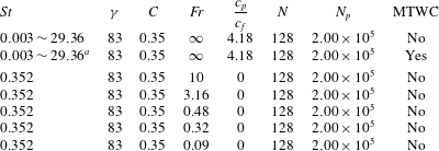
Tables 1 and 2 give the parameters of the different simulations performed. In a first set of simulations, we consider the effect of varying the Stokes number of the particles neglecting their thermal inertia, direct feedback on the fluid momentum and gravitational settling. As seen in table 1, different values of
 $\unicode[STIX]{x1D6FE}$
(at constant
 $C$
) and different values of
 $C$
(at constant
 $\unicode[STIX]{x1D6FE}$
) are considered. The sets of simulations presented in table 2 were carried out to analyse the influence of the particle thermal inertia, momentum two-way coupling, as well as the effect of the particle settling. Note that for all simulations presented in tables 1 and 2, we set
 $Pr=1$
. As seen in the tables, the mesh resolution
 $\unicode[STIX]{x1D6E5}/\ell _{\ast }=\unicode[STIX]{x1D6FE}/N$
ranges from 0.55 to 0.75 which is enough to resolve the dissipative scale.
As in Zamansky et al. (Reference Zamansky, Coletti, Massot and Mani2014), all the simulations are initialized with randomly distributed particles and with zero velocity and temperature fluctuations for both fluid and particles. After a transient state, the flow reaches a statistically steady state which is our interest in this paper.
Parameters of the different simulations with zero particle thermal inertia and settling velocity.
 $N$
is the size of the mesh in each direction,
 $N_{p}$
is the number of particles.
 $St=0.003\sim 29.36$
refers to
 $St=0.003$
, 0.019, 0.074, 0.352, 1.064, 7.343 and 29.36, and MTWC indicates if the momentum two-way coupling
 $f$
is taken into account in (2.2).

Parameters of the different simulations for finite particle thermal inertia and settling velocity. For details see the caption of table 1. Here
 $0.003\sim 29.36^{a}$
refers to
 $St=0.003$
, 0.019, 0.074, 0.352, 1.064, 4.26, 7.343, 12.69 and 29.36. Additionally for all simulations
 $\unicode[STIX]{x1D70C}_{p}/\unicode[STIX]{x1D70C}_{0}=909$
.

4 Results and discussion for particles with zero thermal inertia and zero settling velocity
In order to reduce the parameter space and to focus on the bulk of the interplay mechanisms, we first consider non-settling particles in thermal equilibrium with the surrounding fluid (
 $Fr^{-1}\rightarrow 0$
and
 $c_{p}/c_{f}\rightarrow 0$
, table 1). Although the settling velocity is neglected, gravity is retained in the buoyancy forcing. This approximation bears relevance to particles which are still inertial but possess limited fall speed, while allowing a significantly simplified analysis. Moreover, as will be shown in § 5.2, the cases with finite settling velocity with
 $Fr>1$
quickly approximate the limit behaviour at
 $Fr=\infty$
. In the present section we are also assuming that the mass fraction of the disperse phase is everywhere small, and so we neglect the interphase momentum exchange in (2.9). In § 5.1 this assumption is relaxed along with considering a finite value of
 $c_{p}/c_{f}$
in order to assess the influence of these simplifications on the studied flow.
4.1 Clustering transition
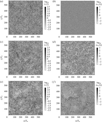
In figure 1 we present visualizations of the instantaneous particle concentration field and fluid temperature fluctuations
 $\unicode[STIX]{x1D703}$
in a vertical plane for three levels of particle inertia:
 $St=0.003$
,
 $St=0.352$
and
 $St=7.343$
. In this figure the concentration is normalized by the average particle concentration
 $\overline{n}$
and
 $\unicode[STIX]{x1D703}$
is normalized by
 $\overline{\unicode[STIX]{x1D703}^{2}}^{1/2}$
. It is observed that for the smallest particle inertia, both fields are fairly homogeneous with only small-scale patterns in the temperature field. At the intermediate Stokes number, highly concentrated clusters of particles appear along with a more coherent distribution the temperature field organized in sheet-like structures. It can be visually checked that, for this Stokes number, the largest temperature fluctuations are highly correlated with the high particle concentration spots. This is in agreement with the conclusions drawn previously in Zamansky et al. (Reference Zamansky, Coletti, Massot and Mani2014). For the high Stokes number, the particles distribution becomes again much more homogeneous although very large areas, commensurate with the size of the overall domain, depleted of particles subsist. The temperature field also present large regions of positive and negative fluctuations with typical mixing layer structures in between.
Visualization in a
 $x{-}z$
plane: (a,c,e) of the logarithm of the particle concentration field (as computed by (3.1)) normalized by the mean concentration
 $n/\overline{n}$
, and (b,d,f) the fluid temperature fluctuations normalized by its standard deviation
 $\unicode[STIX]{x1D703}/\overline{\unicode[STIX]{x1D703}^{2}}^{1/2}$
. For
 $\unicode[STIX]{x1D6FE}=570$
and
 $C=0.19$
, at three Stokes numbers:
 $St=0.003$
(a,b),
 $St=0.352$
(c,d) and
 $St=7.343$
(e,f).

Figure 2 depicts the structure of the turbulent kinetic energy dissipation rate
 $\unicode[STIX]{x1D700}$
and of the scalar dissipation rate
 $\unicode[STIX]{x1D700}_{\unicode[STIX]{x1D703}}$
, for the same snapshots as in figure 1. Both quantities are normalized by their respective mean values. The effect of the Stokes number on the spatial organization of the turbulence dissipation rate is not very pronounced. Filaments of intense dissipation are observed for the three particle inertia, although for the two largest Stokes numbers the filaments appear to be more intense and corrugated. The temperature dissipation rate is fairly homogeneous for the smallest particle inertia. No structures are seen and only small deviations from the mean value are observed. At
 $St=0.352$
and
 $St=7.343$
instead, the temperature dissipation rate presents filaments of very high intensity (more than two decades larger than the mean values, as will be confirmed in figure 18). By comparing with the temperature fields in figure 1 we observe, as expected, that the filaments are found where the temperature gradient is large.
Visualization in a
 $x{-}z$
plane: (a,c,e) logarithm of the turbulent kinetic energy dissipation rate normalized by its mean value
 $\log _{10}(\unicode[STIX]{x1D700}/\overline{\unicode[STIX]{x1D700}})$
and (b,d,f) logarithm of the temperature fluctuation dissipation rate normalized by its mean value
 $\log _{10}(\unicode[STIX]{x1D700}_{\unicode[STIX]{x1D703}}/\overline{\unicode[STIX]{x1D700}_{\unicode[STIX]{x1D703}}})$
. For
 $\unicode[STIX]{x1D6FE}=570$
and
 $C=0.19$
, at three Stokes numbers:
 $St=0.003$
(a,b),
 $St=0.352$
(c,d) and
 $St=7.343$
(e,f).

We now investigate the effect of the Stokes number, the non-dimensional particle number density,
 $C$
and the non-dimensional box size,
 $\unicode[STIX]{x1D6FE}$
, on average quantities characterizing the flow. In figures 3 and 4 we consider the mean turbulent kinetic energy, mean dissipation rate of turbulent kinetic energy, fluid temperature variance and mean rate of dissipation of the temperature fluctuations. It is important to note that in these figures all the quantities are normalized by
 $\ell _{\ast }$
,
 $t_{\ast }$
and
 $\unicode[STIX]{x1D703}_{\ast }$
. Those scales being independent of
 $St$
,
 $C$
and
 $\unicode[STIX]{x1D6FE}$
, it is straightforward to discuss the effect of those parameters.
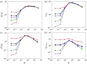
First we focus in figure 3 on the effect of both Stokes number and mean particle concentration. All quantities appear to peak around
 $St=1$
, independently of the concentration. For small Stokes numbers, the statistics are dependent on the overall particle number density while, above
 $St\approx 0.1$
, this dependency vanishes in most cases (the dependency of
 $\overline{\unicode[STIX]{x1D700}_{\unicode[STIX]{x1D703}}}$
on the concentration is attributed to the small number of particles in the system for
 $C=0.035$
and
 $C=0.19$
).
The influence of the mean particle concentration at low Stokes numbers reflects that the mean inter-particle distance is an important length scale, and that the dynamics is essentially driven by the thermal plumes issued from individual particles. Conversely, for high enough Stokes numbers, the dynamics is not governed by individual particle effects but by particle clustering.
Influence of Stokes number and the mean particle concentration on the turbulent kinetic energy (a), the dissipation rate of turbulent kinetic energy (b), the fluid temperature variance (c), and the mean dissipation rate of temperature fluctuations (d) normalized respectively by
 $u_{\ast }=\ell _{\ast }/t_{\ast }$
,
 $\unicode[STIX]{x1D700}_{\ast }=\ell _{\ast }^{2}t_{\ast }^{-3}$
,
 $\unicode[STIX]{x1D703}_{\ast }=\unicode[STIX]{x1D6FD}t_{\ast }$
and
 $\unicode[STIX]{x1D700}_{\unicode[STIX]{x1D703},\ast }=\unicode[STIX]{x1D703}_{\ast }^{2}t_{\ast }^{-1}$
, in log–log scales. For
 $\unicode[STIX]{x1D6FE}=83$
and
 $C=0.035$
(red triangles), 0.19 (black squares), 0.35 (blue circles), 1.82 (green squares), and 8.77 (purple stars).

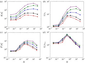
Figure 4 shows the effect of the Stokes number on the various statistics for five non-dimensionalized box sizes,
 $\unicode[STIX]{x1D6FE}$
. We observe a maximum at a Stokes number which shifts to higher values when
 $\unicode[STIX]{x1D6FE}$
is increased, but is in general of order 1. At vanishingly small Stokes numbers, the averaged quantities are practically independent of
 $\unicode[STIX]{x1D6FE}$
, except for the turbulent kinetic energy. When the Stokes number is increased, the influence of
 $\unicode[STIX]{x1D6FE}$
is significant and indicates an increase in both velocity and temperature fluctuations with the increasing domain size. This is consistent with the picture of a cluster-dominated system, in which the clusters present wide range of size along with regions depleted in particles of dimensions commensurate with the large scales of the flow. Interestingly though, the domain size has no sizable effect on the mean temperature dissipation rate. Since
 $\overline{\unicode[STIX]{x1D700}_{\unicode[STIX]{x1D703}}}$
is also roughly independent of the particle concentration, for sufficiently large Stokes number (figure 3), it appears to be only dependent on
 $St$
when the particles organize in clusters. This has important consequences for the model linking the temperature dissipation rate to the local particle clustering, which we present in the next section.
Influence of Stokes number and the non-dimensional box size
 $\unicode[STIX]{x1D6FE}$
on the turbulent kinetic energy (a), the dissipation rate of turbulent kinetic energy (b), the fluid temperature variance (c), and the mean dissipation rate of temperature fluctuations (d) normalized respectively by
 $u_{\ast }=\ell _{\ast }/t_{\ast }$
,
 $\unicode[STIX]{x1D700}_{\ast }=\ell _{\ast }^{2}t_{\ast }^{-3}$
,
 $\unicode[STIX]{x1D703}_{\ast }=\unicode[STIX]{x1D6FD}t_{\ast }$
and
 $\unicode[STIX]{x1D700}_{\unicode[STIX]{x1D703},\ast }=\unicode[STIX]{x1D703}_{\ast }^{2}t_{\ast }^{-1}$
, in log–log scales. For
 $C=0.19$
and
 $\unicode[STIX]{x1D6FE}=48$
(red triangles), 83 (black squares), 190 (blue circles), 330 (green squares) and 570 (purple stars).

Although the usual definitions of turbulent scales rely on the concept of inertial range, which is not necessarily the case here as discussed in § 4.3, to discuss the turbulent nature of this flow, we provide estimation of the Reynolds number based on the Taylor scale
 $R_{\unicode[STIX]{x1D706}}=\sqrt{\overline{{u^{\prime }}^{2}}}\unicode[STIX]{x1D706}/\unicode[STIX]{x1D708}$
. Using the classical estimation of the Taylor scale,
 $\unicode[STIX]{x1D706}=\sqrt{15\overline{{u^{\prime }}^{2}}\unicode[STIX]{x1D708}/\overline{\unicode[STIX]{x1D700}}}$
, with the characteristic velocity estimated from the turbulent kinetic energy,
 $\overline{{u^{\prime }}^{2}}\approx 2/3K$
, one obtains the following relation for the Reynolds number based on the Taylor scale:
 $R_{\unicode[STIX]{x1D706}}=(2/3)\sqrt{15}(K/u_{\ast }^{2})(\overline{\unicode[STIX]{x1D700}}/\unicode[STIX]{x1D700}_{\ast })^{-1/2}$
. Depending on the parameters,
 $R_{\unicode[STIX]{x1D706}}$
ranges from 15 (
 $\unicode[STIX]{x1D6FE}=83$
,
 $C=8.77$
,
 $St=0.003$
) to 250 (
 $\unicode[STIX]{x1D6FE}=570$
,
 $C=0.19$
,
 $St=1.064$
) as can be computed from figures 3 and 4. Similarly, the usual Stokes number based on the Kolmogorov time scale,
 $St_{\unicode[STIX]{x1D702}}=\unicode[STIX]{x1D70F}_{p}/\unicode[STIX]{x1D70F}_{\unicode[STIX]{x1D702}}$
, can be deduced from the value of
 $\overline{\unicode[STIX]{x1D700}}/\unicode[STIX]{x1D700}_{\ast }$
:
 $St_{\unicode[STIX]{x1D702}}=St(\overline{\unicode[STIX]{x1D700}}/\unicode[STIX]{x1D700}_{\ast })^{1/2}$
.
4.2 Scaling
Similarly to Hinch (Reference Hinch, Guyon, Nadal and Pomeau1988), Brenner (Reference Brenner1999) and Aliseda et al. (Reference Aliseda, Cartellier, Hainaux and Lasheras2002), we consider both thermal and momentum budgets on a volume of fluid containing a cluster of particles in order to represent the active source of heat and buoyancy. Such volumes of fluid are denoted below as ‘effective particles’. The thermal budget of such an effective particle is written as:
 $$\begin{eqnarray}\unicode[STIX]{x1D70C}_{0}c_{f}V_{c}\frac{\text{d}}{\text{d}t}\unicode[STIX]{x1D703}_{c}=N_{p,c}\unicode[STIX]{x1D6F7}_{p}-\unicode[STIX]{x1D70C}_{0}c_{f}V_{c}\frac{\unicode[STIX]{x1D703}_{c}}{\unicode[STIX]{x1D70F}_{\unicode[STIX]{x1D703},c}},\end{eqnarray}$$
where
 $V_{c}$
is the characteristic volume of the
 $c^{th}$
cluster,
 $N_{p,c}$
is the number of actual particles contained in it,
 $\unicode[STIX]{x1D703}_{c}$
is its characteristic temperature and
 $\unicode[STIX]{x1D70F}_{\unicode[STIX]{x1D703},c}$
represents its temperature mixing time. The left-hand side of (4.1) is the cluster thermal inertia (recall that here we neglect the thermal inertia of the individual particles), the first term on the right-hand side accounts for the heat source in it and the second term represents the relaxation to thermal equilibrium with the bulk flow. Note that we assume
 $\overline{\unicode[STIX]{x1D703}}=0$
. i.e. we take the characteristic bulk temperature to be equal to the mean temperature, due to the relatively small particle volume fraction in the cluster. Assuming stationarity, equation (4.1) simplifies to:
 $$\begin{eqnarray}\unicode[STIX]{x1D703}_{c}=\unicode[STIX]{x1D6FD}\frac{N_{p,c}}{V_{c}\overline{n}}\unicode[STIX]{x1D70F}_{\unicode[STIX]{x1D703},c}.\end{eqnarray}$$
The momentum balance for an effective particle reads:
 $$\begin{eqnarray}\unicode[STIX]{x1D70C}_{0}V_{c}\frac{\text{d}}{\text{d}t}u_{c}=\unicode[STIX]{x1D70C}_{0}V_{c}\unicode[STIX]{x1D6FC}g\unicode[STIX]{x1D703}_{c}-\unicode[STIX]{x1D70C}_{0}V_{c}\frac{u_{c}}{\unicode[STIX]{x1D70F}_{c}},\end{eqnarray}$$
where
 $u_{c}$
is the velocity of the effective particle and
 $\unicode[STIX]{x1D70F}_{c}$
is its momentum relaxation time. Notice that the linearized state equation has been used to express the buoyancy term:
 $g(1-\unicode[STIX]{x1D70C}_{0}/\unicode[STIX]{x1D70C}_{c})=\unicode[STIX]{x1D6FC}g\unicode[STIX]{x1D703}_{c}$
. In case of stationarity one obtains:
 $$\begin{eqnarray}u_{c}=\unicode[STIX]{x1D6FC}g\unicode[STIX]{x1D703}_{c}\unicode[STIX]{x1D70F}_{c}.\end{eqnarray}$$
Evolution of statistical quantities with the non-dimensional mean particle concentration
 $C=\overline{n}\ell _{\ast }^{3}$
for different Stokes numbers, and
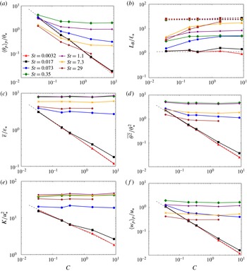
 $\unicode[STIX]{x1D6FE}=83$
. Plots are in log–log scales. (a) the mean particle temperature and comparison with the curve
 $0.13~C^{-1}$
(dashed lines); (b) the Bolgiano length scale, and the velocity integral length scale in dashed lines; (c) the mean dissipation rate normalized by
 $\unicode[STIX]{x1D700}_{\ast }=\ell _{\ast }^{2}t_{\ast }^{-3}$
and comparison with the curve
 $0.43~C^{-3/5}$
(dashed lines); (d) the fluid temperature variance and comparison with the curve
 $0.2~C^{-4/5}$
(dashed lines); (e) the fluid kinetic energy and comparison with the curve
 $4~C^{-2/5}$
(dashed lines); (f) mean particle vertical velocity and comparison with the curve
 $0.07~C^{-4/5}$
(dashed lines).

4.2.1 Vanishing particle inertia
As seen in figure 1, the particle distribution is almost homogeneous for small Stokes numbers. The absence of actual clusters implies:
 $N_{p,c}=1$
in (4.2), meaning that each effective particle encompasses only one actual particle. According to (2.26) and (2.27), the characteristic length and time scales of the convective cells around each particle are given by
 $\ell _{c}=\ell _{\ast }$
and
 $\unicode[STIX]{x1D70F}_{\unicode[STIX]{x1D703},c}=t_{\ast }$
. In addition, we consider that
 $V_{c}=\ell _{c}^{3}=\ell _{\ast }^{3}$
. Substituting in (4.2) one obtains:
 $$\begin{eqnarray}\langle \unicode[STIX]{x1D703}_{p}\rangle _{p}\sim \unicode[STIX]{x1D703}_{p,0}=\frac{\unicode[STIX]{x1D6FD}t_{\ast }}{\ell _{\ast }^{3}\overline{n}}=\unicode[STIX]{x1D703}_{\ast }C^{-1}.\end{eqnarray}$$
We introduce
 $\unicode[STIX]{x1D703}_{p,0}$
, which denotes the characteristics particle temperature in the small Stokes number limit. Equation (4.5) is tested in figure 5(a). It is observed that for the two smallest Stokes numbers (
 $St=0.0029$
and
 $0.017$
), the mean particle temperature follows well the relation (4.5) over all the range of particle concentrations considered. Conversely, when the Stokes number is increased, the mean particle temperature deviates significantly from (4.5): for large particle concentrations. It reaches a value independent of concentration but dependent on the Stokes number (as also observed in figure 3). At low concentrations, the particle mean temperature at large
 $St$
appears to approach asymptotically (4.5). This is a consequence of the small number of particles: even when the Stokes number is not small, the particles in the system are not numerous enough to form clusters and their individual dynamics dominates.
The scaling proposed here assumes no collective particle effects, and this is valid either for vanishingly small particle inertia or small number of particles. To specify this limit, let us introduce the following time scale from (4.5):
 $$\begin{eqnarray}t_{0}=t_{\ast }C^{-1}\sim \frac{\langle \unicode[STIX]{x1D703}_{p}\rangle _{p}}{\unicode[STIX]{x1D6FD}}.\end{eqnarray}$$
This time scale is related to the characteristic heating rate of the particles in the absence of collective effects. The vanishing particle inertia limit corresponds to:
 $$\begin{eqnarray}\frac{\unicode[STIX]{x1D70F}_{p}}{t_{0}}=St\cdot C=St_{0}\rightarrow 0.\end{eqnarray}$$
We notice that a necessary condition to describe the particle temperature from (4.5) is the absence of large fluctuations in the particle temperature. This will be confirmed later in figure 18 where the p.d.f. of the particle temperature is shown. From this figure we see that at small Stokes number the particles temperature presents nearly Gaussian fluctuations.
We now develop further this argument to propose a power-law dependency on
 $C$
for other statistical quantities of interest. From the thermal balance equation in the bulk of the fluid, equation (2.22), one obtains the scaling for the mean thermal dissipation rate:
 $$\begin{eqnarray}\overline{\unicode[STIX]{x1D700}_{\unicode[STIX]{x1D703}}}\sim \unicode[STIX]{x1D700}_{\unicode[STIX]{x1D703},0}=\unicode[STIX]{x1D6FD}\unicode[STIX]{x1D703}_{\ast }C^{-1}.\end{eqnarray}$$
Assuming that the Bolgiano scale,
 $L_{B}=\overline{\unicode[STIX]{x1D700}}^{5/4}\unicode[STIX]{x1D700}_{\unicode[STIX]{x1D703}}^{-3/4}(\unicode[STIX]{x1D6FC}g)^{-3/2}$
(typically used in turbulent thermal convection), is of the order of the dissipative scale
 $L_{B}=\ell _{\ast }$
, that is to say there is no inertial range (Lohse & Xia Reference Lohse and Xia2009), one gets the following scaling for the mean dissipation rate:
 $$\begin{eqnarray}\overline{\unicode[STIX]{x1D700}}\sim \unicode[STIX]{x1D700}_{0}=\ell _{\ast }^{2}t_{\ast }^{-3}C^{-3/5}.\end{eqnarray}$$
The validity of the relation (4.9) along with assumption
 $L_{B}=\ell _{\ast }$
for
 $St\ll 1$
is assessed in figures 5(b,c). Very good agreement is clearly observed.
From the Bolgiano–Obukhov scaling argument for the temperature,
 $\overline{(\unicode[STIX]{x1D703}(\boldsymbol{x}\,+\,\boldsymbol{r})\!-\unicode[STIX]{x1D703}(\boldsymbol{x}))^{2}}=\overline{\unicode[STIX]{x1D700}}_{\unicode[STIX]{x1D703}}^{4/5}(\unicode[STIX]{x1D6FC}g)^{-2/5}r^{2/5}$
(Bolgiano Reference Bolgiano1959; Obukhov Reference Obukhov1959; Lohse & Xia Reference Lohse and Xia2009), we obtain the estimation of the fluid temperature variance, assuming that the integral length scale of the temperature fluctuation is proportional to
 $\ell _{\ast }$
(as shown in figure 5
b):
 $$\begin{eqnarray}\overline{\unicode[STIX]{x1D703}^{2}}\sim \unicode[STIX]{x1D703}_{0}^{2}=\unicode[STIX]{x1D703}_{\ast }^{2}C^{-4/5}.\end{eqnarray}$$
Moreover we observe that the variance of the particle temperature is proportional to the fluid temperature variance (not shown). Similarly the Bolgiano–Obukhov scaling for the velocity,
 $\overline{(\boldsymbol{u}(\boldsymbol{x}+\boldsymbol{r})-\boldsymbol{u}(\boldsymbol{x}))^{2}}=\overline{\unicode[STIX]{x1D700}}_{\unicode[STIX]{x1D703}}^{2/5}(\unicode[STIX]{x1D6FC}g)^{4/5}r^{6/5}$
, gives an estimate of the velocity variance:
 $$\begin{eqnarray}K\sim K_{0}=u_{\ast }^{2}C^{-2/5}.\end{eqnarray}$$
Finally, the mean vertical particle velocity is estimated from the momentum budget for an effective particle. In (4.4) the relaxation time scale is estimated via an eddy viscosity assumption:
 $\unicode[STIX]{x1D70F}_{c}=\ell _{c}/u^{\prime }=\ell _{c}K^{-1/2}$
. Then with the previous relations we get:
 $$\begin{eqnarray}\langle w_{p}\rangle _{p}\sim u_{\ast }C^{-4/5}.\end{eqnarray}$$
Figures 5(d–f), compare relations (4.10), (4.11) and (4.12) with the numerical simulations. Again, a very good agreement is observed for the smaller Stokes number. The deviation observed at
 $St=0.017$
for large particle concentration is interpreted in view of (4.7): when the particle concentration becomes large, we expect a departure from the individual particle limit. We also note that the proportionality in (4.5)–(4.12), as determined by a linear fit, are of order 1 for all the cases (see caption of figure 5).
4.2.2 Cluster-driven dynamics for intermediate particle inertia
When the Stokes number increases, the particle distribution becomes non-homogeneous. The resulting clusters present a wide range of scales, as illustrated in figure 1. More qualitatively, we provide in figure 6 the radial distribution function (Sundaram & Collins Reference Sundaram and Collins1997) for the various Stokes numbers and for
 $\unicode[STIX]{x1D6FE}=570$
and
 $C=0.19$
. The radial distribution function is defined as the ratio of the number of particle pairs at a given separation
 $r$
to the expected number of particle pairs for uniformly distributed particles. For vanishingly small Stokes number there is no sign of clustering, while we observe a maximum clustering for
 $St=0.35$
. At the largest Stokes numbers there is only large-scale clustering. One can clearly see that at small distances the radial distribution function presents power laws whose exponent is very dependent on the
 $St$
number. Figure 7 shows the correlation dimension defined as
 ${\mathcal{D}}=3+a$
,
 $a$
being the exponent of the power law obtained by fitting the pair correlation function at small distances (
 $r/\ell _{\ast }<4$
). The correlation dimension is plotted against the Stokes number for the various values of
 $\unicode[STIX]{x1D6FE}$
and
 $C$
considered in the paper. We observe that the small-scale clustering is independent of
 $C$
and is only weakly dependent of
 $\unicode[STIX]{x1D6FE}$
.
Radial distribution function (RDF) for the various Stokes numbers (
 $St=0.003$
, 0.019, 0.074, 0.352, 1.064, 7.343 and 29.36, from light grey to black respectively) at
 $\unicode[STIX]{x1D6FE}=570$
,
 $C=0.19$
. Comparison with the power law obtained by fit of the DNS in dashed lines.

Evolution with Stokes number of the correlation dimension. (a) For
 $\unicode[STIX]{x1D6FE}=83$
and
 $C=0.035$
(red triangles), 0.19 (black squares), 0.35 (blue circles), 1.82 (green squares), 8.77 (purple stars). (b) For
 $C=0.19$
and
 $\unicode[STIX]{x1D6FE}=48$
(red triangles), 83 (black squares), 190 (blue circles) and 330 (green squares).

As a consequence of the particle clustering, in (4.2) and (4.4) the parameters describing the effective particle, such as
 $V_{c}$
,
 $N_{p,c}$
,
 $\unicode[STIX]{x1D703}_{c}$
,
 $u_{c}$
are a priori random variables. The model equation (4.2) is re-expressed as:
 $$\begin{eqnarray}\unicode[STIX]{x1D703}_{c}=\unicode[STIX]{x1D6FD}\frac{n_{c}}{\overline{n}}\unicode[STIX]{x1D70F}_{\unicode[STIX]{x1D703},c},\end{eqnarray}$$
where we introduce
 $n_{c}=N_{p,c}/V_{c}$
the number density of actual particles within an effective particle. In this regime the effective particles correspond to particle clusters, which we shall now characterize.
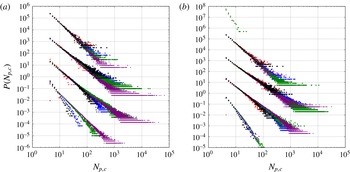
As proposed by Monchaux, Bourgoin & Cartellier (Reference Monchaux, Bourgoin and Cartellier2010), we detect particle clusters using the Voronoï tessellation of the particle positions. As shown by Zamansky et al. (Reference Zamansky, Coletti, Massot and Mani2014), the p.d.f. of the Voronoï cell volumes present very large tails for intermediate particle inertia. We use the connectivity of the Voronoï tessellation to form sets of particles that define individual clusters (details of the algorithm are given in appendix B). Once the clusters are identified, it is possible to compute their statistical features. In figure 8 we present the p.d.f. of the number of particles per cluster. This p.d.f. exhibits power-law behaviour over a few decades, with a slope depending on the Stokes number but independent of concentration or box size. Clusters with a very large number of particles are observed. For example, at Stokes
 $St=1.064$
, the largest cluster includes almost 10 % of the particles of the system.
P.d.f. of the number of particles per cluster. For
 $St=0.074$
, 0.352, 1.064 and 7.343 respectively shifted upward by two decades each. (a) For
 $\unicode[STIX]{x1D6FE}=83$
and
 $C=0.035$
(red triangles),
 $0.19$
(black squares),
 $0.35$
(blue circles),
 $1.82$
(green squares),
 $8.77$
(purple stars). (b) For
 $C=0.19$
and
 $\unicode[STIX]{x1D6FE}=48$
(red triangles),
 $83$
(black squares),
 $190$
(blue circles),
 $330$
(green squares) and
 $570$
(purple stars).

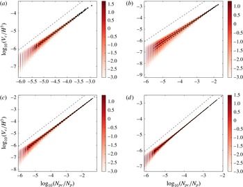
In figure 9 we consider the joint probability of
 $N_{p,c}$
and
 $V_{c}$
in order to estimate the particle concentration in clusters
 $n_{c}=N_{p,c}/V_{c}$
, which is an unknown in (4.13). The cluster volume is estimated as the sum of the volume of the Voronoï cells of the particles belonging to the cluster. The particle number and cluster volumes are normalized by the total number of particles and the total domain volume, respectively. In this figure we present the plot for
 $\unicode[STIX]{x1D6FE}=83$
and
 $C=8.77$
and for
 $St=0.074$
, 0.352, 1.064 and 7.343. We observe that the cluster volumes and the numbers of particles per cluster are highly and linearly correlated. Moreover, we observe that the correlation between the cluster volume and its number of particles is much more pronounced for large clusters. As a consequence, one can conclude that the particle concentration in large clusters is almost deterministic, and neglecting the small fluctuations one can write:
 $\langle \log (V_{c}/H^{3})|\log (N_{p,c}/N_{p})\rangle \sim \log (\widetilde{V_{c}}(N_{p,c}/N_{p})/H^{3})$
, where
 $\widetilde{V_{c}}(N_{p,c}/N_{p})$
denotes for the characteristic volume of clusters with
 $N_{p,c}$
particles inside. Moreover, from the linear behaviour of the conditional average, we have:
 $\log (\widetilde{V_{c}}(N_{p,c}/N_{p})/H^{3})=A\log (N_{p,c}/N_{p})+B$
. This relation transforms to:
 $$\begin{eqnarray}\frac{n_{c}}{\overline{n}}=\left(\frac{\widetilde{V_{c}}(N_{p,c})}{H^{3}}\right)^{(1-A)/A}\,e^{-B/A}.\end{eqnarray}$$
The coefficients
 $A$
and
 $B$
in (4.14) are a priori dependent on the parameters of the flows (
 $St$
,
 $\unicode[STIX]{x1D6FE}$
and
 $C$
). They are estimated by linear fitting for the various DNS. We find that
 $A=1$
with a precision of at least
 $\pm 10^{-4}$
for every case considered in table 1. As a consequence, for sufficiently large clusters, the particle concentration in the clusters is independent (on average) of the cluster size, and (4.14) reduces to:
 $$\begin{eqnarray}\frac{n_{c}}{\overline{n}}=e^{-B}.\end{eqnarray}$$
The particle concentration in large clusters, as obtained from the measure of the
 $B$
coefficient through (4.15), is given for the various parameters considered by the DNS in figure 10. From this figure we observe that the particle concentration in clusters presents a peak around
 $St=0.35$
, where it is approximately ten times the mean concentration. Remarkably
 $n_{c}$
is almost independent of both
 $\unicode[STIX]{x1D6FE}$
and
 $C$
(the reduced values observed for
 $C=0.035$
are likely due to the small number of particles in the domain). Therefore, assuming that
 $\unicode[STIX]{x1D70F}_{\unicode[STIX]{x1D703},c}$
in model (4.13) is not dependent of the particle concentration, the characteristic temperature of large clusters is essentially a function of the Stokes number only. And since the large clusters gather most of the particles (as seen in figures 8 and 9) we estimate as well that the mean particle temperature presents a behaviour similar to
 $n_{c}$
. As a consequence, the mean temperature dissipation rate, which is linearly related to the mean particle temperature through (2.22), should also depend only on the Stokes number. This is in agreement with the trends in figures 3 and 4 which showed, for intermediate particle inertia, almost no dependency of temperature dissipation rate on
 $C$
and
 $\unicode[STIX]{x1D6FE}$
. Therefore in this regime the dynamics of the flow appears to be governed by the formation of self-similar clusters, the features of which are mostly dictated by the particle Stokes number. Similarly, we can conclude that the other statistical quantities of the flow become independent of the mean particle concentration when the dynamics of the flow leads to the formation of self-similar clusters of particles.
Colour map for the logarithm of the joint probability density function of the logarithm of the number of particles per cluster
 $N_{p,c}$
and the cluster volumes
 $V_{c}$
for four Stokes numbers,
 $St=0.074$
(a), 0.352 (b), 1.064 (c) and 7.343 (d) at
 $\unicode[STIX]{x1D6FE}=83$
and
 $C=8.77$
. The number of particles is normalized by the total number of particles in the system, and the cluster volume is normalized by the total volume. The solid line is the conditional average of the cluster volumes with the number of particles per cluster:
 $\langle \log _{10}(V_{c}/H^{3})|\log _{10}(N_{p,c}/N_{p})\rangle$
and black dashed lines is the conditional average plus or minus the conditional standard deviation, with the standard deviation defined as follows:
 $(\langle \log _{10}(V_{c}/H^{3})|\log _{10}(N_{p,c}/N_{p})^{2}\rangle -\langle \log _{10}(V_{c}/H^{3})|\log _{10}(N_{p,c}/N_{p})\rangle ^{2})^{1/2}$
. The grey dashed lines corresponds to the bisectrix
 $\log _{10}(V_{c}/H^{3})=\log _{10}(N_{p,c}/N_{p})$
.

Mean particle concentration in large clusters as a function of the Stokes number. (a) For
 $\unicode[STIX]{x1D6FE}=83$
and
 $C=0.035$
(red triangles),
 $0.19$
(black squares),
 $0.35$
(blue circles),
 $1.82$
(green squares),
 $8.77$
(purple stars); (b) for
 $C=0.19$
and
 $\unicode[STIX]{x1D6FE}=48$
(red triangles),
 $83$
(black squares),
 $190$
(blue circles),
 $330$
(green squares) and
 $570$
(purple stars).

As discussed above, we observe evidence of a clustering transition with increasing the Stokes number. Based on this observation, we now discuss the dependency on the Stokes number at intermediate particle inertia. By analogy with the continuous phase transitions, we expect that the order parameters, for instance the cluster concentration
 $n_{c}$
or the particle mean temperature, are continuous across the transition, while their first derivatives against the control parameter (here the Stokes number) present singular behaviour at the transition. This leads us to assume the following functional shape, reminiscent of systems close to a critical point, for various macroscopic quantities such as
 $K$
,
 $\overline{\unicode[STIX]{x1D700}}$
,
 $\overline{\unicode[STIX]{x1D703}^{2}}$
and
 $\overline{\unicode[STIX]{x1D700}_{\unicode[STIX]{x1D703}}}$
denoted generically by
 $\unicode[STIX]{x1D712}$
:
 $$\begin{eqnarray}\frac{\unicode[STIX]{x1D712}-\unicode[STIX]{x1D712}_{0}}{\unicode[STIX]{x1D712}_{0}}=D_{\unicode[STIX]{x1D712}}(\unicode[STIX]{x1D6FE})(St_{0}-St_{0,crit})^{d_{\unicode[STIX]{x1D712}}},\end{eqnarray}$$
with
 $St_{0}=St\cdot C$
as already defined in (4.7) and
 $St_{0,crit}$
the critical Stokes number above which the clustering transition occurs.
 $\unicode[STIX]{x1D712}_{0}$
is the characteristic scale of
 $\unicode[STIX]{x1D712}$
before the transition, i.e. in the small particle inertia limit, as given by (4.5)–(4.12). The value of the exponent
 $d_{\unicode[STIX]{x1D712}}$
and the expression of
 $D_{\unicode[STIX]{x1D712}}(\unicode[STIX]{x1D6FE})$
, which account for the box size effect, are dependent on the quantity
 $\unicode[STIX]{x1D712}$
considered. A priori
 $St_{0,crit}$
,
 $D_{\unicode[STIX]{x1D712}}$
and
 $d_{\unicode[STIX]{x1D712}}$
are unknown.
The exponent
 $d_{\unicode[STIX]{x1D712}}$
is determined as follows. For
 $St_{0}\gg St_{0,crit}$
, (but maintaining a particle inertia small enough to observe clusters) equation (4.16) approximatively reduces to:
 $$\begin{eqnarray}\frac{\unicode[STIX]{x1D712}}{\unicode[STIX]{x1D712}_{\ast }}\approx \frac{\unicode[STIX]{x1D712}_{0}}{\unicode[STIX]{x1D712}_{\ast }}D(\unicode[STIX]{x1D6FE})C^{d_{\unicode[STIX]{x1D712}}}St^{d_{\unicode[STIX]{x1D712}}},\end{eqnarray}$$
where
 $\unicode[STIX]{x1D712}_{\ast }$
is given by the appropriate combination of
 $\ell _{\ast }$
,
 $t_{\ast }$
and
 $\unicode[STIX]{x1D703}_{\ast }$
. Substituting by the expression for
 $\unicode[STIX]{x1D712}_{0}$
obtained in one of (4.5)-(4.12):
 $\unicode[STIX]{x1D712}_{0}/\unicode[STIX]{x1D712}_{\ast }=A_{\unicode[STIX]{x1D712}}C^{-a_{\unicode[STIX]{x1D712}}}$
, one gets:
 $$\begin{eqnarray}\frac{\unicode[STIX]{x1D712}}{\unicode[STIX]{x1D712}_{\ast }}\approx A_{\unicode[STIX]{x1D712}}D(\unicode[STIX]{x1D6FE})\,C^{d_{\unicode[STIX]{x1D712}}-a_{\unicode[STIX]{x1D712}}}St^{d_{\unicode[STIX]{x1D712}}}.\end{eqnarray}$$
From figure 3 we concluded that the dependency on the concentration vanished for sufficiently large Stokes number. This implies that
 $d_{\unicode[STIX]{x1D712}}=a_{\unicode[STIX]{x1D712}}$
in (4.16). Namely, we obtain for
 $K$
,
 $\overline{\unicode[STIX]{x1D700}}$
,
 $\overline{\unicode[STIX]{x1D703}^{2}}$
and
 $\overline{\unicode[STIX]{x1D700}_{\unicode[STIX]{x1D703}}}$
respectively:
 $d_{K}=2/5$
,
 $d_{\unicode[STIX]{x1D700}}=3/5$
,
 $d_{\unicode[STIX]{x1D703}^{2}}=4/5$
and
 $d_{\unicode[STIX]{x1D700}_{\unicode[STIX]{x1D703}}}=1$
. Notably, this means that
 $\overline{\unicode[STIX]{x1D700}_{\unicode[STIX]{x1D703}}}-\unicode[STIX]{x1D700}_{\unicode[STIX]{x1D703},0}$
increases linearly with
 $St_{0}-St_{0,crit}$
. This is consistent with a maximum segregation argument. According to the resonant eddies assumption of Yoshimoto & Goto (Reference Yoshimoto and Goto2007), the particles are efficiently segregated by the fluid structures having a characteristic time commensurate with the relaxation time of the particle. In the meantime, the particles, being a heat source, impose the time scale of the temperature forcing through their clustering, which evolves on a time scale commensurate with the particle response time. This illustrates the feedback loop mechanism. Note that in § 4.3.1 we study the concentration/temperature and velocity/temperature correlations which also give support to the proposed feedback loop mechanism.
For the critical Stokes number
 $St_{0,crit}$
we propose the estimate
 $St_{0,crit}=0.0035\pm 0.001$
obtained from a fit of the DNS. The value of
 $St_{0,crit}$
does not seem to depend strongly on the non-dimensional parameters, but further studies are required to determine precisely the value of the threshold as well as its dependence on the non-dimensional parameters.
We assume that
 $D_{\unicode[STIX]{x1D712}}(\unicode[STIX]{x1D6FE})$
is a power law of
 $\unicode[STIX]{x1D6FE}$
:
 $D_{\unicode[STIX]{x1D712}}(\unicode[STIX]{x1D6FE})\sim \unicode[STIX]{x1D6FE}^{b_{\unicode[STIX]{x1D712}}}$
. In the next section we discuss the dependency of the flow statistics on the box size for large inertia particles, and as a first estimate we use this value of
 $b_{\unicode[STIX]{x1D712}}$
. Accordingly, one has for
 $K$
,
 $\overline{\unicode[STIX]{x1D703}^{2}}$
,
 $\overline{\unicode[STIX]{x1D700}}$
,
 $\overline{\unicode[STIX]{x1D700}_{\unicode[STIX]{x1D703}}}$
respectively:
 $b_{K}=4/3$
,
 $b_{\unicode[STIX]{x1D703}^{2}}=2/3$
,
 $b_{\unicode[STIX]{x1D700}}=1$
 $b_{\unicode[STIX]{x1D700}_{\unicode[STIX]{x1D703}}}=0$
.
In figure 11 we test the scaling relation (4.16). In this figure
 $(\unicode[STIX]{x1D712}-\unicode[STIX]{x1D712}_{0})/(\unicode[STIX]{x1D712}_{0}\unicode[STIX]{x1D6FE}^{b_{\unicode[STIX]{x1D712}}})$
is plotted versus
 $St_{0}-St_{0,crit}$
in logarithm scales for
 $\unicode[STIX]{x1D712}=K$
,
 $\overline{\unicode[STIX]{x1D700}}$
,
 $\overline{\unicode[STIX]{x1D703}^{2}}$
and
 $\overline{\unicode[STIX]{x1D700}_{\unicode[STIX]{x1D703}}}$
with
 $\unicode[STIX]{x1D712}_{0}$
from (4.5)–(4.11) and
 $b_{\unicode[STIX]{x1D712}}$
given by (4.20)–(4.21). As shown in this figure, for small enough values of
 $St_{0}-St_{0,crit}$
the various quantities present power-law behaviour with a slope in very good agreement with the predicted slope. A confirmation of the critical behaviour of this flow at the clustering transition can be seen in the fact that this scaling law appears to be consistent for all the observables. Moreover, the different curves present a reasonable overlap, justifying the scaling with
 $\unicode[STIX]{x1D6FE}$
.
Plot of
 $(\unicode[STIX]{x1D712}-\unicode[STIX]{x1D712}_{0})/(\unicode[STIX]{x1D712}_{0}D_{\unicode[STIX]{x1D712}}(\unicode[STIX]{x1D6FE}))$
versus
 $St_{0}-St_{0,crit}$
in logarithmic scales and comparison with the power law
 $y=x^{d_{\unicode[STIX]{x1D712}}}$
. With
 $\unicode[STIX]{x1D712}$
denoting the turbulent kinetic energy (a), the mean dissipation rate of turbulent kinetic energy (b), the fluid temperature variance (c) and the mean dissipation rate of temperature fluctuations (d). Open symbols for
 $\unicode[STIX]{x1D6FE}=83$
and
 $C=0.035$
(red triangles),
 $0.19$
(black squares),
 $0.35$
(blue circles),
 $1.82$
(green squares),
 $8.77$
(purple stars); filled symbols for
 $C=0.19$
and
 $\unicode[STIX]{x1D6FE}=48$
(red triangles),
 $83$
(black squares),
 $190$
(blue circles),
 $330$
(green squares) and
 $570$
(purple stars).

4.2.3 Large particle inertia
In this section we propose a scaling law for the statistics of the flow in the case of large particle inertia. We stress that when the particle inertia becomes large, several of the assumptions made at the beginning of § 4 are not strictly valid anymore. First, the particle thermal inertia may not be negligible, and therefore the particle may not be in the thermal equilibrium with the surrounding fluid. Secondly, the particle mass loading becomes important and the momentum two-way coupling with the fluid could become significant. Indeed, in § 5.1 it will be shown that for
 $St>O(1)$
the statistics of the flows are altered when both such effects are accounted for in the simulations. Nevertheless, in this subsection we still remain under those simplifying hypotheses. This scaling is then interpreted as an upper bound for the dependency on
 $\unicode[STIX]{x1D6FE}$
.
When the particle inertia is very large, the particle concentration is nearly homogeneous, as in the vanishing inertia limit (figure 1). The statistics, however, are now almost independent of the mean particle concentration (figure 3). When the particle time scale is larger than the characteristic time
 $t_{H}$
of the buoyancy forcing at the scale of the domain
 $H$
:
 $$\begin{eqnarray}t_{H}=\left(\frac{H}{\unicode[STIX]{x1D6FC}g\unicode[STIX]{x1D6FD}}\right)^{1/3},\end{eqnarray}$$
the particles present uncorrelated ballistic motions. As a consequence, both buoyancy forcing and forcing of the fluid temperature fluctuations take place at the scale of the box. Therefore we have the following estimates:
 $L_{int}\sim H$
and
 $t_{int}\sim t_{H}$
where
 $L_{int}=K^{3/2}/\overline{\unicode[STIX]{x1D700}}$
and
 $t_{int}=K/\overline{\unicode[STIX]{x1D700}}$
are the integral length and time scales. Manipulating the previous relations yields an expression for the characteristic turbulent dissipation rate:
 $$\begin{eqnarray}\unicode[STIX]{x1D700}_{H}=\unicode[STIX]{x1D6FC}g\unicode[STIX]{x1D6FD}\,H,\end{eqnarray}$$
as well as for the characteristic velocity scale:
 $$\begin{eqnarray}u_{H}=(\unicode[STIX]{x1D6FC}g\unicode[STIX]{x1D6FD})^{1/3}H^{2/3}.\end{eqnarray}$$
Similarly, we estimate the characteristic temperature as:
 $$\begin{eqnarray}\unicode[STIX]{x1D703}_{H}=\unicode[STIX]{x1D6FD}t_{H}.\end{eqnarray}$$
The temperature dissipation rate remains set by a balance between the local heat released by the particles and the diffusion process:
 $$\begin{eqnarray}\unicode[STIX]{x1D700}_{\unicode[STIX]{x1D703},H}=\unicode[STIX]{x1D700}_{\unicode[STIX]{x1D703},\ast }=\unicode[STIX]{x1D6FD}^{2}t_{\ast }.\end{eqnarray}$$
In terms of the characteristic scales
 $\ell _{\ast }$
,
 $t_{\ast }$
and
 $\unicode[STIX]{x1D703}_{\ast }$
, introduced in equations (2.25)–(2.27), these relations read:
 $t_{H}=t_{\ast }\unicode[STIX]{x1D6FE}^{1/3}$
,
 $\unicode[STIX]{x1D700}_{H}=\unicode[STIX]{x1D700}_{\ast }\,\unicode[STIX]{x1D6FE}$
,
 $\unicode[STIX]{x1D703}_{H}=\unicode[STIX]{x1D703}_{\ast }\,\unicode[STIX]{x1D6FE}^{1/3}$
and
 $u_{H}=u_{\ast }\,\unicode[STIX]{x1D6FE}^{2/3}$
with
 $\unicode[STIX]{x1D700}_{\ast }=\ell _{\ast }^{2}t_{\ast }^{-3}$
,
 $u_{\ast }=\ell _{\ast }t_{\ast }^{-1}$
.
Turbulent kinetic energy (a), the dissipation rate of turbulent kinetic energy (b), the fluid temperature variance (c) normalized respectively by
 $u_{H}^{2}$
,
 $\unicode[STIX]{x1D700}_{H}$
and
 $\unicode[STIX]{x1D703}_{H}$
plot against
 $St_{H}$
in log–log scales. For
 $C=0.19$
and
 $\unicode[STIX]{x1D6FE}=48$
(red triangles),
 $83$
(black squares),
 $190$
(blue circles),
 $330$
(green squares) and
 $570$
(purple stars).

The previous relations are tested in figure 12, in which the turbulent kinetic energy, the mean turbulence dissipation rate and the fluid temperature variance are normalized by the characteristic scale introduced in (4.20)–(4.22). These quantities are plotted as a function of the Stokes number based on the time scale
 $t_{H}$
(4.19):
 $$\begin{eqnarray}St_{H}=\frac{\unicode[STIX]{x1D70F}_{p}}{t_{H}}=St\,\unicode[STIX]{x1D6FE}^{-1/3}.\end{eqnarray}$$
We observe a good collapse of the curves for the various values of
 $\unicode[STIX]{x1D6FE}$
when the particle inertia becomes large. From this figure it appears that the large inertia limit is reached for
 $St_{H}>1$
, and all quantities peak between
 $St_{H}=0.1$
and 1. Also important is that
 $K$
,
 $\overline{\unicode[STIX]{x1D700}}$
and
 $\overline{\unicode[STIX]{x1D703}}^{2}$
peak for
 $St_{H}=O(1)$
. This is in contrast with the mean temperature dissipation rate which is almost independent of
 $\unicode[STIX]{x1D6FE}$
and which presents a peak at
 $St=O(1)$
regardless of the value of
 $\unicode[STIX]{x1D6FE}$
, as seen in figure 4.
We point out that even for
 $St_{H}<1$
the collapse of the various curves presented in figure 12 is reasonable (although not perfect). This is the reason why we used these power laws with
 $\unicode[STIX]{x1D6FE}$
in the previous paragraph.
Temperature (a), velocity (b) and particle concentration (c) spectra, for the various Stokes numbers (
 $St=0.003$
, 0.019, 0.074, 0.352, 1.064, 7.343 and 29.36, from light grey to black respectively) at
 $\unicode[STIX]{x1D6FE}=570$
,
 $C=0.19$
. Comparison with the power law obtained by fit of the DNS in dashed lines. Insert: exponent of the power law as a function of the Stokes number.

4.3 Spectral analysis
We present the spectral density of the fluid temperature fluctuations, the turbulent kinetic energy and the particle concentration field in figure 13 for
 $\unicode[STIX]{x1D6FE}=570$
and
 $C=0.19$
, which are representative of all domain sizes and concentrations. We consider here the three-dimensional spectra obtained by integration of the Fourier coefficient regardless of the angular dependence. For the temperature fluctuations it reads:
 $E_{\unicode[STIX]{x1D703}}(k)=\int _{|\boldsymbol{k}|=k}\overline{\unicode[STIX]{x1D703}(\boldsymbol{k})\unicode[STIX]{x1D703}^{\ast }(\boldsymbol{k})}\,\text{d}\boldsymbol{k}$
, with
 $\unicode[STIX]{x1D703}^{\ast }(\boldsymbol{k})$
the complex conjugate of
 $\unicode[STIX]{x1D703}(\boldsymbol{k})$
. Also note that here the
 $\overline{\bullet }$
operator stands for the temporal average. In figure 13 the spectra are normalized by the scale introduced in (2.26)–(2.27) and the wavelength
 $k$
is normalized by
 $k_{\ast }=2\unicode[STIX]{x03C0}/\ell _{\ast }$
. A clear power law is present up to wavelengths smaller than
 $0.1k_{\ast }$
regardless of the Stokes number. For higher wavenumbers, an exponential decay characteristic of the dissipative region is observed. The Stokes number has a dramatic effect on the temperature spectra: at very small particle inertia, the power-law exponent is positive, indicating that the structures of the fields are dominated by the small scales. With increasing Stokes number, the power-law exponent at small wavenumber decreases, going through zero at approximately
 $St=0.074$
, and reaching an asymptotic value for the largest particle inertia. The decrease of the power-law exponent with
 $St$
is consistent with the temperature snapshot in figure 1, where we observe that larger structures develop in the temperature field when the Stokes number rises. The evolution of the power-law exponent with the Stokes number is reported in the insert of figure 13. For very small values of the Stokes number, the exponent of the temperature spectra remains constant at approximately
 $+1/3$
. For
 $St$
above the threshold, clusters are formed, and then, when the Stokes number is further increased, the clustering of the system is reinforced. This gradual evolution of the particle clustering cause the smooth evolution the spectra exponent, which decreases down to the ‘Obukhov–Corrsin’ value of
 $-5/3$
obtained for passive scalar fluctuations forced at large scale in isotropic turbulence (Obukhov Reference Obukhov1949; Corrsin Reference Corrsin1951). The continuous evolution of the power-law exponent suggests that it may take non-rational values at intermediate Stokes number. The anomalous values of the exponent are associated with the forcing imposed by the particle clusters, which are seen to have a fractal geometry (as seen in figures 6, 7 and 8). The spectra slope becomes sensitive to the Stokes number from
 $St=0.019$
at
 $C=0.19$
which gives an estimate of
 $St_{0}=0.0036$
consistently with the value proposed for
 $St_{0,crit}$
in § 4.2.2.
Concerning the turbulent velocity spectra, a somewhat similar behaviour is observed, with a continuous decrease of the power-law exponent from approximately
 $-1$
at small Stokes numbers to approximately
 $-5/3$
at large Stokes numbers. The important difference is that the exponent in this case is negative for the entire
 $St$
range, which implies that the integral
 $K=\int _{k_{min}}^{k_{max}}E_{u}(k)\,\text{d}k$
does not converge when increasing the size of the domain (see figure 4). On the other hand, the positive power-law exponent, at small Stokes number, for the temperature spectra implies the convergence of the integral
 $\overline{\unicode[STIX]{x1D703}^{2}}=\int _{k_{min}}^{k_{max}}E_{\unicode[STIX]{x1D703}}(k)\,\text{d}k$
consistent with the independency of the temperature variance on
 $\unicode[STIX]{x1D6FE}$
(see figure 4) at vanishingly small Stokes number.
The spectral density of the particle concentration field characterizes the scale of the concentration fluctuations which is closely related to the particle clustering. As expected, at small Stokes numbers we observe a
 $k^{2}$
power law corresponding to a random homogenous particle distribution. For intermediate Stokes number, one observe an almost flat spectrum, indicating that the particle concentration fluctuates at all scales. At large Stokes numbers, most of the concentration fluctuations take place at very large scales while the smallest scales of the concentration fields become randomly distributed (as shown by the
 $k^{2}$
slope). This evolution of the concentration spectra with
 $St$
appears to be consistent with the findings of the § 4.2.2.
4.3.1 Budget of thermal and kinetic energy
We consider the temperature fluctuations and turbulent kinetic energy budget in spectral space in order to analyse in more detail the original forcing and to provide arguments that the particle clustering imposes the forcing of the flow. Multiplying the Fourier transform of (2.10) by
 $\unicode[STIX]{x1D703}^{\ast }(\boldsymbol{k})$
and taking the average, one obtains the scale by scale temperature budget:
 $$\begin{eqnarray}d_{t}{\textstyle \frac{1}{2}}\overline{|\unicode[STIX]{x1D703}|^{2}(\boldsymbol{k})}=\text{Re}[\overline{\unicode[STIX]{x1D703}^{\ast }(\boldsymbol{k})q^{\prime }(\boldsymbol{k})}]+\text{Re}[\overline{\unicode[STIX]{x1D703}^{\ast }(\boldsymbol{k})N_{\unicode[STIX]{x1D703}}(\boldsymbol{k})}]-\unicode[STIX]{x1D705}k^{2}\overline{|\unicode[STIX]{x1D703}(\boldsymbol{k})|^{2}},\end{eqnarray}$$
where
 $\text{Re}[x]$
denotes the real part of
 $x$
and
 $|\unicode[STIX]{x1D703}(\boldsymbol{k})|^{2}=\unicode[STIX]{x1D703}^{\ast }(\boldsymbol{k})\unicode[STIX]{x1D703}(\boldsymbol{k})$
. The first term on the right-hand side is the averaged source of temperature variance,
 ${\mathcal{P}}_{\unicode[STIX]{x1D703}}(\boldsymbol{k})$
, which is related to the temperature–concentration correlation. The second term represents the inter-scale transfers due to the nonlinear terms,
 $N_{\unicode[STIX]{x1D703}}(\boldsymbol{k})$
being the Fourier transform of the convective term. The last term is the spectral dissipation of the temperature fluctuations,
 ${\mathcal{D}}_{\unicode[STIX]{x1D703}}(\boldsymbol{k})$
. The forcing
 ${\mathcal{P}}_{\unicode[STIX]{x1D703}}(k)$
and dissipation
 ${\mathcal{D}}_{\unicode[STIX]{x1D703}}(k)$
spectra are obtained integrating over the sphere
 $|\boldsymbol{k}|=k$
and are plotted in figure 14. The forcing spectra presents a power law for low wavenumbers (see fitting dashed lines). The exponent of the forcing power law displays a continuous evolution with the Stokes number, as shown in the inset of figure 14. At small Stokes numbers (
 $St=0.003$
to
 $0.074$
) the temperature forcing is weak at small wavenumbers and the power law has a positive slope, similar to the dissipation spectra. For intermediate Stokes number (
 $St=0.352$
and
 $1.064$
) we observe a broadband temperature forcing with a roughly constant magnitude over the scales. As apparent, the temperature fluctuations present significant correlation with the particle concentration fields at all scales, indicating that the particle clustering is responsible for the temperature fluctuation. When the Stokes number becomes large (
 $St=7.343$
and
 $29.36$
) the temperature forcing is more complex: at small wavenumbers there is a sharp power-law decay of the forcing spectra, while at high wavenumber the slope is positive and similar to that found for small Stokes number. The two slopes suggest that, in this regime, different mechanisms are at play depending on the wavenumber: at small scales the particle distribution is homogeneous, and we observe a behaviour similar to the small Stokes cases; at large scales instead the particles have a non-homogeneous distribution, similar to the intermediate Stokes cases. Note that the small bump in the temperature spectra observed in figure 13 for the two largest Stokes number occurs at the scales of the cross-over between the two power laws. Also, we mention that this scale is dependent on the particle mean number density but is not shown for brevity. It appears therefore that at large Stokes number the forcing operates essentially at small wavenumbers, and a clear scale separation appears between the forcing and dissipation mechanisms. This is consistent with the classical
 $-5/3$
exponent for the temperature fluctuation spectra observes in figure 13.
Temperature forcing (a) and temperature dissipation (b) spectra defined in (4.25), for the different Stokes numbers (
 $St=0.003$
, 0.019, 0.074, 0.352, 1.064, 7.343 and 29.36, from light grey to black respectively) at
 $\unicode[STIX]{x1D6FE}=570$
,
 $C=0.19$
. Comparison with the power law obtained by fit of the DNS in dashed lines. Insert: exponent of the power law as a function of the Stokes number.

Similarly, the spectral turbulent kinetic energy budget reads:
 $$\begin{eqnarray}d_{t}{\textstyle \frac{1}{2}}\overline{|u(\boldsymbol{k})|^{2}}=\text{Re}[\overline{u_{i}^{\ast }(\boldsymbol{k})\unicode[STIX]{x1D6FC}g\unicode[STIX]{x1D703}(\boldsymbol{k})}\unicode[STIX]{x1D6FF}_{i3}]+\text{Re}[\overline{u_{i}^{\ast }(\boldsymbol{k})N_{i}(\boldsymbol{k})}]-\unicode[STIX]{x1D708}k^{2}\overline{|u(\boldsymbol{k})|^{2}}.\end{eqnarray}$$
The first term on the right-hand side of (4.26) is the velocity–temperature correlation and gives the buoyancy forcing of the kinetic energy in spectral space
 ${\mathcal{P}}(\boldsymbol{k})$
, while the last term represents the dissipation
 ${\mathcal{D}}(\boldsymbol{k})$
. In figure 15 both terms, integrated over the shells
 $|\boldsymbol{k}|=k$
, are plotted against the wavenumber for the different considered Stokes numbers. From this figure, it is visible that the correlation between vertical velocity and temperature fluctuations is significant, as expected for buoyancy-dominated flows. For small Stokes numbers the forcing is somewhat larger than the dissipation at small wavenumbers, causing turbulent energy fluctuations at large scales as seen in figure 13, as well as a small energy flux towards the small scales. When the Stokes number increases the forcing becomes even more dominant at small wavenumbers, leading to the separation of forcing and dissipative scales. The evolution of the power-law exponent is depicted in the insert of figure 15. We observed that for the largest Stokes number the exponent takes a value close to
 $-7/3$
as in the case of turbulent thermal convection forced by a uniform mean temperature gradient (Borue & Orszag Reference Borue and Orszag1997).
Forcing (a) and dissipation (b) spectra of the turbulent kinetic energy as defined in (4.26) for the different Stokes numbers (
 $St=0.003$
, 0.019, 0.074, 0.352, 1.064, 7.343 and 29.36, from light grey to black respectively) at
 $\unicode[STIX]{x1D6FE}=570$
,
 $C=0.19$
. Comparison with the power law obtained by fit of the DNS in dashed lines. Insert: exponent of the power law as a function of the Stokes number.

The fluxes of thermal energy and turbulent kinetic energy towards smaller scales are plotted in figure 16. These are defined as
 ${\mathcal{F}}_{\unicode[STIX]{x1D703}}(k)=\int _{k}^{\infty }{\mathcal{T}}_{\unicode[STIX]{x1D703}}(k^{\prime })\,\text{d}k^{\prime }$
and
 ${\mathcal{F}}(k)=\int _{k}^{\infty }{\mathcal{T}}(k^{\prime })\,\text{d}k^{\prime }$
, respectively, with
 ${\mathcal{T}}_{\unicode[STIX]{x1D703}}$
and
 ${\mathcal{T}}$
the nonlinear transfer terms for the temperature and the kinetic energy. For statistically stationary flow one has
 ${\mathcal{T}}_{\unicode[STIX]{x1D703}}={\mathcal{D}}_{\unicode[STIX]{x1D703}}-{\mathcal{P}}_{\unicode[STIX]{x1D703}}$
and
 ${\mathcal{T}}={\mathcal{D}}-{\mathcal{P}}$
. The flux of thermal energy across scales is practically negligible at small Stokes numbers, because both
 ${\mathcal{D}}_{\unicode[STIX]{x1D703}}$
and
 ${\mathcal{P}}_{\unicode[STIX]{x1D703}}$
are small as seen in figure 14. Increasing the particle inertia, results in an increase of temperature flux because the production term becomes important at large scales. At large Stokes numbers there is an almost constant thermal flux over approximately a decade, due to the scale separation observed previously between production and dissipation.
Regarding the flux of turbulent kinetic energy, at small Stokes numbers only a very small energy flux is observed, since the production and dissipation are almost in balance at all scales. In such instance the flow should not be referred as turbulent in the classical sense. For intermediate Stokes numbers, the energy flux is more substantial, and is stronger at the intermediate scales than at the large scales. This is in contrast with classical turbulent flows forced at the large scales, and is due to the fact that here the forcing acts at all scales. For large Stokes numbers, a constant energy flux is observed over the intermediate wavenumbers. This is similar to classic buoyancy-driven turbulent flows, with imposed temperature gradient at large scales, which causes a separation of scales between production and dissipation.
Temperature flux
 ${\mathcal{F}}_{\unicode[STIX]{x1D703}}(k)$
(a) and turbulent kinetic energy flux
 ${\mathcal{F}}(k)$
(b) for the different Stokes numbers and for (
 $St=0.003$
, 0.019, 0.074, 0.352, 1.064, 7.343 and 29.36, from light grey to black respectively) at
 $\unicode[STIX]{x1D6FE}=570$
,
 $C=0.19$
. Both quantities are normalized by the mean rate of dissipation of the temperature fluctuations
 $\overline{\unicode[STIX]{x1D700}_{\unicode[STIX]{x1D703}}}$
and the mean rate of dissipation of turbulence
 $\overline{\unicode[STIX]{x1D700}}$
, respectively.

4.3.2 Anisotropy
To study the inherent anisotropy of the present flows we consider the angular dependence of the spectral density. Considering the spherical coordinates
 $k,\unicode[STIX]{x1D719},\unicode[STIX]{x1D714}$
defined as
 $k=|\boldsymbol{k}|$
,
 $\sin \unicode[STIX]{x1D719}=k_{z}/k$
and
 $\cos \unicode[STIX]{x1D714}=k_{x}/k_{\bot }$
with
 $k_{\bot }^{2}=k_{x}^{2}+k_{y}^{2}$
, we investigate the directional temperature spectra
 $E_{\unicode[STIX]{x1D703}}(k,\unicode[STIX]{x1D719})=A\int _{0}^{2\unicode[STIX]{x03C0}}\overline{|\unicode[STIX]{x1D703}|}(k,\unicode[STIX]{x1D719},\unicode[STIX]{x1D714})\,\text{d}\unicode[STIX]{x1D714}$
. In this definition the coefficient
 $A=2(\cos \unicode[STIX]{x1D719})^{-1}$
is introduced to normalize the domain of integration.
The directional temperature spectra at
 $\unicode[STIX]{x1D719}=0$
,
 $\unicode[STIX]{x1D719}=\unicode[STIX]{x03C0}/5$
,
 $\unicode[STIX]{x1D719}=\unicode[STIX]{x03C0}/3$
and
 $\unicode[STIX]{x1D719}=\unicode[STIX]{x03C0}/2$
and the global spectrum are plotted in figure 17 for three Stokes numbers (
 $St=0.003$
, 0.352 and 7.343). Both spectra are close to each other over almost the whole range of wavenumbers regardless of the Stokes number, indicating that the structures of the temperature field are very close to isotropy.
The anisotropic spectra of the temperature fluctuations (a,c,e) and of the turbulent kinetic energy (b,d,f) for
 $St=0.003$
(a,b), 0.352 (c,d) and 7.343 (e,f) at
 $\unicode[STIX]{x1D6FE}=570$
,
 $C=0.19$
, for four values of
 $\unicode[STIX]{x1D719}$
:
 $\unicode[STIX]{x1D719}=\unicode[STIX]{x03C0}/2$
,
 $\unicode[STIX]{x1D719}=\unicode[STIX]{x03C0}/3$
,
 $\unicode[STIX]{x1D719}=\unicode[STIX]{x03C0}/5$
and
 $\unicode[STIX]{x1D719}=0$
, from light grey to black respectively. Comparison with the global spectra in grey dashed lines.

(a) P.d.f. of the fluid temperature (continuous line) and p.d.f. of the particles temperature fluctuations (dashed lines), for the different Stokes numbers (
 $St=0.003$
, 0.019, 0.074, 0.352, 1.064, 7.343 and 29.36) each shifted upward by two decades respectively. Both normalized by the standard deviation. (b) P.d.f. of the temperature dissipation rate normalized by its mean value, for the different Stokes numbers each shifted upward by two decades respectively. With
 $\unicode[STIX]{x1D6FE}=570$
and
 $C=0.19$
. Comparison with the Gaussian distribution in grey dashed lines.

Similarly, in figure 17 we plot the directional and global spectra of the turbulent kinetic energy. For
 $St=7.343$
and
 $St=0.352$
a slight anisotropy of the structures is observed at small and intermediate wavenumbers. For
 $\unicode[STIX]{x1D719}=0$
we observe an energy excess compared to the global spectrum, and energy deficit for
 $\unicode[STIX]{x1D719}=\unicode[STIX]{x03C0}/2$
, indicating the presence of large, vertically aligned structures. This result is consistent with the fact that, as described in the previous section, at large Stokes numbers the forcing takes place essentially at large scales, allowing isotropy to be restored at small scales. This result is also consistent with finding of Biferale et al. (Reference Biferale, Calzavarini, Toschi and Tripiccione2003) that turbulent thermal convection driven by a constant temperature gradient is not distinguishable from other anisotropic large-scale forced flows. It should be noted that the return to isotropy at small scales of fully developed turbulence is not always observed and in fact, the anisotropy imposed by the large scales has been shown to persist at small scales, in von Kármán flows at high Reynolds number (Ouellette et al.
Reference Ouellette, Xu, Bourgoin and Bodenschatz2006). At small Stokes numbers the anisotropy of the flow structures is more pronounced and persists up to the smallest scales of the flow. This is likely due to the anisotropic forcing operating at all scales, and to the lack of an effective energy cascade restoring isotropy. Although the spectra present some angular dependence, the deviation stay rather small so that the integration over the entire shell
 $k=|\boldsymbol{k}|$
to obtain the global spectra is meaningful.
4.4 Probability density functions
In order to study the fluctuations of the flow, we consider the p.d.f. of some key quantities. The p.d.f. of fluid and particles temperature are given in figure 18. First, we remark that the distributions for both particle temperature and fluid temperature are very close, which is in part a consequence of the assumption of vanishing particle specific heat. At small Stokes number, the temperature p.d.f. deviates somewhat from the Gaussian distribution. Indeed, for vanishing particle inertia, the flow is dominated by the dynamics of individual particles (see § 4.2.1), and as a consequence, the ensemble of discrete hot spots leads to positive fluctuations occurring more frequently than in a normal (Gaussian) process. However, note that with increasing mean particle concentration the temperature fluctuations return to the normal distribution (not shown for brevity). Accordingly, the deviation from normality is interpreted as an effect of the finite number of particles.
For the largest Stokes number, the temperature distribution is closer to Gaussian irrespective of the concentration. This is a consequence of the absence of correlations between the heat sources provided by the ballistic-like motion of the particles with large inertia. For intermediate Stokes numbers, the p.d.f. are strongly skewed, with an exponential tail for the positive values. Similarly, Chillá et al. (Reference Chillá, Ciliberto, Innocenti and Pampaloni1993) observed in a Rayleigh–Bénard flow a transition for the temperature p.d.f. from Gaussian to exponential for Rayleigh number
 $Ra>10^{7}$
. In our flow this is likely caused by the particle clustering leading to the formation of high temperature regions. This is confirmed by figure 1 where we observe very localized regions of intense positive temperature fluctuations that are well correlated with the high concentration regions.
Figure 18 also presents the p.d.f. of the temperature dissipation rate
 $\unicode[STIX]{x1D700}_{\unicode[STIX]{x1D703}}$
. For small Stokes numbers, the fluctuations of
 $\unicode[STIX]{x1D700}_{\unicode[STIX]{x1D703}}$
remain rather small reflecting the fact that the temperature gradient fields are relatively ‘smooth’, as seen in figure 2. When the Stokes number is increased, extreme fluctuations of
 $\unicode[STIX]{x1D700}_{\unicode[STIX]{x1D703}}$
develop and an increasingly stretched tail of the p.d.f. is observed. This is consistent with the very intense scalar dissipation rate organized on thin and long line, also visible in figure 2. Those lines have a thickness of the order of the dissipative length scale and length of the order of the integral scale. The very large values of
 $\unicode[STIX]{x1D700}_{\unicode[STIX]{x1D703}}$
observed at large Stokes numbers imply that a significant part of the scalar dissipation occurs in those very concentrated regions, which is the manifestation of the small-scale intermittency. Finally, for the largest Stokes number the fluctuations of the temperature dissipation rate are reduced, as the strongly inertial particles are less preferentially concentrated and temperature field is smoothed out by the large-scale mixing.
Before focusing on the velocity p.d.f., we present in figure 19 the evolution of the variance of both horizontal and vertical velocity components with the Stokes number for the various mean particle concentration. In this plot both velocity components are normalized by the turbulent kinetic energy
 $K$
. It is observed that the vertical velocity has a greater variance than the horizontal component. Basically we note that the ratio between the components is approximately 3, although the difference is slightly more pronounced at small Stokes numbers. Furthermore, we observe only a small dependence of this ratio on the average particle concentration. Moreover, we note that the effect of
 $\unicode[STIX]{x1D6FE}$
is very small (not shown).
Evolution with the Stokes number of the variance of the horizontal (continuous lines) and vertical (dashed lines) velocity components both normalized by the mean turbulent kinetic energy
 $K$
. For
 $\unicode[STIX]{x1D6FE}=83$
and
 $C=0.035$
(red triangles),
 $0.19$
(black squares),
 $0.35$
(blue circles),
 $1.82$
(green squares),
 $8.77$
(purple stars).

The p.d.f. of the fluid velocity is given in figure 20. We consider both horizontal and vertical velocity components normalized by their standard deviation. We observe that, although the highest anisotropy of the turbulent structures is seen at low
 $St$
(figures 17 and 19), the p.d.f. of horizontal and vertical velocities are actually both very close to the normal distribution. This suggests that at low
 $St$
the anisotropy of the velocity vector components is mainly due to their difference in variance. On the other hand, for larger
 $St$
, only the vertical component remains close to the normal distribution whereas the horizontal component present much larger fluctuations. This indicates that the large-scale anisotropy of the structure depicted in figure 17, produces large-scale intermittency in addition to the difference between the horizontal and vertical velocity variances.
(a) P.d.f. of the fluid velocity: horizontal component (continuous lines) and vertical component (dotted line). For the different Stokes numbers (
 $St=0.003$
, 0.019, 0.074, 0.352, 1.064, 7.343 and 29.36) each shifted upward by two decades respectively. (b) P.d.f. of the dissipation (continuous lines) and of the production (dotted line), for the different Stokes numbers each shifted upward by two decades respectively. With
 $\unicode[STIX]{x1D6FE}=570$
and
 $C=0.19$
. Comparison with the Gaussian distribution in grey dashed lines.

Figure 20 also reports the comparison between the p.d.f. of the dissipation,
 $\unicode[STIX]{x1D700}$
, and of the production of the turbulent kinetic energy,
 $\unicode[STIX]{x1D6FC}g\unicode[STIX]{x1D703}w$
, both normalized by the mean dissipation. We observe that when the Stokes number is increased the dissipation p.d.f. develop very stretched tails. Similarly to the temperature dissipation rate, the very large fluctuations of
 $\unicode[STIX]{x1D700}$
are connected with the intermittent nature of the dissipation process at large Stokes number, as seen in the snapshots of the figure 2. Regarding the production term, the occurrence of very large fluctuations increases up to a Stokes number of order
 $St=O(1)$
, and then the tails become narrower when the Stokes number is further increased. This reflects the nature of the forcing, due to both the discrete particle effect and the very strong correlation between the high temperature region and the large raising velocity. When the Stokes number is high enough to have very important clustering, this correlation is reinforced, and the forcing is mainly operated by the few largest clusters. The particles of greater inertia can instead escape from the regions of high temperature leading to a more spatially homogeneous forcing. Also we remark that the production term, although positive on average, also takes large negative values, corresponding to reverse transfer of turbulent kinetic energy into potential energy.
5 Relaxation of assumptions
In § 4 a number of simplifying assumptions have been made, in order to isolate the particle–turbulence coupling mechanism. In this paragraph we relax some of these assumptions, to test the relevance of the identified dynamics over a broader range of cases of practical interest.
5.1 Effect of finite particle thermal capacity and momentum two-way coupling
In the previous sections the transfer of momentum from the particle phase to the fluid phase has been neglected, an assumption which is typically made for systems of very small particles and for limited number density. Likewise, the particles have been so far considered in thermal equilibrium with the surrounding fluid by assuming zero thermal inertia (
 $c_{p}=0$
). This is also a reasonable assumption when extremely small particles are considered. In this section we investigate the effects of the finite thermal inertia of the particles along with the momentum feedback from the particles to the fluid. For constant particle number density, both effects are promoted when the Stokes number is increased, as seen from (2.28).
In order to discuss the influence of the two aforementioned effects, we consider therefore two additional cases. In the first one we fix the solid-to-fluid specific heat ratio as
 $c_{p}/c_{f}=4.18$
but we disregard the effect of the particle momentum feedback on the fluid phase. In the second case we keep the finite particle thermal inertia to
 $c_{p}/c_{f}=4.18$
and in addition we set full momentum and heat transfer coupling. For both cases the parameters are
 $C=0.35$
,
 $\unicode[STIX]{x1D6FE}=80$
,
 $\unicode[STIX]{x1D70C}_{p}/\unicode[STIX]{x1D70C}_{0}=909$
and
 $Pr=1$
, and the same range of Stokes numbers as in the previous sections is considered (from
 $St=0.003$
to
 $St=29.36$
) as summarized in table 2. These parameters correspond to a mass fraction ranging from
 $\unicode[STIX]{x1D6FC}_{m}=7.5\times 10^{-5}$
to
 $\unicode[STIX]{x1D6FC}_{m}=9.88\times 10^{-1}$
. These two sets of simulations are then compared to the simplified case considered in the previous section. In all these cases we impose the same value of
 $\unicode[STIX]{x1D6FD}$
, nevertheless it should be noted that when
 $c_{p}$
is finite, the energy injected in the system increase substantially with the mass fraction as seen from (2.12) since most of the energy input is required to heat the dispersed phase. The total energy input scales as
 $\unicode[STIX]{x1D6FD}(1+\unicode[STIX]{x1D712})$
. As apparent from the definition of
 $St$
, for
 $St=29.36$
the particle diameter is
 $d_{p}/\ell _{\ast }=\sqrt{18St\unicode[STIX]{x1D70C}_{0}/\unicode[STIX]{x1D70C}_{p}}\approx 0.76$
which make the assumption
 $d_{p}\ll \ell _{\ast }$
somehow questionable. However, even the most inertial particles would still be fairly small compared to the energy containing structures, and therefore size effects are not expected to qualitatively change our findings. Also note that for the more realistic case (i.e. finite particle thermal inertia and momentum two-way coupling) we considered two more intermediate values for the Stokes number:
 $St=4.26$
and
 $St=12.69$
.
Figure 21 shows the evolution of the turbulent kinetic energy, the variance of the fluid temperature and the energy and temperature dissipation rate with the Stokes number, for the three cases discussed above (with and without particle thermal inertia and with and without momentum two-way coupling). As expected, at small Stokes numbers, these statistical quantities are identical in the three cases since the mass fraction is vanishingly small. At larger Stokes number, when only the finite thermal inertia of the particles is accounted for, the temperature field appears more homogeneous as is visible from the decrease of both temperature variance and mean temperature dissipation rate presented in figure 21. Indeed, due to the finite thermal inertia of the particles, the instantaneous total inter-phase heat exchange presents temporal fluctuations, whereas neglecting the thermal inertia of the particles results in a constant heat release in the fluid, as seen in (2.14). And since for large particle thermal inertia the particle temperature could be considered as quasi-constant, the inter-phase heat transfer is promoted when the particles are in regions where the fluid is cold, and is decreased in hot regions. This effect tends to smooth the temperature fields. When the Stokes number is of order 1, as previously observed, the particles present a very intense clustering and the residence time of particles in the large clusters is much longer than their thermal relaxation time. As a consequence, the particles can relax towards thermal equilibrium and the mechanical behaviour of the system is only slightly affected by the thermal inertia of the particles, as is visible from the plot of the turbulent kinetic energy and turbulent dissipation rate.
Evolution with the Stokes number of the turbulent kinetic energy (a), the dissipation rate of turbulent kinetic energy (b), the fluid temperature variance (c), and the mean dissipation rate of temperature fluctuations (d) normalized respectively by
 $u_{\ast }=\ell _{\ast }/t_{\ast }$
,
 $\unicode[STIX]{x1D700}_{\ast }=\ell _{\ast }^{2}t_{\ast }^{-3}$
,
 $\unicode[STIX]{x1D703}_{\ast }=\unicode[STIX]{x1D6FD}t_{\ast }$
and
 $\unicode[STIX]{x1D700}_{\unicode[STIX]{x1D703},\ast }=\unicode[STIX]{x1D703}_{\ast }^{2}t_{\ast }^{-1}$
. At
 $\unicode[STIX]{x1D6FE}=83$
and
 $C=0.35$
and for (i)
 $c_{p}/c_{f}=0$
without momentum two-way coupling (red triangles); (ii)
 $c_{p}/c_{f}=4.18$
without momentum two-way coupling (blue circles) and (iii)
 $c_{p}/c_{f}=4.18$
with momentum two-way coupling (black squares).

In contrast, the attenuation of the turbulent kinetic energy and turbulent dissipation rate is more pronounced at
 $St=O(1)$
when accounting for the momentum two-way coupling. This is explained by the fact that the large inertia of the clusters tends to drag the fluid. For larger Stokes number (
 $St>1$
), that is to say for large mass fractions, the case with momentum two-way coupling presents a sudden increase of both
 $K$
and
 $\overline{\unicode[STIX]{x1D700}}$
. This second peak is attributed to the forcing in the fluid momentum equation operated by the particle feedback. At that Stokes number the mass fraction becomes important and the ballistic motion of the particles causes the fluid to be dragged by the particles, providing an efficient source of turbulent agitations as well as temperature mixing. We would like to draw attention to the fact that in order to assess the influence of relaxing the assumptions explored here, quantities in figure 21 are normalized by
 $\ell _{\ast }$
,
 $t_{\ast }$
and
 $\unicode[STIX]{x1D703}_{\ast }$
, which imply implicitly that
 $\unicode[STIX]{x1D6FD}$
is kept fix between all of the explored cases. However, as stated above, a more meaningful comparison could be to consider a constant total energy input, i.e.
 $\unicode[STIX]{x1D6FD}(1+\unicode[STIX]{x1D712})=\text{cst}$
.
Snapshots in a
 $x-z$
plane: (a) of the logarithm of the particle concentration field (as computed by (3.1)) normalized by the mean concentration
 $n/\overline{n}$
, and (b) the fluid temperature fluctuations normalized by its standard deviation
 $\unicode[STIX]{x1D703}/\overline{\unicode[STIX]{x1D703}^{2}}^{1/2}$
. For
 $\unicode[STIX]{x1D6FE}=80$
and
 $C=0.35$
,
 $St=0.352$
and
 $Fr=0.09$
.

Finally, we remark that when the mass fraction is small enough to neglect the inter-phase momentum two-way coupling, one can also neglect the finite thermal inertia of the particle. Of course this conclusion only holds for not too high solid-to-fluid specific heat ratio.
5.2 Effect of the finite particle Froude number
Gravity has so far been considered previously only as a source of buoyancy, without directly affecting the particles, i.e.
 $Fr=\infty$
in (2.34). We here consider cases for various Froude numbers (
 $Fr=0.09$
,
 $0.32$
,
 $0.48$
,
 $3.16$
,
 $10$
and
 $\infty$
), keeping all other parameters constant. In particular, we impose
 $\unicode[STIX]{x1D6FE}=80$
,
 $St=0.3$
,
 $C=0.35$
 $Pr=1$
and
 $\displaystyle \unicode[STIX]{x1D70C}_{p}/\unicode[STIX]{x1D70C}_{0}=909$
,
 $\displaystyle c_{p}/c_{f}=0$
. The parameters of this set of simulations are given in table 2.
Snapshots of the particle local concentration and fluid temperature corresponding to
 $Fr=0.09$
are presented in figure 22. It is observed that for this small Froude number, the particles are organized in very long vertical streaks. It is to note that similar patterns have been observed experimentally in sedimentation of both positively and negatively buoyant particles (Weiland, Fessas & Ramarao Reference Weiland, Fessas and Ramarao1984; Davis & Acrivos Reference Davis and Acrivos1985). This peculiar particle distribution significantly departs from the
 $1/Fr=0$
case in figures 1. The elongated particle streaks are associated with elongated plumes of high temperature fluid.
Figure 23 shows the evolution of the mean vertical particle velocity with the Froude number. The particle velocity decreases linearly with
 $1/Fr^{2}$
, and it is negative for
 $Fr<0.7$
. On the other hand, for
 $Fr>1$
the (positive) mean vertical particle velocity is independent of the Froude number, confirming that the limit
 $Fr\rightarrow \infty$
considered previously is meaningful. The fact that the transition between falling and rising particles occurs at a Froude number of order 1 further corroborates the relevance of the characteristic scales introduced in (2.25)–(2.27). We remark that, in the regime in which particles settle (
 $Fr<0.7$
), their fall speed is somewhat smaller than the Stokesian settling velocity,
 $u_{\unicode[STIX]{x1D70F}}=\unicode[STIX]{x1D70F}_{p}g$
. This is explained by the fact that particles cluster and create hot plumes of upward moving fluid, a phenomenon also observed in settling of hot particles through forced turbulence (Frankel et al.
Reference Frankel, Pouransari, Coletti and Mani2016).
In figure 23 the particle temperature versus the Froude number is also plotted. Note that, since
 $c_{p}=0$
for this set of simulations, this corresponds to the fluid temperature at the particle positions (
 $\unicode[STIX]{x1D703}_{p}=\unicode[STIX]{x1D703}(\boldsymbol{x}_{p})$
). Similarly to the mean settling velocity, the particle temperature is not strongly influenced by the Froude number when
 $Fr>1$
. For small Froude numbers the particle temperature decreases dramatically, due to the enhanced mixing introduced by the particle settling, but on average it remains higher than the fluid temperature (
 $\langle \unicode[STIX]{x1D703}\rangle _{p}>0$
). The local excess of temperature at the particle location leads to the upward, buoyancy-driven motions mentioned above, which hinder the particle settling. The small peak observed in the particle temperature around
 $Fr\approx 1$
can be attributed to the fact that at this regime the mean vertical velocity of the particles is almost zero, leading to higher residence time of the particles in the plumes. In a recent study of DNS of hydrodynamically forced turbulence laden with heated inertial particles (Frankel et al.
Reference Frankel, Pouransari, Coletti and Mani2016), it was shown that the buoyant plume shed by the clusters breaks down the preferential sweeping mechanism by which particle settle faster as they favour the downward side of turbulent eddies (Wang & Maxey Reference Wang and Maxey1993).
Evolution with the Froude number of (a) the mean vertical particle velocity and comparison with the Stokes terminal velocity
 $u_{\unicode[STIX]{x1D70F}}=\unicode[STIX]{x1D70F}_{p}g$
(dashed lines) and (b) the mean particle temperature, for
 $\unicode[STIX]{x1D6FE}=80$
and
 $St=0.3$
 $C=0.35$
, normalized by the critical values
 $u_{\ast }^{2}$
and
 $\unicode[STIX]{x1D703}_{\ast }$
. Inserts: evolution with
 $Fr^{-2}$
in linear scales.

For the small Froude number cases in which very elongated structures appear, the present domain size in vertical direction may not be sufficient to prevent biases due to the periodic boundary conditions. Further studies of these relevant regimes are warranted.
6 Summary and final comments
We performed direct numerical simulations of a suspension of solid particles subject to external heating. Despite the absence of any other energy sources, we observe a rich dynamics of the flow driven by the buoyancy forces generated by the heat transfer from the particles to the fluid. By making simplifying assumptions, we isolate and characterize the feedback loop mechanism between particle clustering and thermal convection first identified by Zamansky et al. (Reference Zamansky, Coletti, Massot and Mani2014). Considering a small mass fraction of non-settling particles in thermal equilibrium with the surrounding fluid, the main control parameters of the flow are: the particle Stokes number, the mean non-dimensional particle concentration and the non-dimensional domain size. We remark that the flow scales (which ultimately define the key parameters) are not imposed a priori, but result from the system dynamics equilibrium. According to their values, several regimes are identified. For small Stokes numbers, the particle inertia as well as the domain size have no effect on the dynamics of the flow. On the other hand, the statistics is dependent on concentration, indicating that the mean inter-particle distance is a relevant scale for vanishing particle inertia.
When the Stokes number increases, we observed a transition to cluster driven regime: the particles organize themselves in clusters with a broad size distribution but uniform concentration within them. The flow becomes independent of the mean concentration, but display non-trivial dependency on both Stokes number and domain size.
The unique properties of the considered flow stem from the forcing mechanism, which latter depends ultimately on the full configuration of the particles. For small particle inertia, the temperature field is mainly forced at the high wavenumbers, and forcing and dissipation are in balanced over the entire spectrum. At large Stokes numbers the forcing of the temperature fluctuations is the strongest at low wavenumbers: a clear scale separation between production and dissipation emerges, and the flow is similar to buoyancy-driven flows with temperature differences imposed at large scales. For the intermediate Stokes numbers the velocity and temperature fields are strongly intermittent, due to self-similar particle clusters that extend the forcing over a broad range of scales. This leads to a continuous evolution of the power spectra slopes with the Stokes number, reflecting a transition from a small-scale-dominated dynamics (at small Stokes number) to a structure more reminiscent of classical forced turbulence (at large Stokes number). For the various regimes, depending on the particle inertia, scaling arguments are proposed for the key statistical observables, which agree well with the simulation results.
We also consider the relaxation of some of the simplifying assumptions. When the mass fraction becomes important, the particle thermal inertia does have a limited effect on the consider range of parameters, while the impact of the momentum two-way coupling between particles and fluid can be substantial. Finally, we define the limit of validity of non-settling particle assumptions.
Acknowledgement
This work was performed using HPC resources from GENCI-CINES (grant c20152a7400) and CERTAINTY at Stanford University.
Appendix A. Derivation of the Boussinesq equations with a heat source per volume unit
In this appendix the Boussinesq equation is derived from the compressible Navier–Stokes system. We discuss the conditions of validity of the Boussinesq approximation in presence of a source term in the energy equation. Our derivation is similar to previous work concerning the derivation of the Boussinesq approximation (Spiegel & Veronis Reference Spiegel and Veronis1960; Génieys & Massot Reference Génieys and Massot2001; Dumont et al. Reference Dumont, Genieys, Massot and Volpert2002; Shirgaonkar & Lele Reference Shirgaonkar and Lele2006), but accounts for the unsteadiness of the reference state caused by a thermal source term.
A.1 Reference state
Let
 $f$
represent any one of the state variables, density (
 $\unicode[STIX]{x1D70C}$
), temperature (
 $T$
) or pressure (
 $P$
). We consider the following decomposition:
 $$\begin{eqnarray}f(\boldsymbol{x},t)=\underbrace{\underbrace{f_{ref}+f_{0}^{\prime }(t)}_{f_{0}(t)}+f_{s}^{\prime }(x_{3},t)}_{f_{s}(x_{3},t)}+f^{\prime }(\boldsymbol{x},t),\end{eqnarray}$$
where
 $f_{ref}$
is a reference value at a given space–time location
 $(x_{3,ref},t_{ref})$
,
 $f_{0}^{\prime }(t)$
expresses the deviation around
 $f_{ref}$
at a given time due to the heating,
 $f_{s}^{\prime }(x_{3},t)$
represents the vertical variation from the (time-dependent) reference state
 $f_{0}(t)=f_{ref}+f_{0}^{\prime }(t)$
due to the stratification and
 $f^{\prime }(\boldsymbol{x},t)$
is the motion-induced fluctuations around
 $f_{s}(x_{3},t)=f_{0}(t)+f_{s}^{\prime }(x_{3},t)$
. Similarly to Spiegel & Veronis (Reference Spiegel and Veronis1960), we introduce a stratification length scale
 $L_{f}$
and a heating time scale
 $\unicode[STIX]{x1D70F}_{f}$
:
 $$\begin{eqnarray}L_{f}(x_{3},t)=\left|\frac{1}{f_{0}}\unicode[STIX]{x2202}_{x_{3}}f_{s}\right|^{-1},\quad \unicode[STIX]{x1D70F}_{f}(t)=\left|\frac{1}{f_{0}}d_{t}f_{0}\right|^{-1}.\end{eqnarray}$$
In the following, we only consider the constant volume case, i.e.
 $\unicode[STIX]{x1D70C}_{0}^{\prime }(t)=0$
, therefore for an ideal gas we have:
 $\unicode[STIX]{x1D70F}_{T}=\unicode[STIX]{x1D70F}_{P}$
. We assume that the size of the system
 $H=\max (|x_{3}-x_{3,ref}|)$
is much smaller than the scale of variations due to the stratification:
 $H\ll L=\min (L_{T},L_{P},L_{\unicode[STIX]{x1D70C}})$
. Therefore one approximates the hydrostatic pressure variation as:
 $$\begin{eqnarray}P_{s}^{\prime }(x_{3},t)=\int _{x_{3,ref}}^{x_{3}}\unicode[STIX]{x1D70C}_{s}(z,t)g\,\text{d}z=-\unicode[STIX]{x1D70C}_{0}(t)g(x_{3}-x_{3,ref})+O(\unicode[STIX]{x1D70C}_{0}g\unicode[STIX]{x1D716}_{L}H),\end{eqnarray}$$
where
 $\unicode[STIX]{x1D716}_{L}$
is at most
 $\unicode[STIX]{x1D716}_{L}\approx H/L$
.
A.2 Equations
Consider the continuity, momentum and temperature (internal energy) equations:
 $$\begin{eqnarray}\displaystyle & \displaystyle \unicode[STIX]{x2202}_{t}\unicode[STIX]{x1D70C}+\unicode[STIX]{x2202}_{x_{j}}\unicode[STIX]{x1D70C}u_{j}=0, & \displaystyle\end{eqnarray}$$
 $$\begin{eqnarray}\displaystyle & \displaystyle \unicode[STIX]{x2202}_{t}\unicode[STIX]{x1D70C}u_{i}+\unicode[STIX]{x2202}_{x_{j}}\unicode[STIX]{x1D70C}u_{j}u_{i}=-\unicode[STIX]{x2202}_{x_{i}}P+\unicode[STIX]{x2202}_{x_{j}}\unicode[STIX]{x1D70E}_{ij}-\unicode[STIX]{x1D70C}g\unicode[STIX]{x1D6FF}_{i3}, & \displaystyle\end{eqnarray}$$
 $$\begin{eqnarray}\displaystyle & \displaystyle \unicode[STIX]{x2202}_{t}\unicode[STIX]{x1D70C}c_{v}T+\unicode[STIX]{x2202}_{x_{j}}\unicode[STIX]{x1D70C}u_{j}c_{v}T=-P\unicode[STIX]{x2202}_{x_{j}}u_{j}+\unicode[STIX]{x1D70E}_{ij}\unicode[STIX]{x2202}_{x_{i}}u_{j}+\unicode[STIX]{x2202}_{x_{j}}\unicode[STIX]{x1D706}\unicode[STIX]{x2202}_{x_{j}}T+Q, & \displaystyle\end{eqnarray}$$
 $\unicode[STIX]{x1D70E}_{ij}=\unicode[STIX]{x1D707}[(\unicode[STIX]{x2202}_{x_{j}}u_{i}+\unicode[STIX]{x2202}_{x_{i}}u_{j})-(2/3)\unicode[STIX]{x2202}_{x_{k}}u_{k}\unicode[STIX]{x1D6FF}_{ij}]$
with
 $\unicode[STIX]{x1D707}$
the dynamic viscosity,
 $g$
is the norm of the constant gravity acceleration pointing in the
 $-x_{3}$
direction and
 $Q$
is the thermal source term (with spatio-temporal variations). The thermal conductivity
 $\unicode[STIX]{x1D706}$
and specific heat at constant volume
 $c_{v}$
are assumed to be constant.
A.3 Non-dimensionalization
We introduce the following non-dimensional variables. The non-dimensional density
 $\unicode[STIX]{x1D70C}^{+}=\unicode[STIX]{x1D70C}/\unicode[STIX]{x1D70C}_{0}$
and density fluctuation
 $\unicode[STIX]{x1D70C}^{\prime +}=(\unicode[STIX]{x1D70C}-\unicode[STIX]{x1D70C}_{0})/\unicode[STIX]{x1D70C}_{0}$
, the temperature fluctuation
 $\unicode[STIX]{x1D703}^{+}=(T-T_{0})/T_{0}$
, the pressure
 $P^{+}=P/P_{0}$
, the source term
 $Q^{+}=Q/Q_{0}$
with the characteristic source term
 $Q_{0}=\unicode[STIX]{x1D70C}_{0}c_{v}d_{t}T_{0}=\unicode[STIX]{x1D70C}_{0}c_{v}T_{0}/\unicode[STIX]{x1D70F}_{T}$
and its fluctuation
 $Q^{\prime +}=Q^{+}-1$
. Velocity, length and time are non-dimensionalized as:
 $\boldsymbol{u}^{+}=\boldsymbol{u}/u_{ref}$
,
 $x^{+}=(x-x_{ref})/H$
and
 $t^{+}=t/t_{ref}=t~u_{ref}/H$
, where
 $u_{ref}$
is the characteristic scale of convective motion, assumed to be constant in time.
 $\unicode[STIX]{x1D707}$
is normalized by the value of the dynamic viscosity at
 $T=T_{0}$
:
 $\unicode[STIX]{x1D707}_{0}=\unicode[STIX]{x1D707}(T_{0})$
. Note that the scales introduced here differ from the characteristic sales introduced in § 2.4.
The mass conservation is expressed by:
 $$\begin{eqnarray}\unicode[STIX]{x2202}_{x_{j}^{+}}u_{j}^{+}=-\frac{1}{\unicode[STIX]{x1D70C}^{+}}D_{t^{+}}\unicode[STIX]{x1D70C}^{+},\end{eqnarray}$$
where
 $\displaystyle D_{t}=\unicode[STIX]{x2202}_{t}+u_{j}\unicode[STIX]{x2202}_{x_{j}}$
. Note that the reference density is not influenced by the heating since we consider a constant volume system. Equation (A 5) becomes:
 $$\begin{eqnarray}\unicode[STIX]{x1D70C}^{+}D_{t^{+}}u_{i}^{+}=-\frac{P_{0}}{\unicode[STIX]{x1D70C}_{0}u_{ref}^{2}}\unicode[STIX]{x2202}_{x_{i}^{+}}P^{+}+\frac{1}{Re_{0}}\unicode[STIX]{x2202}_{x_{j}^{+}}\unicode[STIX]{x1D70E}_{ij}^{+}-\frac{1}{Fr_{0}^{2}}\unicode[STIX]{x1D70C}^{+}\unicode[STIX]{x1D6FF}_{i3},\end{eqnarray}$$
where the Reynolds number
 $Re_{0}=\unicode[STIX]{x1D70C}_{0}Hu_{ref}/\unicode[STIX]{x1D707}_{0}$
and the Froude number
 $\displaystyle Fr_{0}=\sqrt{u_{ref}^{2}/gH}$
have been introduced. The pressure field
 $P^{+}$
is decomposed as:
 $$\begin{eqnarray}P^{+}=\frac{P-P_{s}}{\unicode[STIX]{x1D70C}_{0}u_{ref}^{2}}\frac{\unicode[STIX]{x1D70C}_{0}u_{ref}^{2}}{P_{0}}+\frac{P_{s}-P_{0}}{P_{0}}+1.\end{eqnarray}$$
The non-dimensional dynamic pressure is:
 $p^{+}=(P-P_{s})/\unicode[STIX]{x1D70C}_{0}u_{ref}^{2}$
. Using the hydrostatic pressure variation
 $P_{s}^{\prime }=P_{s}-P_{0}$
(A 3), one can express the pressure gradient as
 $\unicode[STIX]{x2202}_{x_{i}^{+}}P^{+}=(\unicode[STIX]{x1D70C}_{0}u_{ref}^{2}/P_{0})\unicode[STIX]{x2202}_{x_{i}^{+}}p^{+}+(\unicode[STIX]{x1D70C}_{0}gH/P_{0})\unicode[STIX]{x1D6FF}_{i3}+O(H/L)$
. Inserting into (A 8) one obtains:
 $$\begin{eqnarray}\unicode[STIX]{x1D70C}^{+}D_{t^{+}}u_{i}^{+}=-\unicode[STIX]{x2202}_{x_{i}^{+}}p^{+}+\frac{1}{Re_{0}}\unicode[STIX]{x2202}_{x_{j}^{+}}\unicode[STIX]{x1D70E}_{ij}^{+}-\frac{1}{Fr_{0}^{2}}\unicode[STIX]{x1D70C}^{\prime +}\unicode[STIX]{x1D6FF}_{i3}.\end{eqnarray}$$
The temperature equation (A 6) reads:
 $$\begin{eqnarray}\displaystyle \unicode[STIX]{x1D70C}^{+}D_{t^{+}}\unicode[STIX]{x1D703}^{+} & = & \displaystyle -(\unicode[STIX]{x1D6FE}-1)~P^{+}\unicode[STIX]{x2202}_{x_{j}^{+}}u_{j}^{+}+\frac{\unicode[STIX]{x1D6FE}(\unicode[STIX]{x1D6FE}-1)Ma_{0}^{2}}{Re_{0}}\unicode[STIX]{x1D70E}_{ij}^{+}\unicode[STIX]{x2202}_{x_{j}^{+}}u_{i}^{+},\nonumber\\ \displaystyle \displaystyle & & \displaystyle +\,\frac{\unicode[STIX]{x1D6FE}}{Re_{0}Pr}\unicode[STIX]{x2202}_{x_{j}^{+}}\unicode[STIX]{x2202}_{x_{j}^{+}}\unicode[STIX]{x1D703}^{+}+\frac{1}{\unicode[STIX]{x1D70F}_{T}^{+}}[Q^{+}-\unicode[STIX]{x1D70C}^{+}(\unicode[STIX]{x1D703}^{+}+1)],\end{eqnarray}$$
where the Prandtl number
 $Pr=\unicode[STIX]{x1D707}c_{p}/\unicode[STIX]{x1D706}$
and the Mach number
 $Ma_{0}=u_{ref}/a_{0}$
have been introduced.
 $a_{0}$
is the sound velocity at reference state. The ideal gas relation
 $P_{0}/\unicode[STIX]{x1D70C}_{0}=rT_{0}=a_{0}^{2}/\unicode[STIX]{x1D6FE}$
where
 $r=c_{p}-c_{v}$
is the gas constant and
 $\unicode[STIX]{x1D6FE}=c_{p}/c_{v}$
have been used to obtain the Mach number. Using (A 9) the first term on the right-hand side of (A 11) is expressed:
 $P^{+}\unicode[STIX]{x2202}_{x_{j}^{+}}u_{j}^{+}=[\unicode[STIX]{x1D6FE}Ma_{0}^{2}~p^{+}-(\unicode[STIX]{x1D6FE}Ma_{0}^{2}/Fr_{0}^{2})x_{3}^{+}+1]\unicode[STIX]{x2202}_{x_{j}^{+}}u_{j}^{+}$
, which gives in (A 11):
 $$\begin{eqnarray}\displaystyle \unicode[STIX]{x1D70C}^{+}D_{t^{+}}\unicode[STIX]{x1D703}^{+} & = & \displaystyle \frac{\unicode[STIX]{x1D6FE}(\unicode[STIX]{x1D6FE}-1)Ma_{0}^{2}}{Re_{0}}\unicode[STIX]{x1D70E}_{ij}^{+}\unicode[STIX]{x2202}_{x_{j}^{+}}u_{i}^{+}-\unicode[STIX]{x1D6FE}(\unicode[STIX]{x1D6FE}-1)Ma_{0}^{2}~p^{+}\unicode[STIX]{x2202}_{x_{j}^{+}}u_{j}^{+}\nonumber\\ \displaystyle & & \displaystyle +\,\unicode[STIX]{x1D6FE}(\unicode[STIX]{x1D6FE}-1)Ma_{0}^{2}~\frac{x_{3}^{+}}{Fr_{0}^{2}}\unicode[STIX]{x2202}_{x_{j}^{+}}u_{j}^{+}-(\unicode[STIX]{x1D6FE}-1)\unicode[STIX]{x2202}_{x_{j}^{+}}u_{j}^{+}\nonumber\\ \displaystyle & & \displaystyle +\,\frac{\unicode[STIX]{x1D6FE}}{Re_{0}Pr}~\unicode[STIX]{x2202}_{x_{j}^{+}}\unicode[STIX]{x2202}_{x_{j}^{+}}\unicode[STIX]{x1D703}^{+}+\frac{1}{\unicode[STIX]{x1D70F}_{T}^{+}}[Q^{+}-\unicode[STIX]{x1D70C}^{+}(\unicode[STIX]{x1D703}^{+}+1)].\end{eqnarray}$$
A.4 Order of magnitude
In the following we consider that the characteristic convective velocity is much smaller than the velocity of sound such that
 $Ma_{0}^{2}\ll 1$
. Note also that we assume
 $Ma_{0}^{2}/Re_{0}\ll 1$
(no rarefied gas effects). The ideal gas state equation can be expressed as:
 $$\begin{eqnarray}(1+\unicode[STIX]{x1D703}^{+})(1+\unicode[STIX]{x1D70C}^{\prime +})=1+\unicode[STIX]{x1D6FE}Ma_{0}^{2}\left(p^{+}+\frac{x_{3}^{+}}{Fr_{0}^{2}}\right),\end{eqnarray}$$
where the pressure decomposition (A 9) has been used. Assuming that both
 $p^{+}$
and
 $x_{3}^{+}/Fr_{0}^{2}$
are at most of order
 $1$
(Génieys & Massot Reference Génieys and Massot2001) we have, to order
 $Ma^{2}$
:
 $$\begin{eqnarray}(1+\unicode[STIX]{x1D703}^{+})(1+\unicode[STIX]{x1D70C}^{\prime +})=1+O(Ma_{0}^{2}).\end{eqnarray}$$
Note that inserting the previous approximation into (A 12) simplifies its last term to
 $Q^{\prime +}/\unicode[STIX]{x1D70F}_{T}^{+}$
. If the temperature fluctuations are mainly set by the non-stationary heating, and we can approximate its characteristic value as
 $\unicode[STIX]{x1D703}^{+}=O(1/\unicode[STIX]{x1D70F}_{T}^{+})$
, therefore in the low heating case (
 $\unicode[STIX]{x1D70F}_{T}^{+}\gg 1$
) both
 $\unicode[STIX]{x1D703}^{+}$
and
 $\unicode[STIX]{x1D70C}^{\prime +}$
are small. To first order, expression (A 14) can be linearized around the reference state (
 $P_{0},T_{0},\unicode[STIX]{x1D70C}_{0}$
):
 $$\begin{eqnarray}\unicode[STIX]{x1D70C}^{\prime +}=-\unicode[STIX]{x1D703}^{+}+O(1/\unicode[STIX]{x1D70F}_{T}^{+},Ma_{0}^{2}).\end{eqnarray}$$
With these approximations, we obtain from (A 7), (A 10) and (A 12) the Oberbeck–Boussinesq approximation:
 $$\begin{eqnarray}\displaystyle & \displaystyle \unicode[STIX]{x1D735}\boldsymbol{\cdot }\boldsymbol{u}^{+}=0+O(\log (1/\unicode[STIX]{x1D70F}_{T}^{+}),\log Ma_{0}^{2}), & \displaystyle\end{eqnarray}$$
 $$\begin{eqnarray}\displaystyle & \displaystyle D_{t^{+}}\boldsymbol{u}^{+}=-\unicode[STIX]{x1D735}p^{+}+\frac{1}{Re_{0}}\unicode[STIX]{x1D6FB}^{2}\boldsymbol{u}^{+}+\frac{1}{Fr_{0}^{2}}\unicode[STIX]{x1D703}^{+}\boldsymbol{e}_{\boldsymbol{z}}+O\left(1/\unicode[STIX]{x1D70F}_{T}^{+},Ma_{0}^{2},\frac{H}{L}\right), & \displaystyle\end{eqnarray}$$
 $$\begin{eqnarray}\displaystyle & \displaystyle D_{t^{+}}\unicode[STIX]{x1D703}^{+}=\frac{1}{Re_{0}Pr}\unicode[STIX]{x1D6FB}^{2}\unicode[STIX]{x1D703}^{+}+\frac{1}{\unicode[STIX]{x1D70F}_{T}^{+}}Q^{\prime +}+O\left(1/\unicode[STIX]{x1D70F}_{T}^{+},Ma_{0}^{2},\frac{H}{L}\right). & \displaystyle\end{eqnarray}$$
 $D_{t^{+}}\boldsymbol{u}^{+}$
or the rate of temperature variation
 $D_{t^{+}}\unicode[STIX]{x1D703}^{+}$
become large (of the order of
 $\unicode[STIX]{x1D70F}_{T}^{+}$
), it becomes necessary to take into account the discarded terms
 $\unicode[STIX]{x1D703}^{+}D_{t^{+}}\boldsymbol{u}^{+}$
or
 $\unicode[STIX]{x1D703}^{+}D_{t^{+}}\unicode[STIX]{x1D703}^{+}$
. Equations (A 16)–(A 18) read in dimensional form:
 $$\begin{eqnarray}\displaystyle & \displaystyle \unicode[STIX]{x1D735}\boldsymbol{\cdot }\boldsymbol{u}=0, & \displaystyle\end{eqnarray}$$
 $$\begin{eqnarray}\displaystyle & \displaystyle D_{t}\boldsymbol{u}=-\frac{1}{\unicode[STIX]{x1D70C}_{0}}\unicode[STIX]{x1D735}p+\unicode[STIX]{x1D708}\unicode[STIX]{x1D6FB}^{2}\boldsymbol{u}^{+}+g\unicode[STIX]{x1D6FC}_{0}\unicode[STIX]{x1D703}\boldsymbol{e}_{\boldsymbol{z}}, & \displaystyle\end{eqnarray}$$
 $$\begin{eqnarray}\displaystyle & \displaystyle D_{t}\unicode[STIX]{x1D703}=\unicode[STIX]{x1D705}\unicode[STIX]{x1D6FB}^{2}\unicode[STIX]{x1D703}+\frac{Q^{\prime }}{\unicode[STIX]{x1D70C}_{0}c_{v}}, & \displaystyle\end{eqnarray}$$
 $\unicode[STIX]{x1D708}=\unicode[STIX]{x1D707}/\unicode[STIX]{x1D70C}_{0}$
is the kinematic viscosity,
 $\unicode[STIX]{x1D705}=\unicode[STIX]{x1D706}/\unicode[STIX]{x1D70C}_{0}c_{p}$
is the thermal diffusivity,
 $\unicode[STIX]{x1D703}=T-T_{0}$
,
 $\unicode[STIX]{x1D6FC}_{0}$
is the coefficient of thermal expansion at constant pressure, for an ideal gas
 $\unicode[STIX]{x1D6FC}_{0}=1/T_{0}$
and
 $Q^{\prime }=Q-\unicode[STIX]{x1D70C}_{0}c_{v}d_{t}T_{0}$
. For time interval
 $t\ll T_{0}/d_{t}T_{0}$
the temperature can be considered as quasi-stationary.
Appendix B. Detection of clusters
Like many authors (Monchaux et al.
Reference Monchaux, Bourgoin and Cartellier2010; Garcia-Villalba, Kidanemariam & Uhlmann Reference Garcia-Villalba, Kidanemariam and Uhlmann2012; Monchaux, Bourgoin & Cartellier Reference Monchaux, Bourgoin and Cartellier2012; Tagawa et al.
Reference Tagawa, Mercado, Prakash, Calzavarini, Sun and Lohse2012, Reference Tagawa, Roghair, Prakash, van Sint Annaland, Kuipers, Sun and Lohse2013; Dejoan & Monchaux Reference Dejoan and Monchaux2013; Nicolai, Jacob & Piva Reference Nicolai, Jacob and Piva2013; Nilsen, Andersson & Zhao Reference Nilsen, Andersson and Zhao2013; Uhlmann & Doychev Reference Uhlmann and Doychev2014), we base our analysis of the particle clustering on Voronoï tessellation of the particle positions. Each of the elementary cells of the Voronoï tessellation is attributed to a particle. The volume of the cell gives a measure of the local particle concentration. We can therefore detect particles sitting in high concentration areas. One has to define the threshold above which the concentration is high. To this end, following Monchaux et al. (Reference Monchaux, Bourgoin and Cartellier2010, Reference Monchaux, Bourgoin and Cartellier2012), we compare the probability density function of the logarithm of the Voronoï cell volume,
 $P(v),$
obtained from the set of particles to be analysed with the semi-analytic distribution corresponding to a random homogeneous particle distribution
 $P_{r}(v)$
(Ferenc & Néda Reference Ferenc and Néda2007). The two curves present two intersections at
 $v_{c}$
and
 $v_{v}$
:
 $P(v_{c})=P_{r}(v_{c})$
and
 $P(v_{v})=P_{r}(v_{v})$
with
 $v_{c}<v_{v}$
.
 $v_{c}$
is then used as the threshold defining the maximum volume to consider that the given particle is in a high concentration region. We consider that a particle belongs to a cluster if the volume of its cell is smaller than the threshold and if the volume of each of its direct neighbours cells are also smaller than the threshold. The second condition is introduced to avoid spurious effects with the cluster edges. The clusters can now be detected making use of the connectivity of the Voronoï tessellation: if two particles are in a cluster and if they are neighbours then they belong to the same cluster. Propagating this rule from neighbour to neighbour, we form the sets of particles defining the clusters in a way similar to the ‘depth-first search’ algorithm (Even Reference Even2012). To avoid having too many small clusters, we discard the sets with fewer than four particles.