


1. INTRODUCTION
The nonlinear interactions of high power laser beams with plasma have various applications e.g. laser-induced fusion (Tabak et al., Reference Tabak, Hammer, Glinisky, Kruer, Wilks, Woodworth, Campbell, Perry and Mason1994; Kruer, Reference Kruer1974, Tajima et al., Reference Tajima and Dawson1979), harmonics generation (Sprangle et al., Reference Sprangle and Esarey1991; Milchberg et al., Reference Milchberg, Durfee and Mcilarth1995), and laser-driven accelerators (Sprangle et al., Reference Sprangle, Esarey, Ting and Joyce1988; Umstadter et al., Reference Umstadter, Chen, Maksimchuk, Mourou and Wagner1996) etc. The interaction of high power laser pulse with plasmas leads to various instabilities like, stimulated Raman scattering (SRS)( Kruer, Reference Kruer1974), stimulated Brillouin scattering (SBS)(Kruer, Reference Kruer1974; Sharma et al., Reference Sharma, Sharma, Rajput and Bhardwaj2009; Gao et al., Reference Gao, Lu, Wang, He and Hasi2010), filamentation (Kruer, Reference Kruer1974), and higher order harmonic generation (Milchberg et al., Reference Milchberg, Durfee and Mcilarth1995), which affects the laser plasma coupling. The self-focused laser beam excites the energetic electrons (Kaw et al., Reference Kaw, Schmidt and Wilcox1973), which can affect the compression of the fusion fuel while SBS produces a backscattered light, and therefore SBS is one of the real threats for the inertial confinement fusion. In most of the theoretical work, the transverse intensity profile of the pump beams are uniform but in the experiment, laser beams of finite transverse size have non-uniform intensity distribution along the wave-front. A collimated beams in cylindrical coordinate system can be described by Laguerre-Gaussian functions that provide a natural orthonormal basis (Allen et al., Reference Allen, Beijersbergen, Spreeuw and Woerdman1992) and modes are defined by L pl, or specifically L mn−m (r2) where p and l(= n − m) are associated with radial index and azimuthal index (orbital angular momentum of the photon), respectively. To study the nature of laser plasma interaction, various spatial profile of laser beam have been used, like as; Gaussian beam (Akhmanov et al., Reference Akhmanov, Sukhorukov and Khokhlov1968), dark hollow Gaussian beam (DHBs) (Sodha et al., Reference Sodha, Misra and Misra2009), supper Gaussian beam (Grow et al., Reference Grow, Ishaaya, Vuong and Gaeta2006). The dark hollow laser beam (DHB) has null intensity at the center and the best-known example is a TEM01* beam. Various experimental techniques have been used for the creation of DHBs, like as the holographic methods (Lee et al., Reference Lee, Stewart, Choi and Fenichel1994), transverse mode selection method (Wang et al., Reference Wang and Littman1993), the geometrical optical method (Herman et al., Reference Herman and Wiggins1991), and a conical lens (Song et al., Reference Song, Milam and Hill1999). The propagation of hollow Gaussian beams (HGBs) through paraxial optical system have been studied for the free space (Cai et al., Reference Cai, Lu and Lin2003; Reference Cai and Lin2004), turbulent atmosphere (Cai et al., Reference Cai and Zhang2006), and homogeneous non-magnetized plasma (Sodha et al., Reference Sodha, Misra and Misra2009). Theoretically, the self-focusing (Sodha et al., Reference Sodha, Misra and Misra2009; Gill et al., Reference Gill, Mahajan and Kaur2010) and cross focusing (Gupta et al., Reference Gupta, Sharma, Rafat and Sharma2011) of high power HGBs have been investigated for un-magnetized plasmas.
SBS produces back scattered light up to the critical density layers of the plasma, hence affects the efficiency of the laser plasma coupling. The growth of SBS process has been investigated experimentally (Fuchs et al., Reference Fuchs, Labaune, Depierreux, Tikhonchuk and Baldis2000; Reference Fuchs, Labaune, Depierreux, Baldis, Michard and James2001) in various conditions like laser smoothing and focusing, varying laser intensities, and plasma densities. The SBS process gets affected in the presence of self-focused pump beam and ion acoustic beam. The particle-in-cell simulation (Matsuoka et al., Reference Matsuoka, Lei, Yabuuchi, Adumi, Zheng, Kodamal, Sawai, Suzuki, Kitagawa, Norimatsu, Nagai, Nagatomo, Izawa, Mima, Sentoku and Tanaka2008) also shows the filament formation and its effects on SBS process. The experimental results on SBS process did not agree with the theoretical results because in most of the theoretical models, the transverse intensity profiles of the beams have either uniform or Gaussian profile with TEM00 mode but in experiment the pump beams can be superposition of the higher order modes. For the deep understanding of SBS process, the theoretical analysis of higher order mode of the waves is needed.
In present work, we have studied the excitation of ion acoustic wave (IAW), SBS for the different order of self-focused HGBs in collisionless plasma, considering ponderomotive nonlinearity, using paraxial approximation. A high power pump beam, having frequency ω0 and wave number  ${\vec k} _0\comma \; $ interact with pre-excited ion acoustic wave, having frequency ω and wave number
 ${\vec k}\comma \; $ generates scattered beam, known as stimulated Brillouin scattered wave, of frequency (ω0 − ω) and wave number
 $\left({\vec k}_0 - {\vec k} \right)$. Here, we have discussed back Brillouin scattering for a specific case when k ≃ 2k 0.
The paper is organized as follows: In Section 2, we have set up the expression for the beam width parameter of the HGBs and equations for the excitation of IAW in presence of ponderomotive nonlinearity. Section 3 represents the equations governing the dynamics of SBS process and back SBS reflectivity of the beam, considering the paraxial approximation. In Section 4, a discussion of numerical results is presented. Section 5 comprises of conclusion based on the present investigation.
2. PROPAGATION OF HOLLOW GAUSSIAN LASER BEAM AND EXCITATION OF ION ACOUSTIC WAVE
Consider the propagation of high power laser beam (pump) of frequency ω0 and wave vector  ${\vec k}_0$ along the z direction in collisionless homogeneous plasma. The transverse intensity gradient can generates a ponderomotive force that modifies the plasma density profile in the transverse direction. The modified electron density profile of the plasma can be written as (Sodha et al., Reference Sodha, Ghatak and Tripathi1976)
 $$N_{0e}=N_0 \exp \left({ - {3 \over 4}{\rm \alpha} {{m_e } \over {m_i }}E.E^{\cdot} } \right)\comma \;$$
where 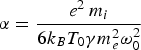 ${\rm \alpha}={{e^2\, m_i } \over {6k_B T_0 {\rm \gamma} m_e^2 {\rm \omega} _0^2 }}$ is nonlinearity parameter, N 0 is the density of plasma electrons in the absence of laser beam, k B is the Boltzmann's constant, T 0 is the equilibrium plasma temperature, and γ is the ratio of the specific heats. The pump wave equation in isotropic and homogeneous plasma can be described as;
 $$\nabla ^2 E - \nabla \left({\nabla .E} \right)+\displaystyle{{{\rm \varepsilon} \lpar r\comma \; z\rpar {\rm \omega} _0 ^2 } \over {c^2 }}\displaystyle{{\partial ^2 E} \over {\partial t^2 }}=0.$$
For transverse field ∇(∇.E) = 0. The solution in cylindrical coordinate can be described as
 $$E\lpar r\comma \; {\rm \theta}\comma \; z\rpar =E_0 \left({r\comma \; {\rm \theta}\comma \; z} \right)e^{ - i\left({k_0 z - {\rm \omega} _0 t} \right)} . $$
In the case of linear approximation, Eq. (2) will reduce to pure paraxial equation and taking the form (Mendonca et al., Reference Mendonca, Thide and Then2009),
 $$\left({\nabla _ \bot ^2+2ik_0 \displaystyle{\partial \over {\partial z}}} \right)E_0 \left({r\comma \; {\rm \theta}\comma \; z} \right)=0\comma \; $$
where 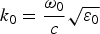 $k_0=\displaystyle{{{\rm \omega} _0 } \over c}\sqrt {{\rm \varepsilon} _0 } $ is wave vector and ω0 is frequency of the laser beam. The paraxial wave solution of Eq. (4) can be written as linear combination of the modes E 0 (r,θ, z) = E p,l (z) F p,l ( r,z )e ilθ, where F p,l ( r,z) is Laguerre-Gaussian function, integers p and l representing the radial and azimuthal numbers, respectively.
In case of nonlinear approximation, the dielectric constant ɛ ( r,z) is a function of intensity of the high power laser. The nonlinearity arises in plasma due to nonlinear dependence of the free carrier density on the electric field vector. For p ≥ 0 and l ≥ 1, laser beams propagation dynamics of Laguerre-Gaussian beam are complicated. For simplicity, we have taken HGBs, to understand the nature of the beams which have intensity null at center. The analysis of HGBs interaction with plasmas gives the general idea for higher order modes propagation inside the plasma. The initial field distribution of hollow Gaussian laser beam can be described by
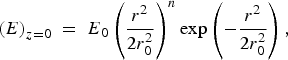 $$\left(E \right)_{z=0}\;=\;E_0 \left({\displaystyle{{r^2 } \over {2r_0 ^2 }}} \right)^n \exp \left({ - \displaystyle{{r^2 } \over {2r_0 ^2 }}} \right)\comma \; $$
where r 0 is the initial beam width, n is order of the HGBs, and E 0 is maximum amplitude of the laser beam around  $r=r_{\max }=r_0 \sqrt {2n}. $ Consider the solution of Eq. (2) is
 $$E_0 \left({r\comma \; z} \right)=\hat iA\left({r\comma \; z} \right)\exp \left({ - ik_0 z} \right)\comma \; $$
where A(r,z) is the complex amplitude of the wave and 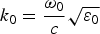 $k_0=\displaystyle{{{\rm \omega} _0 } \over c}\sqrt {{\rm \varepsilon} _0 } $. From Eqs. (2) and (6) we get,
 $$2ik_0 \displaystyle{{\partial A} \over {\partial z}}=\left({\displaystyle{{\partial ^2 A} \over {\partial r^2 }}+\displaystyle{1 \over r}\displaystyle{{\partial A} \over {\partial r}}} \right)+\displaystyle{{{\rm \omega} _0^2 } \over {c^2 }}\left({{\rm \varepsilon} - {\rm \varepsilon} _0 } \right)A. $$
The complex amplitude A(r,z) may be represented as
 $$A\left({r\comma \; z} \right)=A_0 \left({r\comma \; z} \right)\exp \left\{{ - ik_0 S_0 \left({r\comma \; z} \right)} \right\}. $$
Now transform the (r,z) coordinate in to ( η, z) coordinate as
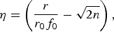 $${\rm \eta}=\left({\displaystyle{r \over {r_0 f_0 }} - \sqrt {2n} } \right)\comma \; $$
where r 0f 0 is width of pump beam and maximum irradiance is around 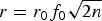 $r=r_0 f_0 \sqrt {2n} $; for the paraxial ray approximation
 ${\rm \eta} \ll \sqrt {2n}$ and A 0 is defined as
 $$A_0 ^2=\displaystyle{{E_0 ^2 } \over {2^{2n} f_0 ^2 }}\left({\sqrt {2n}+{\rm \eta} } \right)^{4n} \exp \left\{{ - \left({\sqrt {2n}+{\rm \eta} } \right)^2 } \right\}\comma \; $$
and eikonal of the beam is given as
 $$S_0 \left({{\rm \eta}\comma \; z} \right)=\displaystyle{{\left({\sqrt {2n}+{\rm \eta} } \right)^2 } \over 2}r_0 ^2 f_0 \displaystyle{{df_0 } \over {dz}}+{\rm \phi} \left(z \right). $$
The dimensionless beam width parameter f 0 can be obtained by using the initial boundary conditions f 0 | z=0 = 1 and df 0/dz| z=0 = 0, (Akhmanov et al., Reference Akhmanov, Sukhorukov and Khokhlov1968)
 $${\rm \varepsilon} _0 f_0 \displaystyle{{d^2 f_0 } \over {d{\rm \xi} ^2 }}=\displaystyle{4 \over {\,f_0 ^2 }} - {\rm \varepsilon} _2 {\rm \rho} _0 ^2 \comma \; $$
where  ${\rm \xi}=\displaystyle{c \over {r_0 ^2 {\rm \omega} _0 }}z$ is dimensionless parameter and
 ${\rm \rho} _0 ^2=\displaystyle{{r_0 ^2 {\rm \omega} _0 ^2 } \over {c^2 }}$. The plasma density varies through the plasma channel in presence of ponderomotive force, and the dielectric function ɛ(η, z) can be expressed as
 $$\eqalign{{\rm \varepsilon} \left({\rm \eta}\comma \; z \right)& = 1 - \displaystyle{{\rm \omega}_p^2 \over {\rm \omega}_0^2} \exp \left\{- \displaystyle{3 \over 4}{\rm \alpha} \displaystyle{m_e \over m_i} \displaystyle{{\rm E}_0^2 \over f_0^2} \left(\displaystyle{\left({\rm \eta} + \sqrt{2n} \right)^2 \over 2} \right)^{2n} \right. \cr & \quad\times \left.\exp \left\{- \left({\rm \eta} + \sqrt{2n} \right)^2 \right\}\right\}\comma \; } $$
ɛ0 (z) and ɛ2 (z) can be written as
 $$\hskip -56.5pt{\rm \varepsilon} _0 \left(z \right)=1 - \displaystyle{{{\rm \omega} _p ^2 } \over {{\rm \omega} _0 ^2 }}\left\{{\exp \left({ - \displaystyle{3 \over 4}{\rm \alpha} \displaystyle{{m_e } \over {m_i }}\displaystyle{{E_0 ^2 } \over {\,f_0 ^2 }}n^{2n} e^{ - 2n} } \right)} \right\}\comma \; $$
 $${{\rm \varepsilon} _2 \left(z \right)=2\left({\displaystyle{{{\rm \omega} _p ^2 } \over {{\rm \omega} _0 ^2 }}\displaystyle{3 \over 4}{\rm \alpha} \displaystyle{{m_e } \over {m_i }}\displaystyle{{E_0 ^2 } \over {\,f_0 ^2 }}n^{2n} e^{ - 2n} } \right)\exp \left({ - \displaystyle{3 \over 4}{\rm \alpha} \displaystyle{{m_e } \over {m_i }}\displaystyle{{E_0 ^2 } \over {\,f_0 ^2 }}n^{2n} e^{ - 2n} } \right).} $$
For the analysis of IAW, in presence of ponderomotive nonlinearity and filamented laser beam, the following equations are used. The equation of motion can be described as
 $$m_i\left[{\displaystyle{{\partial V_i } \over {\partial t}}+\left({V_i .\nabla } \right)V_i } \right]=eE+\displaystyle{e \over c}\left({V_i \times B} \right)- 2\Gamma _i m_i V_i - \displaystyle{{{\rm \gamma} _i \nabla {\rm P}} \over N}. $$
The Landau damping coefficient for IAW is given by Krall et al. (Reference Krall and Trivelpicec1973)
 $$\eqalign{2\Gamma _i &=\displaystyle{k \over {\left({1+k^2 {\rm \lambda} _d^2 } \right)}}\left({\displaystyle{{{\rm \pi} k_B {\rm T}_e } \over {8{m}_i}}} \right)^{1/2} \cr & \quad \times \left[{\left({\displaystyle{m \over { m}_i}} \right)^{1/2}+\left({\displaystyle{{{\rm T}_e } \over {{\rm T}_i }}} \right)^{3/2} \exp \left\{{ - \displaystyle{{{\rm T}_e } \over {{\rm T}_i \left({1+k^2 {\rm \lambda} _d^2 } \right)}}} \right\}} \right]\comma \; } $$
where 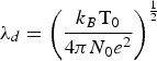 ${\rm \lambda} _d=\left({\displaystyle{{k_B {\rm T}_0 } \over {4{\rm \pi} N_0 e^2 }}} \right)^{{1 \over 2}}$ the Debye length and k is the wave vector of the acoustic wave. The continuity equation can be described as
 $$\displaystyle{{\partial N} \over {\partial t}}+\nabla \left({N.V_i } \right)=0. $$
Applying the perturbation approximation,
 $$N=N_0+n_{is}\comma \; V_{i}=v_{is} \, {\rm and}\, E=E_{H}+E_{si}\semicolon \; \, {\rm where}\, n_{is} \ll N_{0}.$$
From the Poisson's equation, one gets
 $$\nabla .E_{si}=- 4{\rm \pi} e\left({n_{es} - n_{is} } \right)$$
where n es is given by
 $$n_{es}=n_{is} \left[{1+k^2 {\rm \lambda} _d^2 \left({\displaystyle{{N_0 } \over {N_{0e} }}} \right)} \right]^{ - 1} .$$
From Eqs. (16), (18), and (19), one can obtain the general equation, which governs the ion density variation
 $$\eqalign{& \displaystyle{{\partial ^2 n_{is} } \over {\partial t^2 }}+2\mathop \Gamma \nolimits_i \displaystyle{{\partial n_{is} } \over {\partial t}} - c_s^2 \nabla ^2 n_{is} \cr & \quad + k^2 c_s^2 \left({ - 1+\displaystyle{1 \over {1+k^2 {\rm \lambda} _d^2 \left({\displaystyle{{N_0 } \over {N_{0e} }}} \right)}}} \right)n_{is} \simeq 0\comma \; } $$
where 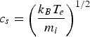 $c_s=\left({\displaystyle{{k_B T_e } \over m_i}} \right)^{1/2} $ is the speed of IAW for T e ≫ T i and assume that plasma is cold i.e., v thi2 ≪ c s2. Consider a plane wave solution of Eq. (21) is,
 $$n_{is}=n_i \left({r\comma \; z} \right)\exp \left\{{i\left({{\rm \omega} t - kz - S\left({r\comma \; z} \right)} \right)} \right\}\comma \; $$
where ω and k of the plasma wave satisfy the Bohm-Gross dispersion relation
 $${\rm \omega} ^2=\displaystyle{{k^2 c_s^2 } \over {1+k^2 {\rm \lambda} _d^2 \left({\displaystyle{{N_0 } \over {N_{0e} }}} \right)}}. $$
Using the value of n is from Eq. (22) in Eq. (21) and separating the real and imaginary part, one gets
 $$\eqalign{2\displaystyle{{\partial S} \over {\partial z}}+\left({\displaystyle{{\partial S} \over {\partial r}}} \right)^2 & =\displaystyle{1 \over {k^2 n_i }}\left\{{\displaystyle{1 \over r}\left({\displaystyle{{\partial n_i } \over {\partial r}}} \right)+\displaystyle{{\partial ^2 n_i } \over {\partial r^2 }}} \right\}\cr & \quad +\displaystyle{{{\rm \omega} ^2 } \over {k^2 c_s^2 }} \left\{{1 - \displaystyle{1 \over {1+k^2 {\rm \lambda} _d^2 \left({\displaystyle{{N_0 } \over {N_{0e} }}} \right)}}} \right\}\comma \; } $$
 $$\displaystyle{{\partial n_i ^2 } \over {\partial z}}+\displaystyle{{\partial S} \over {\partial r}}\left({\displaystyle{{\partial n_i ^2 } \over {\partial r}}} \right)+n_i ^2 \left\{{\displaystyle{1 \over r}\left({\displaystyle{{\partial S} \over {\partial r}}} \right)+\displaystyle{{\partial ^2 S} \over {\partial r^2 }}} \right\}+\displaystyle{{2\Gamma i} \over {c_s^2 }}\displaystyle{{{\rm \omega} n_i ^2 } \over k}=0. $$
Eqs. (24) and (25) can be solved in paraxial ray approximation (for initial HGB distribution), after transforming (r, z) coordinate in to (η, z) coordinate using Eq. (9), one can find,
 $$\eqalign{n_i^2 &=\displaystyle{{n_0^2 } \over {\,f^2 2^{2n} }}\left({{\rm \eta}+\sqrt {2n} } \right)^{4n} \left({\displaystyle{{r_0 f_0 } \over {af_e }}} \right)^{4n} \exp \left({ - \left({{\rm \eta}+\sqrt {2n} } \right)^2 - 2k_i z} \right).} $$
And the eikonal of the IAW is
 $$S=\left({{\rm \eta}+\sqrt {2n} } \right)^2 \displaystyle{{r_0^2 f_0^2 } \over {2f}}\displaystyle{{\partial f} \over {\partial z}}+{\rm \phi} \left(z \right)\comma \; $$
where  $k_i=\displaystyle{{\Gamma _i {\rm \omega} } \over {kc_s^2 }}$ is damping factor, f and a are the dimensionless beam width parameter and radius of IAW, respectively. The dimensionless beam width parameter f can be obtained by using the boundary conditions f|z=0 = 1 and df/dz|z=0 = 0,
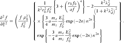 $$\eqalign{\displaystyle{{\partial ^2 f} \over {\partial {\rm \xi} ^2 }} & =\left({\displaystyle{{\mathop {\,f\,{\rm \rho} }\nolimits_0^2 } \over {\mathop f\nolimits_0^2 }}} \right)\left\{\matrix{\displaystyle{1 \over {k^2 r_0^2 f_0^2 }}\left\{{3+\left({\displaystyle{{r_0 f_0 } \over {af}}} \right)^4 } \right\}- 2\displaystyle{{k^2 {\rm \lambda} _d^2 } \over {\left({1+k^2 {\rm \lambda} _d^2 } \right)^2 }} \hfill \cr \times \left\{{\displaystyle{3 \over 4}{\rm \alpha} \displaystyle{{m_e } \over {m_i }}\displaystyle{{E_0^2 } \over {\,f_0^2 }}\exp \left({ - 2n} \right)n^{2n} } \right\}\hfill \cr \exp \left\{{ - \displaystyle{3 \over 4}{\rm \alpha} \displaystyle{{m_e } \over {m_i }}\displaystyle{{E_0^2 } \over {\,f_0^2 }}\exp \left({ - 2n} \right)n^{2n} } \right\}\hfill} \right\}.} $$
3. STIMULATED BRILLOUIN SCATTERING
The high frequency electric field ET can be written as the sum of the electric fields of scattered wave ES and the electric field of pump laser beam Ei.
 $${\rm E}_{\rm H}={\rm E}_i e^{i{\rm \omega} _0 t}+{\rm E}_S e^{i{\rm \omega} _s t} \comma \; $$
where ω0 and ωS are the incident laser beam and scattered wave frequencies, respectively. The wave equation for the scattered field can be written as
 $$\nabla ^2 E_s - \displaystyle{{{\rm \omega} _s ^2 } \over {c^2 }}\left({1 - \displaystyle{{{\rm \omega} _p ^2 } \over {{\rm \omega} _s ^2 }}\displaystyle{{N_{0e} } \over {N_0 }}} \right)E_s=\displaystyle{{{\rm \omega} _p ^2 } \over {2c^2 }}\displaystyle{{{\rm \omega} _s } \over {{\rm \omega} _0 }}\displaystyle{{n_{es} ^\ast } \over {N_0 }}E_i . $$
The solution of Eq. (30) can be written as
 $$E_s=E_{s0} \left({r\comma \; z} \right)e^{ik_{s0} z}+E_{s1} \left({r\comma \; z} \right)e^{ - ik_{s1} z} \comma \; $$
where 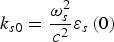 $k_{s0}=\displaystyle{{{\rm \omega} _s ^2 } \over {c^2 }}{\rm \varepsilon} _s \left(0 \right)$, k S1, and ωS are satisfies they phase matching conditions.
 $$k_{S1}=k_0 - k\comma \; {\rm \omega} _S={\rm \omega} _0 - {\rm \omega} . $$
From Eqs. (30) and (31), one gets
 $$\left({\displaystyle{1 \over r}\displaystyle{{\partial {\rm E}_{S0} } \over {\partial r}}+\displaystyle{{\partial ^2 {\rm E}_{S0} } \over {\partial r^2 }}} \right)+2ik_{S0} \displaystyle{{\partial {\rm E}_{S0} } \over {\partial z}} - k_{S0}^2 {\rm E}_{S0}+\displaystyle{{{\rm \omega} _S^2 } \over {c^2 }} \in _S \left({r\comma \; z} \right){\rm E}_{S0}=0\comma \; $$
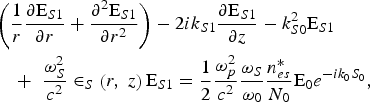 $$\eqalign{& \left({\displaystyle{1 \over r}\displaystyle{{\partial {\rm E}_{S1} } \over {\partial r}}+\displaystyle{{\partial ^2 {\rm E}_{S1} } \over {\partial r^2 }}} \right)- 2ik_{S1} \displaystyle{{\partial {\rm E}_{S1} } \over {\partial z}} - k_{S0}^2 {\rm E}_{S1} \cr & \quad +\,\,\displaystyle{{{\rm \omega} _S^2 } \over {c^2 }} \in _S \left({r\comma \; z} \right){\rm E}_{S1}=\displaystyle{1 \over 2}\displaystyle{{{\rm \omega} _p^2 } \over {c^2 }}\displaystyle{{{\rm \omega} _S } \over {{\rm \omega} _0 }}\displaystyle{{n_{es} ^ \ast } \over {N_0 }}{\rm E}_0 e^{ - ik_0 S_0 } \comma \; } $$
where 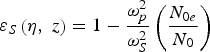 ${\rm \varepsilon} _S \left({{\rm \eta}\comma \; z} \right)=1 - \displaystyle{{{\rm \omega} _p^2 } \over {{\rm \omega} _S^2 }}\left({\displaystyle{{N_{0e} } \over {N_0 }}} \right)$, to simplify the Eq. (33), one substitute ES0 = ES00 (r,z)e ik S0S c in Eq. (33) and separating the real and imaginary part as
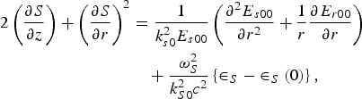 $$\eqalign{2\left({\displaystyle{{\partial S} \over {\partial z}}} \right)+\left({\displaystyle{{\partial S} \over {\partial r}}} \right)^2 & =\displaystyle{1 \over {k_{s0} ^2 E_{s00} }}\left({\displaystyle{{\partial ^2 E_{s00} } \over {\partial r^2 }}+\displaystyle{1 \over r}\displaystyle{{\partial E_{r00} } \over {\partial r}}} \right)\cr & \quad +\displaystyle{{{\rm \omega} _S ^2 } \over {k_{S0}^2 c^2 }}\left\{{ \in _S - \in _S \left(0 \right)} \right\}\comma \; } $$
 $$\displaystyle{{\partial E_{s00} ^2 } \over {\partial z}}+E_{s00} ^2 \left({\displaystyle{{\partial ^2 S_0 } \over {\partial r^2 }}+\displaystyle{1 \over r}\displaystyle{{\partial S_0 } \over {\partial r}}} \right)+\left({\displaystyle{{\partial E_{s00} ^2 } \over {\partial r}}} \right)\left({\displaystyle{{\partial S_0 } \over {\partial r}}} \right)=0. $$
Eqs. (35) and (36) can be solved in paraxial ray approximation (for initial HGB distribution), after transforming (r, z) coordinate in to (η, z) coordinate using Eq. (9), one can find,
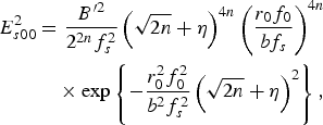 $$\eqalign{E_{s00} ^2 & =\displaystyle{{B^{\prime 2} } \over {2^{2n} f_s ^2 }}\left({\sqrt {2n}+{\rm \eta} } \right)^{4n} \left({\displaystyle{{r_0 f_0 } \over {bf_s }}} \right)^{4n} \cr & \quad \times \exp \left\{{ - \displaystyle{{r_0^2 f_0^2 } \over {b^2 f_s^2 }}\left({\sqrt {2n}+{\rm \eta} } \right)^2 } \right\}\comma \; } $$
 $$S_c=\displaystyle{{\left({\sqrt {2n}+{\rm \eta} } \right)^2 } \over 2}\displaystyle{{r_0^2 f_0^2 } \over {\,f_s }}\displaystyle{{\partial f_s } \over {\partial z}}+{\rm \phi} _s \left(z \right). $$
Using the Eqs. (37) and (38) in Eq. (35) and equating the coefficient of η2, one can get
 $$\displaystyle{{d^2 f_s } \over {d{\rm \xi} ^2 }}=\displaystyle{{\mathop {\rm \rho} \nolimits_0^2 f_s } \over {\,f_0^2 }}\left\{{\displaystyle{1 \over {k_{S0}^2 r_0^2 f_0^2 }}\left\{{3+\left({\displaystyle{{r_0 f_0 } \over {bf_s }}} \right)^4 } \right\}- \displaystyle{{{\rm \omega} _s^2 } \over {k_{s0}^2 c^2 }} \in _{S2} } \right\}. $$
Here, we used the boundary condition 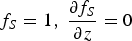 $f_S=1\comma \; \displaystyle{{\partial f_S } \over {\partial z}}=0$. In presence of ponderomotive nonlinearity, the ɛS (η, z) may be expressed as
 $${\rm \varepsilon} _S \left({{\rm \eta}\comma \; z} \right)={\rm \varepsilon} _S \left(0 \right)- {\rm \eta} ^2 {\rm \varepsilon} _{S2} \comma \; $$
where
 $${\rm \varepsilon} _S \left(0 \right)=1 - \displaystyle{{{\rm \omega} _p^2 } \over {{\rm \omega} _S^2 }}\left\{{\exp \left({ - \displaystyle{3 \over 4}{\rm \alpha} \displaystyle{{m_e } \over {m_i }}\displaystyle{{E_0 ^2 } \over {\,f_0 ^2 }}n^{2n} e^{ - 2n} } \right)} \right\}\comma \; $$
 $${\rm \varepsilon} _{S2}=1 - \displaystyle{{{\rm \omega} _p^2 } \over {{\rm \omega} _S^2 }}\left\{{\exp \left({ - \displaystyle{3 \over 4}{\rm \alpha} \displaystyle{{m_e } \over {m_i }}\displaystyle{{E_0 ^2 } \over {\,f_0 ^2 }}n^{2n} e^{ - 2n} } \right)} \right\}. $$
The value of B ′ can be obtained on applying appropriate boundary condition
 $${\rm E}_S={\rm E}_{S0} \left({r\comma \; z} \right)e^{ik_{S0} z}+{\rm E}_{S1} \left({r\comma \; z} \right)e^{ - ik_{S1} z}=0 _{{\rm at}\ z=z_c} \comma \;$$
where, z c = L − z and L is the interaction length. Here, z c is chosen sufficiently large so that n i is nearly zero. Therefore, at z = z c, one gets
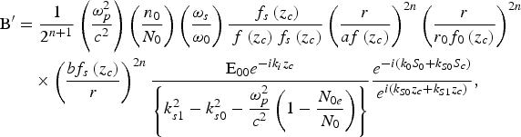 $$\eqalign{ {\rm B}^{\prime}&=\displaystyle{1 \over {2^{n+1} }}\left({\displaystyle{{{\rm \omega} _p^2 } \over {c^2 }}} \right)\left({\displaystyle{{n_0 } \over {N_0 }}} \right)\left({\displaystyle{{{\rm \omega} _s } \over {{\rm \omega} _0 }}} \right)\displaystyle{{\,f_s \left({z_c } \right)} \over {\,f\left({z_c } \right)f_s \left({z_c } \right)}}\left({\displaystyle{r \over {af\left({z_c } \right)}}} \right)^{2n}\left({\displaystyle{r \over {r_0 f_0 \left({z_c } \right)}}} \right)^{2n} \cr & \quad \times \left({\displaystyle{{bf_s \left({z_c } \right)} \over r}} \right)^{2n} \displaystyle{{{\rm E}_{00} e^{ - ik_i z_c } } \over {\left\{{k_{s1}^2 - k_{s0}^2 - \displaystyle{{{\rm \omega} _p^2 } \over {c^2 }}\left({1 - \displaystyle{{N_{0e} } \over {N_0 }}} \right)} \right\}}}\displaystyle{{e^{ - i\left({k_0 S_0+k_{S0} S_c } \right)} } \over {e^{i\left({k_{S0} z_c+k_{S1} z_c } \right)} }},} $$
with the condition
 $${1 \over {a^{2} f^{2} (z_c )}} \ +\ {1 \over {r_{0} ^{2} f_0^{2} (z_c )}}\ =\ {1 \over {b^{2} f_{s}^{2} (z_{c} )}}. $$
Back reflectivity of SBS process can be defined as the ratio of back scattered power to the incident power and is given by
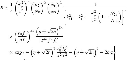 $$\eqalign{R & \simeq \displaystyle{1 \over 4}\left({\displaystyle{{{\rm \omega} _p ^2 } \over {c^2 }}} \right)^2 \left({\displaystyle{{n_0 } \over {N_0 }}} \right)^2 \left({\displaystyle{{{\rm \omega} _s } \over {{\rm \omega} _0 }}} \right)^2 \displaystyle{1 \over {\left\{{k_{s1} ^2 - k_{s0} ^2 - \displaystyle{{{\rm \omega} _p ^2 } \over {c^2 }}\left({1 - \displaystyle{{N_{0e} } \over {N_0 }}} \right)} \right\}^2 }} \cr & \quad \times \left({\displaystyle{{r_0 f_0 } \over {af}}} \right)^{4n} \displaystyle{{\left({{\rm \eta}+\sqrt {2n} } \right)^{8n} } \over {2^{4n} f^2 f_0^2 }}\cr & \quad \times \,\exp \left\{{ - \left({{\rm \eta}+\sqrt {2n} } \right)^2 \displaystyle{{r_0^2 f_0^2 } \over {a^2 f^2 }} - \left({{\rm \eta}+\sqrt {2n} } \right)^2 - 2k_i z} \right\}} $$
4. RESULT AND DISCUSSION
The density of the plasma varies due to the ponderomotive force in the collisionless plasma and the refractive index increases at the position of the maximum irradiance. Eqs. (10) and (12) show the intensity profile of HGBs in plasma along the radial direction in presence of ponderomotive nonlinearity. The intensity profile of the pump beam varies with the dimensionless beam width parameter f 0 in the paraxial regime. In Eq. (12), on the right-hand side, first term is responsible for diffraction, while the second term (nonlinear term) is responsible for the converging behavior of the beam propagation in plasma. For numerical calculation, we have used the following typical laser beam parameters: the vacuum wavelength of the laser beam (λ = 1064 nm), laser power flux (1016 W/cm2), the initial radius of the laser beam, r 0 = 10 μm, the initial radius of the IAW, a = 10 μm, plasma density, n/n cr = 0.2 and v th = 0.1c. Eq. (12) has been solved for a HGB and the numerical results are presented in Figures 1, 2, and 3. Figures 1a, 2a, and 3a show the intensity of HGBs for order 1, 2, and 3, respectively at ξ = 0. Figures 1b, 2b, and 3b show the intensity variation of HGBs for order 1, 2, and 3 at first focal point (beam focused position) with normalized distance ξ, respectively. The intensity of laser beams is maximum at η = 0; and at first focal point the intensity of HGBs decrease with increase the order of the HGBs.
(Color online) Normalized intensity distribution for order 1. (a) HGB and IAW at ξ = 0, (b) HGB at first focal point, (c) IAW at first focal point, (d) Back SBS at first focal point.

(Color online) Normalized intensity distribution for order 2. (a) HGB and IAW at ξ = 0, (b) HGB at first focal point, (c) IAW at first focal point, (d) Back SBS at first focal point.
(Color online) Normalized intensity distribution for order 3. (a) HGB and IAW at ξ = 0, (b) HGB at first focal point, (c) IAW at first focal point, (d) Back SBS at first focal point.
The motion of the charge carrier will be modified due to ponderomotive nonlinearity and will give rise to change in the nonlinear current density. The density profile of IAW can be modified and governed by the Eq. (26). We have solved Eq. (28) numerically to obtain the amplitude of the density perturbation at finite z. In the collision-less plasma, the right side of Eq. (28) describes the variation in the dimensionless beam width parameter f of IAW on account of the competition between diffraction and non-linear terms with the distance of propagation. The results are displayed in Figures 1a, 2a, and 3a show that the IAW gets excited due to nonlinear coupling with high power laser beam in presence of the ponderomotive non-linearity of order 1, 2, and 3, respectively. The IAW is also having the maximum intensity (for different order of HGBs) at η = 0 in the paraxial regime. Figures 1c, 2c, and 3c show the variation in intensity for order 1, 2, and 3 of IAW at first focal point respectively, with normalized distance ξ.
Eq. (39) describes the variation of beam width parameter of the scattered beam and Eq. (45) gives the back reflectivity of SBS process against the distance of propagation. The right-hand side of Eq. (39) represents the variation in the dimensionless beam width parameter f s which arises due to the competition between non-linear and diffraction term with the distance of propagation in the collisionless plasma. The results are displayed in Figures 1d, 2d, and 3d show the normalized intensity (normalized by pump intensity) of the back reflected laser beam at the focal point for order 1, 2, and 3, respectively. We have solved Eq. (45) numerically to obtain the back reflectivity with normalized distance ξ for different order of HGBs around the maximum irradiance η = 0. Figure 4 shows that the back reflectivity decreases with increasing order of the HGBs because the focusing of HGBs decreases with increasing order of the HGBs beam. The fluctuations in the reflectivity are on the account of minima in the dimensionless beam width parameters of laser beam and ion acoustic beam.
(Color online) Variation of back reflectivity against normalized distance of propagation ξ.
5. CONCLUSION
We studied the excitation and self-focusing of IAW in the presence of HGBs. The focusing of the HGBs, excitation of IAW and back reflectivity for SBS process has been investigated for higher order modes of HGBs. The analysis clearly shows that the back reflectivity decreases at the focused positions for higher order modes of HGBs because the focusing of HGBs and IAW decrease for higher order modes. The results are useful for understanding the physics of laser induced fusion in which the laser beam is superposition of higher order modes.
ACKNOWLEDGMENT
This work was partially supported by University Grant Commission (UGC), India and Department of Science and Technology (DST), India.



