2. CLUSTERING

Clustering in statistics and machine learning is one of the unsupervised learning methods that deals with finding a structure in a collection of unlabelled data (Murphy, Reference Murphy2012) and dividing it into categories with similar members, called clusters. The lack of a precise definition of the cluster is one of the reasons why there are several clustering algorithms. Practically, there is not a completely objective and correct clustering algorithm for each subject, as clustering is in the eye of the beholder (Estivill-Castro, Reference Estivill-Castro2002). In other words, the best clustering algorithm for a particular problem should often be empirically selected unless there is a mathematical or logical reason to prefer one algorithm to another. Meanwhile, according to the definition of the intended problem (star catalogue uniformity), the centroid clustering algorithms are the most suitable methods for the problem investigated here.

In centroid clustering, the clusters are represented by a central vector which may not necessarily be part of the dataset. In this method, the goal is to decompose n observations to the completely separated k clusters in order to increase the similarity of each cluster and simultaneously decrease the similarity between different clusters. This similarity was measured by using various criteria such as Euclidean, Manhattan, Maximum and so on, and each observation is attributed to the cluster with the closest criterion relative to the cluster centre.

One of the most applied and oldest algorithms used in centroid clustering is k-means (Hartigan and Wong, Reference Hartigan and Wong1979), which is a greedy algorithm and uses metaheuristic methods to solve the problem. The differentiation criterion in the classical k-means algorithm is the squared Euclidean distance by using the following objective function (Jain, Reference Jain2010):

(1)$$J_{KM}=\sum\limits_{j=1}^k \sum\limits_{i=1}^n \left\Vert x_{i}^{(j)}-c_{j} \right\Vert _{2}^{2}$$

where ‖.‖₂ is the Euclidean norm and the criterion of the distance between the j-th cluster centre (c _j) and the element i of this cluster $(x_{i}^{(j)})$.

The most important assumption and somewhat an objection in the k-means algorithm is that the initial number and location of the clusters should be specified from the beginning and the final answer is sensitive to the selection of the initial clusters (Bagirov, Reference Bagirov2008). On the other hand, the main advantage of the k-means method is that this algorithm produces tighter clusters compared to many other clustering methods such as hierarchical clustering (Sonagara and Badheka, Reference Sonagara and Badheka2014), especially when the data are normalised. In this regard, the Spherical K-Means (SKM) algorithm presented in Dhillon and Modha (Reference Dhillon and Modha2001) is an exploratory, simple and fixed-point method for minimising the cost function of 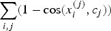$\sum_{i,j} (1-\cos(x_{i}^{(j)},c_{j}))$ (Buchta et al., Reference Buchta, Kober, Feinerer and Hornik2012). Actually, the distance criterion used in the k-means method is replaced with cosine similarity of the corresponding angles in the spherical k-means algorithm.

(2)$$J_{SKM}=\sum_{j=1}^k \sum_{i=1}^n \lpar 1-\langle x_i^{(j)},c_j\rangle \rpar $$

Therefore, it appears that the SKM algorithm can be used to generate a uniform star catalogue on the celestial sphere because the star catalogue data have the same characteristics, but, as mentioned earlier, different criteria have been suggested and used by researchers for clustering and selecting each of these criteria, and these affect the shape of clusters and the results. Hence, a novel criterion called the geodesic distance is introduced for clustering by the k-means method on the sphere.

In differential geometry, a curve α in a geometric surface M is called the geodesic of M provided its acceleration is zero (O'Neill, Reference O'Neill1966). Therefore, the geodesics are the most direct curves and without any twisting. In fact, the geodesic is the shortest curve adjoining two given points on a surface (Hirvonen, Reference Hirvonen1961).

3. GEODESIC K-MEANS CLUSTERING

It has been shown that cosine similarity is a superior measure to Euclidean distance for high-dimensional data such as text documents and market baskets (Zhong, Reference Zhong2005), which means that the direction of the observation vector is more important than its size. Accordingly, in SKM the goal is to maximise the cosine similarity of a cluster. However, the aim of the proposed algorithm is to use the shortest distance criterion on the sphere surface. In Geodesic K-Means (GKM) clustering, the geodesic is used as the shortest path between two points on the surface and the goal is to minimise the cost function:

(3)$$J_{GKM}=\sum_{j=1}^k \sum_{i=1}^n d\lpar x_{i}^{(j)},c_{j}\rpar $$

where d(a, b) refers to the geodesic distance and can be extended to an ellipsoid or any other arbitrary surface.

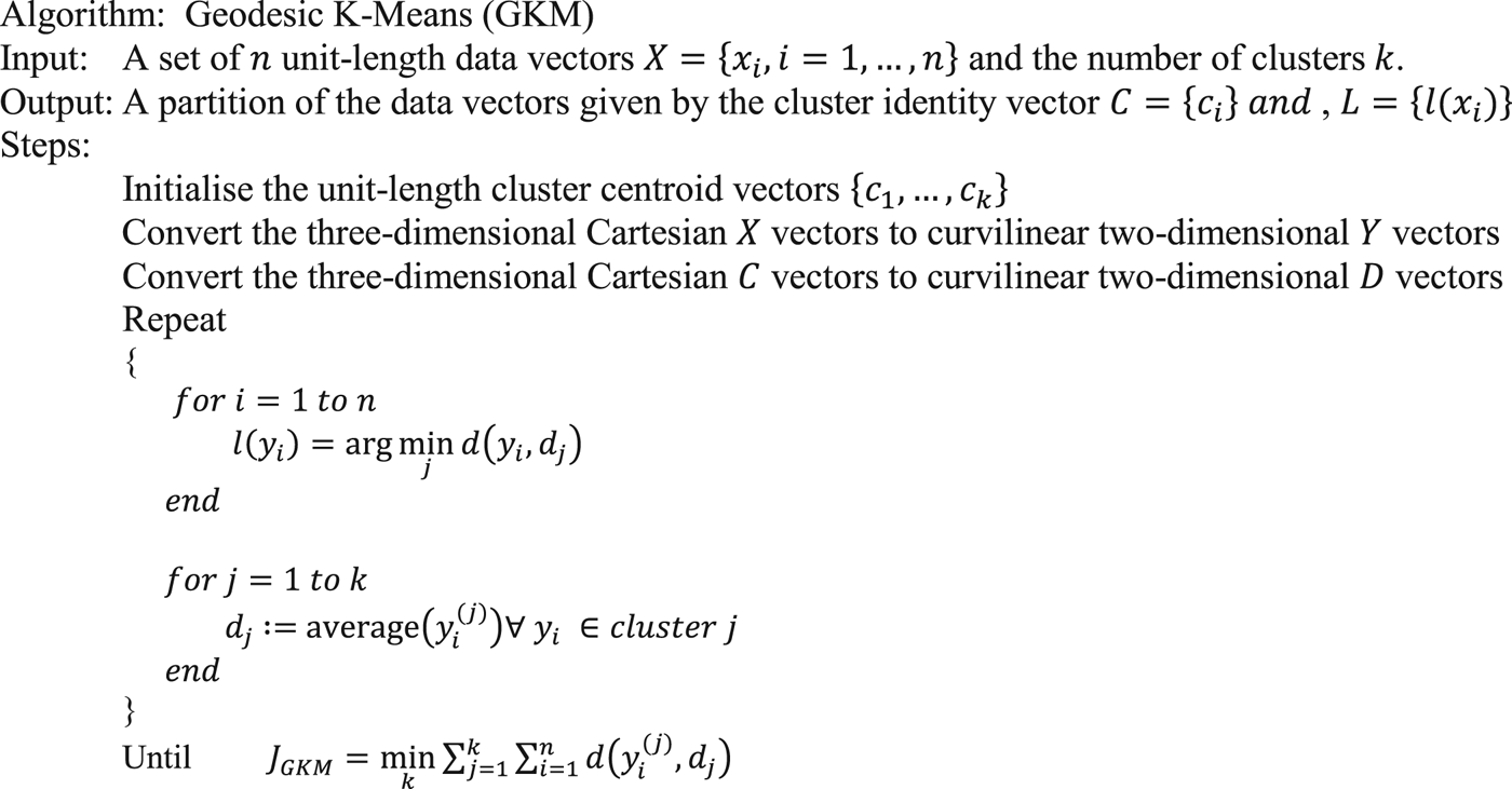
Thus, the proposed algorithm is as follows: the three-dimensional coordinates of the observations are first converted to the two-dimensional curvilinear coordinates by using Equation (4):

(4)$$\alpha=tan^{-1}\displaystyle{x_{i2} \over x_{i1}},\quad \delta = tan^{-1}\displaystyle{x_{i3} \over \sqrt{x_{i1}^{2}+x_{i2}^{2}}}$$

Then, k points (from observations, randomly, or using the uniform distribution methods such as triangulation) are considered as the first centres of clusters. Then, for all observations X = {x _i, i = 1, …, n}, the geodesic distance to the centre of the clusters is calculated and each observation is assigned to a cluster based on the shortest distance. Finally, for each cluster, the average of its elements is selected as the new cluster centre and the algorithm continues to satisfy the convergence condition. Figure 1 presents the pseudo code.

Figure 1.

Geodesic k-means clustering algorithm.

There is an obvious relationship between cosine similarity and Euclidean distance (Hopcroft and Kannan, Reference Hopcroft and Kannan2014). The proposed method extends the use of the k-means clustering algorithm to other surfaces such as ellipsoid surfaces. On the other hand, the problems of this algorithm, many of which are also common among other k-means derivatives, are as follows:

1. 1. This method sometimes ends in a local optimality.

2. 2. The GKM method is only used when the average of the data can be defined and accordingly it is not suitable for qualitative data.

3. 3. This method is sensitive to determining the number and the location of the initial centres of clusters and consequently the final result depends on this initialisation.

4. 4. The GKM method is sensitive to noise and outlier data, and no matter how small the outlier is, it still has a great impact on the average clusters.

4. TRIANGULATION

Since the proposed clustering method is sensitive to the initial number and location of the cluster centres, for catalogue uniformity, it is required to generate the equidistribution initial points on a unit sphere and guarantee the possibility of repeatability of the results. An effective method is using patches to cover the surface of a unit sphere. Obviously, using simplex is the best method to optimally cover the surface of the unit sphere. Since the pyramid is the simplest possible geometric shape in ℝ³, the use of a pyramid or, in fact, triangles forming the pyramid is a suitable method for the optimal covering of the unit sphere, the so-called triangulation.

In Euclidean geometry, the triangulation of the set of points H in ℝⁿ is a simplicial complex which covers the surface of the points H, and its vertices belong to H (De Loera et al., Reference De Loera, Rambau and Santos2010). In addition, some references bind that all points in the H should be the vertices of the triangles without overlap (De Berg et al., Reference De Berg, Van Kreveld, Overmars and Schwarzkopf2000). Finally, the most important issue in triangulation is the lack of dependence of the algorithm on the starting point or justification of the initial points and the results should be replicable and predictable. Hence, the Delaunay triangulation method (Delaunay, Reference Delaunay1934) was used to produce equidistributed points in this research. In this method, the triangulation is performed to satisfy the condition of the empty peripheral circle.

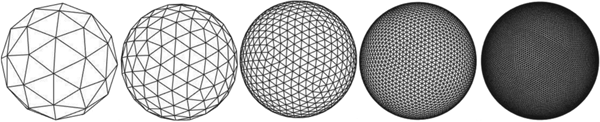
Currently, various methods are presented for solving Delaunay triangulation problems, and the incremental method is more popular, is simpler and has higher precision among the available algorithms (Kohout et al., Reference Kohout, Kolingerová and Žára2005). One of the most widely used algorithms in this field is the STRIPACK (Spherical TRIangulation PACKage) algorithm, which is also used in the present study. STRIPACK is an incremental algorithm for generating Delaunay triangles for a set of points on a unit sphere and it has been shown that using an off-line algorithm and work space of size 3n, the triangulation can be constructed with time complexity O(nlog n) (Renka, Reference Renka1997). Figure 2 illustrates some examples of the spheres created with this algorithm and different initial parameters.

Figure 2.

The nodes generated by the STRIPACK algorithm and different resolutions.

5. SCATTERED DATA DENSITY

The distribution of stars in the celestial sphere is not even or random: the distribution near the celestial pole is sparse while that near the equator is relatively dense (Zhang, Reference Zhang2017). Applying the same procedure of uniformity with a constant resolution to all areas of the sky is unreasonable, and it is possible to apply different resolutions of triangulation (Figure 2) for different areas of the sky. Therefore, in the proposed method, an attempt was made to make the uniformity process softer and more targeted by using the determination of the scattered data density.

In basic sciences, the density of scattered data is the number of data in the sampling unit (volume, area, etc.). Since the density depends on the areas, the calculation process should be performed in such a way that the measurement areas are minimised. On the other hand, the generalisation of the subject requires that the measurement areas are not limited to circles or any other geometric shapes and have arbitrary shapes and sizes, so theVoronoi diagram method is used for this purpose.

According to its definition, the Voronoi diagram VD(P) of a set P = {p ₁, …, p _n} of points in ℝ² is the subdivision of the plane induced by the Voronoi cells V _p(i), for i=1, …, n (Gärtner and Hoffmann, Reference Gärtner and Hoffmann2013), so that V _p(i) is composed of a set R _k = {xεℝ²|d(x, P _k) ≤ d(x, P _j) for all j≠k} of points and is a distance function in ℝ² (mostly Euclidean norm). In fact, a Voronoi diagram is a partitioning of a plane with points into convex polygons such that each polygon contains exactly one generating point and every point in a given polygon is closer to its generating point than to any other.

Thus, the main idea in determining scattered data density is that the area occupied by each element is calculated by using the area of the corresponding Voronoi cell (Plaue et al., Reference Plaue, Bärwolff and Schwandt2014). In this method, the Voronoi diagram is first calculated for scattered data $\vec{x}=\{\vec{x}_{i}\in \open{R}^{2}\}$, and then the cell area $\vert A_{i}\vert = \int_{A} d\vec{x}$ is calculated for all closed polygons derived from the Voronoi diagram. Hence, the distribution of the point density is defined for each star as follows (Steffen and Seyfried, Reference Steffen and Seyfried2010):

(5)$$p_{i}(\vec{x}) = \left\{\matrix{\displaystyle{1 \over A_{i}}: \hfill & if \vec{x}\in A_{i} \hfill \cr 0: \hfill & otherwise \hfill} \right. \quad and \quad p(\vec{x})=\sum_i p_{i}(\vec{x})$$

In general, the non-negative function $p_{i}(\vec{x})$ is not a continuous function, and without applying certain restrictions on the cell size, 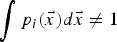$\int {p_{i}(\vec{x})} d\vec{x}\ne 1$. Therefore, in practice, a convolution with a two-dimensional moving average filter is used for smoothing and the density in the area is defined as (Steffen and Seyfried, Reference Steffen and Seyfried2010):

(6)$$D=\displaystyle{\int_{A}p(\vec{x})d\vec{x} \over \vert A\vert}$$

6. CATALOGUE UNIFORMITY

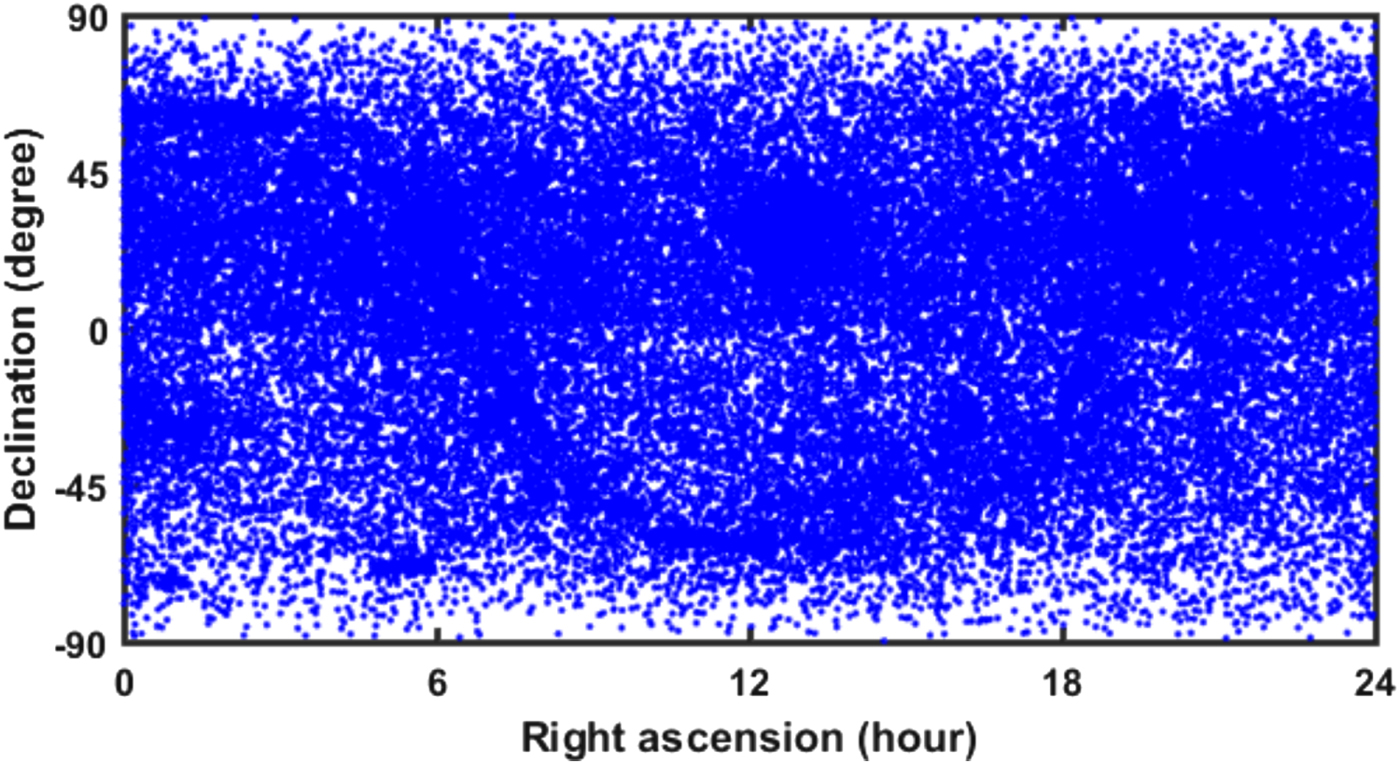
In the first step, it is necessary to select an appropriate star catalogue and extract the required data. Therefore, after reviewing the catalogues used in some operational sensors and in Roshanian et al. (Reference Roshanian, Hasani, Yazdani and Ebrahimi2015b), the Hipparcos catalogue was used as a reference catalogue (Figure 3).

Figure 3.

Hipparcos Reference catalogue.

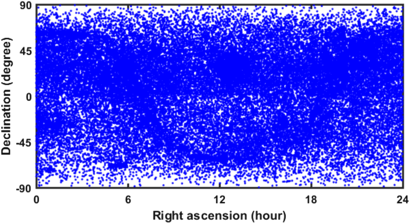
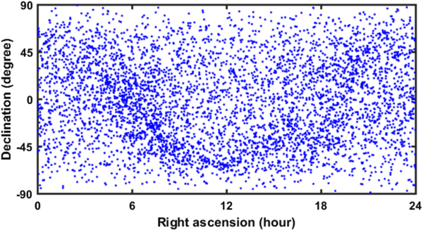
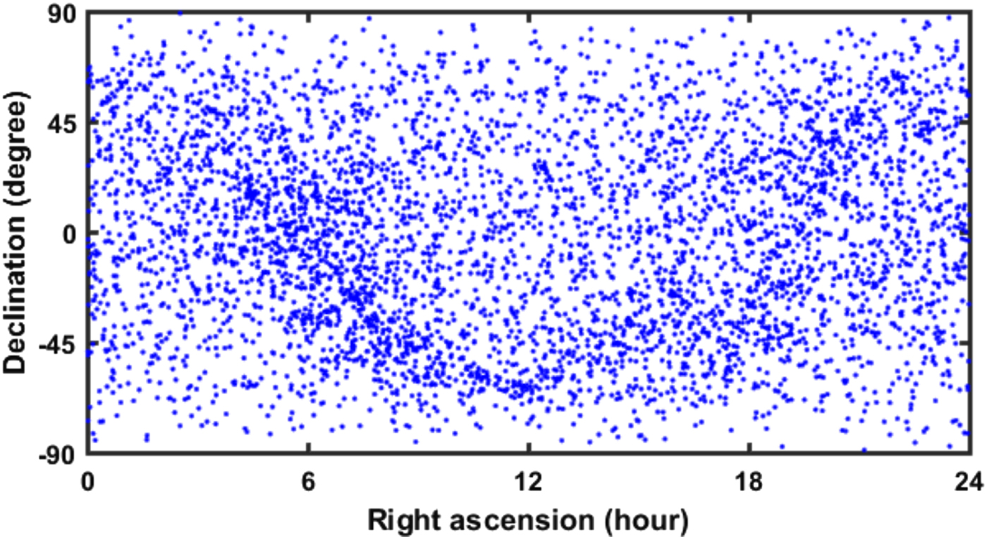
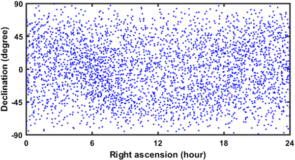
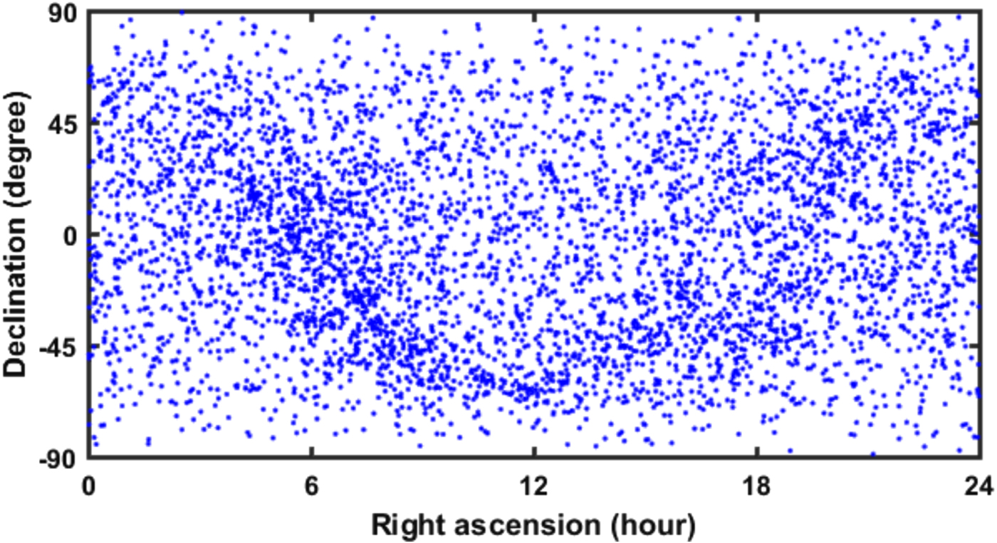
In the next step, the reference star catalogue was first limited based on the minimum magnitude to reduce the size of the database by the sensitivity of the detector. Although this minimum magnitude is related to the detector sensitivity, its value is usually within the brightness range of stars visible with the naked eyes, which is about six (Martín-Fleitas et al., Reference Martín-Fleitas, Mora, Sahlmann, Kohley, Massart, L'hermitte, Roy and Paulet2014). Limiting the reference catalogue to magnitude six resulted in decreasing the number of stars to 5,176 (Figure 4).

Figure 4.

Limited catalogues for stars brighter than magnitude 6.

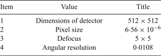
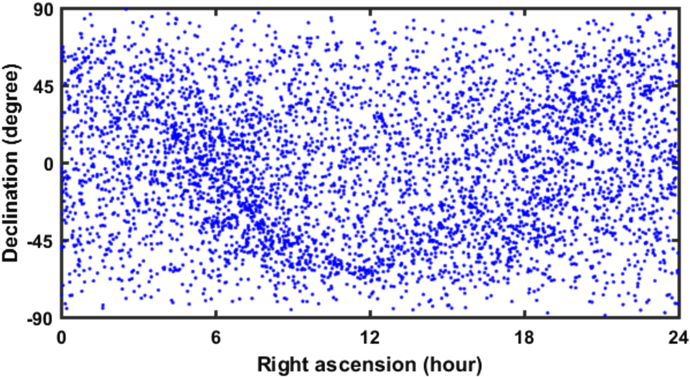
In the third step, due to the problems caused by “double” stars in the identification phase, an attempt was made to exclude these stars from the database. In astronomy “double” stars is a different concept from that of binary stars. Astronomically, binary stars are two stars that are close to and revolve around each other (Zhang, Reference Zhang2017), but in the present study, “double” stars refer to two stars which may be relatively distant in reality although their images on the detector are not distinguishable by a centroiding algorithm. The size of the star spot (due to the star magnitude and the defocus of the optical system) is of great importance, so the quantity of the angular resolution of the optical system is used to determine the double stars.

(7)$$\theta_{angular\ resolution}=2\times \Delta \times tan\left(\displaystyle{ps \over 2\times f} \right)$$

where f represents the focal length, ps indicates the pixel size, and Δ shows the distribution of the star spot due to the defocus. Based on the parameters of Table 1, if the spatial angle between the two stars is smaller than the angular resolution of the optical system, both stars would be removed from the limited catalogue (Figure 4). Thus, the number of stars in the catalogue limited to magnitude six was reduced to 4,729 stars after removing double stars (Figure 5).

Figure 5.

Removing double stars.

Table 1.

Specifications of the optical system used in the research.

In the final step, since the density of stars is not the same in the entire celestial sphere (Figures 3, 4 and 5) and regarding the minimum stars required for the identification algorithm, we tried to remove additional dimmer stars from the database. This process is called achieving catalogue uniformity, which means reducing the size of the database and increasing the reliability of the identification algorithm.

It is clear that no process can be practically performed for uniformity in areas of the sky with low star densities. However, in denser areas, it is possible to eliminate some dimmer stars to provide the appropriate density. To this end, geodesic k-means clustering is proposed.

At first in order to generate the uniform star catalogue using the GKM method, the surface of the celestial sphere was covered by using the Delaunay triangulation method with 9,002 equidistribution points (equal to initial parameter 30). Then, these initial points with a catalogue limited to magnitude six and the removal of double stars (Figure 5) were input into the GKM uniformity algorithm. In this step, due to the importance of star magnitude in the process of catalogue uniformity, the magnitude of each star was applied to the geodesic clustering algorithm as a weight parameter and the Geodesic Weighted K-Means (GWKM) clustering was used with the cost function:

(8)$$J_{GWKM}=\sum_{j=1}^k \sum_{i=1}^n d(x_{i}^{(j)},c_{j})w_{i}$$

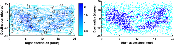
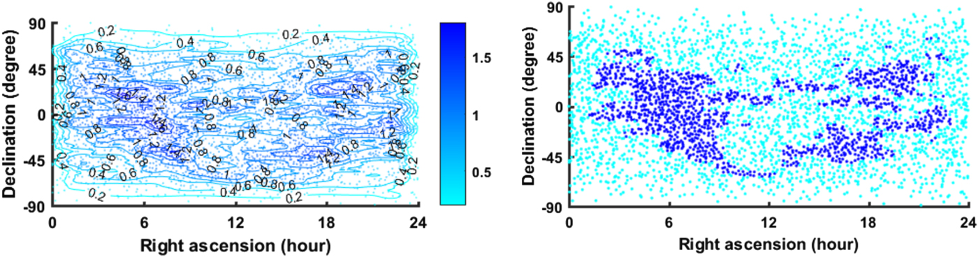
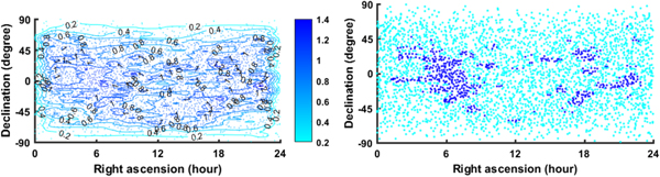
Finally, after satisfying the convergence condition of the GWKM, in order to reduce the number of stars and generate the uniform star catalogue, the brightest star near the centre of each cluster was stored and the resulting uniform catalogue was sent to the screening algorithm with the scattered data density. Following the implementation of the density determination algorithm, stars with a density higher than one were considered as non-uniform stars (blue-darker) and the rest (cyan/brighter) were selected as uniform stars. In the proposed algorithm, a density higher than one is a thinning criterion for uniformity. Figure 6 shows the output of the first step of the uniformity and density determination algorithm.

Figure 6.

The first step of the uniformity and determination of the scattered data density.

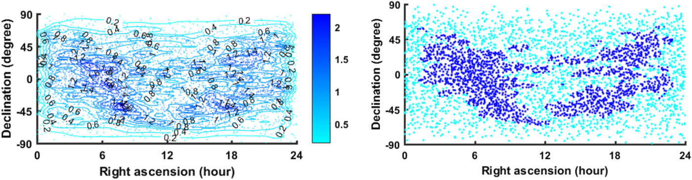
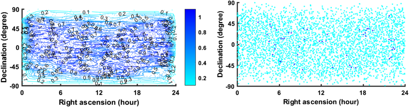
In the next step, only non-uniform stars (blue-darker) were selected and this data was entered into the uniformity process by decreasing the Delaunay triangulation resolution. Then, the uniform result obtained in this step was combined with the uniform catalogue of the previous step (cyan/brighter) and the final result was sent back to the screening algorithm. It should be noted that the decrease in the resolution of the Delaunay triangulation leads to an increase in the area of the produced triangles and thus a decrease in the resolution of the stars in the uniform catalogue. The decrease in resolution of the Delaunay triangulation is shown in Figure 2 (from right to left). Figures 7, 8 and 9 respectively show the output of the second, fifth and seventeenth step of the uniformity and density determination algorithm.

Figure 7.

The second step of the uniformity and determination of the scattered data density.

Figure 8.

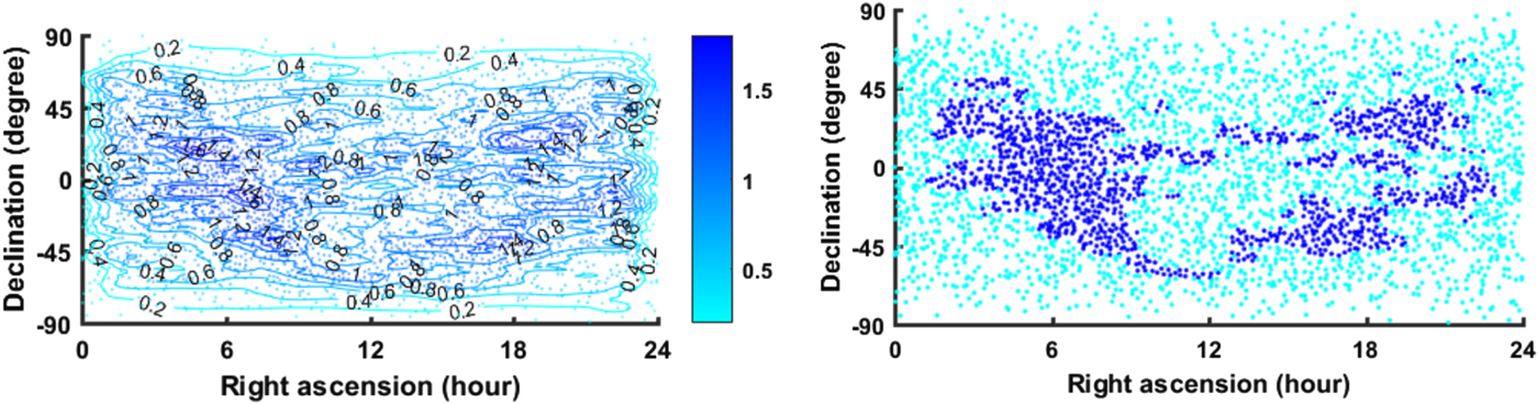
The fifth step of uniformity and determination of the scattered data density.

Figure 9.

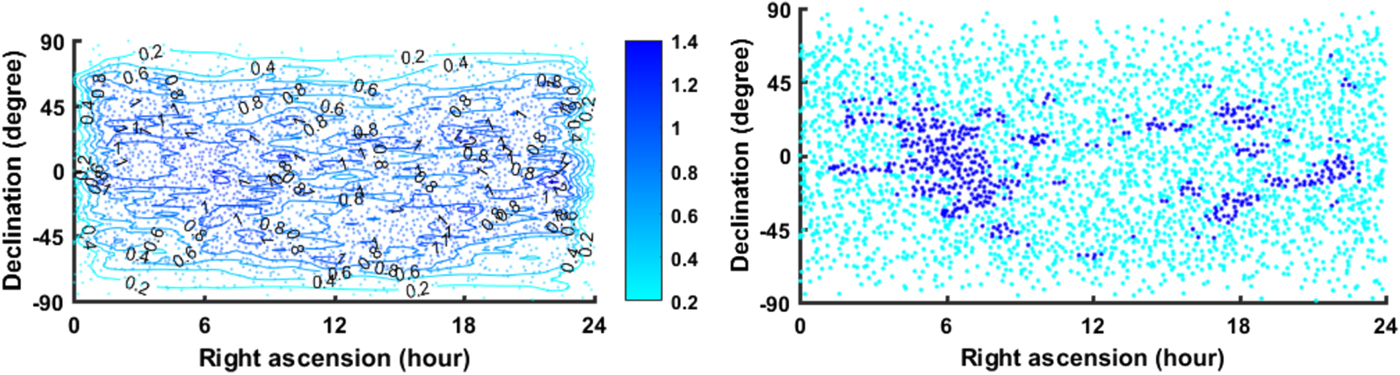
The seventeenth step of uniformity and determination of the scattered data density.

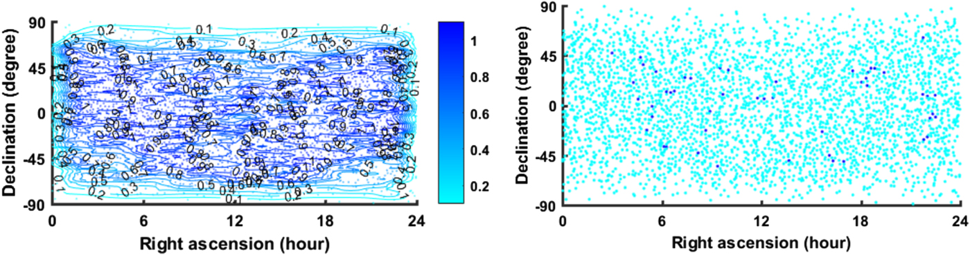
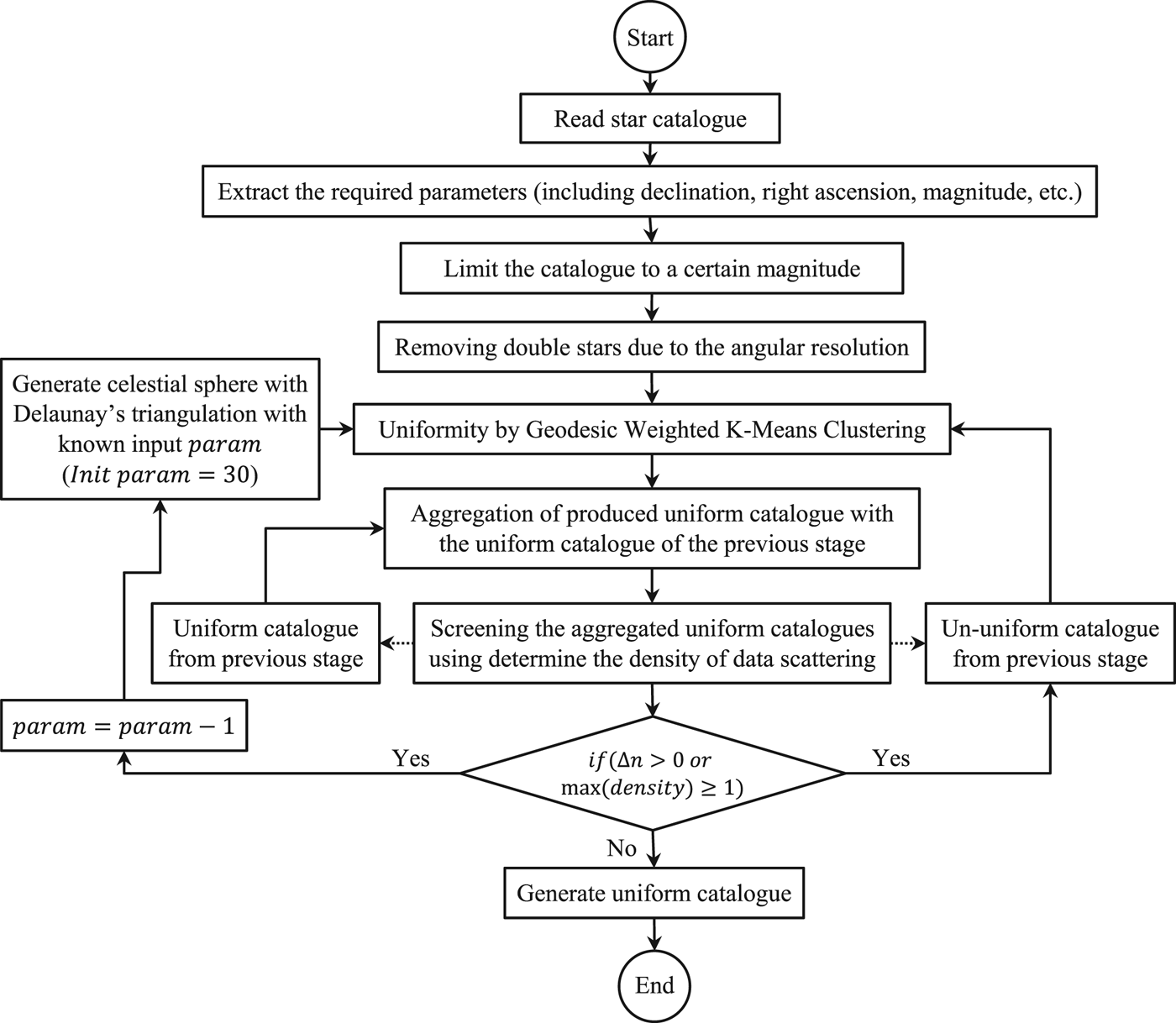
Based on the flowchart shown in Figure 10, this process continues to reduce the density of scattered data (aggregated uniform catalogue) to less than one, or the convergence of the number of non-uniform stars to a constant number.

Figure 10.

The proposed algorithm for generating the uniform catalogue from the reference catalogue.

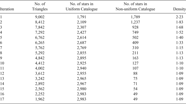
Table 2 and Figure 11 present the results of the uniformity and the final output, respectively.

Figure 11.

Uniformed catalogue with the geodesic weighted k-means clustering.

Table 2.

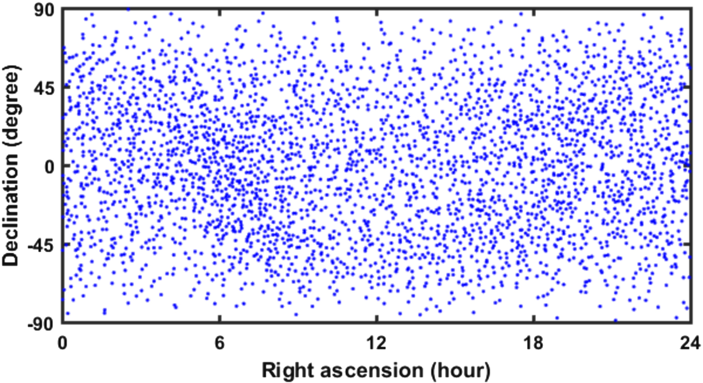
The results of the implementation of the uniformity algorithm.

As observed, in the proposed GWKM clustering method, the problem of the initial number and location of cluster centres was solved using Delaunay triangulation. Further, the problem of outlier data is solved because of the uniform distribution of points across the entire celestial sphere. The problem of determining the appropriate number of initial points (triangulation resolution), as well as the non-uniform density of stars was solved by using the algorithm of determining the scattered data density. Thus, the proposed uniformity method reduced the number of uniform catalogue stars by about 57·6% compared to the limited catalogue and reached 2,983. In Li et al. (Reference Li, Wang and Wei2018), this reduction was 32·3% (for Hipparcos reference catalogue and minimum magnitude six) and led to 3,276 guide stars in the uniform catalogue.

7. PERFORMANCE VERIFICATION

In order to investigate the effect of the proposed uniformity process on the quality of the generated uniform catalogue and observing the minimum stars required for the identification algorithm, a non-uniform catalogue (limited to a magnitude of six and the elimination of double stars – Figure 5) and generated uniform databases (Figure 11) were used to simulate the celestial sphere. This test was conducted by using star sensor simulation with an ideal pinhole model as presented in Somayehee et al. (Reference Somayehee, Nikkhah and Roshanian2018).

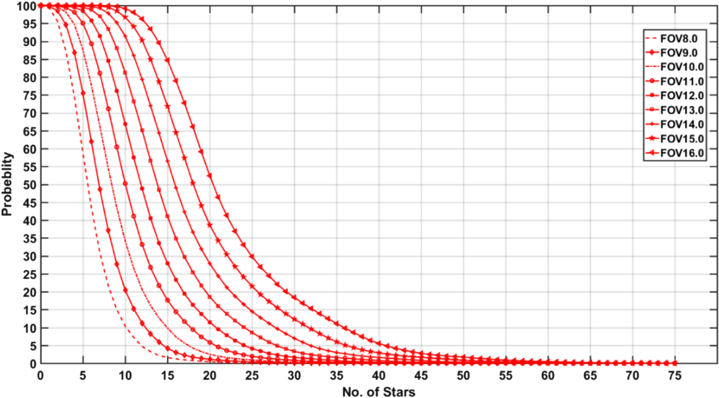
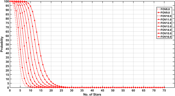
Thus, the Monte Carlo simulation was run 50,000 times for a non-uniform catalogue and the same number for the uniform databases by using random attitude and different fields of view from 8° to 16°, with a 1° step size. The probability of observing the different number of stars in each field of view was calculated and plotted, and the results are shown in Figures 12 and 13.

Figure 12.

The probability of observing a certain number of stars in different FOVs for a non-uniform catalogue (Figure 5).

Figure 13.

The probability of observing a certain number of stars in different FOVs for a GWKM uniform database (Figure 11).

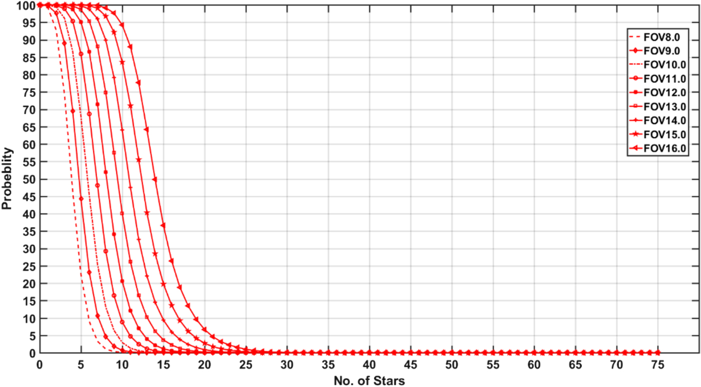
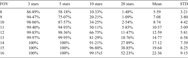
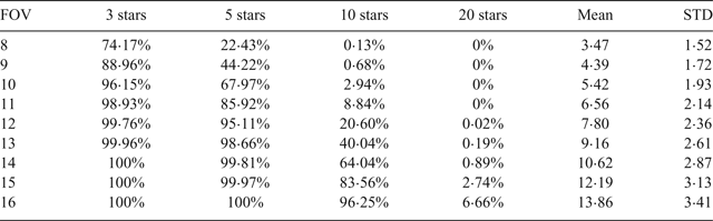
As illustrated in Figures 12 and 13, the probability of observing more than 30 stars in all possible fields of view is zero. In addition, Tables 3 and 4 present the probability of viewing three, five, more than 10 and 20 stars along with the mean and standard deviation of the observed stars in all fields of view used in the test.

Table 3.

Statistics of the Monte Carlo simulation for the non-uniform catalogue.

Table 4.

Statistics of the Monte Carlo simulation for the uniform database.

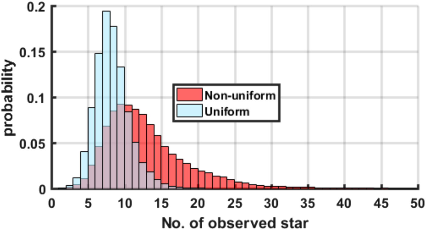
As can be seen, the proposed algorithm reduced the mean and standard deviation of observed stars. Figure 14 illustrates the probability distributions for observing the number of stars in a 12° field of view for non-uniform catalogues and a uniform database.

Figure 14.

The probability distribution for observing the number of stars in the 12° field of view (for non-uniform catalogues and uniform database).

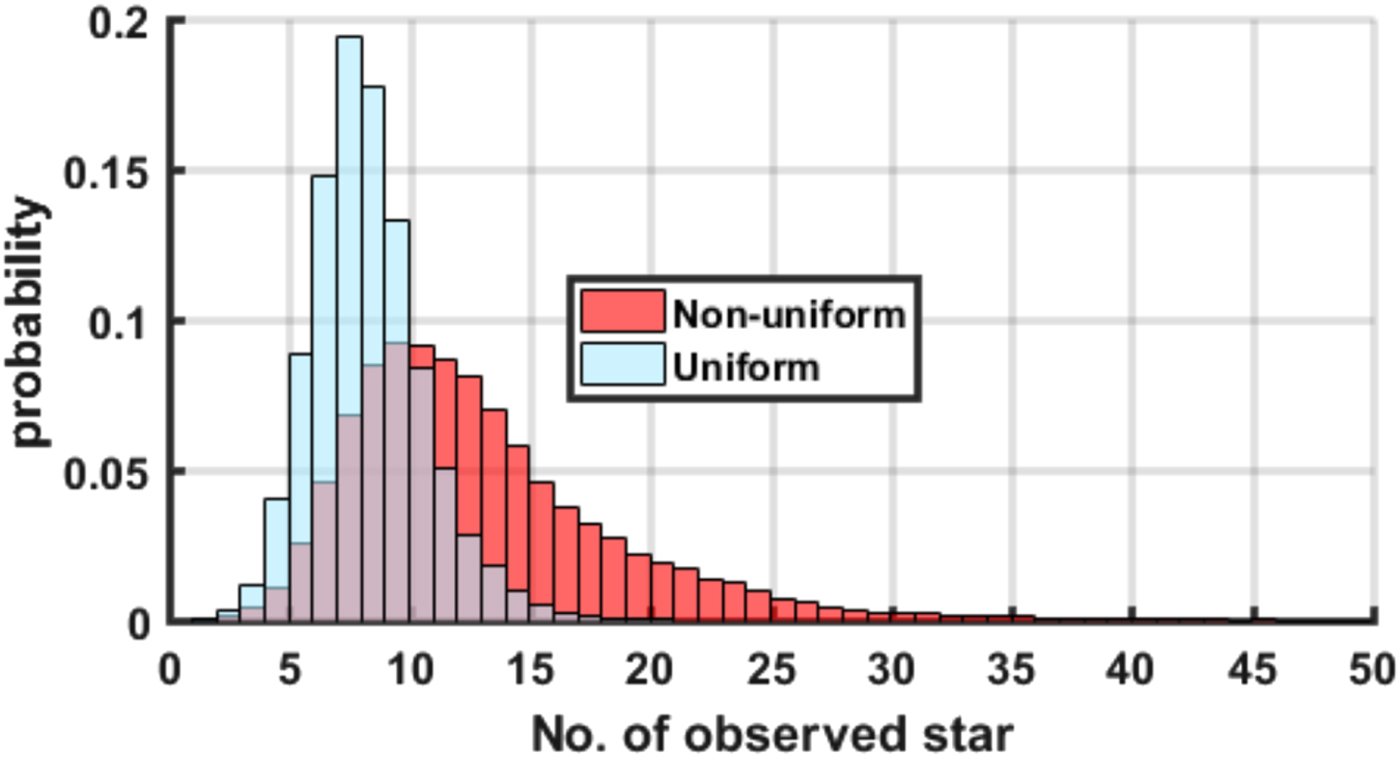
Although the use of the proposed uniformity method in the different FOV leads to a reduction in the probability of observing a certain number of stars, it significantly decreases when observing a large number of stars such as more than 10 or 20 stars in the FOV. For example, the probability of observing at least five stars in the 12° FOV of view is 98·36% for the non-uniform catalogue, while this probability decreased to 95·11% in the uniform database. This result shows a significant improvement over the results of Somayehee et al. (Reference Somayehee, Nikkhah and Roshanian2018). In this earlier work, to view five stars and more in more than 95% of cases, the required FOV should be at least 12·5°.

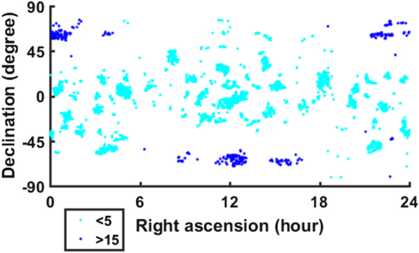
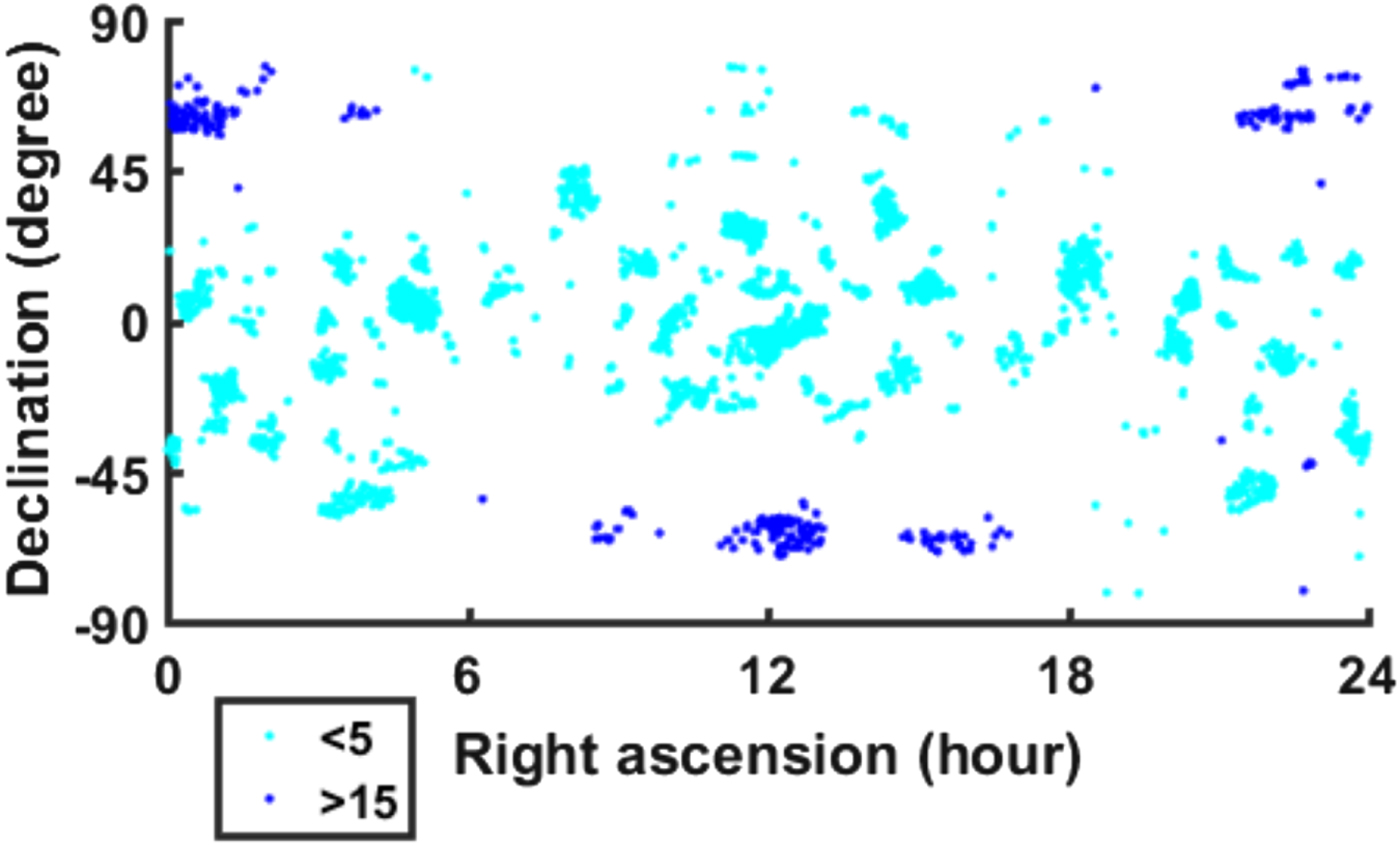
On the other hand, for a 12° FOV, the probability of observing more than 20 stars is about 11·47% in a non-uniform catalogue, while this probability decreased in the uniform database by 0·02%. It is worth mentioning, that for observing five stars in a non-uniform catalogue at a confidence level of more than 95%, there is a need for a FOV of a little more than 11°, while the required field of view is about 12° in the uniform database. Therefore, it can be concluded that the catalogue uniformity necessitates a slight increase in FOV and a change in the optical design parameters, despite the considerable advantages in reducing the size of the database and processing time, as well as increasing the reliability of the star identification algorithm. Figure 15 indicates the spatial distribution of areas with the probability of observing a different number of stars (less than five and more than 15 stars).

Figure 15.

The spatial distribution of areas with the probability of observing less and more than 15 stars.