





1. Introduction
Suspensions of elongated, rod-shaped particles at high solid volume fraction appear in many natural and industrial settings, where it is critical that their rheology and, ultimately, their fluid mechanical behaviour are well characterised (Butler & Snook Reference Butler and Snook2018). In forested areas, for instance, fallen trees and branches can accumulate on bodies of water with their structure evolving slowly and eventually forming sprawling interlocked ‘log-jam’ structures at river narrowings, negatively impacting animal habitats (Deshpande & Crosby Reference Deshpande and Crosby2019). Elsewhere, magma flows often comprise crystalline needle-like rods of much smaller size but similar aspect ratio
 $A$
that generate complex flow phenomenology and lead to rapid arrest as the material cools (Cimarelli et al. Reference Cimarelli, Costa, Mueller and Mader2011; Moitra & Gonnermann Reference Moitra and Gonnermann2015). In industry, widely employed reactive crystallisation processes critical to the manufacture of speciality chemicals generate concentrated suspensions of micrometre-sized shards or whiskers that can be well approximated as rods (Zhang & Darvell Reference Zhang and Darvell2010; Choo et al. Reference Choo, Salleh, Kok and Matori2019; Cao et al. Reference Cao, Liu, Li and Huang2022). Likewise, in paper making viscous slurries of fibres form entangled networks that give rise to non-Newtonian rheology (Derakhshandeh et al. Reference Derakhshandeh, Kerekes, Hatzikiriakos and Bennington2011; Jung et al. Reference Jung, Plumb-Reyes, Lin and Mahadevan2025). In all of these cases, the system eventually reaches sufficiently high solid volume fraction that rod–rod interactions dominate the overall stress response – that is, they are dense – and the constituent particles are large enough that diffusive motion originating from Brownian forces is significantly slower than the convective motion introduced by shearing. Additionally, the particles typically remain suspended at long times, either by neutral buoyancy with the fluid, by viscous resuspension or by support through networks of contact forces.
The basic understanding of suspension rheology has its origins in the work of Stokes (Reference Stokes1851), Einstein (Reference Einstein1911) and Batchelor & Green (Reference Batchelor and Green1972), who described how the presence of spheres enhances the viscosity under dilute and semi-dilute conditions. The extension to dense conditions is usually empirical, with the most common expression relating the suspension viscosity
 $\eta _{{s}}$
to the volume fraction
 $\phi$
being the power law
 $\eta _{{s}}\sim (1-\phi /\phi _m)^{-\varsigma }$
associated with Krieger & Dougherty (Reference Krieger and Dougherty1959). Here
 $\phi _m$
is the volume fraction at which the viscosity diverges, which is highly sensitive to microscopic details. More recently, Boyer et al. (Reference Boyer, Guazzelli and Pouliquen2011) expanded upon this by introducing a model that unifies suspensions of non-Brownian, non-attractive particles with dry granular flows. They demonstrated that, in simple shear with rate
 $\dot {\gamma }$
and imposed particle pressure
 $P$
, the macroscopic friction coefficient and the volume fraction depend only on the viscous number
 $J=\eta \dot {\gamma }/P$
, where
 $\eta$
is the liquid-phase viscosity. It follows that
 $\eta _{{s}}$
depends only on
 $\phi$
and
 $\phi _m$
, and is independent of
 $\dot {\gamma }$
. In principle this argument holds irrespective of particle shape.
For non-spherical particles, the additional degree of freedom associated with their orientation introduces complexity. In shear flows, an isolated slender rod will undergo Jeffery orbits (Jeffery Reference Jeffery1922), with period set by the shear rate, the particle aspect ratio
 $A$
and the inclination out of the flow-gradient plane. In sheared packings of dry rods, meanwhile, the time- and rod-averaged alignment is along the flow direction and makes a small angle with the streamlines (Börzsönyi et al. Reference Börzsönyi, Szabó, Törös, Wegner, Török, Somfai, Bien and Stannarius2012a). This angle decreases with increasing
 $A$
, meaning particles spend more time oriented along the flow direction. Crucially, this alignment lowers the effective instantaneous viscosity when compared with a randomly oriented assembly of the same rods at the same solids fraction (Börzsönyi et al. Reference Börzsönyi, Szabó, Wegner, Harth, Török, Somfai, Bien and Stannarius2012b). The alignment of suspended particles can be markedly different, in some cases showing orientation along the vorticity direction during large-amplitude oscillatory shear. This is thought to originate in a mechanism of collision minimisation, facilitated by confinement introduced at the walls (Franceschini et al. Reference Franceschini, Filippidi, Guazzelli and Pine2011, Reference Franceschini, Filippidi, Guazzelli and Pine2014; Snook et al. Reference Snook, Guazzelli and Butler2012). Thus, particle shape leads to interesting microstructural phenomenology with the result that, unlike for the idealised case of non-Brownian spheres, knowledge of
 $\phi$
alone is insufficient for rheological prediction.
In general, though, suspensions of rods exhibit a steady increase in
 $\eta _{{s}}$
with
 $\phi$
, as with spheres, and this effect is enhanced as
 $A$
grows (Bibbó Reference Bibbó1987; Mackaplow & Shaqfeh Reference Mackaplow and Shaqfeh1996; Ralambotiana et al. Reference Ralambotiana, Blanc and Chaouche1997; Chaouche & Koch Reference Chaouche and Koch2001; Snook et al. Reference Snook, Davidson, Butler, Pouliquen and Guazzelli2014; Tapia et al. Reference Tapia, Shaikh, Butler, Pouliquen and Guazzelli2017). Most experiments have focused on the dilute or semi-dilute regimes, up to around
 $\phi =0.2$
, especially for large-
 $A$
rods, with only limited experimental results beyond this point due to the difficulty of preparing samples and measuring the rheology in such systems (but see e.g. Tapia et al. Reference Tapia, Shaikh, Butler, Pouliquen and Guazzelli2017). As a result, the rheological properties of the dense regime, where contacts and near-contact hydrodynamics dominate, remains incompletely characterised despite its importance to the application areas mentioned above. Simulations offer a complementary approach that permits controlled exploration of
 $\phi$
,
 $A$
, orientational order and other microscopic details (for instance friction or adhesion) that are difficult to access experimentally.
There have been many attempts to simulate suspensions of rods, spanning continuum (Strand et al. Reference Strand, Kim and Karrila1987; Quiñones & Olmsted Reference Quiñones and Olmsted2025), particle-based (Mackaplow & Shaqfeh Reference Mackaplow and Shaqfeh1996; Yamane et al. Reference Yamane, Kaneda and Doi1994) and coupled particle–fluid (Khan et al. Reference Khan, More, Banaei, Brandt and Ardekani2023) approaches. Stokesian dynamics (SD) (Brady & Bossis Reference Brady and Bossis1988) is a particle-based model that includes long-range many-body hydrodynamics and short-range lubrication and has successfully been used to model dilute to semi-dilute suspensions in the limit of zero inertia (Phung et al. Reference Phung, Brady and Bossis1996; Foss & Brady Reference Foss and Brady2000; Singh & Nott Reference Singh and Nott2000; Kutteh Reference Kutteh2004). Using a simplified SD approach, Mari (Reference Mari2020) simulated suspensions of short rods, treating them as dimers formed from two overlapping spheres. Near jamming, frictionless rods align along the vorticity (rather than the flow) direction. Going beyond the overlapping spheres approach, Yamane et al. (Reference Yamane, Kaneda and Doi1994) first derived a model for the lubrication forces between rod-shaped particles, limited to normal interactions between non-parallel rod shafts (omitting parallel shafts as well as shaft–end and end–end pairs). This was later expanded by Butler & Shaqfeh (Reference Butler and Shaqfeh2002) for spherocylinders, to include interactions with the hemispherical ends of the rods. Fan et al. (Reference Fan, Phan-Thien and Zheng1998) included the non-parallel shaft–shaft term (Yamane et al. Reference Yamane, Kaneda and Doi1994) when simulating the motion of rigid, non-Brownian particles modelled as cylinders in a sheared suspension, including both short- and long-range interactions. Doing so they reproduced the dependence of
 $\eta _{{s}}$
on
 $\phi$
and
 $A$
within the dilute to semi-dilute regime, in agreement with experimental data (although at a high computational cost). More broadly, for large
 $\phi$
where interparticle interactions dominate, fully resolving the many contacts and lubrication interactions between rods with SD can become prohibitively expensive (Durlofsky et al. Reference Durlofsky, Brady and Bossis1987) due to computationally expensive matrix inversions required to obtain particle velocities.
An alternative particle-based technique to study the dense regime is the discrete element method (DEM), originally developed for dry granular materials (Cundall & Strack Reference Cundall and Strack1979). Here the zero-inertia constraint is relaxed, and particle trajectories are updated directly following Newton’s second law, allowing the use of much cheaper velocity-Verlet timestepping algorithms. This approach has been used widely for modelling both spherical and non-spherical particles (Plimpton Reference Plimpton1995; Trulsson Reference Trulsson2021; Yousefian & Trulsson Reference Yousefian and Trulsson2022; Zhang & Menon Reference Zhang and Menon2025; Bilotto et al. Reference Bilotto, Trulsson and Molinari2025), and its variants are becoming a mainstay of granular suspension modelling (Gallier et al. Reference Gallier, Lemaire, Peters and Lobry2014; Dong & Trulsson Reference Dong and Trulsson2020; Ge & Brandt Reference Ge and Brandt2020; More & Ardekani Reference More and Ardekani2021; Ness Reference Ness2023). There is an extensive literature on such models applied to dry granular rods, which are most commonly described as chains of spheres (Guo et al. Reference Guo, Wassgren, Ketterhagen, Hancock, James and Curtis2012; Nan et al. Reference Nan, Wang, Liu and Tang2015; Pol et al. Reference Pol, Artoni and Richard2023). Following this approach, rods are predicted to align with their principal axes at a small angle to the flow direction, leading to shear-induced nematic order consistent with experimental observation (Guo et al. Reference Guo, Wassgren, Hancock, Ketterhagen and Curtis2015; Börzsönyi et al. Reference Börzsönyi, Szabó, Törös, Wegner, Török, Somfai, Bien and Stannarius2012a,Reference Börzsönyi, Szabó, Wegner, Harth, Török, Somfai, Bien and Stannarius
b). Similar models have also reproduced frictional fibres jamming at high volume fraction, forming a dense contact network (Guo et al. Reference Guo, Wassgren, Hancock, Ketterhagen and Curtis2015). Other DEM studies have modelled rods directly as ellipsoids (Yousefian & Trulsson Reference Yousefian and Trulsson2022; Bilotto et al. Reference Bilotto, Trulsson and Molinari2025), cylinders (Berzi et al. Reference Berzi, Thai-Quang, Guo and Curtis2016; Bilotto et al. Reference Bilotto, Trulsson and Molinari2025) or spherocylinders (Nath & Heussinger Reference Nath and Heussinger2019) and together begin to reveal how particle shape and friction affect the alignment of particles and bulk rheology. Collectively, these works show that velocity fluctuations follow the kinetic theory prediction up to a critical packing, demonstrating that granular gas models can be applicable beyond spheres (Berzi et al. Reference Berzi, Buettner and Curtis2022). They further show that frictional rods shear-thicken at
 $\phi = 0.54{-}0.59$
, just below the jamming point at
 $\phi _m$
, with larger
 $A$
associated with a stronger viscosity increase, and frictionless systems showing only shear thinning (Nath & Heussinger Reference Nath and Heussinger2019). Long (
 $A = 4$
) and flat (
 $A = 0.25$
) cylinders were found to align with the shear direction (with frictional systems having weaker induced order due to frictional torques generating relative rotations between particles), whereas the directors of the near-spherical cylinders (
 $A = 0.8{-}1.0$
) remained disordered (Berzi et al. Reference Berzi, Thai-Quang, Guo and Curtis2016, Reference Berzi, Buettner and Curtis2022; Nath & Heussinger Reference Nath and Heussinger2019). More recently, these models have been applied to suspensions, with Anzivino et al. (Reference Anzivino, Ness, Moussa and Zaccone2024) simulating systems of frictionless rod–sphere mixtures in suspension, finding that adding short rods reduces the mixture viscosity, whereas adding long rods increases it. These and other particle-based simulation studies highlight that anisotropic particles can greatly modify the rheology compared with spheres, but they also reveal limitations. Most models for elongated particles in the literature either treat rods as chains of spheres or idealise their interactions, often without the necessary hydrodynamic forces needed to simulate suspensions.
In this paper we present a particle-based simulation for dense suspensions of non-bendy, non-Brownian spherocylinders that borrows elements from the works mentioned above to produce a model that balances a faithful rendering of the dominant microscopic physics with computational tractability. Alongside frictional particle contact forces, fluid drag and shear-induced lift, we adapt the lubrication forces of Yamane et al. (Reference Yamane, Kaneda and Doi1994) and Butler & Shaqfeh (Reference Butler and Shaqfeh2002) by developing a scheme that avoids discontinuities when traversing particle-pair configurations. We track the rod trajectories using a conventional DEM algorithm complemented by a novel dynamic time-step calculation, operating in a regime where particle inertia is present but negligible. For suspensions of spheres, models containing these microscopic physics (Trulsson et al. Reference Trulsson, Andreotti and Claudin2012; Cheal & Ness Reference Cheal and Ness2018; Seto & Giusteri Reference Seto and Giusteri2018) have proven instrumental in corroborating and extending the rheological model proposed by Boyer et al. (Reference Boyer, Guazzelli and Pouliquen2011). Our model described in the following seeks to significantly extend this understanding to the broad class of suspensions of rod-shaped particles. Using the model, we advance the fundamental understanding of the rheology of suspensions of granular rods by demonstrating (i) the dependence of the viscosity
 $\eta _{{s}}$
on the volume fraction
 $\phi$
(spanning
 $\phi \approx 0$
to
 $\phi _m$
) and particle aspect ratio (spanning
 $A=1$
to
 $20$
) and (ii) the complex relation between
 $\phi$
,
 $A$
and the particle alignment, measured using the orientational order parameter. This sets the scene for future studies that map, for instance, the full dependence of
 $\phi _m$
on the microstructural details, the relation between
 $\phi$
,
 $A$
and the normal stresses and the behaviour under inhomogeneous conditions, all of which are crucial for a full fluid mechanical description of dense granular rod suspensions.
Particle-based simulation of suspensions of sheared granular spherocylindrical rods. (a) A render of a typical simulation for aspect ratio
 $A = 5$
, solid volume fraction
 $\phi = 0.3$
, with
 $N=1000$
particles coloured according to their radii with
 $R$
in white and
 $1.4R$
in blue. The terms present in the equation of motion of the particles are (b) single-body hydrodynamics comprising drag, lift and torque, governed by the imposed linear velocity profile sketched in red; (c) repulsive contact forces between overlapping pairs, labelled here to illustrate terms present in the interaction detection algorithm used to find pairwise contacts; (d) lubrication forces between neighbouring particles, calculated using a blending approach to incorporate end–end, end–shaft and shaft–shaft interactions. The various values labelled in (c,d) are defined in the main text.

Figure 1. Long description
Panel A: A render of a simulation showing a dense collection of elongated, rod-shaped particles with varying radii, colored in white and blue. Panel B: A schematic depicting single-body hydrodynamics, including drag, lift, and torque forces acting on a rod-shaped particle within an imposed linear velocity profile. Panel C: A detailed diagram illustrating repulsive contact forces between overlapping pairs of rod-shaped particles, with various terms labeled to show interaction detection. Panel D: A diagram showing lubrication forces between neighboring particles, calculated using a blending approach to incorporate end-end, end-shaft, and shaft-shaft interactions, with various values labeled.
2. Simulation method
2.1. Equations of motion of suspended granular rods
We model particles as cylinders with hemispherical caps (figure 1) hereafter referred to as spherocylinders. This geometry resembles rod-shaped particles but simplifies interaction detection compared with alternatives such as cylinders (Gan & Yu Reference Gan and Yu2020) or spheroids (Lin & Han Reference Lin and Han2002), although it is limited to prolate particles. Each particle
 $i$
is defined by its centre of mass
 $\boldsymbol{r}_i$
, radius
 $R_i$
(the same for the shaft and hemispherical caps), shaft length
 $L_i$
and direction unit vector
 $\boldsymbol{u}_i$
. We define the aspect ratio as
 $A=({L+2R})/{2R}$
(so spheres have
 $A=1$
). The translational motion of particle
 $i$
is described by the following equation:
 \begin{align} m_i \frac {{\rm d} \boldsymbol{v}_i}{{\rm d}t} = \sum _{\kern-1pt j}\boldsymbol{F}_{\!{C}, {\textit{ij}}} + \sum _k\boldsymbol{F}_{{\!L}, \textit{ik}} + \boldsymbol{F}_{\!{H}, i}, \end{align}
where
 $m_i$
is the mass of the particle,
 $\boldsymbol{v}_i$
is its translational velocity and
 $t$
is time. The forces included in the model are pairwise contact forces
 $\boldsymbol{F}_{\!{C}, {\textit{ij}}}$
acting between particle
 $i$
and its contacting neighbours
 $j$
, pairwise lubrication forces
 $\boldsymbol{F}_{{\!L}, \textit{ik}}$
acting between particle
 $i$
and its near-neighbours
 $k$
and single-body hydrodynamic forces
 $\boldsymbol{F}_{\!{H}, i}$
. The rotational motion of each particle is similarly governed by
 \begin{align} \boldsymbol{I_i} \frac {{\rm d} \boldsymbol{\omega }_i}{{\rm d}t} = \sum _{\kern-1pt j}\boldsymbol{T}_{\!{C}, {\textit{ij}}} + \sum _k\boldsymbol{T}_{{L}, \textit{ik}} + \boldsymbol{T}_{\!{H}, i}, \end{align}
where
 $\boldsymbol{I_i}$
is a diagonal matrix denoting the mass moment of inertia of particle
 $i$
,
 $\boldsymbol{\omega }_i$
is its angular velocity and
 $\boldsymbol{T}$
the torque acting on it, which similarly has contributions from contacts, lubrication and single-body hydrodynamics labelled equivalently to the forces. For a pairwise interaction between particles
 $i$
and
 $j$
, the torque on particle
 $i$
is calculated as
 $\boldsymbol{T_i} = \boldsymbol{F}_{{\textit{ij}}} \times \boldsymbol{\ell }_{{\textit{ij}}}$
, where
 $\boldsymbol{\ell }_{{\textit{ij}}}$
is the moment arm from the centre of mass
 $\boldsymbol{r}_i$
to the point of interaction along rod
 $i$
and
 $\boldsymbol{F}_{{\textit{ij}}}$
is the relevant force term. After summing the forces and torques on each particle, details of which are described in turn below, the equations of motion are integrated numerically using a standard implementation of the velocity-Verlet algorithm.
2.2. Single-body hydrodynamic forces
Suspended neutrally buoyant particles experience hydrodynamic forces when their velocity differs from that of their surrounding fluid. Due to their anisotropic shape, suspended rods experience orientation-dependent driving, so that the forces
 $\boldsymbol{F}_{\!{H}}$
have contributions from both drag
 $\boldsymbol{F}_{\!{H,D}}$
and lift
 $\boldsymbol{F}_{\!{H,L}}$
and there also exists a torque contribution
 $\boldsymbol{T}_{\!{H}}$
. These are illustrated in figure 1(b). Although numerical simulations have sought to model the hydrodynamic forces on spherocylinders for limited aspect ratios and finite Reynolds number (Chéron et al. Reference Chéron, Evrard and van Wachem2024; Feng & Michaelides Reference Feng and Michaelides2023), a generalised analytical solution does not yet exist for the drag forces experienced in Stokes flow, the regime of interest here. In lieu of this, we adopt the result for prolate spheroids, which exists in the literature in analytical form and represents a reasonable approximation for spherocylindrical rods, especially at higher aspect ratios (Happel & Brenner Reference Happel and Brenner2012). The following summarises the work of Zhang et al. (Reference Zhang, Ahmadi, Fan and McLaughlin2001). Here single-hatted variables are defined in the particle frame of reference, which has origin at the centre of mass of the particle
 $\boldsymbol{r}_i$
and
 $z$
axis aligned with the principal axis of the particle
 $\boldsymbol{u}_i$
. Unhatted variables are defined in the laboratory frame of reference. The drag force experienced by axisymmetric particles was derived by Brenner (Reference Brenner1963) and takes a similar form to the Stokes drag on a sphere (Stokes Reference Stokes1851):
 \begin{align} \boldsymbol{F}_{\!{H,D},i} = \boldsymbol{K} \pi \eta R_i \boldsymbol{\cdot }(\boldsymbol{v}_{{f},i} - \boldsymbol{v}_i)\mathrm{.} \end{align}
Here
 $\eta$
is the liquid-phase viscosity,
 $\boldsymbol{v}_{{f},i}$
is the fluid velocity at the centre of mass of particle
 $i$
assuming the velocity profile to be linear across the domain and
 $\boldsymbol{{K}}$
is a geometric resistance tensor that takes into account the orientation of the particle with respect to the background fluid velocity field. The geometric resistance tensor is first defined as a diagonal tensor in the particle frame of reference (Fan & Ahmadi Reference Fan and Ahmadi1995) as
 \begin{align} \hat {k}_{\hat {x}\hat {x}} &= \hat {k}_{\hat {y}\hat {y}} = \frac {16(A^2 - 1)}{\left [ (2A^2 - 3) \frac {\ln {\left ( A + \sqrt {A^2 - 1}\right )}}{\sqrt {A^2 - 1}} \right ] + A}, \\[-12pt] \nonumber \end{align}
 \begin{align} \hat {k}_{\hat {z}\hat {z}} &= \frac {8(A^2 - 1)}{\left [ (2A^2 - 1) \frac {\ln {\left ( A + \sqrt {A^2 - 1}\right )}}{\sqrt {A^2 - 1}} \right ] - A}. \\[-12pt] \nonumber \end{align}
Here
 $\hat {k}_{\hat {z}\hat {z}}$
corresponds to the principal axis along the length of a rod, while the degenerate terms
 $\hat {k}_{\hat {x}\hat {x}}$
and
 $\hat {k}_{\hat {y}\hat {y}}$
represent the short axes. This can then be transformed to the laboratory frame of reference (
 $\boldsymbol{{K}} = \boldsymbol{{M}}^{-1} \boldsymbol{\hat {{K}}} \boldsymbol{{M}}$
) using the transformation matrix
 $\boldsymbol{M}$
:
 \begin{align} \boldsymbol{M} = \begin{bmatrix} \cos \xi \cos \kappa - \cos \theta \sin \kappa \sin \xi & \cos \xi \sin \kappa + \cos \theta \cos \kappa \sin \xi & \sin \xi \sin \theta \\[4pt] -\sin \xi \cos \kappa - \cos \theta \sin \kappa \cos \xi & -\sin \xi \sin \kappa + \cos \theta \cos \kappa \cos \xi & \cos \xi \sin \theta \\[4pt] \sin \theta \sin \kappa & -\sin \theta \cos \kappa & \cos \theta \end{bmatrix} \!, \end{align}
where
 $\xi$
,
 $\kappa$
and
 $\theta$
are the Euler angles between the particle director
 $\boldsymbol{u}_i$
and the laboratory frame. For axisymmetric particles degeneracy about the principal axis allows us to set
 $\xi =0$
so that
 $\boldsymbol{M}$
simplifies to
 \begin{align} \boldsymbol{M} = \begin{bmatrix} \cos \kappa & \sin \kappa & 0 \\[4pt] - \cos \theta \sin \kappa & \cos \theta \cos \kappa & \sin \theta \\[4pt] \sin \theta \sin \kappa & -\sin \theta \cos \kappa & \cos \theta \end{bmatrix} \!. \end{align}
In addition to the drag force, a particle may experience shear-induced lift
 $\boldsymbol{F}_{\!{H,L}}$
in the presence of a velocity profile. Lift is an inertial effect so is included in our model for completeness. As will be explained in § 2.4.3, however, our simulation parameters are set such that particle inertia is negligible so that in practice lift forces are significantly smaller than all other forces in the system. The lift acting on an arbitrary shaped particle (Harper & Chang Reference Harper and Chang1968) with a fluid velocity gradient
 ${{\rm d}{v}_x}/{{\rm d}z}$
in the
 $z$
direction is
 \begin{align} \boldsymbol{F}_{\!{H,L},i} = \pi ^2 R_i^2\sqrt {{\eta \rho _{{F}}}} \frac {{\rm d}{v}_x / {\rm d} z}{\sqrt {|{\rm d} {v}_x / {\rm d} z|}}(\boldsymbol{{K}} \boldsymbol{\cdot }\boldsymbol{L}_{{M}} \boldsymbol{\cdot }\boldsymbol{{K}}) \boldsymbol{\cdot }(\boldsymbol{v}_{{f},i} - \boldsymbol{v}_i), \end{align}
where
 $\rho _{{F}}$
is the fluid density and
 $\boldsymbol{L}_{{M}}$
is the coefficient matrix of the lift tensor for arbitrary shapes (Harper & Chang Reference Harper and Chang1968) and widely used for spheroids and spherocylinders (Wang et al. Reference Wang, Yu, Luo, Xia and Zong2018; Chéron et al. Reference Chéron, Evrard and van Wachem2024; Zhang et al. Reference Zhang, Ahmadi, Fan and McLaughlin2001; Cui et al. Reference Cui, Decker, Janocha, Körner and Weigand2018):
 \begin{align} \boldsymbol{L}_{{M}} = \begin{bmatrix} 0.0501 & 0.0329 & 0.00 \\[4pt] 0.0182 & 0.0173 & 0.00 \\[4pt] 0.00 & 0.00 & 0.0373 \end{bmatrix} \!. \end{align}
The hydrodynamic torque on an ellipsoidal particle in a linear shear flow is given by Jeffery (Reference Jeffery1922), wherein the total torque is composed of a viscous drag component that resists rotation and an additional shear-induced component arising from the imposed velocity gradient:
 \begin{align} \boldsymbol{T}_{\!{H}, x} &= \frac {16 \pi \eta R^3 A}{3 \left (\beta _0 + A^2 \gamma _0 \right )} \big [ \big(1 - A^2 \big) d_{\hat {z}\hat {y}} + \big(1 + A^2\big) \big(w_{\hat {z}\hat {y}} - \omega _{\hat {x}} \big) \big ], \\[-12pt] \nonumber \end{align}
 \begin{align} \boldsymbol{T}_{\!{H}, y} &= \frac {16 \pi \eta R^3 A}{3 \left (\alpha _0 + A^2 \gamma _0 \right )} \big[ \big(A^2 - 1 \big) d_{\hat {x}\hat {z}} + \big(1 + A^2 \big) \big(w_{\hat {x}\hat {z}} - \omega _{\hat {y}} \big) \big ], \\[-12pt] \nonumber \end{align}
 \begin{align} \boldsymbol{T}_{\!{H}, z} &= \frac {32 \pi \eta R^3 A}{3 \left (\alpha _0 + \beta _0 \right )} \big(w_{\hat {y}\hat {x}} - \omega _{\hat {z}} \big), \\[10pt] \nonumber \end{align}
where
 $\omega$
as before is the angular velocity of the particle (with
 $i$
subscripts dropped for clarity). Additionally,
 $d$
are elements of the deformation rate tensor
 $\boldsymbol{\hat {D}} = ({1}/{2}) ( \boldsymbol{\nabla }v + (\boldsymbol{\nabla }v)^T )$
and
 $w$
are elements of the spin tensor
 $\boldsymbol{\hat {W}} = ({1}/{2}) ( \boldsymbol{\nabla }v - (\boldsymbol{\nabla }v)^T )$
, both written in the particle frame of reference. The velocity gradient tensor, naturally expressed in the laboratory frame, can be transformed into the particle frame via
 $\hat {\boldsymbol{G}}=\boldsymbol{M}\boldsymbol{G}\boldsymbol{M}^{-1}$
.
The dimensionless parameters
 $\alpha _0$
,
 $\beta _0$
and
 $\gamma _0$
(Gallily & Cohen Reference Gallily and Cohen1979) take into account the geometry of the particles and are given by
 \begin{align} \alpha _0 = \beta _0 &= \frac {A^2}{A^2 - 1} + \frac {A}{2 (A^2 - 1)^{3/2}} \ln {\left [ \frac {A - \sqrt {A^2 - 1}}{A + \sqrt {A^2 - 1}} \right ]}, \\[-12pt] \nonumber \end{align}
 \begin{align} \gamma _0 &= -\frac {2}{A^2 - 1} - \frac {A}{(A^2 - 1)^{3/2}} \ln {\left [ \frac {A - \sqrt {A^2 - 1}}{A + \sqrt {A^2 - 1}} \right ]}. \\[10pt] \nonumber \end{align}
This shear-induced torque captures the characteristic rotational behaviour of elongated particles in viscous flows, reproducing the Jeffery orbits observed in real suspensions (Jeffery Reference Jeffery1922).
2.3. Pairwise interaction forces
2.3.1. Interaction detection
Before introducing the contact and lubrication forces, we first describe our algorithm for detecting whether neighbouring particles are close enough to be interacting. Spherocylinders have both a long and short dimension, meaning the minimum distance between their surfaces cannot be determined from the positions of their centres of mass. Instead, detecting a contact requires computing the shortest distance between the two rod spines and comparing it with the sum of their radii. To do this, we implement the method described by Vega & Lago (Reference Vega and Lago1994) for rods of arbitrary radii (
 $R_i$
,
 $R_{\kern-1pt j}$
) although alternative methods have been used (Pournin et al. Reference Pournin, Weber, Tsukahara, Ferrez, Ramaioli and Liebling2005; Angklomkleaw et al. Reference Angklomkleaw, Srinophakun and Tengpavadee2019). In general, points along the spines of rods
 $i$
and
 $j$
can be defined as
 \begin{align} \boldsymbol{\vartheta }_i &= \boldsymbol{r}_i + \lambda \frac {L_i}{2} \boldsymbol{u}_i, \\[-12pt] \nonumber \end{align}
 \begin{align} \boldsymbol{\vartheta }_{\kern-1pt j} &= \boldsymbol{r}_{\kern-1pt j} + \psi \frac {L_{\kern-1pt j}}{2} \boldsymbol{u}_{\kern-1pt j}, \\[10pt] \nonumber \end{align}
where
 $\lambda$
and
 $\psi$
are fractions of the half-length of a rod that signify the distances along the spine from the centres of mass
 $\boldsymbol{r}_i$
and
 $\boldsymbol{r}_{\kern-1pt j}$
, respectively. These distances are sketched in figure 1(c). The values of
 $\psi$
and
 $\lambda$
are
 $[-1, 1]$
for finite-length rods. The vector between these points
 $\boldsymbol{r}$
is then
 \begin{align} \boldsymbol{r} = \boldsymbol{\vartheta }_{\kern-1pt j} - \boldsymbol{\vartheta }_i = \boldsymbol{r}_{{\textit{ij}}} + \psi \frac {L_{\kern-1pt j}}{2} \boldsymbol{u}_{\kern-1pt j} - \lambda \frac {L_i}{2} \boldsymbol{u}_i, \end{align}
where
 $\boldsymbol{r}_{{\textit{ij}}} = \boldsymbol{r}_{\kern-1pt j} - \boldsymbol{r}_i$
is the vector pointing between the two centres of mass. The values of
 $\lambda$
and
 $\psi$
that minimise
 $|\boldsymbol{r}|$
(denoted
 $\lambda '$
,
 $\psi '$
) also minimise
 $\boldsymbol{r}^2$
, and for infinitely long rods these can be found by taking the derivative of
 $\boldsymbol{r}^2$
with respect to
 $\lambda$
and
 $\psi$
, which leads to
 \begin{align} \lambda ' &= \frac {2}{L_i} \frac {(\boldsymbol{r}_{{\textit{ij}}} \boldsymbol{\cdot }\boldsymbol{u}_i) - (\boldsymbol{u}_i \boldsymbol{\cdot }\boldsymbol{u}_{\kern-1pt j})(\boldsymbol{r}_{{\textit{ij}}} \boldsymbol{\cdot }\boldsymbol{u}_{\kern-1pt j})}{1 - (\boldsymbol{u}_i \boldsymbol{\cdot }\boldsymbol{u}_{\kern-1pt j})^2}, \\[-12pt] \nonumber \end{align}
 \begin{align} \psi ' &= - \frac {2}{L_{\kern-1pt j}} \frac {(\boldsymbol{r}_{{\textit{ij}}} \boldsymbol{\cdot }\boldsymbol{u}_{\kern-1pt j}) - (\boldsymbol{u}_i \boldsymbol{\cdot }\boldsymbol{u}_{\kern-1pt j})(\boldsymbol{r}_{{\textit{ij}}} \boldsymbol{\cdot }\boldsymbol{u}_i)}{1 - (\boldsymbol{u}_i \boldsymbol{\cdot }\boldsymbol{u}_{\kern-1pt j})^2}. \\[10pt] \nonumber \end{align}
These minimising values can be
 $[-\infty , \infty ]$
. If both are
 $[-1, 1]$
then the closest point between the infinitely extended rod spines falls within the finite bounds of the actual rods and
 $\lambda '$
and
 $\psi '$
can be used directly in (2.11) to find the points of closest approach. If one of the fractions does not fall within
 $[-1, 1]$
, then an additional step is required to find the closest distance within the finite bounds of the rod. First, whichever of the two fractions is further from the limits
 $[-1, 1]$
is trimmed to be at the limit (e.g.
 $\lambda ' = -10.2$
becomes
 $\lambda '' = -1$
). This truncated value (
 $\lambda ''$
or
 $\psi ''$
) is then used to find the value of the complementary fraction (
 $\psi ''$
or
 $\lambda ''$
), again from the derivative of
 ${\boldsymbol{r}}^2$
, using the appropriate one of the following expressions:
 \begin{align} \lambda '' &= \psi '' \frac {L_{\kern-1pt j}}{2} (\boldsymbol{u}_i \boldsymbol{\cdot }\boldsymbol{u}_{\kern-1pt j}) + (\boldsymbol{r}_{{\textit{ij}}} \boldsymbol{\cdot }\boldsymbol{u}_i), \\[-12pt] \nonumber \end{align}
 \begin{align} \psi '' &= \lambda '' \frac {L_i}{2} (\boldsymbol{u}_i \boldsymbol{\cdot }\boldsymbol{u}_{\kern-1pt j}) - (\boldsymbol{r}_{{\textit{ij}}} \boldsymbol{\cdot }\boldsymbol{u}_{\kern-1pt j}). \\[10pt] \nonumber \end{align}
If the value thus obtained is within the bounds
 $[-1, 1]$
, then
 $\lambda ''$
and
 $\psi ''$
can directly replace
 $\lambda$
and
 $\psi$
in (2.11). Otherwise, the obtained value is itself trimmed to within the bounds, and can then be used.
Once
 $\boldsymbol{\vartheta }_i$
and
 $\boldsymbol{\vartheta }_{\kern-1pt j}$
are found, a determination can be made of whether two particles are interacting. Particles are in direct contact if the distance between the two closest points along their spines,
 $\boldsymbol{r}$
, is less than the sum of their radii, that is,
 $|\boldsymbol{r}| \leq R_i + R_{\kern-1pt j}$
. This is true for spherocylinders since the vector connecting the closest points on the two rods is always normal both to the spines and to the particle surfaces. The overlap between two particles is then
 $\delta _{n, {\textit{ij}}} = ( R_i + R_{\kern-1pt j} ) - |\boldsymbol{r}|$
, where the normal direction of the contact vector is given by
 $\boldsymbol{n}_{{\textit{ij}}} = \boldsymbol{r}/|\boldsymbol{r}|$
. The point of interaction
 $\boldsymbol{r}_c$
is then taken as the midpoint between the surfaces of the interacting particles.
2.3.2. Contact forces
Direct contacts between particles are modelled as Hookean with Coulombic friction, with normal and tangential components of the forces computed as follows, based on the work by Mahajan et al. (Reference Mahajan, Nijssen, Kuipers and Padding2018). The total contact force acting on particle
 $i$
is the sum of the normal
 $\boldsymbol{F}_{\!{C}, n, {\textit{ij}}}$
and tangential
 $\boldsymbol{F}_{\!{C}, t,{\textit{ij}}}$
components contributed by contacting neighbours
 $j$
:
 \begin{align} \boldsymbol{F}_{\!{C}, {\textit{ij}}} = \sum \big(\boldsymbol{F}_{\!{C}, n, {\textit{ij}}} + \boldsymbol{F}_{\!{C}, t, {\textit{ij}}} \big). \end{align}
Here the normal force is modelled as a damped spring:
 \begin{align} \boldsymbol{F}_{\!{C},n, {\textit{ij}}} = -k_n \delta _{n, {\textit{ij}}} \boldsymbol{n}_{{\textit{ij}}} + \zeta _n \boldsymbol{v}_{n, {\textit{ij}}}, \end{align}
where
 $k_n$
is the normal spring constant,
 $\boldsymbol{n}_{{\textit{ij}}}$
is the unit direction vector of the interaction as defined in the preceding section,
 $\zeta _n$
is the normal damping coefficient and recalling that
 $\delta _{n, {\textit{ij}}}$
is the scalar overlap between the contacting particles. Here
 $\boldsymbol{v}_{n, {\textit{ij}}}$
is the component of the relative velocity at the point of contact along the direction
 $\boldsymbol{n}_{{\textit{ij}}}$
, defined as
 \begin{align} \boldsymbol{v}_{{\textit{ij}}} = \boldsymbol{v}_{\kern-1pt j} - \boldsymbol{v}_i + \boldsymbol{\omega }_{\kern-1pt j} \times (\boldsymbol{r}_{c} - \boldsymbol{r}_{\kern-1pt j}) - \boldsymbol{\omega }_i \times (\boldsymbol{r}_c - \boldsymbol{r}_i). \end{align}
The normal damping coefficient (Pournin Reference Pournin2005) entering (2.16) is calculated as
 \begin{align} \zeta _n = - \frac {2 m_{\textit{eff}}}{t_c} \ln {e_n}, \end{align}
where
 $m_{{eff}}$
is the effective mass of the particle pair participating in the interaction (
 $m_{{eff}} = {m_i m_{\kern-1pt j}}/({m_i+m_{\kern-1pt j}})$
) and
 $t_c$
is the duration of the contact determined as
 \begin{align} t_c = \sqrt {\frac {m_{\textit{eff}}}{k_n} \big(\pi ^2 + \ln e_n^2 \big)}. \end{align}
Here
 $e_n$
is the normal restitution coefficient of the particle, which sets how much kinetic energy is preserved after an interaction in the absence of suspending fluid.
The tangential contact force is modelled similarly, but with the inclusion of an upper limit set by a friction coefficient
 $\mu$
and defined according to
 \begin{align} \boldsymbol{F}_{\!{C}, t, {\textit{ij}}} = \begin{cases} -k_t \boldsymbol{\delta }_{t, {\textit{ij}}} + \zeta _t \boldsymbol{v}_{t, {\textit{ij}}} & \mathrm{for}\quad |\boldsymbol{F}_{\!{C},t, {\textit{ij}}}| \leq \mu |\boldsymbol{F}_{\!{C}, n, {\textit{ij}}}|, \\[5pt] - \mu |\boldsymbol{F}_{\!{C}, n, {\textit{ij}}}| \boldsymbol{t}_{{\textit{ij}}} & \mathrm{for}\quad |\boldsymbol{F}_{\!{C},t, {\textit{ij}}}| \gt \mu |\boldsymbol{F}_{\!{C}, n,{\textit{ij}}}|, \end{cases} \end{align}
where
 $\boldsymbol{\delta }_{t, {\textit{ij}}}$
is the tangential overlap which quantifies the elastic tangential deformation of a particle since the onset of the contact and
 $k_t$
is the tangential spring constant. Here
 $\zeta _t$
is the tangential damping coefficient,
 $\boldsymbol{v}_{t, {\textit{ij}}}$
is the tangential component of the relative velocity at the point of contact and
 $\boldsymbol{t}_{{\textit{ij}}}$
is the unit vector in the direction of the static tangential force, ensuring the sliding force opposes the tangential deformation and relative motion. The quantities
 $t_c$
,
 $e_n$
and
 $e_t$
can in principle be measured from simple single-contact experiments, informing an appropriate choice for
 $k_n$
. Having specified the tangential restitution coefficient
 $e_t$
and calculated the contact time
 $t_c$
, the tangential stiffness
 $k_t$
can then be found using (Pournin Reference Pournin2005)
 \begin{align} k_t = t_c^{-2} \left ( \frac {1}{m_{\textit{eff}}} + \frac {|\boldsymbol{r}_c - \boldsymbol{r}_i|^2}{\langle I_i \rangle } + \frac {|\boldsymbol{r}_c - \boldsymbol{r}_{\kern-1pt j}|^2}{\langle I_{\kern-1pt j} \rangle } \right )^{-1} \big(\pi ^2 + \ln {e_t}^2 \big), \end{align}
where
 $\langle I_i \rangle$
is the average mass moment of inertia defined below in (2.23) and
 $e_t$
is the tangential restitution. The tangential damping coefficient
 $\zeta _t$
(Pournin Reference Pournin2005) is
 \begin{align} \zeta _t = t_c^{-1} \left ( \frac {1}{m_{\textit{eff}}} + \frac {|\boldsymbol{r}_c - \boldsymbol{r}_i|^2}{\langle I_i \rangle } + \frac {|\boldsymbol{r}_c - \boldsymbol{r}_{\kern-1pt j}|^2}{\langle I_{\kern-1pt j} \rangle } \right )^{-1} \ln {e_t}. \end{align}
For a spherocylinder the non-zero components of the mass moments of inertia
 $\boldsymbol{\hat {I}}$
, in the particle frame of reference, can be calculated (Pournin et al. Reference Pournin, Weber, Tsukahara, Ferrez, Ramaioli and Liebling2005; Constantin Reference Constantin2015) as
 \begin{align} I_{\hat {x}\hat {x}} &= I_{\hat {y}\hat {y}} = \pi \rho _{{P}} \left (\frac {1}{12} R^2 L^3 + \frac {8}{15} R^5 + \frac {1}{3} R^3 L^2+ \frac {3}{4} R^4 L\right ) \!, \\[-12pt] \nonumber \end{align}
 \begin{align} I_{\hat {z}\hat {z}} &= \pi \rho _{{P}} \left (\frac {1}{2} R^4 L + \frac {8}{15} R^5\right ) \!, \\[-12pt] \nonumber \end{align}
 \begin{align} \langle I \rangle &= \frac {1}{3} \big(I_{\hat {x}\hat {x}} + I_{\hat {y}\hat {y}} + I_{\hat {z}\hat {z}} \big), \\[10pt] \nonumber \end{align}
where
 $\rho _{{P}}$
is the particle density. The tangential overlap
 $\boldsymbol{\delta }_{t, {\textit{ij}}}$
is obtained by integrating the relative tangential velocity between two particles over the duration of the contact:
 \begin{align} \boldsymbol{\delta }_{t, {\textit{ij}}}(t) = \int _{t_{c, 0}}^{t} \boldsymbol{v}_{t, {\textit{ij}}}\, {\rm d}t. \end{align}
Together, the normal and tangential force models described above provide a description of particle contact interactions within the simulation, capturing both damped spring forces and frictional dissipation.
2.3.3. Lubrication forces
Lubrication forces arise from short-range hydrodynamic interactions generated when two particles within a fluid move relative to each other in close proximity. These forces originate in the viscosity of the fluid in the narrow gap between the particles, opposing their relative motion. Lubrication forces become particularly important at small surface-to-surface separations
 $h$
and hence are an essential component of the equation of motion for particles in dense suspension. Importantly, the discontinuity in the curvature of spherocylinders at the end–shaft junction precludes an analytical model for the lubrication force (Janoschek et al. Reference Janoschek, Harting and Toschi2013). To address this, Butler & Shaqfeh (Reference Butler and Shaqfeh2002) proposed a modification of the Yamane et al. (Reference Yamane, Kaneda and Doi1994) model, adapting it to spherocylinders by treating the three possible interaction configurations separately, namely the shaft–shaft (SS), end–shaft (ES) and end–end (EE) interactions:
 \begin{align} \boldsymbol{F}_{{\!L,SS},{\textit{ij}}} &= -24 \frac {\eta \pi R^2}{h_{{\textit{ij}}}} \frac {A^2}{(2A + 1) \left [ \left ( A^2 + \dfrac {1}{4} \right ) |\boldsymbol{u}_i \times \boldsymbol{u}_{\kern-1pt j}|^2 + A \left ( 1 + (\boldsymbol{u}_i \boldsymbol{\cdot }\boldsymbol{u}_{\kern-1pt j})^2 \right ) \right ]^{1/2}} \boldsymbol{v}_{n, {\textit{ij}}} \boldsymbol{n}_{{\textit{ij}}}, \\[-12pt] \nonumber \end{align}
 \begin{align} \boldsymbol{F}_{{\!L,ES},{\textit{ij}}} &= - \frac {4}{\sqrt {2}} \frac {\eta \pi R^2}{h_{{\textit{ij}}}} \boldsymbol{v}_{n, {\textit{ij}}} \boldsymbol{n}_{{\textit{ij}}}, \\[-12pt] \nonumber \end{align}
 \begin{align} \boldsymbol{F}_{{\!L,EE},{\textit{ij}}} &= - \frac {3}{2} \frac {\eta \pi R^2}{h_{{\textit{ij}}}} \boldsymbol{v}_{n, {\textit{ij}}} \boldsymbol{n}_{{\textit{ij}}}, \\[10pt] \nonumber \end{align}
where
 $A$
is the aspect ratio,
 $h$
is the separation between the surfaces of particles (
 $h_{{\textit{ij}}} = |\boldsymbol{r}| - ( R_i + R_{\kern-1pt j} )$
) and
 $\eta$
is the fluid viscosity. This separate treatment of the different interaction modes leads to a discontinuity in the force when a pair of particles moves in time from one type of interaction to another, an issue that is amplified at higher aspect ratios. We resolve this by computing all three components (2.25a–2.25c) for all neighbouring pairs, but assigning weights to each term dependent on the relative position of the two particles. This requires three lengths to be defined that quantify the SS, ES and EE distances, with the importance of each force term then being inversely proportional to its associated distance. The initial SS weight is thus defined as
 $ C_{\textit{SS}} = (1/\varpi _{\textit{SS}})/(1/\varpi _{\textit{SS}}+1/\varpi _{\textit{ES}}+1/\varpi _{\textit{EE}})\mathrm{,}$
with analogous expressions for
 $C_{\textit{ES}}$
and
 $C_{\textit{EE}}$
so that by construction we have
 $C_{\textit{SS}} + C_{\textit{ES}} + C_{\textit{EE}} = 1$
. These weights contribute to the overall expression for the lubrication force as
 \begin{align} \boldsymbol{F}_{{\!L}, {\textit{ij}}} = C_{\textit{SS}} \boldsymbol{F}_{{\!L, SS}, {\textit{ij}}} + C_{\textit{ES}} \boldsymbol{F}_{{\!L, ES}, {\textit{ij}}} + C_{\textit{EE}} \boldsymbol{F}_{{\!L, EE}, {\textit{ij}}}. \end{align}
The distances
 $\varpi _{\textit{SS}}$
etc. must be defined such that the appropriate component dominates, i.e.
 $C_{\textit{EE}}$
is most influential in an end–end interaction and
 $C_{\textit{SS}}$
is most influential when rods are parallel. This is achieved by imagining the rod as split into spherical end sections with a smaller internal cylindrical shaft section. Within this representation we define the distances
 $\varpi _{\textit{EE}}=h_{\textit{EE}}+2R$
,
 $\varpi _{\textit{ES}}=h_{\textit{ES}}+R$
and
 $\varpi _{\textit{SS}}=h_{\textit{SS}}$
as sketched in figure 1(d). Here each
 $h$
term is used for the respective force calculation in (2.25), while the corresponding
 $\varpi$
term is used to set the weighting assigned to that force. This scheme alone resolves the aforementioned discontinuities, but to further improve the correction the weights can be manually adjusted to produce smoother transitions between interaction types (e.g.
 $aC_{\textit{SS}} + bC_{\textit{ES}} + cC_{\textit{EE}} = 1$
, where
 $a$
,
 $b$
and
 $c$
are manually set corrective values and within our simulations are
 $a = 0.1$
,
 $b = 1.0$
,
 $c = 5.0$
). These values are determined by considering a series of different primitive pairwise motions (i.e. particles sliding past one another along a common axis; perpendicular to one another; and so on) that involve transitions in dominance from one type of lubrication interaction to another (e.g. transitioning from shaft–shaft to shaft–end). These weight correctors are then individually adjusted until a smooth profile is produced for each case. Having obtained these profiles, we then verify that the choice of weights has minimal impact on the rheological predictions of our model. This approach is successful for aspect ratios
 $A\geq 3$
, since the middle section needs to be at minimum a sphere for the distances to be calculated. When evaluating each of the force components in (2.26), the corresponding separation
 $h_{\textit{SS}}$
etc. is used along with the average
 $R$
for interactions between particles of different sizes.
To ensure numerical stability as the gap between particle surfaces vanishes, a minimum separation is specified. This distance is defined as a fixed fraction
 $h_{\textit{min}}$
of the radii for an interacting pair, so that below separations of
 $h_{\textit{min}}(R_1+R_2)$
the separation
 $h_{{\textit{ij}}}$
used in calculations is not further decreased. Such a length scale might physically represent the size of asperities on the particle surfaces, which are not explicitly modelled here. Additionally, to reduce computational cost and avoid unphysical interactions with secondary neighbours (e.g. where particles interact through other particles) a maximum separation
 $h_{\textit{max}}$
was similarly introduced to define a point above which lubrication forces between particles are not computed. These lengths are sketched in figure 1(d).
2.4. Additional model details
2.4.1. Stress calculation
The stress within the system is calculated as the sum of the stress contributions from pairwise particle interactions
 $\boldsymbol{\sigma }_{{P}}$
, and a fluid contribution
 $\boldsymbol{\sigma }_{{F}}$
. The former is a
 $3\times 3$
tensor constructed from the moment arm
 $\boldsymbol{\ell }$
and force
 $\boldsymbol{F}$
vectors, and is defined as (Marschall & Teitel Reference Marschall and Teitel2019)
 \begin{align} \boldsymbol{\sigma }_{{P}} = -\frac {1}{V} \left ( \sum ^{N_{{C}}}\boldsymbol{\ell }_{{\textit{ij}}} \otimes \boldsymbol{F}_{\!{C}, {\textit{ij}}} + \sum ^{N_{{L}}} \boldsymbol{\ell }_{ik} \otimes \boldsymbol{F}_{{\!L}, \textit{ik}} ,\right ) \!, \end{align}
where
 $N_{{C}}$
is the number of contacts (which occur between particles
 $i$
and
 $j$
),
 $N_{{L}}$
is the number of lubrication interactions (which occur between particles
 $i$
and
 $k$
),
 $V$
is the total volume of the system and
 $\otimes$
is the outer product. In the following we consider only the shear stress, written for simplicity as
 $\sigma _{{P}}$
. Meanwhile the single-body forces generate an additional contribution to the shear stress (labelled here as
 $\sigma _{{F}}$
to denote the fluid contribution), given for spherical particles by Einstein (Reference Einstein1911) and later modified for spherocylinders by Kuhn (Reference Kuhn1933) to read
 \begin{align} {\sigma }_{{F}} = \eta \dot {\gamma } \left ( 1 + \dfrac {5}{2} \phi + \dfrac {\phi }{16} A^2\right ) \!\mathrm{,} \end{align}
where we omit higher-order terms in
 $\phi$
. This equation is strictly valid only in dilute systems, and is limited in that it does not account for particle ordering, instead assuming an isotropic and randomly distributed suspension. At the high volume fractions of interest, however, the fluid contribution becomes negligible relative to the stresses arising from particle–particle interactions. Any contribution to the fluid stress coming from particle structure, following for example Dinh & Armstrong (Reference Dinh and Armstrong1984), would not change this, and would likely be dominated by structural contributions to the stress arising from lubrication and contact forces. In the following we report the reduced shear viscosity of the suspension as
 $\eta _{{s}}=(\sigma _{{F}}+\sigma _{{P}})/\eta \dot {\gamma } = \sigma /\eta \dot {\gamma }$
.
2.4.2. Quantifying alignment
To understand the material response to flow, we characterise the microstructural arrangement of the particles borrowing insight from the Q-tensor commonly used to characterise alignment in nematic liquid crystals. We quantify the degree of collective ordering of the particles by computing the largest eigenvalue
 $S$
of the order tensor
 $\boldsymbol{T}$
, the components of which are defined as
 \begin{align} {T_{\alpha \beta }} = \left \langle \frac {3}{2} u_{i, \alpha } u_{i, \beta } - \frac {1}{2} \delta _{\alpha \beta }\right \rangle \!. \end{align}
Here
 $\alpha$
and
 $\beta$
represent the Cartesian coordinates, and angle brackets indicate averaging over all particles
 $i=1,\ldots ,N$
. This leads to the orientational order parameter
 $S$
, a scalar metric that takes values in the range
 $[0,1]$
. A value of
 $S=1$
means that the system is perfectly regularly aligned, i.e. all particles are parallel to one another, whereas a value of
 $S=0$
represents completely uncorrelated particle directors. The eigenvector
 $\boldsymbol{u}_{\textit{princ}}$
associated with
 $S$
represents the principal direction of alignment.
2.4.3. Simulation set-up and parameters
Particles governed by the above set of forces and torques are placed with initially random positions and orientations in a cubic domain consisting of periodic boundaries in the
 $x$
and
 $y$
directions and Lees–Edwards boundary conditions (Lees & Edwards Reference Lees and Edwards1972) across the
 $z$
axis. An example snapshot of the simulated system is given in figure 1(a). The latter is used to introduce a velocity difference across the domain that leads, through the imposed drag forces described above, to a linear fluid velocity profile
 $v_{{f},x}=\dot {\gamma }z$
. The minimum domain size is then two times the maximum interaction length of a particle. Here this is equal to the total length of the particle plus the additional length of influence due to the lubrication force
 $h_{\textit{max}}R$
on each end. The minimum system size is therefore
 $2R ( A + 1 + h_{\textit{max}} )$
. It is standard practice in spheres to include a bidisperse mixture of radii (typically 1:1.4) to prevent crystallisation (VanderWerf et al. Reference VanderWerf, Jin, Shattuck and O’Hern2018; O’hern Reference O’hern2002; Zhang Reference Zhang2009). For each value of
 $A$
we therefore simulated a bidisperse system comprising equal numbers of particles with radius and length ratio both set to 1:1.4. It is worth noting though that this choice has little impact on the rheology reported in the following. Indeed we found little change in the steady-state viscosity predicted by the simulation when moving from mono- to bi- to tridisperse systems.

Table 1. Long description
A table listing global parameters for simulations. The table has 10 columns and 2 rows. Column headers are R 1, R 2, R 1: R 2, ρ F, ρ P, k n, e n, e t, μ, η, h min, h max. Row 1 values are L, L, 1:1, 1, 1.5 x 10^6, 0.5, 0.5, 0.5, 15, 0.025, 0.9.

Table 2. Long description
A table with 30 rows and 5 columns. The columns are labeled N, phi, A, y-dot, and sigma fixed. The table lists simulation parameters for each test case reported in figures 26. Row 1: N, 1000; phi, 0.01; A, 5; y-dot, 0.07; sigma fixed, empty. Row 2: N, 1000; phi, 0.1; A, 5; y-dot, 0.07; sigma fixed, empty. Row 3: N, 1000; phi, 0.2; A, 5; y-dot, 0.07; sigma fixed, empty. Row 4: N, 1000; phi, 0.3; A, 5; y-dot, 0.07; sigma fixed, empty. Row 5: N, 1000; phi, 0.4; A, 5; y-dot, 0.07; sigma fixed, empty. Row 6: N, 1000; phi, 0.47; A, 5; y-dot, 0.07; sigma fixed, empty. Row 7: N, 1000; phi, 0.5; A, 5; y-dot, 0.07; sigma fixed, empty. Row 8: N, 1000; phi, 0.52; A, 5; y-dot, 0.07; sigma fixed, empty. Row 9: N, 1000; phi, 0.55; A, 5; y-dot, 0.07; sigma fixed, empty. Row 10: N, 1000; phi, 0.3; A, 5; y-dot, 0.035; sigma fixed, empty. Row 11: N, 1000; phi, 0.3; A, 5; y-dot, empty; sigma fixed, 2.5. Row 12: N, 1000; phi, 0.3; A, 5; y-dot, empty; sigma fixed, 5. Row 13: N, 1000; phi, 0.01; A, 10; y-dot, 0.07; sigma fixed, empty. Row 14: N, 1000; phi, 0.15; A, 10; y-dot, 0.07; sigma fixed, empty. Row 15: N, 1000; phi, 0.25; A, 10; y-dot, 0.07; sigma fixed, empty. Row 16: N, 1000; phi, 0.33; A, 10; y-dot, 0.07; sigma fixed, empty. Row 17: N, 1000; phi, 0.4; A, 10; y-dot, 0.07; sigma fixed, empty. Row 18: N, 1000; phi, 0.45; A, 10; y-dot, 0.07; sigma fixed, empty. Row 19: N, 1000; phi, 0.5; A, 10; y-dot, 0.07; sigma fixed, empty. Row 20: N, 1059; phi, 0.53; A, 10; y-dot, 0.07; sigma fixed, empty. Row 21: N, 1119; phi, 0.56; A, 10; y-dot, 0.07; sigma fixed, empty. Row 22: N, 1000; phi, 0.01; A, 15; y-dot, 0.07; sigma fixed, empty. Row 23: N, 1000; phi, 0.13; A, 15; y-dot, 0.07; sigma fixed, empty. Row 24: N, 1000; phi, 0.2; A, 15; y-dot, 0.07; sigma fixed, empty. Row 25: N, 1144; phi, 0.28; A, 15; y-dot, 0.07; sigma fixed, empty. Row 26: N, 1349; phi, 0.33; A, 15; y-dot, 0.07; sigma fixed, empty. Row 27: N, 1553; phi, 0.38; A, 15; y-dot, 0.07; sigma fixed, empty. Row 28: N, 1839; phi, 0.45; A, 15; y-dot, 0.07; sigma fixed, empty. Row 29: N, 2003; phi, 0.49; A, 15; y-dot, 0.07; sigma fixed, empty. Row 30: N, 2085; phi, 0.51; A, 15; y-dot, 0.07; sigma fixed, empty.
The parameters within the model are chosen such that (i) particle inertia can be considered insignificant,
 $\dot \gamma ^* \equiv \rho _{{F}} \dot {\gamma } R^2 / \eta \lt 10^{-2}$
; and (ii) rods can be assumed to be very hard,
 $\dot {\gamma } \sqrt {\rho _{{P}} R^3 / k_n} \lt 10^{-4}$
. Table 1 includes the material properties and other parameter values used throughout all of the simulations. We chose modest values of the friction coefficient and normal restitution coefficient, noting that experimentally a wide range of values both above (Mair et al. Reference Mair, Frye and Marone2002) and below (Foerster et al. Reference Foerster, Louge, Chang and Allia1994) our chosen friction coefficient
 $\mu$
are observed in similar systems. The same is true for the normal restitution coefficient
 $e_n$
(Foerster et al. Reference Foerster, Louge, Chang and Allia1994; Joseph et al. Reference Joseph, Zenit, Hunt and Rosenwinkel2001). We opted for values comfortably within the ranges found in the literature, acknowledging that they may not be representative of a specific single material. Simulations suggest that the qualitative alignment behaviour reported here is independent of the particle friction, though we defer a systematic study of the role of the friction coefficient to future work. Table 2 then gives the values that are altered for each test case. For each set of parameters presented the simulation was repeated for five realisations, each starting from a distinct initial configuration.
2.4.4. Time-step size
The equations of motion given above are integrated in time to update the particle trajectories. The discrete time step
 ${\rm d}t$
used for this integration needs to be carefully chosen to resolve all interactions while not adding unnecessarily to the computation time. To achieve this we therefore need to approximate the characteristic time scale of each interaction. The time scale associated with the contact force is the contact time
 $t_c$
(2.19). This time scale depends only on the material properties and the mass of the particles. It increases with aspect ratio but does not depend on the relative orientation of the contacting particles so is constant throughout an interaction. There is also a time scale associated with the lubrication force
 $t_{{lub}, \boldsymbol{F}}$
. This can be approximated from the term in the equation of translational motion (2.1) corresponding to the lubrication force. For simple shear we can make the assumption that the magnitude of the relative velocity between interacting particles is
 $|{\rm d}v| \sim R\dot \gamma$
. For simplicity we may also assume that
 $\boldsymbol{F}_{{\!L},{SS}}$
is the dominant component of the lubrication force, since this grows with
 $A$
. With these assumptions we can approximate the time scale of a lubrication interaction as
 \begin{align} t_{{lub}, \boldsymbol{F}, {\textit{ij}}} & \approx \frac {1}{36} \frac {\rho _{{P}} h_{\textit{SS}} R^2 \dot \gamma }{|\boldsymbol{v}_{n, {\textit{ij}}}|\eta } \frac {(2A+1)(3A-1)}{A^2} \nonumber \\ & \qquad \left [ \left ( A^2 + \frac {1}{4} \right ) |\boldsymbol{u}_i \times \boldsymbol{u}_{\kern-1pt j}|^2 + A \big ( 1 + (\boldsymbol{u}_i \boldsymbol{\cdot }\boldsymbol{u}_{\kern-1pt j})^2 \big ) \right ]^{1/2}. \end{align}
Here, unlike the contact time, we have a time scale that is configuration-dependent and therefore changes over the course of an interaction. Moreover, unlike
 $t_c$
the lubrication time scale decreases with increasing aspect ratio. For elongated particles, the time scale for the force differs notably from that of the torque due to the large moment arm. The time scale associated with the lubrication torque
 $t_{{lub}, \boldsymbol{T}}$
can be approximated from the equation of rotational motion for the lubrication torque (2.2). For simple shear we can make the assumption that
 $|{\rm d}\omega | \approx \dot \gamma$
. As
 $\boldsymbol{T} = \boldsymbol{F} \times \boldsymbol{\ell }$
and assuming
 $|\boldsymbol{\ell }| \approx 0.5 L$
, we can use the approximation
 $|\boldsymbol{T}_{\textit{lub}}| \approx 0.5 L |\boldsymbol{F}_{{lub}, {SS}}|$
. The smallest component of
 $\boldsymbol{\hat {I}}$
is
 $I_{\hat {z}\hat {z}}$
for any aspect ratio and will lead to the limiting (smallest) time scale. With these assumptions we can approximate the time scale of the lubrication torque as
 \begin{align} t_{{lub}, \boldsymbol{T}, {\textit{ij}}} & \approx \frac {1}{360} \frac {\rho _{{P}} h_{\textit{SS}} R^2 \dot \gamma }{|\boldsymbol{v}_{n,{\textit{ij}}}| \eta } \frac {(2A+1)(15A-7)}{A^2(A-1)} \nonumber \\ & \qquad \left [ \left ( A^2 + \frac {1}{4} \right ) |\boldsymbol{u}_i \times \boldsymbol{u}_{\kern-1pt j}|^2 + A \big ( 1 + (\boldsymbol{u}_i \boldsymbol{\cdot }\boldsymbol{u}_{\kern-1pt j})^2 \big ) \right ]^{1/2}. \end{align}
Again we have a time scale that changes over the course of an interaction and that now scales approximately with
 $1/A^2$
. The value of
 ${\rm d}t$
for the subsequent time step is then chosen as the smallest of these time scales, which we determined dynamically by inserting the actual values of
 $h_{\textit{SS}}$
,
 $\boldsymbol{v}_{n,{\textit{ij}}}$
,
 $\boldsymbol{u}_i$
and
 $\boldsymbol{u}_{\kern-1pt j}$
for each interaction into (2.19), (2.30) and (2.31). This ensures that
 ${\rm d}t$
is always small enough to resolve ongoing interactions but never smaller than it needs to be, allowing for faster simulations.
Results of prerequisite calculations and diagnostic simulations used to determine parameter values. (a) Shown by solid lines are the characteristic time scales associated with contact and lubrication interactions, defined in (2.19), (2.32) and (2.33), while the area shaded in green highlights the range of dynamically adjusted time-step sizes
 ${\rm d}t$
that were used during the simulations. (b) Example plots of the rescaled steady-state velocity profiles, demonstrating that the desired linear profiles, specified through the imposed shear rate
 $\dot {\gamma }$
, are achieved. Shown are (i)
 $A=5$
,
 $\phi =0.1$
,
 $\dot \gamma ^*=0.007$
; (ii)
 $A=5$
,
 $\phi =0.5$
,
 $\dot \gamma ^*=0.007$
; (iii)
 $A=5$
,
 $\phi =0.3$
,
 $\dot \gamma ^*=0.0035$
; (iv)
 $A=5$
,
 $\phi =0.3$
,
 $\sigma _{\textit{fixed}} = 2.5$
[M L
 $^{-1}$
T
 $^{-2}$
] (
 $\dot \gamma ^*_{{avg}} = 0.004$
). (c) Demonstration of the shear stress control algorithm described in the text, showing transients of (i) the shear rate
 $\dot {\gamma }^*$
and (ii) the shear stress
 $\sigma$
rescaled by its set point values, for
 $\sigma _{\textit{fixed}}=\{2.5,5\}$
[M L
 $^{-1}$
T
 $^{-2}$
] (leading to
 $\dot \gamma ^*_{{avg}}$
= {0.004, 0.008}).

Figure 2. Long description
Panel A: A line graph shows characteristic time scales associated with contact and lubrication interactions as a function of aspect ratio. The x-axis represents the aspect ratio, and the y-axis represents the characteristic time in seconds. Three lines represent different time scales: contact time, lubrication time with a specific force, and lubrication time with another specific force. The area shaded in green highlights the range of dynamically adjusted time-step sizes used during the simulations. Panel B: Four subplots show rescaled steady-state velocity profiles. Each subplot has the position on the y-axis and velocity on the x-axis, demonstrating linear profiles achieved through imposed shear rates. Panel C: Two line graphs demonstrate the shear stress control algorithm. The first graph shows the shear rate over time, and the second graph shows the shear stress rescaled by its set point values over time. The x-axis represents strain, and the y-axis represents shear rate and shear stress, respectively. Different lines represent different shear rate set points.
Alternatively we can calculate a static value of
 ${\rm d}t$
by estimating the largest force or torque present when hydrodynamics dominates. For the lubrication interactions this occurs when two parallel rods interact at their minimum distance. In this configuration we can assume that
 $h_{\textit{SS}} = Rh_{\textit{min}}$
,
 $\boldsymbol{u}_i \times \boldsymbol{u}_{\kern-1pt j} = 0$
and
 $\boldsymbol{u}_i \boldsymbol{\cdot }\boldsymbol{u}_{\kern-1pt j} = 1$
. For simple shear we can additionally assume
 $\boldsymbol{v}_{n, {\textit{ij}}} = AR \dot {\gamma }$
. (This latter assumption will likely break down at higher volume fractions, where relative velocity is governed by contact forces (set by
 $k_n$
) rather than the fluid flow (set by
 $\eta$
), leading to a smaller time scale than that calculated.) Substituting these assumptions into (2.30) and (2.31) we get
 \begin{align} t_{{lub}, \boldsymbol{F}} \approx \frac {\sqrt {2}}{36} \frac {\rho _{{P}} h_{\textit{min}} R^2}{\eta } \frac {(2A+1)(3A-1)}{A^{5/2}}, \end{align}
 \begin{align} t_{{lub}, \boldsymbol{T}} \approx \frac {\sqrt {2}}{360} \frac {\rho _{{P}} h_{\textit{min}} R^2}{\eta } \frac {(2A+1)(15A-7)}{A^{5/2}(A-1)}. \end{align}
These time scales are plotted as functions of
 $A$
in figure 2(a) along with a shaded area denoting the range of actual time scales (obtained via (2.30) and (2.31)) used in each simulation.
2.4.5. System control modes
As described in § 2.2, the fluid velocity profile
 $\boldsymbol{v}_{{f}}(z)$
determines the single-body hydrodynamic forces on each particle. Throughout we prescribe a linear velocity profile by specifying a spatially invariant value of the gradient as
 $\dot {\gamma }=\partial v_{{f,x}}/\partial z$
. The simulation can impose this shear rate under two modes. In the first, we simply prescribe a fixed value of
 $\dot {\gamma }$
and run the dynamics. In the second, we seek to model an imposed shear stress rather than an imposed shear rate. To do so, at each time step
 $t$
we calculate the overall shear stress in the system as
 $\sigma _t$
, and compare it with a specified set point shear stress
 $\sigma _{\textit{fixed}}$
. The offset is then used to adjust the imposed shear rate at the next time step
 $\dot {\gamma }_{t+\Delta t}$
(introducing a gain parameter
 $K_p$
) according to
 \begin{align} \dot {\gamma }_{t+\Delta t} = \dot {\gamma }_{t} + \frac {\sigma _{\textit{fixed}} - \sigma _{t}}{\sigma _{\textit{fixed}}} K_p\mathrm{.} \end{align}
Setting
 $K_p\approx 10^{-3}\dot {\gamma }$
, and having verified that this does not introduce any unwanted transients or periodicity in the results, this control scheme keeps the overall shear stress close to the set point value.
Example velocity profiles generated by binning particle velocities along
 $z$
are plotted in figure 2(b), demonstrating that the shear rate is kept close to the one prescribed, irrespective of the volume fraction, shear rate or simulation mode (shear rate versus shear stress control). The performance of the stress controller for fixed shear stresses = {2.5, 5} [M L
 $^{-1}$
T
 $^{-2}$
] (
 $\dot \gamma ^*_{{avg}}$
= {0.004, 0.008}) is shown in figure 2(c). The set point stress is closely maintained, showing an average error of
 $\lt 1 \,\%$
once reaching the set point.
3. Results and discussion
3.1. Effect of volume fraction and aspect ratio on suspension viscosity
We simulated aspect ratios
 $A=\{1,5, 10, 15,20\}$
to cover a broad range of particle shape (figure 3). Results for
 $A=1$
were obtained using a separate sphere-only model with equivalent physics (Ness Reference Ness2023; Li et al. Reference Li, Royer and Ness2024). For each aspect ratio we explored a range of volume fractions spanning from
 $\phi =0.01$
up to sufficiently high values to approach the jamming point, which appears to decrease with
 $A$
(Tapia et al. Reference Tapia, Shaikh, Butler, Pouliquen and Guazzelli2017). Transient and steady-state viscosity data for each of these simulations are reported in figure 4.
Simulation snapshots of the initial configurations of granular rod suspensions prior to shearing. Shown are systems at
 $\dot {\gamma }t=0$
, with (a)
 $A=5, \phi =0.3$
; (b)
 $A=10, \phi = 0.33$
; (c)
 $A=15, \phi = 0.33$
; (d)
 $A=20, \phi = 0.33$
. The particles are coloured based on radius with
 $R=1$
particles coloured white and
 $R=1.4$
particles coloured blue.

Figure 3. Long description
Panel A: A 3D simulation snapshot showing a dense configuration of granular rods with a volume fraction of 0.15. The rods are colored based on radius, with smaller rods in white and larger rods in blue. Panel B: A 3D simulation snapshot showing a dense configuration of granular rods with a volume fraction of 0.25. The rods are colored based on radius, with smaller rods in white and larger rods in blue. Panel C: A 3D simulation snapshot showing a dense configuration of granular rods with a volume fraction of 0.35. The rods are colored based on radius, with smaller rods in white and larger rods in blue. Panel D: A 3D simulation snapshot showing a dense configuration of granular rods with a volume fraction of 0.45. The rods are colored based on radius, with smaller rods in white and larger rods in blue.
Simulation results showing the viscosity
 $\eta _{{s}}$
of granular rod suspensions under simple shear flow. (a) Typical transients of the suspension viscosity
 $\eta _{{s}}$
plotted against accumulated strain
 $\dot {\gamma }t$
for aspect ratio
 $A=5$
at various volume fractions
 $\phi$
, measured under a fixed shear rate of
 $\dot \gamma ^* = 0.007$
. Thinner lines show results for each individual realisation. (b) The dependence of the steady-state suspension viscosity (obtained by averaging the transient data over strains
 $\dot {\gamma }t\gt 20$
) on the volume fraction
 $\phi$
for aspect ratios
 $A=\{1,5,10,15, 20\}$
. Data for
 $A=1$
(i.e. spheres) are obtained from a separate model with equivalent physics (Ness Reference Ness2023; Li et al. Reference Li, Royer and Ness2024). Shown in the solid grey line is the expression
 $\eta _{{s}}=\iota (1-\phi /\phi _m)^{-\varsigma }$
, with
 $\phi _m=0.57$
,
 $\varsigma =0.97$
and
 $\iota =1.2$
. (c) The transient suspension viscosity for
 $\phi =0.3$
and
 $A=5$
, comparing fixed shear rate and fixed shear stress control modes to demonstrate their equivalence and the rate independence of our model. (d) Individual contributing components of the suspension viscosity for
 $A=5$
, measured as a function of
 $\phi$
. Included are the normal and tangential contact forces, the lubrication force and the contributions from single-body hydrodynamics. All of the results presented represent averages taken over five realisations, each starting from distinct initial configurations.

Figure 4. Long description
Panel A: A line graph shows the viscosity of granular rod suspensions plotted against accumulated strain for various volume fractions at a fixed shear rate. Thinner lines represent individual realizations. Panel B: A scatter plot illustrates the steady-state suspension viscosity as a function of volume fraction for different aspect ratios. A solid grey line represents a specific expression. Panel C: Another line graph compares the transient suspension viscosity for different shear rates and control modes. Panel D: A line graph displays the individual contributing components of the suspension viscosity as a function of volume fraction, including normal and tangential contact forces, lubrication force, and single-body hydrodynamics contributions.
In the transients
 $\eta _{{s}}(\dot {\gamma }t)$
for particles with
 $A=5$
(figure 4
a), there is an initial spike in the viscosity occurring at the onset of shear around
 $\dot {\gamma }t=2$
. Comparing this transient to that of the alignment (figure 6
a, discussed later), it appears that the material has a short-lived higher viscosity associated with the initial random distribution of particle orientations. This subsides once the particles start to align. Thereafter the viscosity falls and remains fluctuating around a steady-state value at large
 $\dot {\gamma }t$
. Notably, the size of the initial spike in
 $\eta _{{s}}$
relative to the steady-state value is a growing function of
 $\phi$
. This implies that the viscosity of the unsheared material may diverge more quickly with
 $\phi$
than the steady-state viscosity, suggesting microstructural dependence of the jamming point
 $\phi _m$
. The strain scale needed to reach steady state also grows with
 $\phi$
. The viscosity at large strain increases systematically with increasing
 $\phi$
, consistent with a large body of experimental work on non-Brownian suspensions (Guazzelli & Pouliquen Reference Guazzelli and Pouliquen2018).
Dense suspensions of granular rods under shear, showing example snapshots of the steady-state alignment obtained at
 $\dot {\gamma }t=200$
for each aspect ratio. Shown are the same cases as figure 3 with (a)
 $A=5, \phi =0.3$
; (b)
 $A=10, \phi = 0.33$
; (c)
 $A=15, \phi = 0.33$
; (d)
 $A=20, \phi = 0.33$
. Red arrows and line sketched on the lower left coordinate system illustrate the directions of flow
 $x$
and velocity gradient
 $z$
, while the colour bar (common to all panels) represents the
 $x$
component of the unit director
 $\boldsymbol{u}$
of each rod, with blue indicating perfect alignment along
 $x$
.

Figure 5. Long description
Panel A: A 3D visualization of rod-shaped particles with a high aspect ratio. The particles are mostly aligned in the direction of flow, indicated by blue color. A red arrow and line illustrate the flow and velocity gradient directions. Panel B: A similar 3D visualization with particles of a different aspect ratio, showing a different alignment pattern. Panel C: Another 3D visualization with particles of a different aspect ratio, showing a more uniform alignment. Panel D: A 3D visualization with particles of a different aspect ratio, showing a more disordered alignment. The color bar indicates the component of the unit director of each rod, with blue indicating perfect alignment along the flow direction.
Simulation results showing the alignment of granular rods in suspension under simple shear flow. (a) Transients of the orientational order parameter
 $S$
for
 $A=5$
and a range of volume fractions
 $\phi$
with the inset showing the period of rotation of isolated rods (
 $\phi \to 0$
) under simple shear flow at angles to the flow-gradient (
 $xz$
) plane = {
 $0^\circ$
,
 $30^\circ$
,
 $60^\circ$
}. (b) The steady states are plotted against volume fraction
 $\phi$
, additionally showing results for
 $A=\{10,15,20\}$
. (c) The steady states of the angle
 $\varphi _{{h}}$
between the projection onto the flow-vorticity (
 $xy$
) plane of the principal direction of alignment obtained via (2.29), and the flow direction
 $x$
. (d) The angle
 $\varphi _{{v}}$
between the projection onto the flow-gradient (
 $xz$
) plane of the principal direction of alignment and the flow direction
 $x$
. The sketch in the inset of (c) shows the definitions of
 $\varphi _{{h}}$
and
 $\varphi _{{v}}$
. All of the results presented represent averages taken over five realisations, each starting from distinct initial configurations.

This trend of increasing viscosity with volume fraction is observed for all aspect ratios (figure 4
b). In all cases the curves follow approximately the power law
 $\eta _{{s}}\sim (1-\phi /\phi _m)^{-\varsigma }$
at large
 $\phi$
, with the example shown in figure 4(b) for
 $A=5$
having
 $\phi _m=0.57$
and
 $\varsigma =0.97$
. Similar fits for the other curves (not plotted) are poorer, but suggest
 $\phi _m \approx \{0.59,0.49,0.41\}$
for
 $A=\{10,15,20\}$
. The features of the viscosity, namely the increase with respect to
 $\phi$
and the general variation of
 $\phi _m$
with
 $A$
, are qualitatively consistent with experiment (Mueller et al. Reference Mueller, Llewellin and Mader2011; Tapia et al. Reference Tapia, Shaikh, Butler, Pouliquen and Guazzelli2017). At the microstructural level, particles of higher aspect ratio can, for a given volume fraction, reach further into their neighbouring packing and can thus interact with more neighbours. They can therefore reach the critical number of contacts required for mechanical stability at lower
 $\phi$
, explaining the relation between
 $\phi _m$
and
 $A$
. In our results we see a very similar jamming point for the three lowest-aspect-ratio particles
 $A=\{1,5,10\}$
. This is likely due to the very high degree of alignment (figure 6
b, discussed later) in these cases, meaning that the number of contacts is not being affected by the length (i.e. two perfectly aligned
 $A=5$
rods would be roughly equivalent to one
 $A=10$
rod). The higher-aspect-ratio rods experience much greater torques meaning they are constantly pushed out of this alignment and so their length continues to play a key role in their jamming point. Additionally, higher-aspect-ratio particles contribute a greater stress to the fluid component (via (2.28)) adding further to their increased viscosity at a given
 $\phi$
. We defer a comprehensive quantification and analysis of the jamming point and its relation to aspect ratio and particle alignment to a future study.
To verify the rate independence of our model we ran simulations across both modes of operation, exploring a range of fixed shear rates and fixed shear stresses. Representative results for
 $A=5$
and
 $\phi =0.3$
(figure 4
c) demonstrate that although the precise details of the transients differ, the major features of the mechanical response are robust. Importantly, the steady-state viscosity measured by averaging the transient over large strains is independent of the shear rate. Thus the viscosity divergences reported in figure 4(b) are rate-independent, consistent with the canonical framework of Boyer et al. (Reference Boyer, Guazzelli and Pouliquen2011) for granular suspensions.
Decomposing the viscosity into its contributions from each of the force terms detailed above, we find a crossover in dominant microphysics occurring at intermediate
 $\phi$
. Again taking
 $A=5$
as a representative example, we plot in figure 4(d) the viscosity contributions from contact (normal and tangential) and lubrication forces as well as the fluid stress (2.28) as functions of
 $\phi$
. Here we see that the contact forces become negligible at small
 $\phi$
and instead the dominant contribution to the viscosity comes from the fluid component of the stress and secondarily from lubrication interactions. As
 $\phi$
increases the contact components steadily rise and eventually dominate at
 $\phi \approx 0.5$
. The lubrication forces increase more slowly with
 $\phi$
and plateau beyond this point. The value of the plateau is likely governed in part by our choice of
 $h_{\textit{min}}$
, which prevents the lubrication forces from diverging at particle contacts. Above
 $\phi =0.5$
contacts dominate, with the normal component exceeding the tangential one, and their ratio likely governed by our choice of friction coefficient
 $\mu =0.5$
.
3.2. Effect of volume fraction and aspect ratio on particle alignment
Shown in figure 5 are snapshots of simulations across
 $A$
illustrating the microstructural arrangements obtained after large strain. In general we see that particles appear to strongly align along the flow direction. We quantify these microstructural features using the order parameter
 $S$
defined above. Additionally, we report two angles:
 $\varphi _{{h}}$
, the angle formed between the flow direction
 $x$
and the projection onto the flow-vorticity (
 $xy$
) plane of the eigenvector
 $\boldsymbol{u}_{\textit{princ}}$
associated with
 $S$
; and
 $\varphi _{{v}}$
, the angle formed between the flow direction
 $x$
and the projection onto the flow-gradient (
 $xz$
) plane of
 $\boldsymbol{u}_{\textit{princ}}$
. Transients in system order
 $S$
for
 $A=5$
are shown in figure 6(a) for a range of
 $\phi$
. In all cases there is, at small
 $\dot {\gamma }t$
, an initial increase in
 $S$
from the random initial state with
 $S\approx 0$
, implying a tendency towards alignment along the flow direction. The strain over which this occurs maps onto that over which the viscosity was reported to initially spike in figure 4. This initial increase in order is followed by a slower evolution of
 $S$
with strain until steady states are reached. Notably, at
 $\phi =0.01$
there is oscillatory behaviour in
 $S$
at large strain, indicating that the packing is sparse enough to permit Jeffery-like orbits leading to periodically evolving alignment. We verified that the period of the evolution in
 $S$
is indeed consistent with the expected Jeffery orbits by separately simulating isolated rods in shear flow and measuring their alignment relative to the flow direction. Doing so systematically for three inclinations out of the flow-gradient (
 $xz$
) plane, we obtain the transients plotted in the inset of figure 6(a). The periods of these isolated cases follow closely that of the sheared suspension at
 $\phi =0.01$
, albeit with extrema in the inset varying across the full range of
 $S$
while those in the main panel of figure 6(a) are more tightly bound around
 $S\approx 0.35$
. Similar periodicity is initially evident at
 $\phi =0.1$
, before dissipating at larger strains.
Computing the time-averaged values of
 $S$
over
 $\dot {\gamma }t\gt 200$
(figure 6
b), we see that there is a range of
 $\phi$
for which
 $S$
sharply increases, spanning approximately
 $\phi =0.01{-}0.2$
for
 $A=5$
. At larger
 $\phi$
we see that
 $S$
maintains its very high order but does not increase any further. Further increasing
 $\phi$
then leads to a reduction in this steady-state order. This indicates that the particles in the system become frustrated and are no longer as able to get into or maintain strong alignment with each other. The same phenomenology in the ordering is observed for all other aspect ratios.
In addition to the extent of alignment, it is important to characterise the direction of alignment. The average alignment of the system in the
 $xy$
plane
 $\varphi _{{h}}$
is shown in figure 6(c). Here an angle of
 $0^\circ$
corresponds to particles pointing along the direction of flow, whereas an angle of
 $90^\circ$
would correspond to particles pointing into the vorticity direction. In all cases the angle is
 $\approx 0^\circ$
with the
 $x$
axis, indicating that the particles are preferentially aligning along the flow direction in a manner reported previously for sheared dry granular matter (Börzsönyi et al. Reference Börzsönyi, Szabó, Törös, Wegner, Török, Somfai, Bien and Stannarius2012a). At very low volume fractions
 $\phi =0.01$
there is some deviation from zero, likely because these systems are not very well aligned (
 $S=0.3{-}0.5$
) and do not have many contacts capable of adjusting a particle’s trajectory, meaning that some particles will remain aligned along other directions executing kayaking-like orbits. This flow alignment is seen for all aspect ratios.
Shown in figure 6(d) is the average inclination angle of the system
 $\varphi _{{v}}$
, which takes values of
 $0^\circ$
for particles pointing along the flow direction and
 $90^\circ$
for particles pointing along the gradient direction. Similar to the trend seen in
 $S$
we see a range of
 $\phi$
for which
 $\varphi _{{v}}$
increases, spanning
 $\phi =0.01{-}0.4$
, a larger range than
 $S$
. This positive angle with the flow direction has again been previously reported for similar systems (Börzsönyi et al. Reference Börzsönyi, Szabó, Törös, Wegner, Török, Somfai, Bien and Stannarius2012a). Past this point, we see that the inclination angle begins to decrease, corresponding with (and likely a consequence of) the decrease seen in
 $S$
. A similar trend is seen for the other aspect ratios. However, as
 $A$
is increased, the maximum
 $\varphi _{{v}}$
decreases and occurs at lower
 $\phi$
. This appears as a flattening of the curve and suggests that at sufficiently high aspect ratio there will be negligible inclination.
4. Conclusion and future outlook
We have developed and implemented a numerical model containing a minimal set of physics describing dense suspensions of rod-shaped particles undergoing shear flow. The model incorporates standard forms for the contact, drag and lift forces, and modified lubrication forces that resolve a prior discontinuity. It is accelerated by a novel dynamic scheme for computing the time step. Predictions of the viscosity reveal a strong increase with the solid volume fraction, which we varied across a broad range from
 $\phi =0.01$
to values approaching the jamming point
 $\phi _m$
. This jamming point, at which the viscosity diverges, decreases with aspect ratio in the range
 $A=5$
to
 $20$
, consistent with experimental observation. Measurements of the shear-induced order show flow direction alignment increasing up to a threshold volume fraction before slightly decreasing, a phenomenon seen for each aspect ratio. Our model makes possible many future lines of study directly relevant to fluid mechanical problems in engineering applications, for instance the effect of particle–particle friction coefficient on the viscosity and microstructure; the role of polydispersity both in the radius and aspect ratio of the particles; and the behaviour close to the jamming transition and its dependence on the particle alignment. It also offers the opportunity to study other flow types such as pressure-imposed flow (Etcheverry et al. Reference Etcheverry, Forterre and Metzger2023) as well as nonlinear velocity or stress profiles, adapting ideas introduced recently for suspensions of spheres (Saitoh & Tighe Reference Saitoh and Tighe2019; Bhowmik & Ness Reference Bhowmik and Ness2025). More broadly it can be used to study problems at the intersection of jammed entangled granular matter (Bhosale et al. Reference Bhosale, Weiner, Butler, Kim, Gazzola and King2022) and dense-suspension rheology (Brown et al. Reference Brown, Zhang, Forman, Maynor, Betts, DeSimone and Jaeger2011).
Acknowledgements
The authors thank J. Butler, E. Shaqfeh, J. Brady, H. Evans, T. Shendruk, D. Hodgson, J. Richards, J. Thijssen, B. Goddard and D. Berzi for useful discussions.
Funding
A.D. acknowledges financial support from Syngenta. C.N. acknowledges support from the Royal Academy of Engineering under the Research Fellowship scheme, the Leverhulme Trust under Research Project Grant RPG-2022-095, and the Engineering and Physical Sciences Research Council (EPSRC) Impact Acceleration Account EP/X525698/1. G.M. acknowledges financial support from NBIC/BBSRC/UKRI under Grant No. BB/R012415/1.
Declaration of interests
The authors report no conflict of interest.
Data availability statement
Our data and simulation code are available at https://doi.org/10.7488/ds/8194.

 A=5
 ϕ=0.3
 N=1000
 R
 1.4R

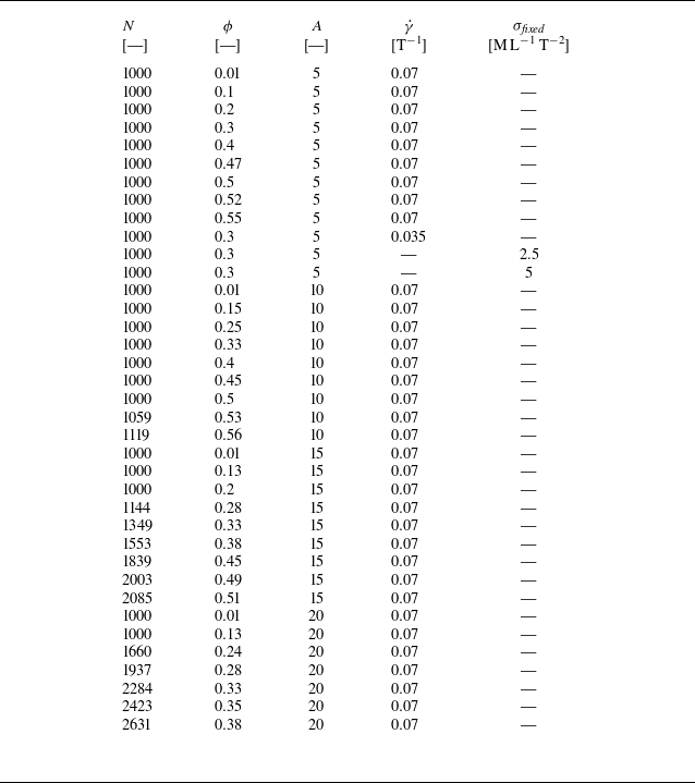

 dt
 γ˙
 A=5
 ϕ=0.1
 γ˙∗=0.007
 A=5
 ϕ=0.5
 γ˙∗=0.007
 A=5
 ϕ=0.3
 γ˙∗=0.0035
 A=5
 ϕ=0.3
 σfixed=2.5
 −1
 −2
 γ˙avg∗=0.004
 γ˙∗
 σ
 σfixed={2.5,5}
 −1
 −2
 γ˙avg∗

 γ˙t=0
 A=5,ϕ=0.3
 A=10,ϕ=0.33
 A=15,ϕ=0.33
 A=20,ϕ=0.33
 R=1
 R=1.4

 ηs
 ηs
 γ˙t
 A=5
 ϕ
 γ˙∗=0.007
 γ˙t>20
 ϕ
 A={1,5,10,15,20}
 A=1
 ηs=ι(1−ϕ/ϕm)−ς
 ϕm=0.57
 ς=0.97
 ι=1.2
 ϕ=0.3
 A=5
 A=5
 ϕ

 γ˙t=200
 A=5,ϕ=0.3
 A=10,ϕ=0.33
 A=15,ϕ=0.33
 A=20,ϕ=0.33
 x
 z
 x
 u
 x

 S
 A=5
 ϕ
 ϕ→0
 xz
 0∘
 30∘
 60∘
 ϕ
 A={10,15,20}
 φh
 xy
 x
 φv
 xz
 x
 φh
 φv

 Open access

