

I. Introduction
Products or assets are often endowed with a set of characteristics. Although the characteristics of the product usually do not have explicit prices, changes in the bundle of characteristics cause the price of the product or asset to change. Sherwin Rosen (Reference Rosen1974) built a structural model that assumed a spatial equilibrium in characteristics' space between producers and consumers, such that the hedonic price of a characteristic equaled both the consumer's marginal rate of substitution and the producer's marginal rate of transformation. Such a model allowed the implicit hedonic prices of product characteristics or attributes to be recovered by regressing product prices on characteristics. Over time, the hedonic price model has been widely adapted and refined, especially in the area of real estate, where observed house prices can be used to infer not only the values of the private characteristics of the house, such as the number of square feet, but also the values of the public good and neighborhood characteristics, such as environmental amenities and school quality. However, more than five decades of research has found that producers are not always efficient (Charnes, Cooper, and Rhodes, Reference Charnes, Cooper and Rhodes1978; Farrell, Reference Farrell1957).
In this paper we outline a method that can be used to recover hedonic prices of product or asset characteristics even when producers are technically inefficient and produce inside their technological frontier. Our method uses the directional input distance function to represent the value/characteristics space of an asset. Directional distance functions were developed by Chambers, Chung, and Färe (Reference Chambers, Chung and Färe1996, Reference Chambers, Chung and Färe1998) by adapting Luenberger's (Reference Luenberger1992, Reference Luenberger1995) benefit function. Related to directional distance functions are Shephard (Reference Shephard1953, Reference Shephard1970) distance functions, which are a special case of directional distance functions. The Shephard input and output distance functions scale inputs/outputs to an isoquant/production possibility frontier and can be used to infer the marginal rate of substitution between inputs or the marginal rate of transformation between outputs. Shephard input and output distance functions are most often estimated using a translog functional form. In contrast, Chambers (Reference Chambers, Färe, Grosskopf and Russell1998) shows that the quadratic function is more suitable for fitting directional distance functions. In addition, the quadratic form can handle data sets where one or more observations have one or more inputs/outputs that equal zero, whereas a translog function requires data to be transformed for use with observations with zeros for inputs or outputs.
Previous research by English, Grosskopf, Hayes, and Yaisawarng (Reference English, Grosskopf, Hayes and Yaisawarng1993) used Shephard output distance functions to estimate the shadow (hedonic) prices of unpriced outputs using the marginal rate of transformation and one observed output price. Färe, Grosskopf, Roland, and Weber (Reference Färe, Grosskopf, Roland and Weber2009) used the Shephard input distance function to price the property right associated with owning a Norwegian license to farm salmon. Other research by Färe, Grosskopf, and Weber (Reference Färe, Grosskopf and Weber2001) used directional distance functions to recover the shadow prices of the characteristics of sites overseen by the Missouri Department of Conservation. However, when the researcher has knowledge about the price of the bundle of characteristics but not the price of a single characteristic, the shadow pricing methods can allow recovery of the marginal rates of substitution or transformation but not the implicit equilibrium prices of the characteristics.
To circumvent the problem of unobservable characteristic prices, we exploit the duality between the cost function and the input characteristic distance function. Given the price of the bundle of characteristics and the quantities of the characteristics, we recover the implicit hedonic prices allowing for producer inefficiency. In the next section we present the theory used to recover the implicit hedonic prices of the characteristics of a product. Section III provides the functional form and estimation method. In Section IV we illustrate our proposed model by recovering hedonic prices of the characteristics of vineyards. The vineyards that we examine are located in the Willamette Valley of Oregon and were sold at various times between November 1995 and June 2007. In Section V we summarize our method and conclude.
II. Method
We employ a production theoretical framework to value the characteristics of a good or an asset. Consider a good with characteristics z=(z 1,…,z N). These characteristics determine the value of the good, v⩾0. The value of the good depends on the price of the characteristics given by p=(p 1,…,p N)∈R +N. Thus, the value of the good is  $v = p \cdot z = \mathop \sum \nolimits_{n = 1}^N p_n z_n $. The technology that transforms characteristics into value can be represented by the input correspondence
 $$L(v) = \{ z \in R_ + ^N :\quad z\,{\rm generates}\,{\rm value}\,v\}, \quad v \geqslant 0.$$
We assume that the input correspondence satisfies standard conditions like strong disposability of characteristics and value, no free lunch, and convexity (Färe and Primont Reference Färe and Primont1995). These properties can be written as
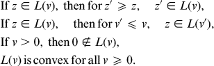 $$\eqalign{ & {\rm If}\,z \in L(v),\,{\rm then}\,{\rm for}\,z' \geqslant z,\quad z' \in L(v), \cr & {\rm If}\,z \in L(v),\quad {\rm then}\,{\rm for}\,v' \leqslant v,\quad z \in L(v'), \cr & {\rm If}\,v \gt 0,\,{\rm then}\,0 \notin L(v), \cr & L(v)\,{\rm is}\,{\rm convex}\,{\rm for}\,{\rm all}\,v \geqslant 0.} $$
Strong disposability of characteristics means that value does not decrease for goods with more of at least one characteristic and no less of the other characteristics. Strong disposability of value means that if characteristics z can produce a given value v, then those characteristicsFootnote 1 can also produce less value. The property of no free lunch means that it is impossible to produce positive value out of zero characteristics.
The idea that characteristics create value can be seen as similar to the idea that labor and capital combine to create the gross domestic product (GDP). To move from the set representation of the technology to a functional representation, we use the directional input distance function of Chambers, Chung, and Färe (Reference Chambers, Chung and Färe1996). The directional distance function is a special case of Luenberger's (Reference Luenberger1992, Reference Luenberger1995) shortage function. Let the directional vector used to scale inputs to the input isoquant of L(v) be represented by g=(g 1,…,g N)∈R +N. The directional input (characteristic) distance function takes the form
 $$\vec D_i (v,z;g) = \max \{ \beta :\quad z - \beta g \in L(v)\}. $$
This distance function gives the maximum contraction in inputs or characteristics such that the remaining characteristics (z−βg) can still generate value v. For z∈L(v), we have  $\vec D_i (z,v;g) \geqslant 0$, with
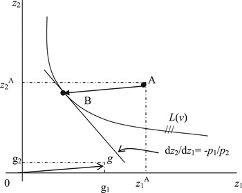
 $\vec D_i (z,v;g) = 0$ indicating that the producer is operating on the input characteristic g-isoquant. Figure 1 illustrates the input correspondence and directional input distance function given a directional vector g=(g 1, g 2). The input correspondence that generates value, v, consists of all characteristics (z 1 and z 2) to the northeast of the curve. A producer (vineyard) has characteristics represented by point A. The directional input distance function for the producer is
 $\vec D_i (v,z;g) = {\textstyle{{AB} \over {0g}}}$.
The Value-Based Input Correspondence, L(v)

The directional input distance function is a complete characterization of the input correspondence in that
 $$\vec D_i (v,z;g) \geqslant 0\quad \Leftrightarrow \quad z \in L(v).$$
In addition, the distance function is monotonic in inputs and value and satisfies the translation property:
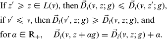 $$\eqalign{ & {\rm If}\,z' \geqslant z \in L(v),{\rm then}\, \vec D_i (v,z;g) \leqslant \vec D_i (v,z';g), \cr & {\rm if}\,v' \leqslant v,{\rm then}\,\vec D_i (v',z;g) \geqslant \vec D_i (v,z;g),{\rm and} \cr & {\rm for}\,\alpha \in {\rm R}_ +, \quad \vec D_i (v,z + \alpha g) = \vec D_i (v,z;g) + \alpha.} $$
Dual to the input distance function is the cost function
 $$C(v,p) = {\min_z} \left\{ {\sum\limits_{n = 1}^n {\,p_n z_n} :\quad z \in L(v)} \right\} ={\min_z} \left\{ {\sum\limits_{n = 1}^N {\,p_n z_n} :\quad \vec D_i (v,z;g) \geqslant 0} \right\}.$$
Following Färe and Primont (Reference Färe and Primont1995) and assuming that p is the shadow (support) price vector for the characteristics, z, the duality between the cost function and the directional input distance function can be summarized as
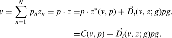 $$\eqalign{v = \sum\limits_{n = 1}^N {\,p_n z_n} = p \cdot z = & p \cdot z^* (v,p) + \vec D_i (v,z;g)pg. \cr = & C(v,p) + \vec D_i (v,z;g)pg.} $$
In words, Equation (7) says that actual costs equal the sum of minimum costs, C(v, p), plus the extra cost of the firm not producing on the input isoquant for value v.
Let the gradient vector of the distance function with respect to z be represented by  $\nabla _z \vec D_i (v,z;g) = \left( {{\textstyle{{\partial \vec D_i (v,z;g)} \over {\partial z_1}}},..., {\textstyle{{\partial \vec D_i (v,z;g)} \over {\partial z_N}}}} \right)$. Then, differentiating Equation (7) with respect to the characteristics yields the price vector
 $$\eqalign{\,p = (\,p_1,..., p_N ) = & \nabla _z \vec D_i (v,z;g)pg \cr = & \left( {\displaystyle{{\partial \vec D_i (v,z;g)} \over {\partial z_1}},..., \displaystyle{{\partial \vec D_i (v,z;g)} \over {\partial z_N}}} \right) \times \sum\limits_{n = 1}^N {\,p_n g_n}.} $$
Multiplying Equation (8) by vector z yields
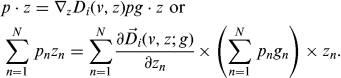 $$\eqalign{ & p \cdot z = \nabla _z D_i (v,z)pg \cdot z \ {\rm or} \cr & {\rm} \sum\limits_{n = 1}^N {\,p_n z_n = \sum\limits_{n = 1}^N {\displaystyle{{\partial \vec D_i (v,z;g)} \over {\partial z_n}} \times \left( {\sum\limits_{n = 1}^N {\,p_n g_n}} \right) \times z_n}}.} $$
Solving Equation (9) for pg yields
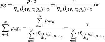 $$\eqalign{ & pg = \displaystyle{{\,p \cdot z} \over {\nabla _z \vec D_i (v,z;g_z ) \cdot z}} = \displaystyle{v \over {\nabla _z \vec D_i (v,z;g_z ) \cdot z}}\,{\rm or} \cr & \sum\limits_{n = 1}^N {\,p_n g_n = \displaystyle{{\sum\limits_{n = 1}^N {\,p_n z_n}} \over {\sum\limits_{n = 1}^N {{\textstyle{{\partial \vec D_i (v,z;g)} \over {\partial z_n}}} \times z_n}}}} = \displaystyle{v \over {\sum\limits_{n = 1}^N {{\textstyle{{\partial \vec D_i (v,z;g)} \over {\partial z_n}}} \times z_n}}}} $$
Then, substituting Equation (10) into Equation (8) yields the hedonic price vector
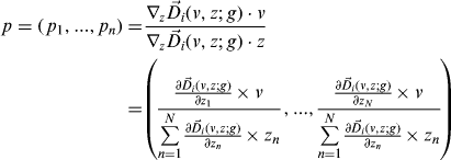 $$\eqalign{\,p = (\,p_1,..., p_n ) = & \displaystyle{{\nabla _z \vec D_i (v,z;g) \cdot v} \over {\nabla _z \vec D_i (v,z;g) \cdot z}} \cr = & \left( {\displaystyle{{{\textstyle{{\partial \vec D_i (v,z;g)} \over {\partial z_1}}} \times v} \over {\sum\limits_{n = 1}^N {{\textstyle{{\partial \vec D_i (v,z;g)} \over {\partial z_n}}} \times z_n}}},..., \displaystyle{{{\textstyle{{\partial \vec D_i (v,z;g)} \over {\partial z_N}}} \times v} \over {\sum\limits_{n = 1}^N {{\textstyle{{\partial \vec D_i (v,z;g)} \over {\partial z_n}}} \times z_n}}}} \right)} $$
Thus, the price of each characteristic can be estimated given the directional input (characteristic) distance function and value using Equation (11). The methodology developed above is an analog to the hedonic price model of Färe, Grosskopf, Sheng, and Sickles (Reference Färe, Grosskopf, Sheng and Sickles2012), who apply Shephard's (Reference Shephard1953) input distance function rather than the directional input distance function. In parameterizing input distance functions different functional forms apply. The directional input distance function is modeled by the quadratic and the Shephard input distance function is modeled by the translog. See Färe, Martins-Filho, and Vardanyan (Reference Färe, Martins-Filho and Vardanyan2010) for a discussion. Since we have zeros for certain inputs in our data, we use the quadratic directional input distance function. In addition, directional input distance functions are capable of modeling cases where some inputs are fixed, such as when regulations require minimum amounts of some inputs be used.
III. The Quadratic Directional Distance Function and Estimation Method
The translog functional form has been widely used to estimate Shephard input or output distance functions. The translog form serves as a second-order approximation to the unknown distance function, and its parameters can be restricted to satisfy the homogeneity property. However, when some firms use zero amounts of some inputs, the logarithmic transformation of the zero input is undefined, with researchers often adding an arbitrarily small positive value to the offending observation. For an example of this use, see Paul, Johnston, and Frengley (Reference Paul, Johnston and Frengley2000). Chambers (Reference Chambers, Färe, Grosskopf and Russell1998) suggests a quadratic form for the directional input distance function. The quadratic form serves as a second-order approximation to the unknown distance function and allows the researcher to impose the translation property on the parameters. Moreover, the quadratic specification allows the possibility of zero inputs, unlike the translog form. Since the data we employ on Oregon vineyards have some vineyards using zero amounts of some inputs, we price vineyard characteristics using the directional distance function estimated from a quadratic form.
We choose a directional vector equal to g=(1, 1,…,1) for all firms in our sample in order to avoid having to parameterize the directional vector, g, into our estimating equation. We assume there are k=1,…,K firms. The quadratic directional input distance function takes the form:
 $$\vec D_i (v_k, z_k ;1) = \beta _0 + \sum\limits_{n = 1}^N {\beta _n z_{nk}} + \displaystyle{1 \over 2}\sum\limits_{n = 1}^N {\sum\limits_{\,j = 1}^N {\beta _{nj} z_{nk} z_{\,jk}}} + \alpha _1 v_k + \displaystyle{1 \over 2}\alpha _2 v_k^2 + \sum\limits_{n = 1}^N {\delta _n z_{nk} v_k}. $$
Symmetry of the second order terms implies that β nj=β jn, n≠j. The distance function also satisfies the translation property in characteristics that yields restrictions on the quadratic form of  $\mathop \sum \nolimits_{n = 1}^N \beta _n = 1,\quad \mathop \sum \nolimits_{\,j = 1}^N \beta _{nj} = 0,\quad n = 1,...,N,\,{\rm and}\,\mathop \sum \nolimits_{n = 1}^N \delta _n = 0.$ To estimate Equation (12), we employ the deterministic method of Aigner and Chu (Reference Aigner and Chu1968). The deterministic method has been used to estimate distance functions and recover shadow prices by English et al. (Reference English, Grosskopf, Hayes and Yaisawarng1993), Färe et al. (Reference Färe, Grosskopf and Weber2001), and Färe, Grosskopf, Noh, and Weber (Reference Färe, Grosskopf, Noh and Weber2005). The deterministic method chooses the parameters β 0, β n, βnj, α 1, α 2, and δ nm so as to minimize the sum of the distances from each firm's observed inputs to the characteristic isoquant for each firm's value. The specific problem we estimate is
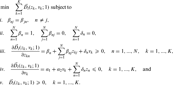 $$\eqalign{ & \min \quad \sum\limits_{k = 1}^K {\vec D_i (z_k, v_k ;1)} \ {\rm subject\,to} \cr & i.\quad \beta _{nj} = \beta _{\,jn}, \quad n \ne j, \cr & ii.\quad \sum\limits_{n = 1}^N {\beta _n = 1,\quad \sum\limits_{\,j = 1}^N {\beta _{nj} = 0,\quad \sum\limits_{n = 1}^N {\delta _n = 0}}}, \cr & iii.\quad \displaystyle{{\partial \vec D_i (z_k, v_k ;1)} \over {\partial z_{kn}}} = \beta _n + \sum\limits_{\,j = 1}^N {\beta _{nj} z_{kj} + \delta _n v_k} \geqslant 0,\quad n = 1,...,N,\quad k = 1,...,K, \cr & iv.\quad \displaystyle{{\partial \vec D_i (z_k, v_k ;1)} \over {\partial v_k}} = \alpha _1 + \alpha _2 v_k + \sum\limits_{n = 1}^N {\delta _n z_n} \leqslant 0,\quad k = 1,...,K,\quad {\rm and} \cr & v.\quad \vec D_i (z_k, v_k ;1) \geqslant 0,\quad k = 1,...,K.} $$
The symmetry and translation restrictions are given by Equations (13i) and (13ii). The distance function is also positively monotonic in characteristics and negatively monotonic in value and these restrictions are given by Equations (13iii) and (13iv). That is, given value (v) an increase in any characteristic (z) will not increase efficiency, and, similarly, given characteristics (z) an increase in value (v) will not decrease inefficiency. Finally, Equation (13v) requires that the observation of characteristics and value for each of the K firms be feasible.
IV. Data and Estimates
To illustrate our method, we price the characteristics of 96 vineyards in Oregon's Willamette Valley that sold between November 1995 and June 2007. Numerous characteristics of the vineyard were recorded. The quality of the acres sold is classified into six segments and ranges from very high quality to low quality. Two other characteristics are the elevation of the acreage and the slope of the acreage. Elevation has nine categories corresponding to acreage with an elevation of less than 240 feet above sea level (the lowest elevation) to the highest elevation corresponding to acreage with an elevation of 500 feet or more above sea level. Slope is classified into six categories ranging from the number of acres with a slope between 0 to 4 degrees up to more than 12 degrees. Furthermore, the aspect of the acreage corresponding to whether it faces west, northwest, north, and so on is available for sixteen different aspect ranges of 22.5 degrees each. Some of the vineyards sold had a dwelling, and the square footage of the dwelling is available. Other vineyards had a barn or winery, and the square footage of these structures is also available. For vineyards with a winery, the cooperage in gallons is available. Soil type is classified into eight different categories corresponding to where the vineyard is located. The American Viticultural Areas (AVA) group the vineyard belongs to is also known and categorized into five different sub-AVAs. Cross, Plantinga, and Stavins (Reference Cross, Plantinga and Stavins2011a, Reference Cross, Plantinga and Stavins2011b) examine vineyard sales prices as a function of the sub-AVA designation, holding other characteristics such as slope and elevation constant. The price premium is highest in the Dundee sub-AVA, followed by Yamhill sub-AVA, Chelahem sub-AVA, Eola Hills sub-AVA, and McMinnville sub-AVA.
The wealth of information on the characteristics of each vineyard is both a blessing and a curse, since only 96 vineyards are available to estimate the quadratic distance function. For instance, if one were to include ten characteristics in the distance function, there would be 74 parameters to estimate once the restrictions corresponding to symmetry and the translation property were imposed. In addition, the characteristics overlap and would result in some double counting. For instance, a hypothetical vineyard might comprise 60 acres, with 30 acres deemed high quality, 20 acres medium-high quality and 10 acres medium quality. Regarding elevation, 15 acres of the hypothetical vineyard are less than 250 feet above sea level and 45 acres are 250 to 300 feet above sea level. Regarding slope for our hypothetical vineyard, 35 acres have a slope of 2 to 4 degrees and 25 acres have a slope of 4 to 6 degrees. Furthermore, 10 acres face southeast and 50 acres face south. However, we do not know the number of high-quality acres with a slope between 2 and 4 degrees that have a southern exposure and an elevation of less than 250 feet. Thus, if each of the characteristics mentioned above is included in the distance function, there is some inevitable degree of double counting.
Faced with these difficulties, we choose a small subset of the characteristics to estimate the distance function and estimate hedonic prices. We focus on the total acreage that is sold. The total acreage is divided into four categories: acres not in the vineyard (z 1), high-quality vineyard acres (z 2), medium-quality vineyard acres (z 3), and low-quality vineyard acres (z 4). Since some, but not all of the properties sold included a dwelling, or a barn, or a winery, we subtract the appraised value of these assets from the sales price to obtain our valuation (v) of the acreage. The valuation of the acreage is deflated by the monthly Consumer Price Index (1982–84=100). In his book Wine Wars, wine economist Mike Veseth (Reference Veseth2011) chronicles the various changes that have occurred in the global wine market. These changes include the opening of new markets in places like China, the relaxation of trade restrictions, changes in packaging ranging from screwtop bottles to cardboard box containers, and the growth in sales of low-price wine such as “Two Buck Chuck.” Such changes have increased competition between producers but also increased demand. To account for these kinds of changes we include a time trend variable, t, ranging from 1 to 14 in the quadratic distance function. We also include indicator variables for the AVA area where the vineyard is located. There are five AVA areas: Chehalem (CH), Dundee (DU), Eola Hills (EA), McMinnville (M), and Yamhill (Y). To avoid an exact linear dependence among the five AVAs, we drop the Yamhill AVA variable in the estimation. The AVA coefficients are reported as ϕ ava, ava=1,…,4. The time trend (γ) and AVA designation will shift the intercept (β 0) for each vineyard.
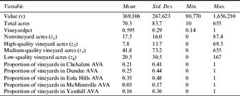
Descriptive statistics are found in Table 1. The 96 vineyards ranged in value from $80,770 to $1,656,210 with an average of $369,106 in 1982–84 constant dollars net of the appraised value of any dwelling, barn, or winery located on the property. The average are was 70.3 acres and ranged from 10 to 655 acres, with an average of 59.5% under cultivation. The average property had 17.5 nonvineyard acres (z 1) , 7.8 high-quality vineyard acres (z 2), 41.8 medium-quality vineyard acres (z 3), and 20.5 low-quality vineyard acres (z 4). Of the 96 vineyards, 21% were located in the Chehalem AVA, 25% in the Dundee AVA, 35% in the Eola Hills AVA, 3% in the McMinnville AVA, and 16% in the Yamhill AVA.
Descriptive Statistics

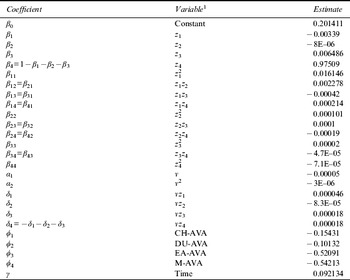
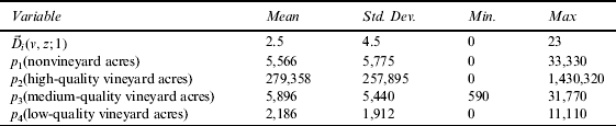
Parameter estimates of the quadratic distance function are reported in Table 2, and estimates of efficiency are reported in Table 3. Fifteen vineyards produced on the efficient frontier with  $\vec D_i (v,z;1) = 0$. The mean value of the directional distance function,
 $\overline {\vec D_i (v,z;1)} = 2.5$, indicates that on average, a vineyard could generate the same level of value using 2.5 fewer acres of each type. The time trend coefficient, γ=0.092, indicates that, with each passing year, the Willamette Valley vineyards can generate the same level of value with approximately 0.092 fewer acres of each of the four types. Relative to vineyards in Yamhill AVA, vineyards in the AVAs of Chelahem (CH), Dundee (D), Eola Hills (EA), and McMinnville (M) are more inefficient. That is, these vineyards could generate the same level of value using fewer inputs than a vineyard in the Yamhill AVA. In contrast, Cross, Plantinga, and Stavins (Reference Cross, Plantinga and Stavins2011a, Reference Cross, Plantinga and Stavins2011b) found an ascending price premium for vineyards in the McMinnville, Eola Hills, Chelahem, Yamhill, and Dundee sub-AVAs. One possible reason for the different results arises from differences in method. We used a deterministic approach and disaggregated total acres into nonvineyard acres and the quantities of acres in the vineyard that were of high, medium, and low quality, whereas Cross, Plantinga, and Stavins used a regression approach and included all vineyard acres as an explanatory variable and then used the shares of acreage with the best and medium soil qualities as additional explanatory variables.
Parameter Estimates of Quadratic Directional Distance Function

1. v=value of vineyard, z 1=nonvineyard acres, z 2=high-quality vineyard acres, z 3=medium-quality vineyard acres, z 4=low-quality vineyard acres, CH=Chelaham AVA, DU=Dundee AVA, EA=Eola Hills AVA, and M=McMinnville AVA.
Estimates of Efficiency and Hedonic Prices
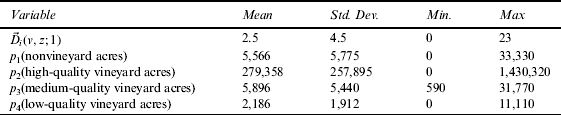
Note: Prices are deflated relative to a base year of 1982–1984.
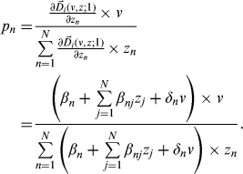
For the quadratic distance function given in Equation (12) the hedonic prices are calculated from Equation (11) as
 $$\eqalign{\,p_n = & \displaystyle{{{\textstyle{{\partial \vec D_i (v,z;1)} \over {\partial z_n}}} \times v} \over {\sum\limits_{n = 1}^N {{\textstyle{{\partial \vec D_i (v,z;1)} \over {\partial z_n}}} \times z_n}}} \cr = & \displaystyle{{\left( {\beta _n + \sum\limits_{\,j = 1}^N {\beta _{nj} z_j + \delta _n} v} \right) \times v} \over {\sum\limits_{n = 1}^N {\left( {\beta _n + \sum\limits_{\,j = 1}^N {\beta _{nj} z_j + \delta _n} v} \right) \times z_n}}}.} $$
We use Equation (14) to calculate the hedonic prices for vineyards that had positive quantities of the characteristics. Each vineyard has different characteristics, z, and value, v, resulting in different hedonic prices for each characteristic. Table 3 reports the means and standard deviations for the hedonic prices for each of the four characteristics for the 96 vineyards. The standard deviations should not be interpreted as standard errors since our estimation method using Equation (13) is deterministic, not stochastic. Instead, the standard deviation of the hedonic price of each characteristic is just a descriptive statistic measuring dispersion. An additional nonvineyard acre is priced at $5,566, a high-quality vineyard acre is priced at $279,358, a medium-quality vineyard acre is priced at $5,896, and a low-quality vineyard acre is priced at $2,186. We further investigate the very high average price of a high-quality vineyard acre. Sixty of the 96 vineyards had zero high-quality acres in their vineyard. For the 60 vineyards without any high-quality acres, the hedonic price of the first acre averaged $403,447. The 36 vineyards with positive high quality acres averaged 7.5 high-quality acres, ranging from a mere half an acre to 27 acres. The average hedonic price per high-quality acre for those 36 vineyards equaled $83,817, ranging from $22,680 to $305,650. Referring again to Figure 1, suppose that high-quality acres are represented by z 2 on the y-axis. Then, an explanation of the relatively high average price per high-quality acre is that almost two-thirds of the vineyards in our sample have no high-quality acres and the directional distance function is projecting them to a relatively flat portion of the input characteristic isoquant, resulting in a very high hedonic price.
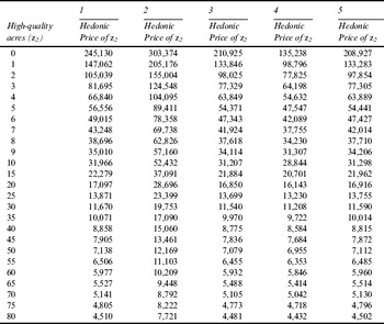
We use the parameter estimates found in Table 2 and the hedonic price equation in Equation (14) to simulate hedonic prices for high-quality vineyard acres, holding the other three input characteristics constant. We consider a hypothetical vineyard with z 1, z 3, z 4, and v equal to the average for those variables given in Table 1, and we allow the number of high-quality vineyard acres (z 2) to range from 0 to 80. The hedonic prices of the high-quality acres for the hypothetical vineyard are reported in Table 4 in column 1. The hedonic price falls rapidly from $147,062 for the first acre to $105,039 for second acre, to $31,966 for the tenth acre, and $4510 for the eightieth acre. The hedonic prices of high quality acres are dependent on the quantities of the other three characteristics and value. We increase each characteristic and value by one standard deviation, holding the other variables constant and report the new set of hedonic prices for high-quality acres in columns 2 to 5 of Table 4. Increasing value (v) by one standard deviation (v=$636,729) and holding z 1, z 3, and z 4 constant at their mean increases the hedonic prices of high-quality acres (column 2). Increasing nonvineyard acres (z 1) by one standard deviation (z 2=33.5), holding v, z 3 and z 4 constant at their mean, lowers the hedonic price of high-quality acres (column 3). Increasing medium-quality acres (z 3) by one standard deviation (z 3=115), holding v, z 1 and z 4 constant, lowers the hedonic price of high-quality acres (column 4). Finally, increasing low-quality acres (z 4) by one standard deviation (z 4=51), holding z 1, z 3, and v at their means, lowers the hedonic price of high-quality acres (column 5).
Simulation of Hedonic Prices of High-Quality Vineyard Acres for a Hypothetical Vineyard

Note: z 1=nonvineyard acres, z 3=medium-quality vineyard acre, z 4=low-quality vineyard acre, and v=vineyard value.
1. z 1=17.5, z 3=41.8, z 4=20.5, and v=$369,106.
2. z 1=17.5, z 3=41.8, z 4=20.5, and v=$636,623.
3. z 1=33.5, z 3=41.8, z 4=20.5, and v=$369106.
4. z 1=17.5, z 3=115, z 4=20.5, and v=$369106.
5. z 1=17.5, z 3=41.8, z 4=51, and v=$369,106.
Our simulation illustrates the usefulness of our approach in calculating hedonic prices. In general, the hedonic price of a characteristic should depend on the amount of the characteristic along with the amounts of other characteristics and value. Models that assign a single hedonic price to a characteristic fail to account for the possibility that characteristics can substitute for one another. Furthermore, our method accounts for the possibility that when value changes, the hedonic prices might change by more or less than that change in value. For instance, the increase in value from $369,106 to $636,729 corresponds to a 72.5% increase, but for a vineyard with only 1 high-quality acre the hedonic price increased by only 23.8%, while it increased by 71% for a vineyard with 80 high-quality acres (see columns 1 and 2 of Table 4).
V. Conclusions
In this paper, we proposed a method of estimating the hedonic prices of characteristics that is theoretically grounded in production theory and accounts for firm inefficiency. Our method exploits the duality between the directional input distance function and the cost function. Unlike shadow pricing models, which require knowledge of the price of at least one input and the marginal rate of substitution between inputs to recover the support price of an unpriced input, our hedonic method recovers the hedonic prices of all unpriced input characteristics, given a differentiable directional distance function and the value (cost) of the bundle of characteristics. We used our method to estimate hedonic prices for four characteristics of 96 vineyards in the Willamette Valley of Oregon that sold between November 1995 and June 2007. The characteristics include the number of acres of high, medium, and low quality in the vineyard as well as the number of nonvineyard acres that are included in the sold parcel. Information on other characteristics such as slope, elevation, and number of acres facing south, southwest, west, and so on are available, but the small number of parcels sold relative to the number of parameters that would have to be estimated preclude us from including these other characteristics. An anonymous referee suggested that principal components analysis might be one way to address this problem, and we leave that suggestion for future work.