1 Introduction
Slender engineering structures are frequently arranged in groups, for example, high-rise buildings, chimney stacks, tube bundles in heat exchangers, chemical-reaction towers, screens, turning vanes in ducts, bridge piers, electronic components on boards and offshore platforms, etc. Naturally, the physics of the flow around closely spaced structures is complicated, involving shear-layer separation/reattachment, quasi-periodic vortices, mutual interactions, separation bubbles, vortex impingement, structural vibration and noise. It is, therefore, very important in both fundamental and practical applications to investigate the detailed physics of the flow around multiple closely spaced structures. A circular or a square cylinder is generally chosen as an investigation model because of their relative simplicity and their frequent occurrence in engineering (Alam, Zhou & Wang Reference Alam, Zhou and Wang2011). While a square prism characterized by a fixed flow separation point, is a representative model of the bluff bodies with sharp corners (e.g. flat plates, square prisms and triangular cylinders), a circular cylinder, characterized by an oscillating separation point, represents bluff bodies with continuous curvature (e.g. circular and elliptical cylinders). The fluid dynamics of the two representative models is, therefore, substantially distinct from each other. Furthermore, a side-by-side arrangement is one of the simplest and most common configurations of multiple slender structures. During the last three decades, there have been extensive investigations on the flow around two circular cylinders in side-by-side arrangements (e.g. Kumada et al. Reference Kumada, Hiwada, Ito and Mabuchi1984; Le Gal et al. Reference Le Gal, Peschard, Chauve and Takeda1996; Alam, Moriya & Sakamoto Reference Alam, Moriya and Sakamoto2003; Alam & Zhou Reference Alam and Zhou2007). However, the flow around multiple square prisms in side-by-side arrangement has received much less attention compared with that around circular cylinders.
For two side-by-side square prisms with
 $L/W=1.02{-}6.00$
(where
 $L$
is the centre-to-centre spacing between the prisms, and
 $W$
is the prism width), Alam et al. (Reference Alam, Zhou and Wang2011), at
 $Re=4.7\times 10^{4}$
, performed systematic measurements of the flow field, Strouhal number and time-mean and fluctuating forces. Four distinct flow regimes, namely (i) single-body regime
 $(1<L/W<1.3)$
, (ii) two-frequency regime
 $(1.3<L/W<2.2)$
, (iii) transition regime
 $(2.2<L/W<3.0)$
and (iv) coupled vortex street regime
 $(L/W>3.0)$
were identified. In addition, shear-layer interaction, gap-flow deflection and changeover, flow entrainment, recirculation bubble, vortex interaction and vortex formation length for each regime were studied in detail and connected to the characteristics of the time-averaged and fluctuating fluid forces. Qualitatively similar observations, based on flow visualization experiments, were made at a smaller
 $Re=300$
by Alam & Zhou (Reference Alam and Zhou2013). Using a two-component laser Doppler velocimeter, Kolar, Lyn & Rodi (Reference Kolar, Lyn and Rodi1997) at
 $Re=2.31\times 10^{4}$
measured the turbulence characteristics in the near wake of two side-by-side prisms at only
 $L/W=3.0$
in the coupled vortex street regime. Agrawal, Djenidi & Antonia (Reference Agrawal, Djenidi and Antonia2006) investigated the laminar wake
 $(Re=73)$
of two prisms at
 $L/W=1.7$
and 3.5, which correspond to the flip-flop and synchronized regimes, respectively, using the lattice Boltzmann method (LBM). They found that the difference between the two regimes could be interpreted in terms of the interaction of the jet formed between the prisms with the adjoining wakes. The degree of the interaction depends on
 $L/W$
.
Investigations on more than two square prisms in side-by-side arrangements are very scarce. Kumar, Sharma & Agrawal (Reference Kumar, Sharma and Agrawal2008) simulated the flow around a row of nine square prisms arranged side-by-side at
 $Re=80$
for
 $L/W=1.3{-}13.0$
, using LBM. Based on vorticity field and drag coefficient signals, they identified three flow regimes, namely synchronized flow, quasi-periodic flow and chaotic flow. No significant interaction between the wakes is observed for
 $L/W>7.0$
. Furthermore, a secondary frequency (resulting from an interaction between prisms) and its implications on the resulting flow are documented. Sewatkar, Sharma & Agrawal (Reference Sewatkar, Sharma and Agrawal2009) investigated the characteristics of the flow across nine square prisms at
 $Re=30{-}140$
for
 $L/W=2.0{-}5.0$
. The critical
 $Re$
for the onset of vortex shedding increases with an increase in
 $L/W$
, and
 $Re$
has a strong effect on the flow, especially at
 $L/W=4.0{-}5.0$
. In addition, the wake interaction is strongly influenced by the jets in the gap region, and the nature of the jets alters with
 $L/W$
and
 $Re$
. Chatterjee, Biswas & Amiroudine (Reference Chatterjee, Biswas and Amiroudine2010) investigated the flow around a row of five square prisms at
 $Re=150$
, with
 $L/W=2.2$
, 3.0, 4.0 and 5.0, using the finite volume method. Three flow regimes are revealed: flip-flopping flow, in-phase and antiphase synchronized flow and non-synchronized flow. They supposed that these flows are a consequence of the interaction between the vortex shedding (primary) and the prism interaction (secondary) frequencies. The flow is dominated by the primary frequency at a higher
 $L/W$
, and the secondary frequency plays an important role in the chaotic flow at a smaller
 $L/W$
. Inoue & Suzuki (Reference Inoue and Suzuki2007) investigated the sound generated by three square prisms placed in a side-by-side arrangement in a uniform flow at low Mach numbers by direct solution of the two-dimensional unsteady compressible Navier–Stokes equations. However, they focused on the effect of
 $L/W$
on sound generation mechanism, not the flow characteristics.
Two side-by-side prisms involving one gap flow is the simplest model to investigate the interaction between the gap and free-stream side flows. On the other hand, three side-by-side prisms involving two gap flows is the simplest and most basic configuration to investigate the interaction between gap and free-stream side flows, as well as that between two gap flows. When
 $L/W$
is large enough (say
 $L/W=3.5$
), coupled-vortex shedding flow was observed for two side-by-side prisms (Alam et al.
Reference Alam, Zhou and Wang2011; Alam, Bai & Zhou Reference Alam, Bai and Zhou2016), and a quasi-periodic flow was identified for a row of an infinite number of prisms (Kumar et al.
Reference Kumar, Sharma and Agrawal2008). In both cases, each prism is accompanied by a single vortex street, with an identical shedding frequency. The initial condition of a prism is the same as that of the other/another. For example, either prism in the two-cylinder case undergoes one gap flow on one side and one free-stream flow on the other side, and a prism in a row of infinite prisms experiences gap flows on either side. The flow around three prisms becomes more complex, incorporating both, with the middle prism experiencing gap flows on either side and an outer prism experiencing a gap flow on one side and a free-stream side flow on the other side. An investigation of three side-by-side prisms can thus bridge the gap between the flows around the two and an infinite number of prisms.
The flow physics around three side-by-side prisms is inconspicuous and cannot be predicted from that around two prisms while an investigation on three prisms can provide us with a better understanding of fundamental aspects of the complicated flow. A number of questions associated with three prisms may emerge. How do the two gap flows interact with each other and with the free-stream side shear layers? How do they influence the wake? How would the flow be classified? The origin of the secondary frequency also deserves attention. Kumar et al. (Reference Kumar, Sharma and Agrawal2008) proposed that the secondary frequency results from a relatively narrow wake behind one of the prisms and a relatively wide wake behind the adjoining prisms, with an interchange between the narrow and wide wakes over time. However, the origin of the secondary frequency is not well understood. In the present study, we focus on the detailed physics of the flow around three side-by-side square prisms. Numerical simulations are performed at
 $Re=150$
for
 $L/W=1.1{-}9.0$
, covering all possible flow regimes. Vorticity fields, shedding frequencies and time series of the aerodynamic force on the three prisms are analysed to explicitly delineate the resultant flow structures. Furthermore, the origin of the secondary frequency and its effect on the lift forces on the prisms are discussed in detail.
2 Computational details
2.1 Governing equations and numerical method
The dimensionless two-dimensional Navier–Stokes and continuity equations governing the flow of a Newtonian fluid can be written in vector form as
 $$\begin{eqnarray}\left.\begin{array}{@{}c@{}}\displaystyle \frac{\unicode[STIX]{x2202}\boldsymbol{u}^{\ast }}{\unicode[STIX]{x2202}t^{\ast }}+\boldsymbol{u}^{\ast }\boldsymbol{\cdot }\unicode[STIX]{x1D735}\boldsymbol{u}^{\ast }=-\unicode[STIX]{x1D735}p^{\ast }+\frac{1}{Re}\unicode[STIX]{x1D6FB}^{2}\boldsymbol{u}^{\ast },\\ \displaystyle \unicode[STIX]{x1D735}\boldsymbol{\cdot }\boldsymbol{u}^{\ast }=0,\end{array}\right\}\end{eqnarray}$$
where
 $\boldsymbol{u}^{\ast }$
is the dimensionless flow velocity vector in the Cartesian coordinate system
 $(x,y)$
with its two velocity components
 $u^{\ast }\;(=u/U_{\infty })$
and
 $v^{\ast }\;(=v/U_{\infty })$
,
 $t^{\ast }\;(=U_{\infty }t/W)$
is the dimensionless time,
 $p^{\ast }\;(=p/\unicode[STIX]{x1D70C}U_{\infty }^{2})$
is the dimensionless static pressure,
 $Re\;(=\unicode[STIX]{x1D70C}U_{\infty }W/\unicode[STIX]{x1D707})$
is the Reynolds number,
 $U_{\infty }$
is the free-stream velocity,
 $W$
is the prism width,
 $\unicode[STIX]{x1D70C}$
is the density of the fluid and
 $\unicode[STIX]{x1D707}$
is the viscosity of fluid. A commercial code, ANSYS-Fluent, was used for the simulations. The finite volume method with a structured quadrangular grid is employed to solve the unsteady two-dimensional incompressible Navier–Stokes equations. The
 $Re$
is kept constant at 150. The gravity force is excluded. The pressure–velocity coupling is handled with the pressure implicit with splitting of operators (PISO) method (Issa Reference Issa1986; Versteeg & Malalasekera Reference Versteeg and Malalasekera2007). Discretization of the convective terms in the equations is accomplished through a second-order accurate upwind differencing scheme. Second-order implicit forward discretization is adopted for the time derivative terms in order to accelerate the convergence process.
The onset vortex street behind a single prism materializes at
 $Re>48$
(e.g. Yoon, Yang & Choi Reference Yoon, Yang and Choi2010). Three-dimensional instability occurs at
 $Re>200$
(Park & Yang Reference Park and Yang2016). Results at a lower
 $Re$
can provide a clear picture of the wake, including shear-layer development, vortex formation and interaction, phase lag between vortex sheddings, etc. Two-dimensional simulations at
 $Re<200$
have thus been adopted in many studies (e.g. Kumar et al.
Reference Kumar, Sharma and Agrawal2008,
 $Re=80$
; Sewatkar, Sharma & Agrawal Reference Sewatkar, Sharma and Agrawal2011,
 $Re=80$
and 160; Sewatkar et al.
Reference Sewatkar, Patel, Sharma and Agrawal2012,
 $40\leqslant Re\leqslant 160$
; Mizushima & Hatsuda Reference Mizushima and Hatsuda2014,
 $40\leqslant Re\leqslant 80$
). The
 $Re=150$
is presently chosen to ensure clear vortex streets. Furthermore, this
 $Re$
facilitates a direct validation of the present results with those in the literature (e.g. Sohankar, Norberg & Davidson Reference Sohankar, Norberg and Davidson1999; Saha, Biswas & Muralidhar Reference Saha, Biswas and Muralidhar2003; Sharma & Eswaran Reference Sharma and Eswaran2004; Kumar et al.
Reference Kumar, Sharma and Agrawal2008). Although a high
 $Re$
is commonly found in many engineering applications (Sumner, Price & Paidoussis Reference Sumner, Price and Paidoussis2000) where the flow is three-dimensional, the wake at both higher and lower
 $Re$
is characterized by Kármán vortex streets. The similarity of the near-wake flow structure for three prisms at
 $L/W=2.5$
between a high and a low
 $Re$
(
 $=4100$
and 150) will be discussed in § 3. The results at a lower
 $Re$
are useful to understand the flow physics at a high
 $Re$
but cannot be directly extrapolated to a high
 $Re$
flow.
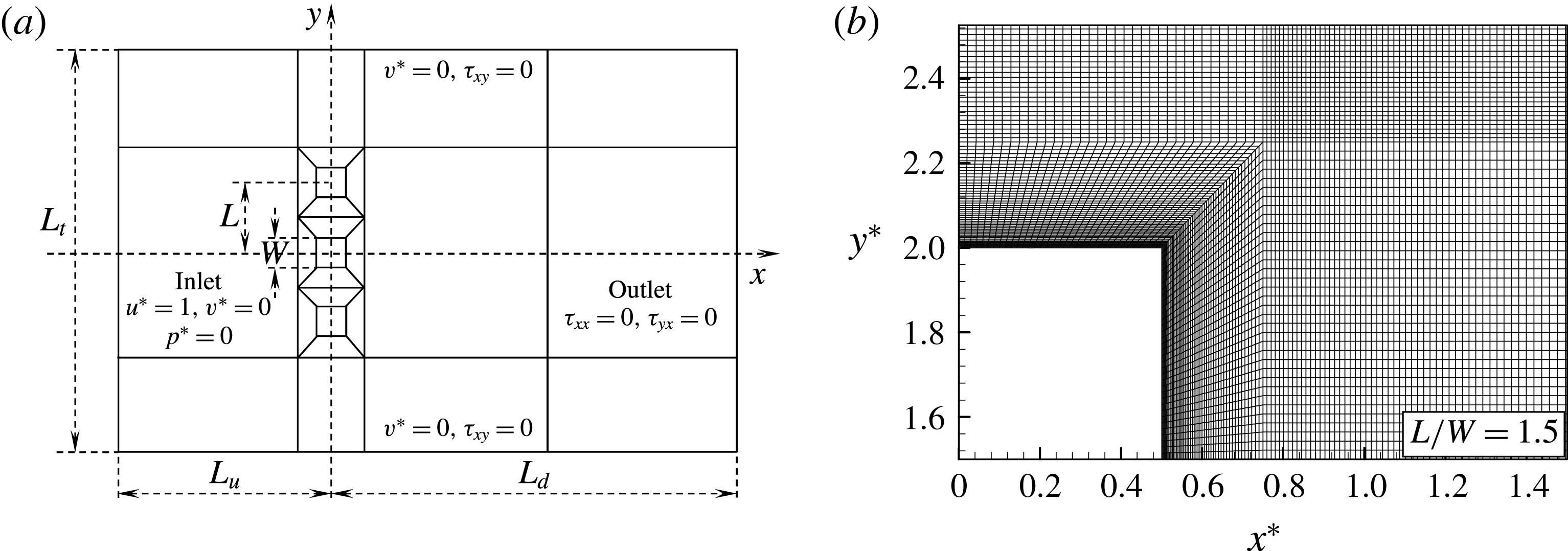
(a) Sketch of the computational domain and boundary conditions, and (b) structured quadrangular grid distribution around a quadrant of a prism.
 $\unicode[STIX]{x1D70F}_{xx}=2\unicode[STIX]{x1D707}(\unicode[STIX]{x2202}u^{\ast }/\unicode[STIX]{x2202}x^{\ast }),\unicode[STIX]{x1D70F}_{xy}=\unicode[STIX]{x1D70F}_{yx}=\unicode[STIX]{x1D707}(\unicode[STIX]{x2202}v^{\ast }/\unicode[STIX]{x2202}x^{\ast }+\unicode[STIX]{x2202}u^{\ast }/\unicode[STIX]{x2202}y^{\ast })$
,
 $x^{\ast }=x/W$
,
 $y^{\ast }=y/W$
.

2.2 Boundary and initial conditions
Figure 1 shows a schematic diagram of the computational domain, boundary conditions, along with the structured quadrangular grid distribution around a quadrant of a prism. As shown in figure 1(a), three square prisms, each of width
 $W$
, are subjected to a uniform flow of velocity
 $U_{\infty }$
. A Cartesian coordinate system is employed such that the origin is at the centre of the middle prism, with the
 $x$
and
 $y$
axes along the streamwise and lateral directions, respectively. The length of the computational domain is
 $L_{x}=L_{u}+L_{d}$
, where
 $L_{u}$
is the upstream length and
 $L_{d}$
is the downstream length from the coordinate origin. The lateral computational boundaries are each
 $L_{t}/2$
away from the middle prism centre. The boundary conditions are summarized as follows. At the inlet boundary, a uniform velocity profile
 $(u^{\ast }=1,v^{\ast }=0)$
is imposed, while the stress vectors are set to zero at the outlet boundary
 $(\unicode[STIX]{x1D70F}_{xx}=2\unicode[STIX]{x1D707}(\unicode[STIX]{x2202}u^{\ast }/\unicode[STIX]{x2202}x^{\ast })=0,\unicode[STIX]{x1D70F}_{yx}=2\unicode[STIX]{x1D707}(\unicode[STIX]{x2202}v^{\ast }/\unicode[STIX]{x2202}x^{\ast }+\unicode[STIX]{x2202}u^{\ast }/\unicode[STIX]{x2202}y^{\ast })=0)$
(Prasanth & Mittal Reference Prasanth and Mittal2008). On the upper and lower lateral boundaries, the component of the velocity normal to and the component of the stress vector along the boundaries are prescribed a zero value (
 $v^{\ast }=0,\unicode[STIX]{x1D70F}_{xy}=\unicode[STIX]{x1D707}(\unicode[STIX]{x2202}v^{\ast }/\unicode[STIX]{x2202}x^{\ast }+\unicode[STIX]{x2202}u^{\ast }/\unicode[STIX]{x2202}y^{\ast })=0$
; symmetry boundary condition) (Prasanth & Mittal Reference Prasanth and Mittal2008; Tong et al.
Reference Tong, Cheng, Zhao and An2015). No-slip boundary conditions
 $(u^{\ast }=v^{\ast }=0)$
are deployed on the surfaces of the square prisms. Furthermore, in the computational domain, the initial flow (at
 $t^{\ast }=0$
) is given as
 $u^{\ast }=1,v^{\ast }=0$
and
 $p^{\ast }=0$
.
2.3 Validation of method and convergence of results
The effect of mesh resolution and locations of the transverse and streamwise computational boundaries on the flow around a single prism is investigated systematically before conducting the extensive simulations. Note that a similar mesh distribution to that used for the single prism is adopted for the three square prisms (figure 1
a). The first level of the grid spacing near the prism wall is set to
 $0.0033W$
for an adequate resolution of the boundary layer. The grid spacing is then increased with an expansion rate of 1.029 in the normal direction (figure 1
b).
2.3.1 Mesh resolution and validation
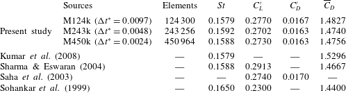
Three different meshes (M124k, M243k and M450k) are utilized to investigate the flow around a single prism. Details of the meshes and integral output (e.g. Strouhal number
 $St$
, time-averaged drag
 $\overline{C}_{D}$
, root mean square (r.m.s.) lift
 $C_{L}^{\prime }$
and drag
 $C_{D}^{\prime }$
coefficients) are presented in table 1. In the present study, the drag (
 $C_{D}$
) and lift (
 $C_{L}$
) coefficients, along with Strouhal number (
 $St$
), are calculated as
 $$\begin{eqnarray}C_{D}=\frac{2F_{x}}{\unicode[STIX]{x1D70C}U_{\infty }^{2}W},\quad C_{L}=\frac{2F_{y}}{\unicode[STIX]{x1D70C}U_{\infty }^{2}W}\quad \text{and}\quad St=\frac{f_{s}W}{U_{\infty }},\end{eqnarray}$$
where
 $F_{x}$
and
 $F_{y}$
are the drag and lift forces, respectively, comprising both pressure and friction forces on a unit length of the prism, and
 $f_{s}$
is the vortex shedding frequency obtained from the power spectrum analysis results of the lift signal. The computational domain size was identical for the three meshes with
 $L_{u}/W=13.5$
,
 $L_{d}/W=29.5$
and blockage ratio
 $=5.26\,\%$
. Note that the maximum Courant numbers were smaller than 1.0 for the meshes M124k
 $(\unicode[STIX]{x0394}t^{\ast }=0.0097)$
, M243k
 $(\unicode[STIX]{x0394}t^{\ast }=0.0048)$
and M450k
 $(\unicode[STIX]{x0394}t^{\ast }=0.0024)$
. The three meshes provide similar output (table 1), with the largest deviation at 2.45 % for
 $C_{L}^{\prime }$
. This establishes the adequacy of mesh M124k for computing the flow past a single isolated prism. Table 1 also compares the results with those from the literature for a single isolated prism at
 $Re=150$
. Overall, the integral parameters (
 $St$
,
 $C_{L}^{\prime }$
,
 $C_{D}^{\prime }$
and
 $\overline{C}_{D}$
) display good agreement with those in the literature.
2.3.2 Effect of the lateral and streamwise locations of the computational boundaries
Blockage ratio effect. Computations are carried out at blockage ratios of 7.69 %, 5.26 % and 3.70 %, and the obtained results are presented in table 2. Note that the upstream and downstream boundary locations are kept fixed (
 $L_{u}/W=13.5$
and
 $L_{d}/W=29.5$
), along with the identical mesh distribution around the prism. It is obvious that
 $St$
,
 $\overline{C}_{D}$
and
 $C_{L}^{\prime }$
all decay with a decrease in the blockage ratio from 7.69 % to 3.7 % (table 2). West & Apelt (Reference West and Apelt1982) concluded that linear corrections can be applied to wind tunnel tests to account for the blockage ratio less than 6 %. Presently, the decrease is small
 $({<}1.2\,\%)$
between the blockage ratios of 5.26 % and 3.7 %. Therefore, the blockage ratio 5.26 % can be acceptable, considering the cost of computing resources.
Effect of mesh resolution on output and comparison of the present results with those from the literature.
 $Re=150$
,
 $L_{u}/W=13.5$
,
 $L_{d}/W=29.5$
and blockage ratio
 $=5.26\,\%$
.

Effect of blockage ratio.
 $Re=150,\unicode[STIX]{x0394}t^{\ast }=0.0097,L_{u}/W=13.5$
,
 $L_{d}/W=29.5$
.

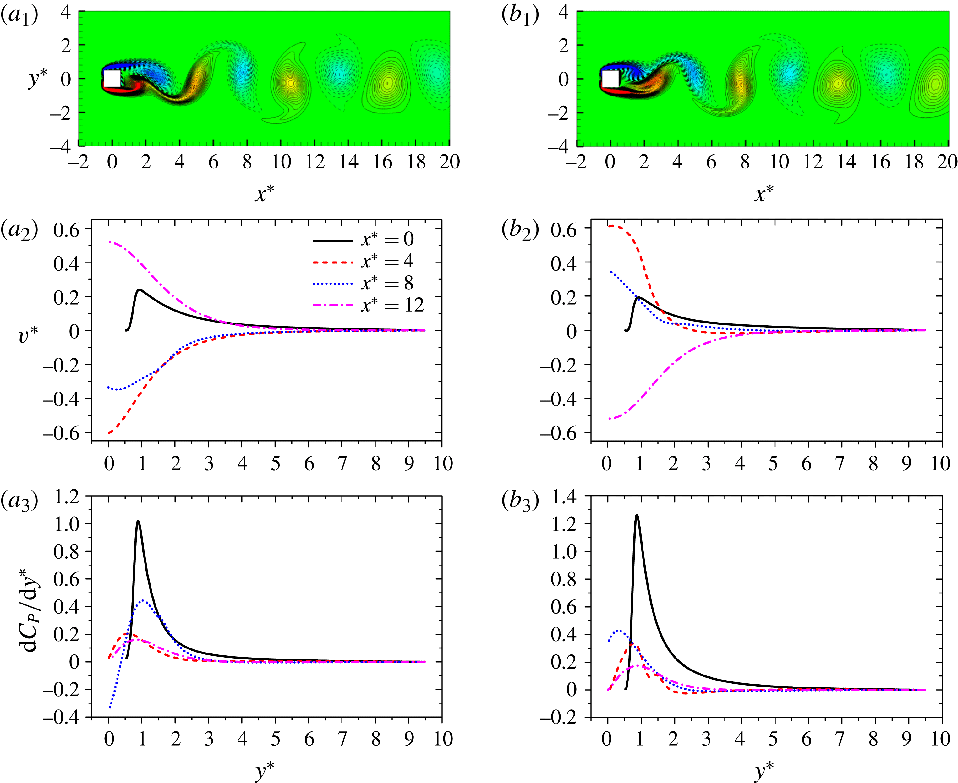
Figure 2(
 $a_{1},\!b_{1}$
) illustrates instantaneous vorticity contours at two representative instants corresponding to the minimum and maximum
 $C_{L}$
, respectively. The distributions of
 $v^{\ast }\;(=v/U_{\infty })$
and pressure coefficient derivative
 $(\text{d}C_{P}/\text{d}y^{\ast })$
along the vertical direction (
 $y^{\ast }=0.0{-}9.5$
) for the two instants are presented in figure 2(
 $a_{2},\!a_{3},\!b_{2},\!b_{3}$
) for
 $x^{\ast }=0.0$
, 4.0, 8.0 and 12.0. While large around the prism,
 $v^{\ast }\approx 0.0$
at
 $y^{\ast }>7.5$
, indicating that the disturbance by the prism is exhausted before reaching the lateral boundary and the assumption about
 $v^{\ast }=0$
at the lateral boundary is valid. As such,
 $\text{d}C_{P}/\text{d}y^{\ast }\approx 0.0$
for
 $y^{\ast }>7.5$
.
(
 $a_{1},\!b_{1}$
) Instantaneous vorticity contours at instants corresponding to minimum and maximum
 $C_{L}$
, respectively. Dependence on
 $y^{\ast }$
of (
 $a_{2},\!b_{2}$
)
 $y$
-component velocity
 $v^{\ast }$
and (
 $a_{3},\!b_{3}$
) pressure coefficient derivative (
 $\text{d}C_{P}/\text{d}y^{\ast }$
) at different
 $x^{\ast }$
.

Effect of the upstream and downstream boundary location. Three simulations are conducted to check the effect of the upstream and downstream boundary locations on the flow around a single isolated prism. The details of computational domain and results obtained with them are listed in table 3. The mesh distribution around the prism as well as the blockage ratio are identical for the three cases. For M124k and M136k,
 $L_{u}/W$
is changed from 13.5 to 25.5, with
 $L_{d}/W=29.5$
fixed. The results from the two sets of computations are in good agreement, with the largest deviation
 $({\approx}1.37\,\%)$
between the two sets of
 $C_{L}^{\prime }$
results. For M124k and M148k,
 $L_{d}/W$
is varied from 29.5 to 51.5, with
 $L_{u}/W=13.5$
fixed. The results are virtually identical while the largest deviation between the two sets of results is for
 $St\;({\approx}0.06\,\%)$
. The computation domain with
 $L_{u}/W=13.5,L_{d}/W=29.5$
, and blockage ratio
 $=5.26\,\%$
, can thus be adopted for the simulation.
Effect of the upstream and downstream boundary locations.
 $Re=150$
,
 $\unicode[STIX]{x0394}t^{\ast }=0.0097$
and blockage ratio
 $=5.26\,\%$
.

2.3.3 Validation of mesh resolution for three prisms
Validations of the mesh resolution and time step for the flow around three prisms are done for the smallest
 $L/W\;(=1.1)$
examined. In the previous sections, the mesh density and time step for the single prism flow are validated at M124 and
 $\unicode[STIX]{x0394}t^{\ast }=0.0097$
, respectively. Given the same mesh density for the three prisms, the total mesh number is M379k for
 $L/W=1.1$
. When the total mesh number is increased to M670k, which corresponds to a 177 % increase in the mesh density,
 $\unicode[STIX]{x0394}t^{\ast }=0.0048$
. The results are presented as cases 1 and 2 in table 4. Note that, the results for the outer prisms (prisms 1 and 3) are identical. The
 $St$
,
 $C_{L}^{\prime }$
,
 $\overline{C}_{L}$
and
 $\overline{C}_{D}$
are thus presented for prisms 1 and 2 only (table 4). It is observed that the largest differences in
 $St$
,
 $C_{L}^{\prime }$
,
 $\overline{C}_{L}$
and
 $\overline{C}_{D}$
between two cases are 1.7 %, 1.2 %, 1.4 % and 0.8 %, respectively. Therefore, the mesh density employed is large enough to resolve the flow field around the three prisms.
Effects of the mesh resolution on the flow around three prisms at
 $L/W=1.1$
.
 $Re=150$
, blockage ratio
 $=5.26\,\%,L_{u}/3W=13.5,L_{d}/3W=29.5$
.

3 Experimental details and results
Particle image velocimetry (PIV) and smoke-wire flow visualization experiments were conducted in a closed-loop low-speed wind tunnel with a test section of length 5.0 m, width 0.8 m and height 1.0 m. The flow velocity in the test section was uniform to 0.1 % (r.m.s.) and the longitudinal turbulence intensity was less than 0.4 %. Three square prisms of width
 $W=15~\text{mm}$
, made of aluminium, were arranged side-by-side with
 $L/W=2.5$
and mounted horizontally across the width of the tunnel, resulting in a blockage ratio of 4.5 %. Experiments were conducted at a free-stream velocity
 $U_{\infty }=4~\text{m}~\text{s}^{-1}$
, corresponding to
 $Re=4100$
.
The flow was seeded by particles, generated from paraffin oil, with a particle size of approximately
 $1.0~\unicode[STIX]{x03BC}\text{m}$
in diameter. A light sheet, approximately 0.8 mm thick, illuminated the flow, produced by two Newwave standard pulse laser sources at 532 nm wavelength, each with a maximum energy output of
 $120~\text{m}\text{J}~\text{pulse}^{-1}$
. Particle images were captured using a charge-coupled device (CCD) camera (Vision Phantom V641, double frames,
 $2560\times 1600$
pixels). An adaptive PIV method with an interrogation window of
 $16\times 16$
pixels was used with 50 % overlap in each direction. A total of 2400 PIV images were captured to calculate time-averaged streamlines. The same PIV system was used for smoke-wire visualization experiments under the same flow conditions. A stainless steel wire of 0.1 mm diameter was installed vertically across the height of the wind tunnel approximately 15 mm upstream of the prisms. The wire was coated with smoke-generator fluid (paraffin oil) which was evaporated by electrically heating the steel wire (DC regulated power supply-70 V).
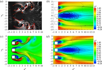
Comparison of experimental (a,b) and simulation (c,d) results for three side-by-side square prisms. (a) Smoke-wire flow visualization result, (b) PIV measured time-averaged streamwise velocity
 $\bar{u}^{\ast }\;(=\bar{u}/U_{\infty })$
field (colour coded) and streamline,
 $Re=4100$
. Simulated (c) instantaneous vorticity field and (d)
 $\bar{u}^{\ast }$
field (colour coded) and streamline,
 $Re=150$
. The arrows in (a) indicate the rolling direction of shear layers and vortices.
 $L/W=2.5$
.

Figure 3 compares the experimental and simulation results at
 $L/W=2.5$
. Although
 $Re=4100$
employed in the experiment is different from that (
 $Re=150$
) in the simulation, the results obtained from the two techniques agree reasonably well, extracting key features. The gap flows are symmetrically biased outward (figure 3
a,c); the recirculation region behind the middle prism is thus larger compared with that behind an outer prism (figure 3
b,d). The streamwise length of the recirculation region behind the middle prism is
 $7.75W$
and
 $8.04W$
in the experimental and simulation results, respectively, slightly elongated in the simulation results. A similar elongation is discernible for the recirculation regions behind the outer prisms. The deviation may arise from the difference between the Reynolds numbers (Zdravkovich Reference Zdravkovich1997).
Dependence of flow regimes on
 $L/W$
:
 $A$
, base-bleed flow
 $(L/W<1.4)$
;
 $B$
, flip-flopping flow
 $(1.4<L/W<2.1)$
;
 $C$
, symmetrically biased beat flow
 $(2.1<L/W<2.6)$
;
 $D$
, non-biased beat flow
 $(2.6<L/W<7.25)$
;
 $E$
, weak interaction flow
 $(7.25<L/W<9.0)$
.

4 Flow structures and forces
Simulations were performed for a total of 22
 $L/W$
between
 $L/W=1.1$
and 9.0. For
 $L/W>9.0$
, the flow behind each of the prisms was virtually identical to that of the single isolated prism. The adjacent wakes interacted with each other in a complicated manner at
 $L/W<7.25$
, resulting in five distinct flow structures. The corresponding
 $L/W$
ranges of the flow structures are given in figure 4:
 $A$
, base-bleed flow
 $(L/W<1.4)$
;
 $B$
, flip-flopping flow
 $(1.4<L/W<2.1)$
;
 $C$
, symmetrically biased beat flow
 $(2.1<L/W<2.6)$
;
 $D$
, non-biased beat flow
 $(2.6<L/W<7.25)$
; and
 $E$
, weak interaction flow
 $(7.25<L/W<9.0)$
. Each flow regime has distinct intrinsic features associated with vortex structures, shear-layer behaviours, gap-flow deflections, shedding frequencies and force characteristics, etc. The border between two consecutive flow modes is identified with the midpoint between two adjacent simulated
 $L/W$
where one flow mode changes to another. For example, the flow structures at
 $L/W=1.3$
and 1.5 are determined to be base-bleed flow (regime
 $A$
) and flip-flopping flow (regime
 $B$
), respectively. The border is then made at
 $L/W=1.4$
. The corresponding uncertainty in determining the critical
 $L/W$
is
 $\pm 0.1,\pm 0.1,\pm 0.1$
and
 $\pm 0.25$
between regimes
 $A$
and
 $B$
,
 $B$
and
 $C$
,
 $C$
and
 $D$
and
 $D$
and
 $E$
, respectively. Next, we will discuss each flow regime based on vorticity structures, time-mean streamwise velocities, lift forces and power spectra of fluctuating lift forces. The time-mean flow field was based on the sample duration of more than 200 predominant vortex shedding cycles. Particularly, for flip-flopping regime, the sample duration was longer at more than 600 cycles.
Contours of instantaneous vorticity and time-averaged streamwise velocity
 $\bar{u}^{\ast }\;(=\bar{u}/U_{\infty })$
at (a,b)
 $L/W=1.1$
and (c,d)
 $L/W=1.2$
. (e) Variation in
 $\bar{u}^{\ast }$
across the wake at
 $x^{\ast }=1.0$
and 5.0.
 $t^{\prime }$
is the time delay measured from the instant (i) that corresponds to a
 $C_{L}$
peak of the prism 1, and
 $\unicode[STIX]{x1D70F}_{1}$
is the shedding period of the same prism. Regime
 $A$
.

4.1 Regime A: base-bleed flow
 $(L/W<1.4)$

The base-bleed flow (regime
 $A$
) prevails at
 $L/W<1.4$
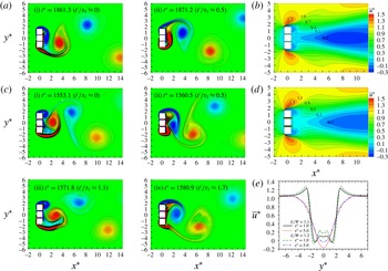
. Figure 5 displays instantaneous vorticity structures at
 $L/W=1.1$
and 1.2, revealing that the vortex shedding essentially occurring from the outer (free-stream) sides of the outer prisms results in a single vortex street. The gap flows between the prisms appear very weak at
 $L/W\leqslant 1.1$
(figure 5
a) and appreciable at
 $1.1<L/W<1.4$
(figure 5
c). As will be discussed later, this difference has a pronounced impact on fluid forces and the shedding frequency. As such, regime
 $A$
may be further subdivided into two: weak base-bleed flow
 $(L/W\leqslant 1.1)$
and strong base-bleed flow
 $(1.1<L/W<1.4)$
. The shedding, appearance, and shape of the vortices in the wake, are more regular at
 $L/W=1.1$
(figure 5
a) than at
 $L/W=1.2$
(figure 5
c). At
 $1.1<L/W<1.4$
, the flows through the two gaps are prone to bias toward the growing vortex near the base (figure 5
c). Indeed, the growing vortex rolling near the base, giving rise to highly negative pressure, attracts the gap flows. When a vortex from the lower side grows rapidly, accumulating vorticity, both gap flows swerve to the lower side (figure 5
c (i, iii)). In the next half-cycle of the vortex shedding, the upper vortex grows and pulls the gap flows toward the upper side (figure 5
c (ii, iv)). As shown above, the gap flows between the prisms appear very weak at
 $L/W=1.1$
and appreciable at
 $L/W=1.2$
. Considerable amounts of opposite sign vorticity, originating from the gap flows, are entrained by the shear layer in the vortex shedding process. This opposite sign vorticity is added to the vorticity cancellation process, enabling a faster pinch off. The shedding frequency is thus larger for
 $L/W=1.2$
than for
 $L/W=1.1$
. Alam et al. (Reference Alam, Zhou and Wang2011) for two side-by-side cylinders at
 $Re=4.7\times 10^{4}$
found perfectly single bluff-body and single bluff-body-like flow for
 $L/W\leqslant 1.02$
and
 $1.02<L/W<1.3$
, respectively.
The contours of time-averaged streamwise velocity
 $\bar{u}^{\ast }(=\bar{u}/U_{\infty })$
at
 $L/W=1.1$
and 1.2 are presented in figure 5(b,d). The
 $\bar{u}^{\ast }$
patterns for
 $L/W=1.1$
and 1.2 are similar, either showing a single large recirculation region
 $(\bar{u}^{\ast }<0)$
in the wake. The recirculation region, however, retreats for
 $L/W=1.2$
due to a larger momentum passing through the gap. In order to highlight the variation in
 $\bar{u}^{\ast }$
across the wake,
 $\bar{u}^{\ast }$
profiles at
 $x^{\ast }=1.0$
and 5.0 are presented in figure 5(e). For
 $L/W=1.1,\bar{u}^{\ast }$
at
 $x^{\ast }=1.0$
is almost constant behind the middle prism
 $(-0.5<y^{\ast }<0.5)$
and forms two valleys at
 $y^{\ast }=\pm 1.32$
and two peaks
 $(\bar{u}^{\ast }>1.0)$
at
 $y^{\ast }=\pm 2.69$
(figure 5
e). While the two peaks represent the shear layers from the free-stream sides of the prisms, the reverse flows due to the vortex sheddings generate the two valleys. At the same
 $x^{\ast }$
, the
 $\bar{u}^{\ast }$
for
 $L/W=1.2$
displays similar behaviour except for two more peaks
 $(\bar{u}^{\ast }<1.0)$
prevailing at
 $y^{\ast }=\pm 0.60$
. The additional peaks correspond to the flows through the gaps. The absence of the corresponding peaks for
 $L/W=1.1$
implies that the flows through the gaps are very weak, as observed in figure 5(a). At
 $x^{\ast }=5.0$
, a single large valley materializes for either
 $L/W$
, suggesting the occurrence of a single vortex street.
Time histories of lift forces on the three prisms and their power spectral density (PSD) functions at
 $L/W=1.1$
(a,b) and
 $L/W=1.2$
(c,d). Regime
 $A$
. The instants marked in the lift histories correspond to the flow structures in figure 5.

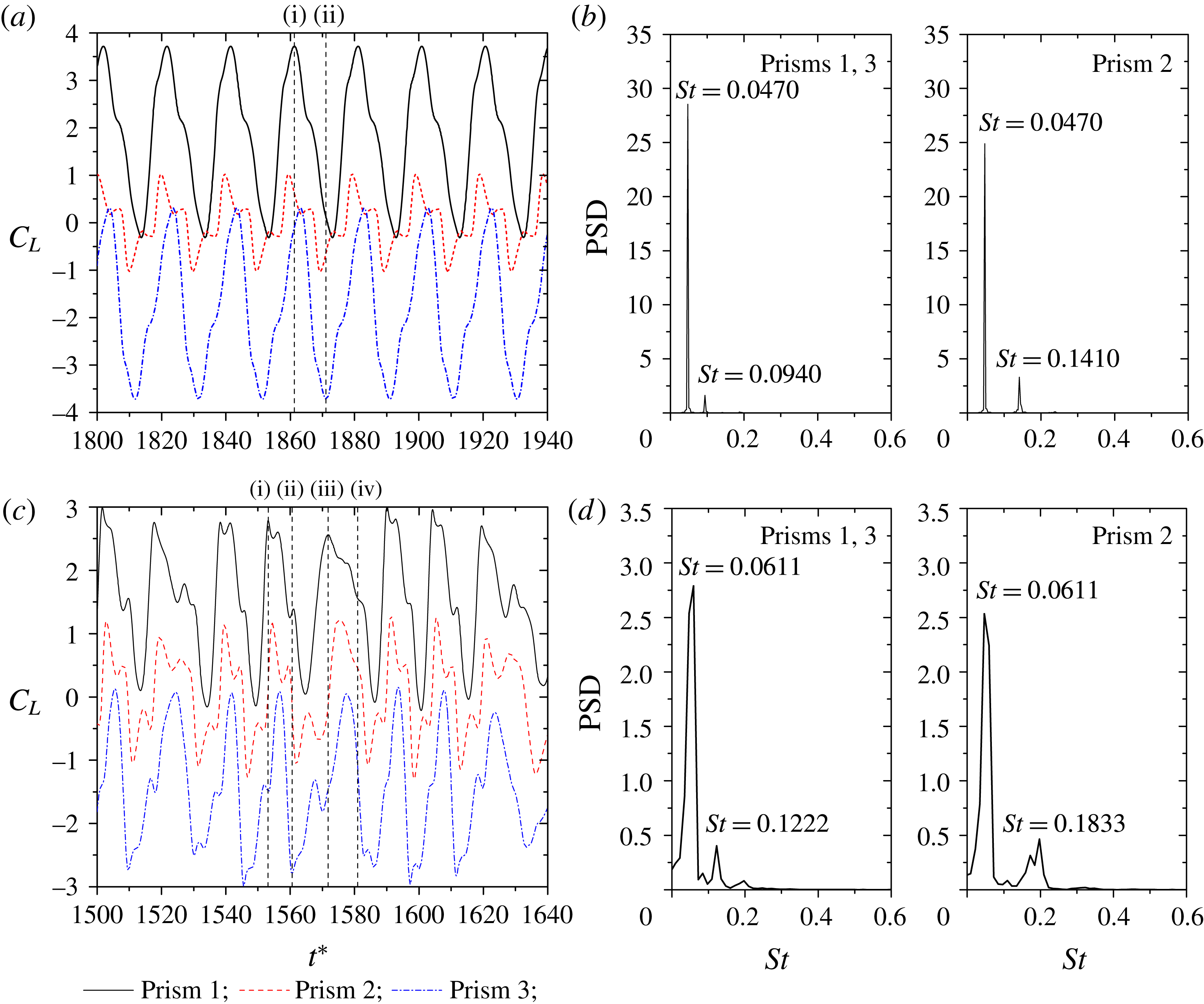
Figure 6 shows time histories of
 $C_{L}$
on the three prisms and their power spectra at
 $L/W=1.1$
and 1.2. Evidently, at
 $L/W=1.1$
, the amplitude of the lift fluctuation is the same for the two outer prisms (prisms 1 and 3) and much larger than that for the middle prism (prism 2). The time-mean lift is positive
 $({\approx}2.22)$
, zero and negative
 $({\approx}\!-\!2.22)$
for the prisms 1, 2 and 3, respectively, i.e. repulsive mean lift for the outer prisms. The gap flows play a significant role at
 $L/W=1.2$
where the lift signals of three prisms are irregular in both amplitude and period (figure 6
c). The irregularity emerges from the fact that the gap flows, constrained by the prism side surfaces, cannot be synchronized with the sheddings from the free-stream sides. The momentum passing through the gaps is dependent on the instantaneous phase lag between the sheddings from a free-stream side and the gaps. When the instantaneous phase lag becomes smaller, the negative pressure behind the prism, due to the vortex formation from the free-stream side, can attract more fluid through the gaps. The momentum passing through the gaps may thus become larger. The phase lag also affects the shedding period and
 $C_{L}$
amplitude. As seen in figure 6(c),
 $C_{L}$
amplitude and shedding period for the prism 1 are larger and shorter, respectively, at instant (i) compared to their counterparts at instant (iii), due to a shorter instantaneous phase lag between prisms 1 and 2 at the former instant than the latter. That is, a smaller phase lag results in a shorter period and a larger amplitude and vice versa. The period in lift signals (figure 6
c) thus repeatedly varies from short to long; see also figure 5
c (i,
 $t^{\ast }=1553.1$
) and (ii,
 $t^{\ast }=1560.5$
) covering approximately one half of the short period and figure 5
c (iii,
 $t^{\ast }=1571.8$
) and (iv,
 $t^{\ast }=1580.9$
) covering approximately one half of the long period. Therefore, the spectral peaks for
 $L/W=1.2$
are less pronounced and broadbanded (figure 6
d), and those for
 $L/W=1.1$
are pronounced and slim (figure 6
b). The
 $St=0.0611$
at
 $L/W=1.2$
(figure 6
d) corresponds to the mean of the short and long periods repeatedly varying from one to the other due to a change in the phase lag discussed above, while
 $St=0.0470$
is connected to the regular shedding frequency at
 $L/W=1.1$
(figure 6
b). There are small peaks at the second and third harmonics for the outer and middle prisms, respectively, resulting from the interaction between the gap flows and vortices from the free-stream sides. For the weak base-bleed flow, considering three prisms as one single entity, the effective
 $St$
based on the total height
 $(2L+W)$
is estimated to be
 $0.1504~(L/W=1.1)$
, slightly less than that of the single prism
 $(St_{0}=0.1579)$
at
 $Re=150$
(table 1) and greater than
 $St_{0}=0.1350$
(Okajima Reference Okajima1982; Sohankar Reference Sohankar2006) at the corresponding effective
 $Re=480\;(=3.2\times 150)$
based on
 $2L+W\;(=3.2W)$
. The difference might be connected to the effective cross-section being modified from square to rectangular. On the other hand, it is much larger, 0.2077 at
 $L/W=1.2$
, indicating the role of the gap flows in the shedding process.
(a) Sequential contours of instantaneous vorticity field displaying vortex shedding from the three prisms. The gap flows biased (i) upward, (ii) outward, (iii) downward and (iv) straight.
 $t^{\prime }$
is the time delay measured from the instant (i) that corresponds to a
 $C_{L}$
peak of the prism 1 and
 $\unicode[STIX]{x1D70F}_{1}$
is the shedding period of the same prism. (b) Contours of time-averaged streamwise velocity
 $\bar{u}^{\ast }\;(=\bar{u}/U_{\infty })$
. (c) Variation in
 $\bar{u}^{\ast }$
across the wake at
 $x^{\ast }=1.0$
and 5.0.
 $L/W=1.7$
(regime
 $B$
).

4.2 Regime B: flip-flopping flow
$(1.4<L/W<2.1)$

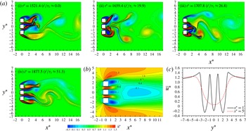
When
 $L/W$
is increased to regime
 $B\;(1.4<L/W<2.1)$
, a greater flow can pass through the gaps and can split the wake into three (figure 7
a). Appreciable vortices from the gaps are shed and merge with the free-stream side vortices. The gap flows can now flip-flop randomly in different fashion, directed upward (figure 7
a (i)), outward (figure 7
a (ii)), downward (figure 7
a (iii)) and straight (figure 7
a (iv)), generating the four different flow structures. However, although the gap flows are biased and flip flopping, a single combined wake dominantly forms behind the three prisms. The nature and
 $L/W$
range of the flip-flopping flow are different from those for two side-by-side cylinders. As observed by Alam et al. (Reference Alam, Zhou and Wang2011) for two side-by-side cylinders in flip-flopping regime, three solutions exist; one is symmetric, where the gap flow is straight, and other two are asymmetric where the gap flow is biased upward or downward. Spontaneous switching, without any perturbation, of the gap flow, was observed with the two asymmetric flows having equal probability. A change in the phase lag between the two vortices from the gap leads to the switch of the gap flow (Alam & Zhou Reference Alam and Zhou2013). As obtained presently, four solutions for the three prisms are possible, the gap flow being straight, symmetrically biased outward or asymmetrically biased upward and downward (figure 7
a). The switch of the flow from one to another was random, again upward and downward biased flows are expected to be of an equal probability.
The
 $\bar{u}^{\ast }$
contours (figure 7
b) illustrate three small recirculation bubbles transmuting to a single one at
 $x^{\ast }>4$
. The
 $\bar{u}^{\ast }$
value at the two peaks caused by the gap flows at
 $x^{\ast }=1.0$
is now greater than 1.0, comparable to that associated with the free-stream side shear layers (figure 7
c), indicating the occurrence of the vortex shedding from the gaps as well as from the free-stream sides. The three wakes correspond to the three valleys, respectively (figure 7
b,c). The middle valley (at
 $y^{\ast }=0$
) is slightly sharper than the other two. The gap-flow peaks, occurring at the gap centrelines, are almost symmetric about their axes. They vanishing at
 $x^{\ast }=5.0$
give rise to a single large valley (figure 7
b,c), which implies that the three wakes merge into one.
Time histories of (a) lift and (b) drag forces on the three prisms: (i)
 $t^{\ast }=1521.4$
, (ii)
 $t^{\ast }=1659.4$
, (iii)
 $t^{\ast }=1707.8$
and (iv)
 $t^{\ast }=1877.5$
marked in the lift and drag histories correspond to the flow structures in figure 7. (c) The power spectral density functions of lift forces of the three prisms,
 $L/W=1.7$
(regime
 $B$
).

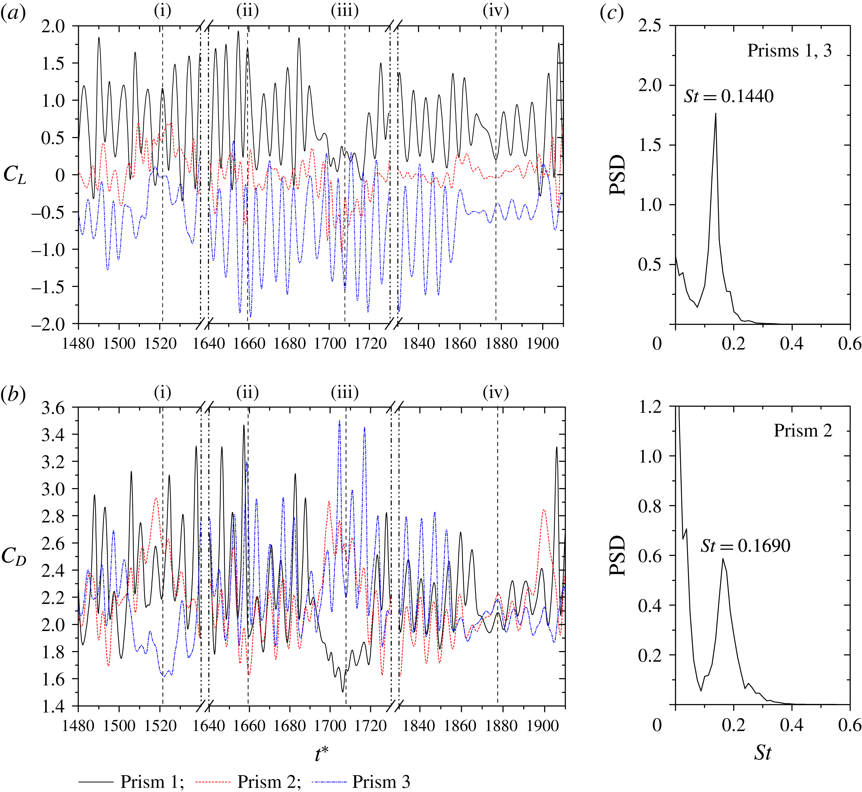
Figure 8 illustrates the time histories of
 $C_{L}$
and
 $C_{D}$
, and the power spectra of
 $C_{L}$
at
 $L/W=1.7$
. The
 $C_{L}$
and
 $C_{D}$
of three prisms are more chaotic than those in regime
 $A$
, owing to the unstable characteristics of the gap flows. The four instantaneous wake structures in figure 7(a) correspond to the instants marked by (i), (ii), (iii) and (iv) in figure 8(a,b), respectively. When the gap flows are biased upward or downward (figure 7
a (i), (iii)), a wide wake accompanies one of the outer prisms, and two narrow wakes complement the other two prisms. A narrow wake having a smaller formation length implies a higher drag and higher fluctuations in lift and drag, regardless of whether it is located behind an outer or the middle prism (figures 7
a, 8). The three wakes are comparable to one another when the gap flows are not biased appreciably (figure 7
a (iv)).
 $C_{L}$
and
 $C_{D}$
characteristics, thus, do not differ between the three prisms (figure 8
a,b, instant iv). The power spectra of
 $C_{L}$
shown in figure 8(c) exemplify that
 $St$
compared to that for the base-bleed flow jumps to 0.1440 (0.1379–0.1501, broadbanded) for both outer prisms and 0.1690 (0.1630–0.1750, broadbanded) for the middle prism. The flip-flopping of the wakes results in the broadbanded
 $St$
. The middle prism
 $St$
is higher than the outer prisms’, indicating that the middle prism undergoes the narrow wake most of the time (figure 7
a (i), (iii)). The difference in Strouhal numbers between the middle and outer prisms may result in a defective vortex shedding in an interval of
 $\unicode[STIX]{x0394}t^{\ast }\approx 1/(0.169{-}0.144)=40$
. Some radical irregularities (e.g. instant iii, prism 1; instant iii, prism 3) in
 $C_{L}$
and
 $C_{D}$
variations, due to defective sheddings, are observed in figure 8(a), but their occurrences are not regular due to the wide band
 $St$
.
Sequential snapshots (instantaneous vorticity field) showing the merging process of vortices when the gap flows are deflected downward.
 $L/W=1.7$
(regime
 $B$
). Dimensionless time
 $t^{\prime }/\unicode[STIX]{x1D70F}_{3}$
is given at the upper left corner, where
 $t^{\prime }$
is the time delay measured from the instant (a) and
 $\unicode[STIX]{x1D70F}_{3}$
is the shedding period of the prism 3 when the gap flows deflect downward.

The important features identified above are (a) a single combined wake forms downstream, (b) the middle prism has the largest
 $St$
, (c) the wide and narrow wakes behind the outer prisms correspond to a smaller and an intermediate
 $St$
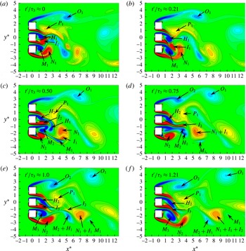
, respectively and (d) a wide band peak prevails in the power spectra. These features can further be elucidated from the interaction of vortices in one period of the vortex shedding. When the gap flows are deflected downward, figure 9 shows typical sequential photographs in one vortex shedding period of the lower prism. It is observed that the flow from each gap has a tendency to shed the two counter-rotating vortices almost simultaneously. As displayed in figure 9(a), the shear layers from the two sides of the lower gap are inclined downward because vortex
 $I_{1}$
leads vortex
 $M_{1}$
. So do those of the upper gap,
 $P_{1}$
leading
 $H_{1}$
(Alam & Zhou Reference Alam and Zhou2013).
 $I_{1}$
and
 $M_{1}$
moving toward the lower free-stream side tend to merge with vortex
 $N_{1}$
(figure 9
b); but
 $N_{1}$
and
 $I_{1}$
, because of the same sign of rotations, merge first forming a larger vortex
 $N_{1}+I_{1}$
and keep
 $M_{1}$
abreast (figure 9
c,d). When the two same-sign vortices (
 $N_{1}$
and
 $I_{1}$
) come closer, they provide opposite-sign velocities at their interface. The opposite-sign velocities bring about the merging process. As the directions of velocities at the interface between
 $M_{1}$
and
 $N_{1}+I_{1}$
are the same, a low pressure occurring at the interface, acting as a tie, keeps
 $M_{1}$
and
 $N_{1}+I_{1}$
abreast (Alam & Zhou Reference Alam and Zhou2013).
 $M_{1}$
, which is smaller, thus orbits around and does not separate from
 $N_{1}+I_{1}$
. Due to a difference in the shedding frequencies from the two sides of the lower gap, new vortex
 $M_{2}$
slightly leads
 $I_{2}$
, causing the gap flow to be almost straight (figure 9
c,d). Again, the clockwise vortices
 $M_{2}$
and
 $H_{1}$
, because of the same sign of their rotations, come closer and merge, forming
 $M_{2}+H_{1}$
(figure 9
d,e).
 $I_{2}$
, having the opposite sign of rotation, cannot merge with
 $M_{2}+H_{1}$
, but they, staying abreast, approach
 $N_{1}+I_{1}$
(figure 9
e).
 $N_{1}+$
 $I_{1}$
and
 $I_{2}$
are again of the same sign of rotation, hence merge easily and form a combined vortex
 $N_{1}+I_{1}+I_{2}$
which couples with
 $M_{2}+H_{1}$
. As
 $M_{2}+H_{1}$
, rotating ahead of
 $N_{1}+I_{1}$
, may have a larger convection velocity, the rotation of
 $N_{1}+I_{1}$
pushes
 $M_{2}+H_{1}$
toward the free-stream side (figure 9
d,e).
 $M_{2}+H_{1}$
thus accelerates, coming in the free-stream side where the flow velocity is generally higher. In the lower side, now six vortices (
 $N_{1}+I_{1}+I_{2}$
,
 $M_{1}$
,
 $M_{2}+H_{1}$
) are combined and coupled (figure 9
f); the clockwise vortices (
 $M_{2}+H_{1}$
,
 $M_{1}$
) vanish rapidly, as the lower side of the combined wake is auspicious only for anticlockwise vortices.
As seen, vortices
 $P_{1}$
and
 $O_{1}$
accumulate anticlockwise vorticity (figure 9
a) respectively from the lower and upper sides of the upper prism for a longer period (smaller shedding frequency). Interestingly, while the clockwise vortices from the free-stream side of the upper prism feature the upper side of the combined wake, the anticlockwise vortices from the lower side of the upper prism and amalgamated anticlockwise vortices characterize the lower side of the combined wake in the downstream. Counting the numbers of vortices shed from the upper and lower prisms (figure 9
a–e), it can be stated that the shedding period is longer and shorter for the upper and middle prisms, respectively, compared to their counterpart in the lower prism. The opposite relationship takes place when the gap flows are deflected upward (figure 7
a (i)).
(a) Contours of instantaneous vorticity field showing vortex shedding from the prisms. The arrows in the figures indicate trajectories of the paired vortices.
 $t^{\prime }$
is the time delay measured from the instant (i) that corresponds to a
 $C_{L}$
peak of the prism 1 and
 $\unicode[STIX]{x1D70F}_{1}$
is the shedding period of the same prism. (b) Schematic of amalgamation and pairing process, showing velocities at the interfaces between the vortices. (c) Contours of time-averaged streamwise velocity
 $\bar{u}^{\ast }\;(=\bar{u}/U_{\infty })$
. (d) Variation in
 $\bar{u}^{\ast }$
across the wake at
 $x^{\ast }=1.0$
and 5.0.
 $L/W=2.5$
(regime
 $C$
).

4.3 Regime C: symmetrically biased beat flow
$(2.1<L/W<2.6)$

Symmetrically biased beat flow occurring at
 $2.1<L/W<2.6$
(regime
 $C$
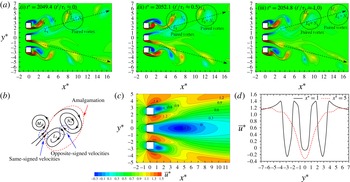
) is characterized by the gap flows being biased/diverged outward symmetrically (figure 10
a); a substantial wide wake thus accompanies the middle prism and a narrow wake complements each outer prism. As illustrated in figure 10(a), the flow structure is very similar to that in figure 7
a (ii), implying that the development of the symmetrically biased flow occurs in regimes
 $B$
–
 $C$
. For symmetrically biased beat flow, the vortex sheddings from the outer prisms are found to be interlocked with a constant phase lag
 $\unicode[STIX]{x1D719}=180^{\circ }$
(antiphase). Note that here interlocked means the interlock between the vortex sheddings from the outer prisms only, as the vortex shedding pattern of the middle prism is different from that of the outer prisms. The two shear layers of the middle prism spawn vortices almost symmetrically, not alternately, in the upper and lower wakes, respectively. Vortex
 $L_{1}$
leading
 $M_{1}$
moves toward the upper wake and meets vortex
 $N_{1}$
from the free-stream side (figure 10
a (i),b). The same-sign vortices
 $L_{1}$
and
 $N_{1}$
integrate and form a larger vortex
 $L_{1}+N_{1}$
which pairs with the opposite-sign vortex
 $M_{1}$
(figure 10
a (ii,iii),b). Therefore, two rows of vortices on the free-stream sides feature the combined wake in the downstream. The phase lag between the two gap vortices (say,
 $L_{1}$
and
 $M_{1}$
) changes periodically, leading to a change in the flow following a beat which will be discussed later.
The
 $\bar{u}^{\ast }$
contours show that the bubble behind the middle prism is very large compared to that behind an outer prism (figure 10
c). The
 $\bar{u}^{\ast }$
profile at
 $x^{\ast }=1.0$
displays three valleys and two gap-flow peaks (figure 10
d). The features of the valleys and peaks are nevertheless different from those in regime
 $B$
. The differences can be outlined as (a) the gap flow peaks are not symmetric about their axes but are skewed inward, (b) the valley associated with the middle prism is blunter and wider in
 $y^{\ast }$
than the other two and (c) the lateral
 $(y^{\ast })$
separation between the two peaks for the gap flows is broader than that for a gap flow and a free-stream side shear layer. All these points explicate that the gap flows are symmetrically biased outward (figure 10
a). The
 $\bar{u}^{\ast }$
distribution at
 $x^{\ast }=5.0$
displays a wide and deep valley around
 $y^{\ast }=0$
, two small peaks at
 $y^{\ast }=\pm 3.45$
and two small valleys at
 $y^{\ast }=\pm 4.30$
. In other words, the two outer valleys and the two peaks associated with the gap flows at
 $x^{\ast }=1.0$
shift outward at
 $x^{\ast }=5.0$
, becoming small.
Time histories of (a) lift and (b) drag forces acting on the prisms: (i)
 $t^{\ast }=2049.4$
, (ii)
 $t^{\ast }=2052.1$
and (iii)
 $t^{\ast }=2054.8$
marked in the lift and drag histories correspond to the flow structures in figure 10. (c) The power spectral density functions of lift forces of the three prisms.
 $L/W=2.5$
(regime
 $C$
).

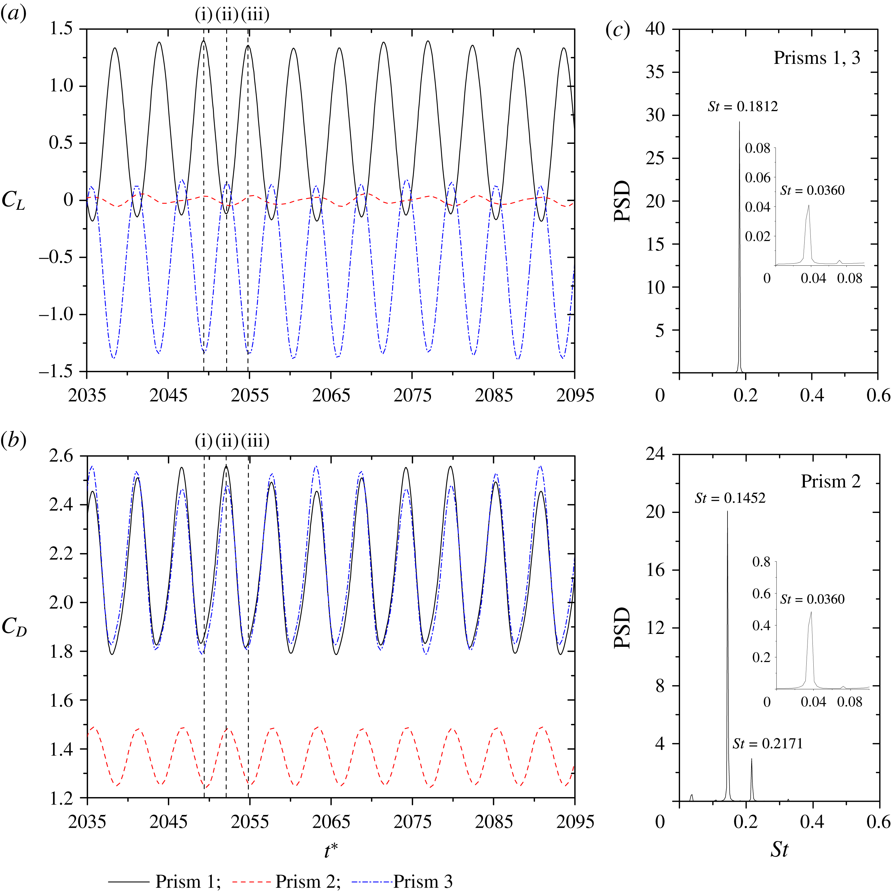
Figure 11(a,b) shows
 $C_{L}$
and
 $C_{D}$
signals of the three prisms at
 $L/W=2.5$
. The lift signals of the outer prisms are sinusoidal and antiphase (figure 11
a), reflecting a constant period. On the other hand, the lift of the middle prism, with a very small amplitude, seems composed of two frequencies, with a short and a long period appearing alternately. The small amplitude suggests an almost symmetric shedding, and the presence of the two frequencies will be discussed later. It is worth mentioning that the
 $C_{L}$
and
 $C_{D}$
amplitudes, particularly for the outer prisms, are not constant, but grow and shrink periodically with time (figure 11
a,b). The power spectra shown in figure 11(c) provide more information on the frequencies. While a dominant
 $St=0.1812$
appears for the outer prisms,
 $St=0.1452$
and 0.2171 are discernible for the middle prism (figure 11
c). The shedding from the middle prism, generating a wide wake, corresponds to
 $St=0.1452$
. The other
 $St\;(=0.2171)$
of the middle prism may be a signature of the interaction between the vortices of
 $St=0.1812$
and 0.1452 as
 $2\times 0.1812{-}0.1452$
. Furthermore, a tiny peak at
 $St=0.0360$
(see the insets) is observed for both middle and outer prisms. Hereafter, this
 $St$
is referred to as the secondary or beat frequency associated with the periodical variation in amplitudes or peaks of lift and drag. As expected, a change in the flow with time following a beat is responsible for the periodical variation in amplitudes or peaks of
 $C_{L}$
and
 $C_{D}$
. The phenomenon of the beat frequency would be also found in the next flow regime. The origin of the beat flow and beat frequency and their effects on the lift will be discussed in § 6 later.
(a) Contours of instantaneous vorticity field showing vortex shedding from the prisms, where the instantaneous phase lag between the vortex sheddings from the middle and outer prisms changes with time but that from the two outer prisms does not.
 $t^{\prime }$
is the time delay measured from the instant (i) that corresponds to a
 $C_{L}$
peak of the prism 1 and
 $\unicode[STIX]{x1D70F}_{1}$
is the shedding period of the same prism. (b) Contours of time-averaged streamwise velocity
 $\bar{u}^{\ast }\;(=\bar{u}/U_{\infty })$
. (c) Variation in
 $\bar{u}^{\ast }$
across the wake at
 $x^{\ast }=1.0$
and 5.0.
 $L/W=3.5$
(regime
 $D$
).

4.4 Regime D: non-biased beat flow
$(2.6<L/W<7.25)$

As
 $L/W$
is large enough (
 $2.6<L/W<7.25$
, regime
 $D$
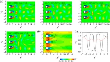
), the gap flows are no longer biased and a single vortex street, qualitatively similar to that behind an isolated prism, persists behind each prism (figure 12
a). Again the vortex sheddings from the outer prisms occurring at the same frequency are coupled with a fixed phase lag
 $\unicode[STIX]{x1D719}$
. Here, it should be noted that
 $\unicode[STIX]{x1D719}$
depends on
 $L/W$
, decaying from
 $160.8^{\circ }$
to
 $0^{\circ }$
between
 $L/W=2.7$
and 3.5, and remains
 ${\approx}0^{\circ }$
at
 $3.5\leqslant L/W\leqslant 4.0$
before increasing gradually to
 $134.8^{\circ }$
at
 $L/W=7.0$
. The vortex shedding frequency of the middle prism is however different to and higher than that of the outer prisms. The instantaneous phase relationship between the vortex sheddings from the middle and outer prisms thus changes periodically from antiphase to in phase (figure 12
a (i–iv)), and vice versa, which has a great impact on the time histories of
 $C_{L}$
of the prisms. The contours of
 $\bar{u}^{\ast }$
and its variation across the wake presented in figure 12(b,c) are thus different from those for regime
 $C$
. There is no appreciable difference in the recirculation bubble size between the middle and an outer prism. At
 $x^{\ast }=1.0$
, the three valleys resemble one other, and the gap flows generate two symmetric plateaus in
 $\bar{u}^{\ast }$
(centred at
 $y^{\ast }=\pm 1.75$
, figure 12
c), instead of the two skewed peaks seen in regime
 $C$
(figure 10
d). The three valleys at
 $x^{\ast }=5.0$
keep their identities separate, and they are almost similar to one another in terms of both shape and minimum
 $\bar{u}^{\ast }$
.
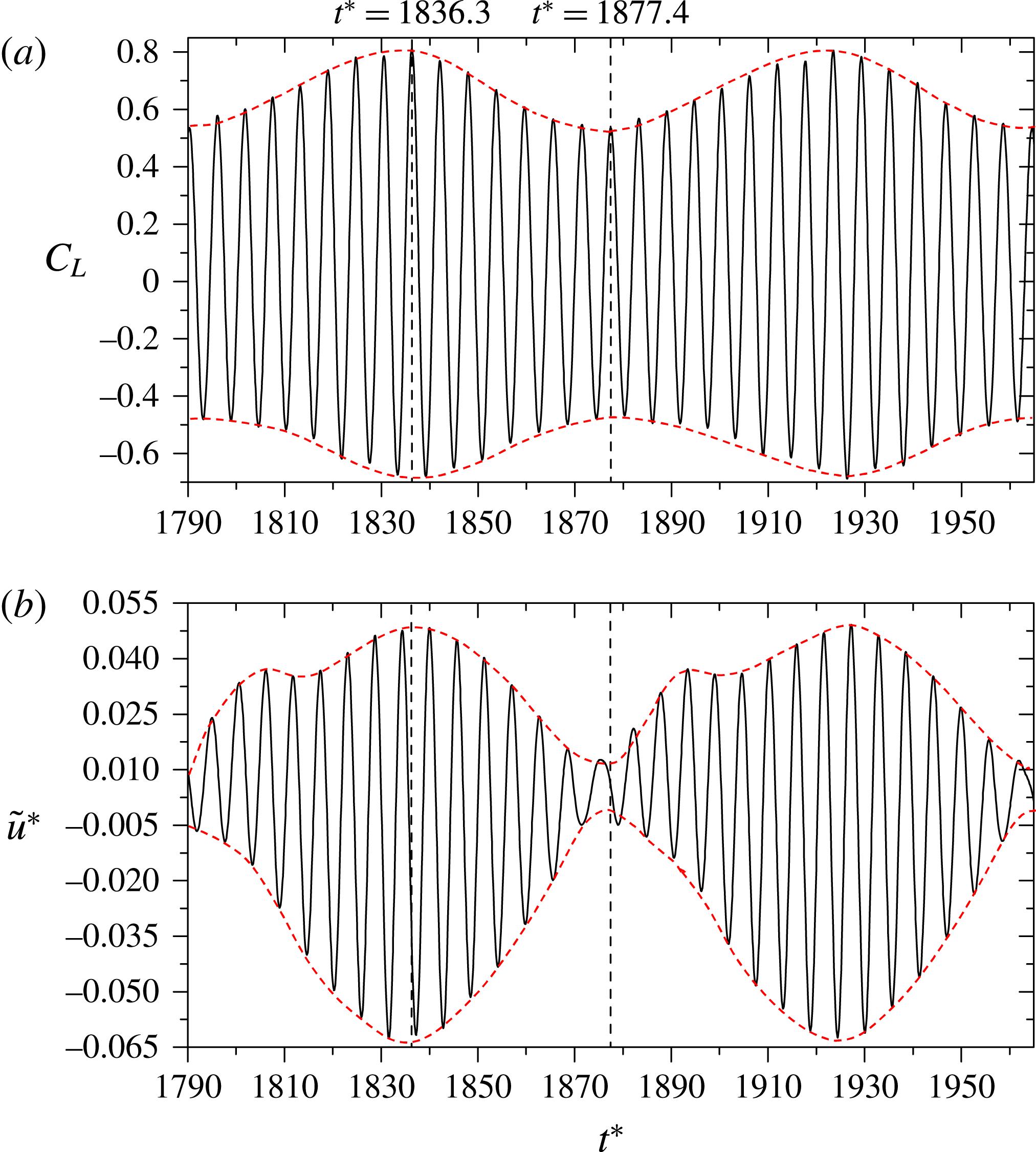
(a) Time histories of lift forces on the three prisms and (b) Instantaneous phase lag between lift fluctuations of the upper and middle prisms: (i)
 $t^{\ast }=1836.3$
, (ii)
 $t^{\ast }=1847.9$
, (iii)
 $t^{\ast }=1859.6$
and (iv)
 $t^{\ast }=1877.4$
correspond to the flow structures given in figure 12. (c) Power spectral density functions of lift forces. Here
 $L/W=3.5$
(regime
 $D$
).

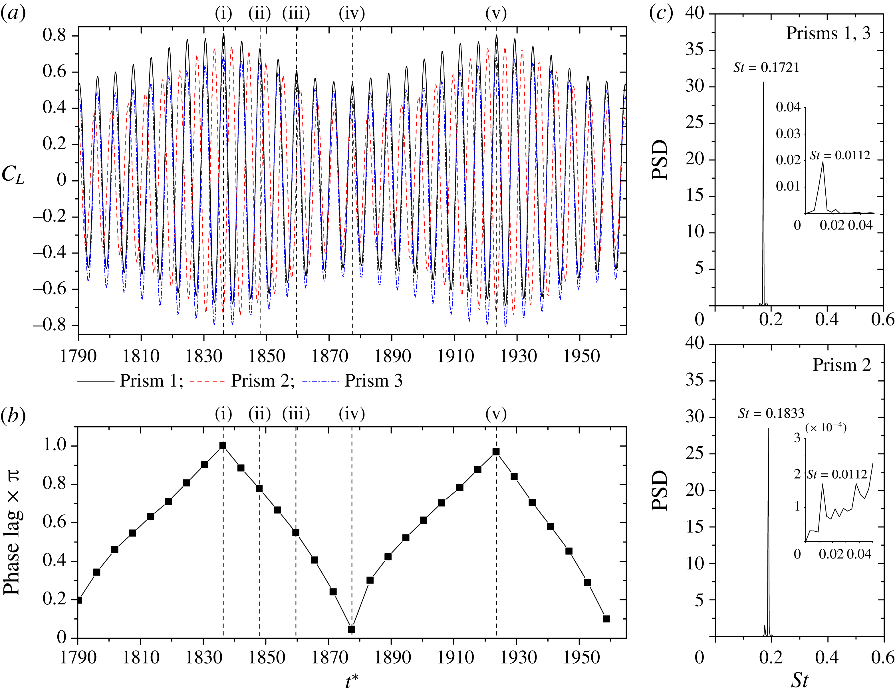
Time histories of
 $C_{L}$
of the three prisms at
 $L/W=3.5$
and their power spectra are shown in panels 13(a) and 13(c), respectively. Each power spectrum features a dominant, very narrowband, peak. The peak corresponds to
 $St=0.1833$
and 0.1721 for the middle and outer prisms, respectively (figure 13
c).
 $St=0.0112$
seen in the insets emerges as the difference between the Strouhal numbers of the middle and outer prisms, associated with the beat frequency. The difference in the Strouhal numbers leads to an obvious beat-like variation in the amplitudes of the
 $C_{L}$
histories (figure 13
a). The vortex sheddings from the outer prisms at
 $L/W=3.5$
are always in phase; see the lift signals in figure 13(a) and shedding patterns in figure 12(a). Note that the flow structures in figure 12
a (i, ii, iii, and iv) are respectively at the instants (i), (ii), (iii) and (iv) marked in the
 $C_{L}$
signals in figure 13(a). Due to the difference in the Strouhal numbers between the middle and outer prisms, the instantaneous sheddings from the middle and outer prisms, depending on the time, can be antiphase (figure 12
a (i)) or in phase (figure 12
a (iv)). Indeed, the antiphase and in-phase sheddings are associated with the maximum and minimum
 $C_{L}$
amplitudes (figure 13
a). That is, the flow transmutes from in phase to antiphase and vice versa following a beat. An interaction between the vortices from the gaps occurs, resulting in an irregularity of vortex arrangement and a decay of vortices particularly behind the middle prism (figure 12
a). The irregularity and decay of vortices with
 $x^{\ast }$
, however, crop up at a smaller
 $x^{\ast }$
for in-phase shedding (figure 12
a (iv)) than the antiphase shedding (figure 12
a (i)), both agree with the corresponding
 $C_{L}$
fluctuations. That is, the beat-like variation in
 $C_{L}$
is connected to the instantaneous phase lag between the sheddings from the middle and outer prisms. The instantaneous phase lag between the middle and outer prisms is thus calculated by the time interval between the adjacent peaks corresponding to the maximum
 $C_{L}$
(associated with the primary frequency) of the middle and one of the outer prisms, normalized by the primary shedding period of the outer prisms (figure 13
b). As seen, the instantaneous phase lag has a periodical change, reaching
 ${\approx}\unicode[STIX]{x03C0}$
at
 $t^{\ast }=1836.3$
,
 ${\approx}0$
at
 $t^{\ast }=1877.4$
, and again
 ${\approx}\unicode[STIX]{x03C0}$
at
 $t^{\ast }=1923.5$
, with a non-dimensional period
 $T^{\ast }=1923.5{-}1836.3=87.2$
and corresponding frequency
 $1/T^{\ast }=0.0114$
that is almost identical to the secondary
 $St=0.0112$
. The information further establishes the relationship between the beat-like variation in amplitudes and phase lag. It will be shown later that an increased
 $L/W$
will correspond to a smaller secondary frequency. The beat-like modulation will thus be weaker and can be ignored at
 $L/W>7.25$
.
(a) Contours of instantaneous vorticity field showing vortex streets. Here
 $t^{\prime }$
is the time delay measured from the instant (i) that corresponds to a minimum
 $C_{L}$
of the prism 1, and
 $\unicode[STIX]{x1D70F}_{1}$
is the shedding period of the same prism. (b) Lift force signals and (c) power spectral density functions of the lift forces,
 $L/W=9.0$
(regime
 $E$
): (i)
 $t^{\ast }=2066.0$
; (ii)
 $t^{\ast }=2218.0$
.

4.5 Regime E: weak interaction flow
$(7.25<L/W<9.0)$

At a large spacing (
 $L/W>7.25$
, regime
 $E$
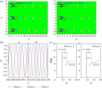
), the interaction between the adjacent wakes is weak. So is the interlocking tendency (constant phase lag) between the sheddings from the outer prisms. Shown in figure 14 are instantaneous vorticity structures and
 $C_{L}$
histories along with their power spectra for
 $L/W=9.0$
. The shedding from each prism resembles that from an isolated prism, and the three vortex streets spaced sufficiently do not interact with one another (figure 14
a). The difference in the Strouhal numbers between the middle and outer prisms is now small, with
 $St=0.1600$
for the middle prism and
 $St=0.1581$
for the outer prisms (figure 14
c). Due to the difference in the Strouhal numbers between the middle and outer prisms, the phase lag between the middle and outer prisms changes continuously, giving an in-phase shedding from the upper two prisms and antiphase from the lower two prisms (figure 14
a (i),b) and an opposite sequence of in-phase and antiphase sheddings (figure 14
a (ii),b). The in-phase and antiphase sheddings, however, do not influence much the lift forces on the prisms because of the large
 $L/W$
and lack of interaction between the streets. The secondary frequency is thus not observed in the lift force signals (figure 14
b) or in the power spectra (figure 14
c).
(a) Variations in Strouhal number (
 $St$
), modified Strouhal number (
 $St_{mod}$
) and wake Strouhal number (
 $St^{\ast }$
) with
 $L/W$
. (b) Variations in time-mean maximum streamwise velocity (
 $\bar{u}_{max}^{\ast }$
) in the shear layers and boundary layer separation velocity
 $(\bar{u}_{b}^{\ast })$
based on base pressure coefficient (
 $C_{pb}$
). Note that
 $\bar{u}_{max}^{\ast }=$
 $\bar{u}_{max}/U_{\infty }$
,
 $\bar{u}_{b}^{\ast }=$
 $\bar{u}_{b}/U_{\infty }=\sqrt{1-C_{pb}}$
.

4.6 Dependence of Strouhal number on
$L/W$
and its connection with the flow classification

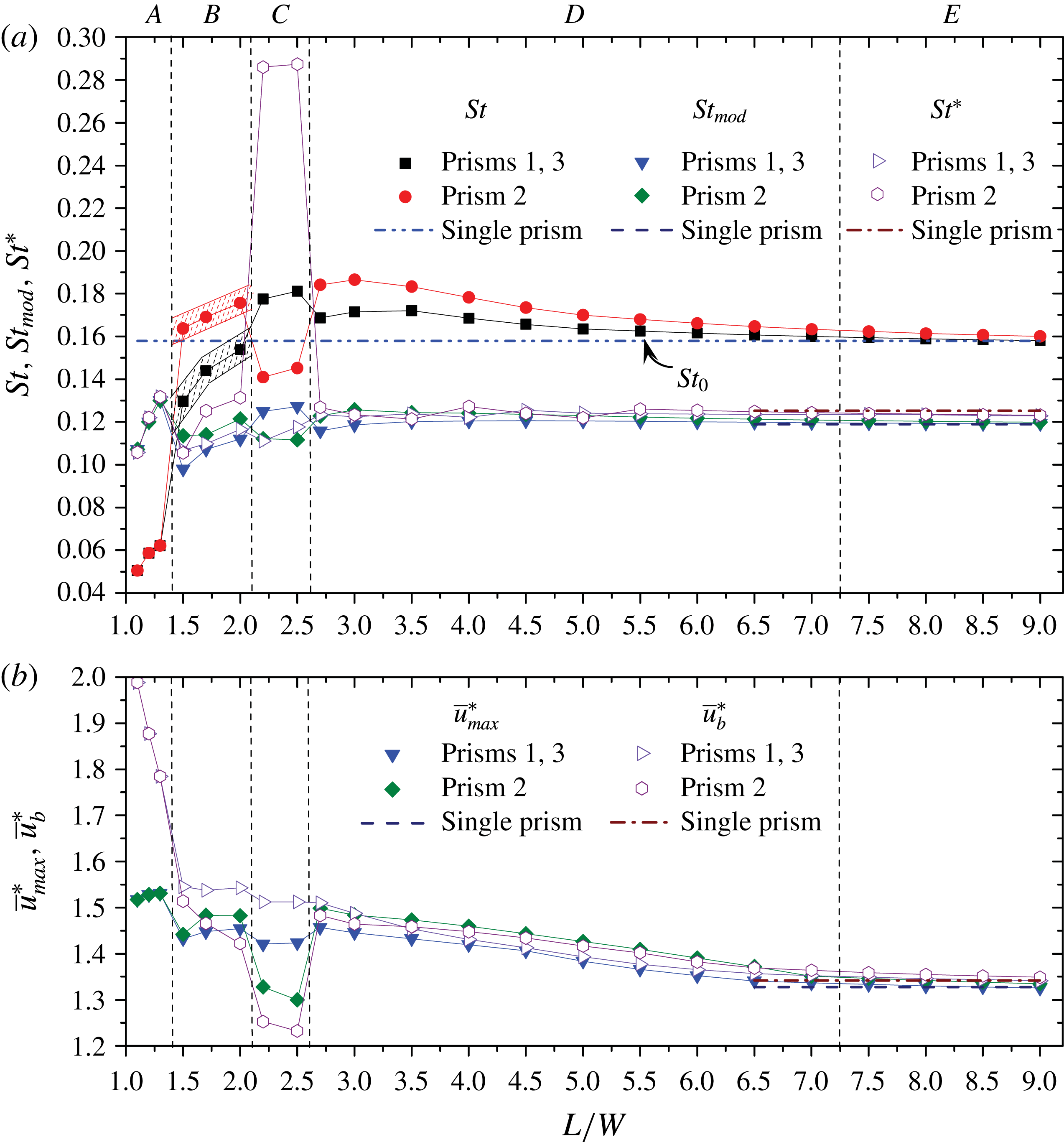
It would be interesting to see how the flow classification is connected to
 $St$
. Figure 15(a) shows variations in
 $St$
with
 $L/W$
. As the two outer prisms have the same
 $St$
regardless of
 $L/W$
,
 $St$
of the two outer prisms is represented by a closed square symbol, and that of the middle prism is denoted by a closed circle. The flow regimes are marked at the top of the figure. The
 $St$
is small and identical for the three prisms at base-bleed flow (regime
 $A$
), associated with a single combined wake behind the prisms. It augments the effect of
 $L/W$
as is influenced by the increased gap flows. At flip-flopping flow (regime
 $B$
),
 $St$
of the middle prism jumps to a higher value as the gap flows now can split the single wake into three. Due to a change in the instantaneous phase lag between the counter-rotating vortices from each gap, the gap-flow deflection also varies accordingly. The
 $St$
thus has a band (see hatched) for both middle and outer prisms. The shedding from the outer prisms is more regular than that from the middle (figures 7, 8), with the latter prism mostly experiencing a narrow wake. The middle prism
 $St$
switches to a smaller value drastically when
 $L/W$
is increased to regime
 $C$
where a wide wake behind the middle prism prevails. Simultaneously, the outer prism
 $St$
keeps escalating. A leap and a drop of
 $St$
occurring for the middle and outer prisms, respectively, separate regime
 $D$
from regime
 $C$
. At regime
 $D$
, the relative difference of the
 $St$
between the middle and outer prisms decays with
 $L/W$
. Decay also occurs for the outer prisms
 $St$
, but at a smaller rate. The difference in the Strouhal numbers between the middle and outer prisms thus tapers off with
 $L/W$
, suggesting that the interaction between the sheddings from the prisms weakens. The difference is small in regime
 $E$
, reflecting a very weak interaction between the sheddings. Besides, the magnitude of
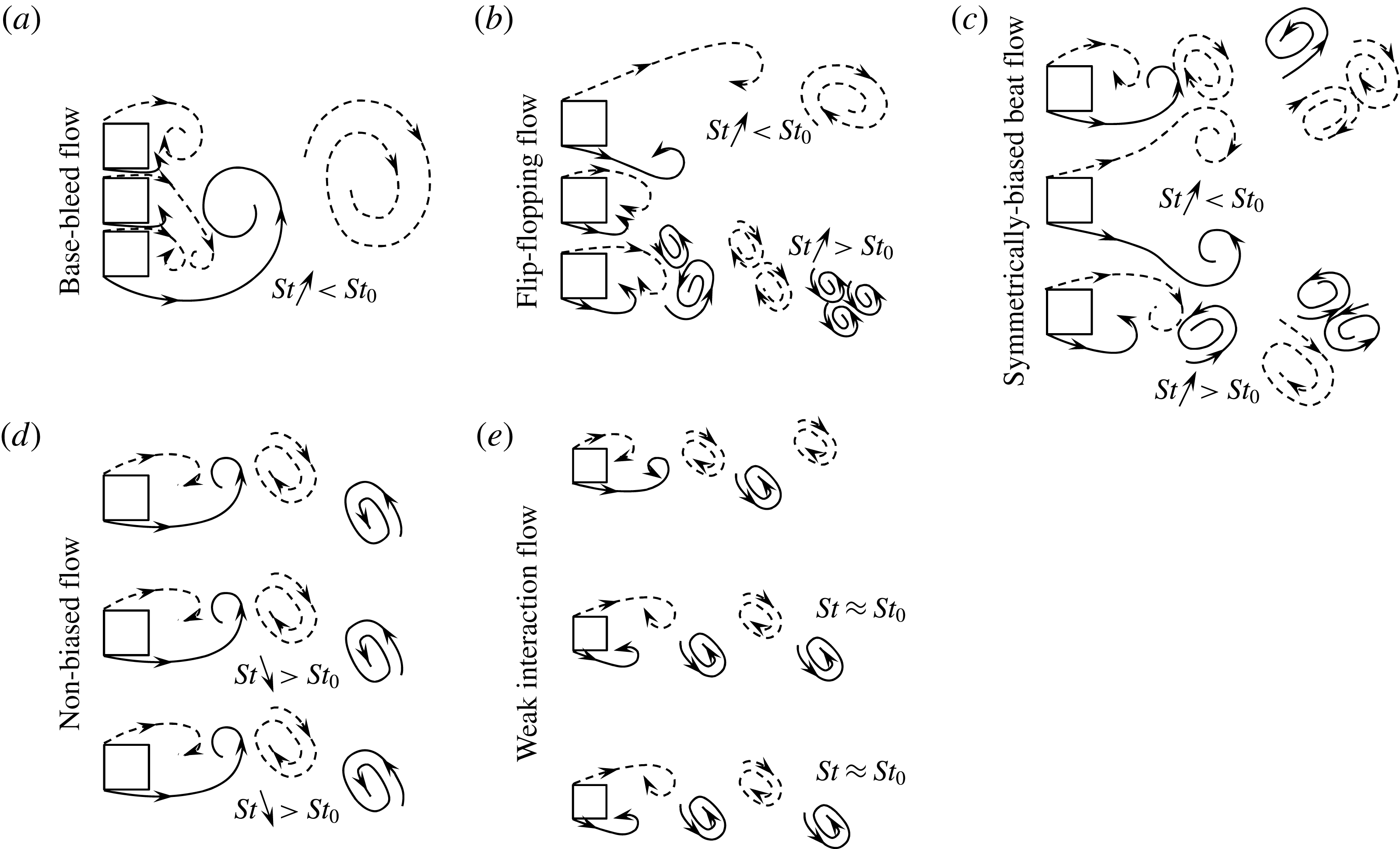
 $St$
also distinguishes the flow regimes. Figure 16, as a recapitulation, presents sketches of flow structures at different regimes, showing the relationship between the shedding frequencies and their variations with
 $L/W$
, as discussed above. The up and down arrows indicate
 $St$
increasing and decreasing, respectively, with
 $L/W$
. Interestingly, each regime features distinct relationship and variations.
Sketches of flow structures, showing the behaviour of gap flows and vortex shedding. The relationship between the shedding frequencies and their variations are labelled in each wake. The up and down arrows indicate
 $St$
increasing and decreasing, respectively, with
 $L/W$
.

4.7 Scaling of shedding frequency
Roshko (Reference Roshko1954) formulated a universal Strouhal number
 $St^{\ast }$
to scale the shedding frequency of various bluff bodies. He adopted the wake width
 $w$
(the lateral distance between the two free shear layers) and the time-mean velocity
 $\bar{u}_{b}$
at the boundary layer separation as the characteristic parameters to define
 $St^{\ast }$
, as
 $$\begin{eqnarray}St^{\ast }=\frac{f_{s}w}{\bar{u}_{b}}=St\frac{U_{\infty }}{\bar{u}_{b}}\frac{w}{W}.\end{eqnarray}$$
He obtained
 $w$
from notched hodograph method and
 $\bar{u}_{b}$
from the base pressure
 $C_{pb}$
as
 $$\begin{eqnarray}\frac{\bar{u}_{b}}{U_{\infty }}=\sqrt{1-C_{pb}}.\end{eqnarray}$$
The
 $St$
in the range of 0.1330–0.2120 for different bluff-body shapes collapsed to a fairly constant value of
 $St^{\ast }=0.1630\pm 0.010$
. Griffin (Reference Griffin1978) defined the wake width as the lateral distance between two peaks in fluctuating (r.m.s.) velocity contours in the wake of a vibrating cylinder and packed up
 $St=0.1900{-}0.2100$
into
 $St^{\ast }=0.1820\pm 0.0080$
. It would be worth applying Roshko’s theory for multiple bodies where fluid–structure interaction is more complex.
Following Griffin’s definition of wake width and
 $\bar{u}_{b}$
estimated from
 $C_{pb}$
,
 $St^{\ast }$
for the three individual prisms is presented as a function of
 $L/W$
(figure 15
a). In regimes
 $D$
and
 $E$
,
 $St=0.1580{-}0.1870$
collapses to a fairly constant value
 $St^{\ast }=0.1240\pm 0.0030$
, very close to the
 $St^{\ast }$
of the single isolated prism
 $(St^{\ast }=0.1250)$
. However,
 $St^{\ast }=0.1250$
for the single isolated prism is different from
 $St^{\ast }=0.1820$
obtained by Griffin, which is attributed to the large difference between the present
 $(Re=150)$
and Griffin’s
 $(Re=450{-}2.47\times 10^{4})$
Reynolds numbers (Richter & Naudascher Reference Richter and Naudascher1976). In regime
 $C$
, the
 $St^{\ast }\;({\approx}0.2860)$
of the middle prism is far from the single isolated prism
 $St^{\ast }\;(=0.1250)$
, which insinuates that the definition of the universal Strouhal number does not fit for the symmetrically biased beat flow. The departure of
 $St^{\ast }$
for the middle prism in regime
 $C$
could be attributed to the very wide wake behind the middle prism
 $(w/W\approx 2.45)$
. Interestingly, the ratio of
 $St^{\ast }$
for the middle prism in regime
 $C$
to that for the single isolated prism is 2.29, close to the value of
 $w/W\approx 2.45$
. The remark reflects an indication that ignoring
 $w$
may provide a better collapse. In regime
 $B$
,
 $St$
has a band for both middle and outer prisms (figure 15
a). Here, for the sake of brevity,
 $St^{\ast }$
in this regime is based on the mid-value of the
 $St$
range.
 $St=0.1300{-}0.1540$
for the outer prisms and 0.1640–0.1760 for the middle prism collapse to
 $St^{\ast }=0.1070{-}0.1160$
and 0.1060–0.1310, respectively.
 $St^{\ast }$
of the three prisms does not collapse to a fairly constant value but nestles around that of the single isolated prism. The instability of the gap flow in regime
 $B$
might be the reason for the departure. In regime
 $A$
,
 $St=0.0470$
and 0.0610 at
 $L/W=1.1$
and 1.2 correspond to
 $St^{\ast }=0.1060$
and 0.1320, respectively. Apparently, the collapse of
 $St^{\ast }$
in regimes
 $A$
and
 $B$
is inferior to that in regimes
 $D$
and
 $E$
.
As discussed above,
 $w$
being large in regime
 $C$
may be responsible for the departure of
 $St^{\ast }$
, raising a question, can we ignore
 $w$
to formulate
 $St^{\ast }$
? In figure 15(b), we compare
 $\bar{u}_{b}^{\ast }\;(=\bar{u}_{b}/U_{\infty })$
and the maximum velocity in the shear layer
 $\bar{u}_{max}^{\ast }\;(=\bar{u}_{max}^{\ast }/U_{\infty })$
.
 $\bar{u}_{max}^{\ast }$
is the maximum time-mean streamwise velocity near the side surface of the prism, obtained from time-mean streamwise velocity contours. The
 $\bar{u}_{max}^{\ast }$
and
 $\bar{u}_{b}^{\ast }$
are not identical at a given
 $L/W$
, even at large
 $L/W$
(regime
 $E$
) or for a single prism, implying that the shear-layer velocity estimated from the base pressure does not reflect the actual velocity in the shear layer. In the previous works (Roshko Reference Roshko1954; Bearman Reference Bearman1967; Richter & Naudascher Reference Richter and Naudascher1976; Griffin Reference Griffin1978),
 $\bar{u}_{b}$
was estimated from
 $C_{pb}$
assuming that the Bernoulli equation can be applied to the flow around bluff bodies, and the pressure at the flow separation point and at the base is the same. Indeed, the real flow around a bluff body is viscous, and the pressure at the base and separation is not the same (e.g. Achenbach Reference Achenbach1968; Lee Reference Lee1975; Zdravkovich Reference Zdravkovich1997), consistent with that found presently for single and multiple square prisms. The departure between
 $\bar{u}_{max}^{\ast }$
and
 $\bar{u}_{b}^{\ast }$
is very large in regimes
 $A{-}C$
. Here, we estimated a modified Strouhal number,
 $St_{mod}=f_{s}W/\bar{u}_{max}=St/\bar{u}_{max}^{\ast }$
, i.e.
 $\bar{u}_{max}$
is considered as the characteristic velocity instead of
 $U_{\infty }$
to define the Strouhal number. The
 $St_{mod}$
results are presented in figure 15(a) to see their consolidation. It should be noted that at regime
 $A$
 $(L/W<1.4)$
, the characteristic height
 $W$
for
 $St_{mod}$
is chosen as the total height
 $2L+W$
, not
 $W$
, and
 $\bar{u}_{max}$
on the free-stream side shear layers from the outer prisms is adopted. It is interesting that, in regimes
 $A$
,
 $B$
,
 $D$
and
 $E$
, the collapse of
 $St_{mod}$
and
 $St^{\ast }$
for both outer and middle prisms are similar. While
 $St^{\ast }$
for the middle prism is high
 $({\approx}0.2860)$
in regime
 $C$
,
 $St_{mod}$
for the middle prism is now
 ${\approx}0.1120$
, very close to that for the single isolated prism
 $(St_{mod}\approx 0.1190)$
. Strouhal number based on
 $\bar{u}_{max}^{\ast }$
provides better consolidation than that based on
 $\bar{u}_{b}^{\ast }$
, which suggests that
 $\bar{u}_{max}^{\ast }$
is the correct choice for the shedding frequency scaling.
(a) Lower and upper edges of lift signals of prisms 1 and 3, respectively, (b) lower edges of normalized streamwise velocity
 $u^{\ast }\;(=u/U_{\infty })$
at the upper and lower gap centres. The red dashed lines represent the trajectory of peaks. (c) Variation in
 $\unicode[STIX]{x1D703}_{u}$
and
 $\unicode[STIX]{x1D703}_{l}$
with time. See (d) for definitions of
 $\unicode[STIX]{x1D703}_{u}$
and
 $\unicode[STIX]{x1D703}_{l}$
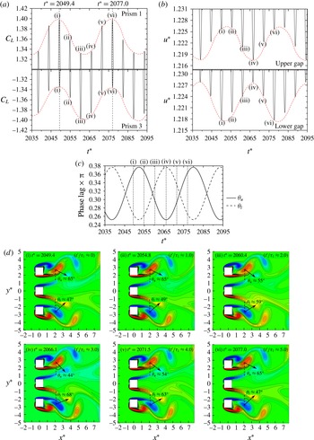
. (d) Contours of instantaneous vorticity field showing the phase lag between the vortex shedding from each gap. The instants of the fields are marked in (a).
 $t^{\prime }$
is the time delay measured from the instant (i) that corresponds to a
 $C_{L}$
peak of the prism 1, and
 $\unicode[STIX]{x1D70F}_{1}$
is the shedding period of the same prism. The angle between the line connecting the two vortex centres and the vertical direction represents the phase lag between the two vortices. Here
 $L/W=2.5$
.

5 Physics of the beat frequency and beat flow
From the power spectra results, it has been observed that
 $C_{L}$
signals at the symmetrically biased beat flow and non-biased beat flow regimes have a short (Strouhal or primary frequency) and a long (secondary frequency) period. The
 $C_{L}$
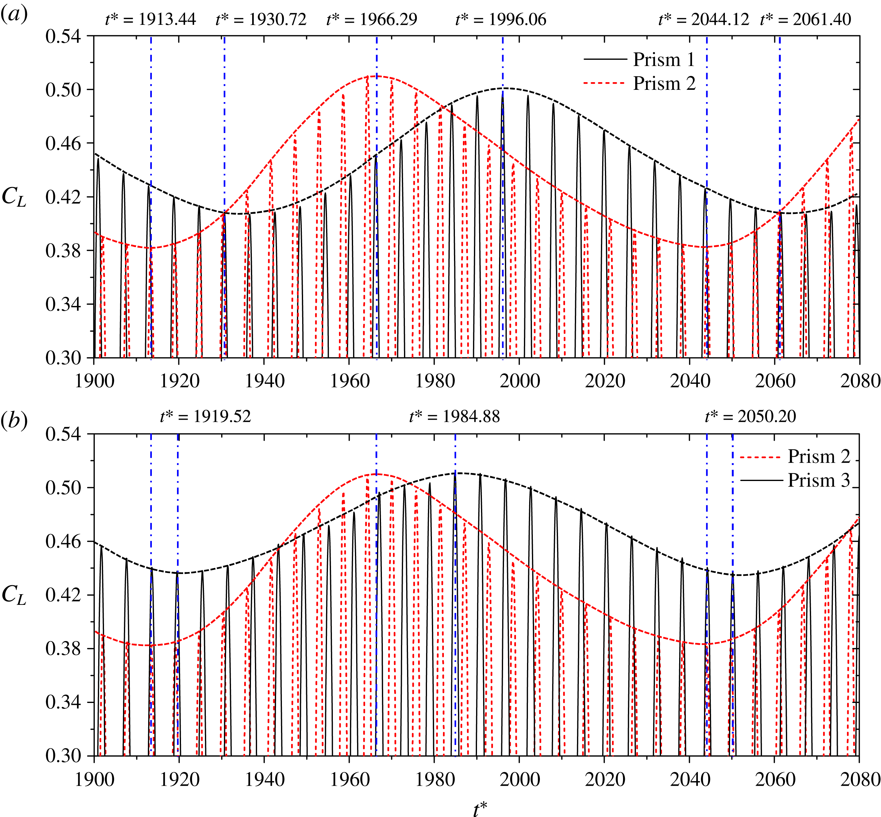
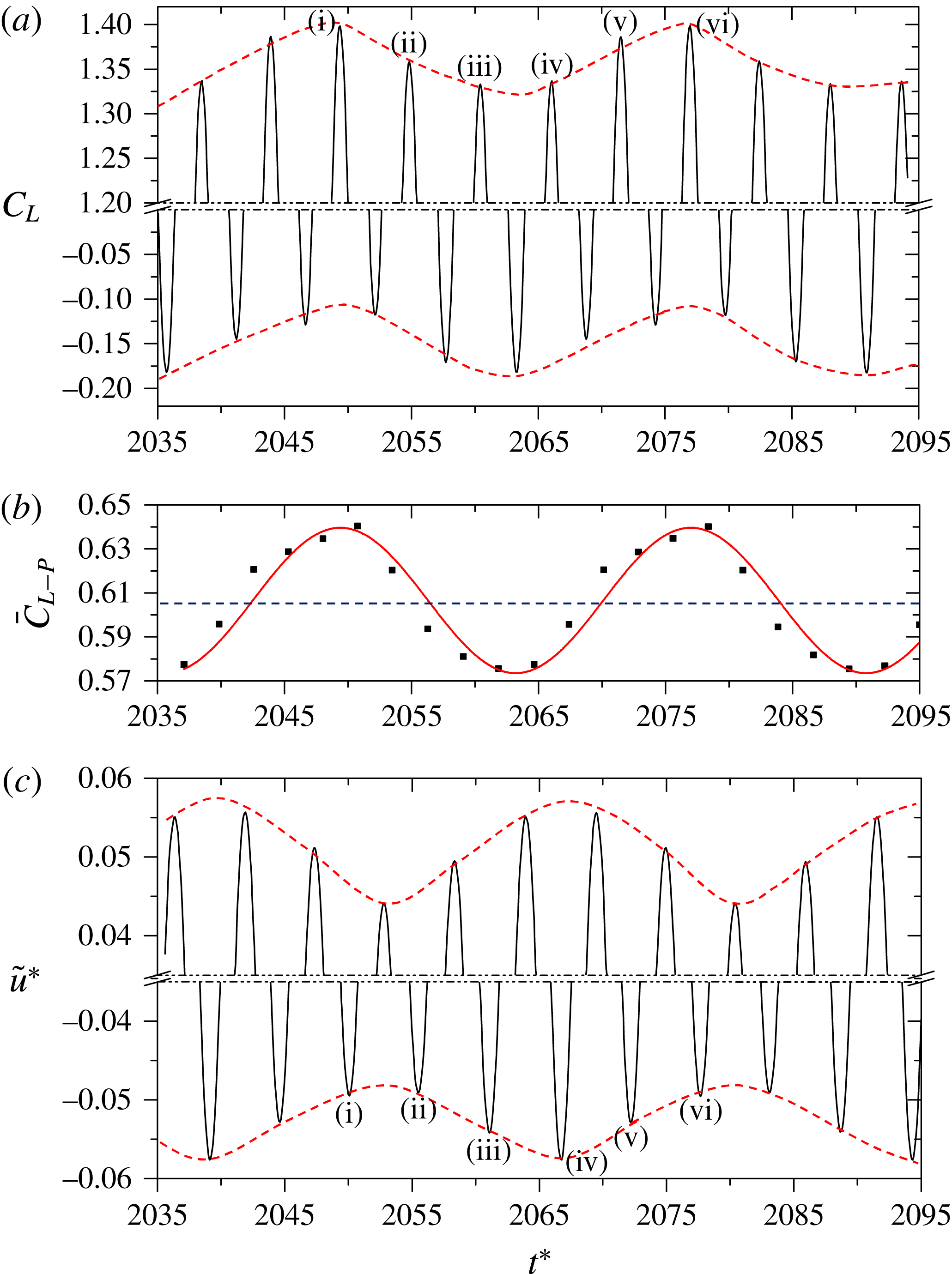
amplitude (or peak in the power spectrum) corresponding to the long period is small compared with that to the short period, as observed in figures 11(a,c) and 13(a,c). Figure 17(a) shows a zoom-in view of only the upper and lower edges of the
 $C_{L}$
signals of prisms 1 and 3, respectively, at
 $L/W=2.5$
, displaying more clearly the effect of the beat flow associated with the secondary frequency of the
 $C_{L}$
amplitudes. The short period is easily understood. A beat-like change in the
 $C_{L}$
peak for both upper and lower prisms is apparent, the upper and lower prisms corresponding to respectively a large and a small amplitude (peak) at
 $t^{\ast }=2049.4$
, a small and a large amplitude at
 $t^{\ast }=2060.4$
and again a large and a small amplitude at
 $t^{\ast }=2077.0$
. This gives a non-dimensional beat period of
 $T^{\ast }=27.6\;(=2077.0{-}2049.4)$
which corresponds to
 $St=0.0362$
, very close to the secondary frequency,
 $St=0.0360$
, obtained in the power spectra (figure 11
c). The discussion above and in § 4.4 thus corroborates that the beat phenomenon is associated with the secondary frequency, emerging from the instantaneous phase lag between the sheddings from the middle and outer prisms. As we know from sound/light interference, a beat occurs when two sound/light waves with different frequencies interact with each other and the beat frequency is equal to the difference between the two frequencies. Here, we observed the same phenomenon; the secondary or beat frequency is the difference in the shedding frequencies of the middle and outer prisms. The fundamental and important issues are: what are the origins of the secondary frequency and associated flow and how do they affect the lift acting on the prisms?
It is worth mentioning that Kumar et al. (Reference Kumar, Sharma and Agrawal2008), also in a row of nine square prisms at
 $Re=80$
, observed the secondary frequency in the time histories of lift and drag signals at their quasi-periodic flows I
 $(4.0\leqslant L/W\leqslant 5.0)$
and II
 $(2.0<L/W<4.0)$
. They believed that the secondary frequency originates from a periodical/successive switch between narrow and wide wakes behind the middle and adjacent prisms. However, their explanation of the secondary frequency is not consistent with other aspects of the flow structures. At least two questions can be raised on this issue. Firstly, they believed that when a wide wake is formed behind the middle prism, a narrow wake accompanies the adjacent prisms and vice versa; and the two modes have their interchange in a continuous manner, widening or narrowing, respectively, at the period of the secondary frequency. If so, the adjacent and the middle prisms should have the same Strouhal frequency with a wide band in their power spectra of the lift signals; but the Strouhal peaks for the middle and adjacent prisms were sharp, appearing at two frequencies, respectively. Furthermore, the narrow and wide wakes always correspond to different shedding frequencies; then, how can the vortex sheddings from the middle and adjacent prisms have a definite phase lag at the quasi-periodic flow-I, as presented in their paper? Secondly, they noted that the switch (the secondary frequency) between the wakes was periodic at the quasi-periodic flow-I, but not at the quasi-periodic flow-II. If so, how does the secondary frequency of
 $St=0.0120$
emerge in the power spectra of the drag signal at
 $L/W=3.0$
? The above points indicate that the origin of the secondary frequency has not been well understood.
6 The origin of the secondary frequency and its effect on lift force
As discussed in § 5, the phenomenon of secondary frequency was observed in the symmetrically biased and non-biased beat flow regimes and linked to the beat-like change in
 $C_{L}$
peak or amplitude. However, the flow structures at both flow regimes are significantly different. In this section, we will reveal the origin of the secondary frequency and its effect on
 $C_{L}$
in the symmetrically biased and non-biased beat flow regimes in §§ 6.1 and 6.2, respectively, and clarify the intrinsic and common points of them in § 6.3.
6.1 Symmetrically biased beat flow
 $C_{L}$
amplitudes (
 $C_{L}$
-peak) of the two outer prisms (associated with the primary frequency) are always opposite to each other (figure 17
a), which demonstrates that the sheddings from the outer prisms are antiphase. A periodical change in
 $C_{L}$
-peak of either prism, following the secondary frequency, is obvious. When the
 $C_{L}$
peak of the upper prism reaches its maximum, that of the lower prism obtains its minimum and vice versa. But what makes the change in the
 $C_{L}$
peak? Figure 17(d) shows the shedding patterns at time instants marked by (i), (ii), (iii), (iv), (v) and (vi) in figure 17(a), where
 $C_{L}$
, associated with the shedding period (primary frequency), is maximum and minimum for the upper and lower prisms, respectively. At these instants, the phase lag between the two vortices from a gap can be defined by an angle
 $\unicode[STIX]{x1D703}$
between the line connecting the centres (maximum vorticity) of the two vortices and the vertical direction (figure 17
d).
 $\unicode[STIX]{x1D703}_{u}$
and
 $\unicode[STIX]{x1D703}_{l}$
stand for the phase lag in the upper and lower gaps, respectively. Interestingly,
 $\unicode[STIX]{x1D703}_{u}$
wanes gradually between instants (i) and (iv), and then increases between instants (iv) and (vi), with its maxima at instants (i) and (vi) and a minimum at instant (iv). The opposite variation prevails for
 $\unicode[STIX]{x1D703}_{l}$
. Comparing
 $\unicode[STIX]{x1D703}_{u}$
and
 $C_{L}$
peak (figure 17
a) variations, it is conspicuous that a larger
 $\unicode[STIX]{x1D703}_{u}$
corresponds to a greater
 $C_{L}$
peak of the upper prism.
 $\unicode[STIX]{x1D703}_{l}$
and the
 $C_{L}$
peak of the lower prism are correlated similarly. The observation implies that
 $\unicode[STIX]{x1D703}_{u}$
and
 $\unicode[STIX]{x1D703}_{l}$
are strongly connected to the variations in
 $C_{L}$
peak. As
 $C_{L}$
is the consequence of flow velocity around the prism, it is expected that
 $\unicode[STIX]{x1D703}_{u}$
and
 $\unicode[STIX]{x1D703}_{l}$
impact on the velocities in the corresponding gaps. While figure 17(d) provides some discrete values of
 $\unicode[STIX]{x1D703}_{u}$
and
 $\unicode[STIX]{x1D703}_{l}$
at some instants only, their variations with
 $t^{\ast }$
are presented in figure 17(c) for a couple of cycles. Obviously, the variations are sinusoidal, opposite to each other. The maximum and minimum values are
 $0.378\unicode[STIX]{x03C0}\;(=68^{\circ })$
and
 $0.245\unicode[STIX]{x03C0}\;(=44^{\circ })$
, respectively for either case.
Zoom-in views (only the lower edges of the signals) of
 $u^{\ast }$
histories at the upper and lower gap centres are shown in figure 17(b). An apparent relationship between the
 $u^{\ast }$
amplitude and corresponding
 $\unicode[STIX]{x1D703}_{u}$
or
 $\unicode[STIX]{x1D703}_{l}$
is observed; the smaller the
 $\unicode[STIX]{x1D703}_{u}$
or
 $\unicode[STIX]{x1D703}_{l}$
, the larger the corresponding
 $u^{\ast }$
amplitude and vice versa. The change of
 $\unicode[STIX]{x1D703}$
in a gap is connected to the difference in shedding frequencies between the middle and outer prisms. The physics behind the relationship between
 $\unicode[STIX]{x1D703}$
and
 $u^{\ast }$
will be given later.
6.2 Non-biased beat flow
Let us go back to figure 13(a) where a beat-like change in the
 $C_{L}$
amplitude was obvious. It is worth viewing representative flow structures at maximum and minimum amplitudes (associated with the secondary frequency) of the lift. The flow structures presented in figure 12 (i) and (iv) correspond to the maximum and minimum
 $C_{L}$
amplitudes (
 $t^{\ast }=$
1836.3 and 1877.4, respectively) associated with the secondary frequency, as indicated by vertical lines in figure 13(a). Interestingly, the maximum
 $C_{L}$
(figure 13
a) associated with the secondary frequency occurs when an in-phase shedding occurs from the two sides of a gap (figure 12
a (i)). On the other hand, an antiphase shedding from the two sides of a gap (figure 12
a (iv)) results in the minimum
 $C_{L}$
amplitude (figure 13
a). At this
 $L/W$
, both gaps simultaneously may have in-phase shedding (figure 12
a (i)) or antiphase shedding (figure 12
a (iv)), as the shedding phase lag between the outer prisms was a constant of
 ${\approx}0^{\circ }$
. The
 $C_{L}$
amplitudes of the three prisms thus reach their maxima or minima simultaneously. When the phase lag between the sheddings from the outer prisms is
 $\neq 0^{\circ }$
, maximum or minimum lift amplitudes of the outer prisms do not occur simultaneously. Zoom-in views of the
 $C_{L}$
signals of the three prisms at
 $L/W=5.0$
, where the phase lag between shedding from the outer prisms is approximately
 $0.21\unicode[STIX]{x03C0}({\approx}37.8^{\circ })$
, are presented in figure 18. The maximum
 $C_{L}$
amplitudes, associated with the secondary frequency, for the prisms 1, 2 and 3, occur at different instants, e.g. at
 $t^{\ast }=1996.06$
, 1966.29 and 1984.88, respectively (figure 18). So do the minimum
 $C_{L}$
amplitudes. The beat/secondary frequency thus results from a continuous change in the phase lag between the sheddings from the two sides of a gap, from in phase to antiphase, antiphase to in phase and so on. Furthermore, the change in the
 $C_{L}$
amplitude of the middle prism also depends on the phase lag between sheddings from the outer prisms. Due to the difference in shedding frequencies from the two sides of a gap, the instantaneous phase relationship changes in every primary period. When the shedding frequencies are different, how can the phase relationship be obtained? Here the phase relationship means the phase of the longer period shedding (outer prism) with respect to that of the shorter period shedding (middle prism), i.e. considering the shorter period as a reference complete cycle period.
Zoom-in views of lift signals of (a) prisms 1 and 2 and (b) prisms 2 and 3, at
 $L/W=5.0$
.

6.3 Effect on
$C_{L}$
of the phase lag between shedding from two sides of a gap

As discussed in §§ 6.1 and 6.2, the phase lag between the sheddings from two sides of a gap is closely connected to the variation in
 $C_{L}$
amplitude, and it is the generic origin of the secondary frequency. Here, the intrinsic relationship between the phase lag and
 $C_{L}$
acting on the prisms will be clarified, bridging flow structures and velocity and pressure fields. In one secondary period, the change in the phase lag between the sheddings from two sides of a gap is smaller at symmetrically biased beat flow than at non-biased beat flow; for example, the change is
 $44^{\circ }{-}68^{\circ }$
at
 $L/W=2.5$
(symmetrically biased beat flow, figure 17
d) and
 $0^{\circ }{-}180^{\circ }$
at
 $L/W=3.5$
(non-biased beat flow, figures 12
a and 13). The difference between the maximum and minimum
 $C_{L}$
amplitudes is thus smaller,
 ${\approx}0.064$
, at the former
 $L/W$
(figure 17
a) and larger,
 ${\approx}0.278$
, at the latter
 $L/W$
(figure 13
a). For a detailed discussion,
 $L/W=3.5$
is taken to be an exemplification of both beat flows.
As already discussed, in non-biased beat flow, the phase lag largely influences
 $C_{L}$
amplitude varying from a maximum to a minimum and vice versa. The phase lag effect on the flow field or
 $C_{L}$
amplitude variation can be understood from an instantaneous fluctuating field obtained from the instantaneous field minus the mean field, for instance, instantaneous fluctuating streamwise velocity
 $\tilde{u} ^{\ast }=u^{\ast }-\bar{u}^{\ast }$
and instantaneous fluctuating pressure coefficient
 $\widetilde{C}_{p}=C_{p}-\overline{C}_{p}$
, where
 $u^{\ast }$
(and
 $C_{p}=2p/\unicode[STIX]{x1D70C}U_{\infty }^{2}$
) and
 $\bar{u}^{\ast }$
(and
 $\overline{C}_{p}$
) are the instantaneous and time-mean streamwise velocities (and pressure coefficients), respectively.
(a,b) Contours of fluctuating streamwise velocity
 $\tilde{u} ^{\ast }\;(=u^{\ast }-\bar{u}^{\ast })$
around the prisms. (c,d) Distribution of fluctuating streamwise velocity
 $\tilde{u} ^{\ast }$
at
 $x^{\ast }=0$
and its gradient
 $\text{d}\tilde{u} ^{\ast }/\text{d}y^{\ast }$
with respect to
 $y^{\ast }$
. (e,f) Contours of fluctuating pressure coefficient
 $\tilde{Cp}=C_{p}-\bar{C_{p}}$
. (g,h) Sketches of flow structure. (i,j) Distribution of fluctuating vorticity flux
 $\tilde{u} ^{\ast }|\unicode[STIX]{x1D714}_{z}^{\ast }|$
at
 $x^{\ast }=0$
. The results in the first (a,c,e,g,i) and second (b,d,f,h,j) rows correspond to maximum and minimum
 $C_{L}$
amplitudes, respectively.
 $L/W=3.5$
. Note that
 $u^{\ast }=u/U_{\infty }$
;
 $C_{p}=2p/\unicode[STIX]{x1D70C}U_{\infty }^{2}$
. The solid and dotted lines represent positive
 $({\geqslant}0)$
and negative
 $({<}0)$
contour levels, respectively. The contour increment is 0.05.

Figure 19(a,b) at
 $L/W=3.5$
presents contours of
 $\tilde{u} ^{\ast }$
at instants (i) and (iv) (see figures 12
a, 13
a), corresponding to the maximum and minimum
 $C_{L}$
amplitudes associated with the in-phase and antiphase sheddings from each gap, respectively. The corresponding flow sketches are also given in figure 19(g,h). Similarly, contours of
 $\widetilde{C}_{p}$
conforming
 $\tilde{u} ^{\ast }$
contours are rendered in figure 19(e,f). Since
 $C_{L}$
of a prism is connected to the difference between the velocities (or pressures) over the two side surfaces of the prism, a clear view of velocities on side surfaces and in the gaps can be given by a
 $\tilde{u} ^{\ast }$
profile at
 $x^{\ast }=0$
, as presented in figure 19(c,d). In the same figure,
 $\text{d}\tilde{u} ^{\ast }/\text{d}y^{\ast }$
, which is an indication of shear stress, is also presented. To assimilate the
 $\tilde{u} ^{\ast }$
contours, let us first focus on the upper prism only (figure 19
a). As known, alternating Kármán vortex shedding results in an alternating flow on the two opposite sides of a body.
 $\tilde{u} ^{\ast }$
is positive and negative on the upper and lower sides, respectively (figure 19
a), with a hump on each side (figure 19
c) corresponding to the separated shear layer, indicating that at this instant the vortex from the upper side is developing and that from the lower is developed (see also figure 12
a (i)).
 $\widetilde{C}_{p}$
also communicates the above observation, negative and positive on the upper and lower sides of the prism, respectively (figure 19
e). It can thus be said that at this instant the fluctuating flow is positive (forward) on the upper side and negative (reverse) on the lower side of the upper prism.
Now we can move forward to discuss the physics the figure illuminates. The same, negative signed
 $\tilde{u} ^{\ast }$
in the upper gap suggests that the flow in the upper gap (across
 $x^{\ast }=0$
) is decelerating at this instant (figure 19
a,c,g), and the sheddings from the two sides have
 ${\approx}0^{\circ }$
phase lag (in phase). Similarly, the flow in the lower gap is accelerating with a
 $0^{\circ }$
phase lag between the sheddings from the two sides of the gap.
 $\widetilde{C}_{p}$
is thus positive and negative in the upper and lower gaps, respectively (figure 19
e). The two humps in
 $\tilde{u} ^{\ast }$
distribution in each gap (figure 19
c) represent two shear layers.
 $\text{d}\tilde{u} ^{\ast }/\text{d}y^{\ast }$
is small and asymmetrically distributed about the gap centrelines
 $y^{\ast }=\pm 1.75$
where
 $\text{d}\tilde{u} ^{\ast }/\text{d}y^{\ast }=0$
. In other words, the entire flow in a gap oscillates as an entity, of course, with a variation in
 $\tilde{u} ^{\ast }$
with
 $y^{\ast }$
, resulting in a maximum variation of
 $\tilde{u} ^{\ast }$
as well as
 $\widetilde{C}_{p}$
in one shedding cycle, hence in maximum
 $C_{L}$
amplitude. Furthermore, the oscillating flow in a gap is opposite to that in the other (figure 19
c), which also enhances the
 $C_{L}$
amplitude. This is why the antiphase shedding from the outer and middle prisms (in-phase shedding from the two sides of each gap) corresponds to maximum
 $C_{L}$
amplitude.
Oppositely, when the sheddings from the outer and middle prisms are in phase (figure 19
b,h),
 $\tilde{u} ^{\ast }$
values on the two sides of a gap are opposite to each other (figure 19
d,h). So are the
 $\widetilde{C}_{p}$
values (figure 19
f). That is, the vortex sheddings from the two sides of a gap occur with a phase lag of
 $180^{\circ }$
(antiphase). Here
 $|\text{d}\tilde{u} ^{\ast }/\text{d}y^{\ast }|$
is relatively larger and
 $\neq 0$
at the gap centrelines, but has an almost constant value for a range of
 $y^{\ast }$
near the gap centrelines (figure 19
d), suggesting that viscous force exists at the interface of the two sheddings from each gap. The viscous force restricts the momentum fluctuation through the gap during the vortex shedding, responsible for a faster decay of the gap vortices and vortex arrangement in the wake (figure 12
a (iv)). Furthermore, as the sheddings from the two sides of a gap are antiphase, the fluctuating streamwise velocity appears almost zero near the gap centrelines (figure 19
d), yielding a smaller oscillating flow in a gap than its counterpart in in-phase shedding (figure 19
c). A minimum variation in
 $\tilde{u} ^{\ast }$
or
 $\widetilde{C}_{p}$
thus prevails in one shedding cycle for this flow structure, corresponding to a minimum
 $C_{L}$
amplitude.
The vorticity flux across the gaps may reflect the lift forces on the prisms. The distributions of fluctuating vorticity flux
 $\tilde{u} ^{\ast }|w_{z}^{\ast }|$
at
 $x^{\ast }=0$
are presented in figure 19(i,j). Since a shear layer is characterized by large vorticity, the
 $\tilde{u} ^{\ast }|w_{z}^{\ast }|$
distribution displays a peak for each shear layer. The free-stream side shear layers correspond to a larger magnitude of
 $\tilde{u} ^{\ast }|w_{z}^{\ast }|$
than the gap shear layers. As the phase relationship changes from the in phase (figure 19
i) to the antiphase (figure 19
j), the peaks weaken not only for the gap shear layers but also for the free-stream side shear layers. That is, the difference in vorticity fluxes between the two sides of a prism for the in-phase shedding is greater compared to that of the corresponding prism for the antiphase shedding. The in-phase shedding thus leads to a maximum
 $C_{L}$
amplitude.
(a) Time history of the lift force on the upper prism (prism 1) and (b) normalized fluctuating streamwise velocity
 $\tilde{u} ^{\ast }=u^{\ast }-\bar{u}^{\ast }$
at the upper gap centre. Here
 $L/W=3.5$
. The red dashed lines represent the trajectory of peaks.

(a) Time history of lift force on the upper prism (prism 1). (b) Local mean lift
 $\overline{C}_{L-P}$
. (c) Normalized fluctuating streamwise velocity
 $\tilde{u} ^{\ast }$
at the upper gap centre. The red dashed lines represent the trajectory of peaks.
 $L/W=2.5$
.

The above discussion can be further fortified from simultaneous time histories of
 $C_{L}$
of the upper prism and of
 $\tilde{u} ^{\ast }$
at the upper gap centre (figure 20
a,b). It is apparent that the nature of signals shown in figure 20(a,b) is consistent with the above discussion. At
 $t^{\ast }=1836.3$
corresponding to the in-phase sheddings from the two sides of the gap, the amplitudes of
 $C_{L}$
and
 $\tilde{u} ^{\ast }$
associated with the secondary frequency are largest. Oppositely, at
 $t^{\ast }=1877.4$
corresponding to the antiphase sheddings from the two sides of the gap, the amplitudes of
 $C_{L}$
and
 $\tilde{u} ^{\ast }$
associated with the secondary frequency reach their minima. Between
 $t^{\ast }=1863.3$
and 1877.4, where the phase relationship between sheddings from two sides of the gap changes from in phase to antiphase, the extra viscous force acting on the interface of two sheddings grows from almost zero to a maximum, resulting in the amplitudes of
 $\tilde{u} ^{\ast }$
and
 $C_{L}$
altering from the maximum to the minimum. Accordingly, the overall flow undergoes a beat-like modulation. The contour of
 $\tilde{u} ^{\ast }$
peaks (red dashed line) on the upper side displays interruptions at
 $t^{\ast }\approx 1810$
and 1892 (figure 20
b). The interruptions occur when the phase lag between the vortex sheddings from the upper and middle prisms is approximately
 $0.5\unicode[STIX]{x03C0}$
(figure 13
b) with the upper prism shedding leading the middle prism. The condition corresponds to a phase lag of
 $-0.5\unicode[STIX]{x03C0}$
between the sheddings from the two sides of the upper gap. It is an orthogonal state of the two sheddings from the two sides of the upper gap; the influence of the shedding from the lower side to the shedding from the upper side is virtually zero. The
 $\bar{u}^{\ast }$
amplitude thus does not grow in this state. There is no interruption when the amplitude of
 $\bar{u}^{\ast }$
decays, e.g. between
 $t^{\ast }=1836.3$
and 1877.4. This might be connected to a fact that upper prism
 $St$
is smaller than the middle prism. A further in-depth investigation is required to unearth the detailed physics.
Unlike non-biased beat flow, where phase lag changes from in phase
 $(0^{\circ })$
to antiphase
 $(180^{\circ })$
, symmetrically biased beat flow is associated with a much smaller range of the phase lag between the sheddings from a gap, for example,
 $44^{\circ }{-}68^{\circ }$
at
 $L/W=2.5$
(figure 17). The modulation in
 $C_{L}$
amplitude is thus smaller as seen in time history of
 $C_{L}$
acting on the upper prism in figure 21(a). This history is reproduced from figure 11(a), showing the upper and lower peaks, in order to make the amplitude modulation visible. Local mean
 $C_{L}~(\overline{C}_{L-P})$
in each primary period is given in figure 21(b) to provide more information on the secondary variation in
 $C_{L}$
, where the solid points are the local mean, and the solid line is the fitting with a sine function, the dashed line being the averaged
 $C_{L}~(\overline{C}_{L})$
for the whole span of time. As discussed previously, the phase lag between the sheddings from the two sides of a gap influences
 $\tilde{u} ^{\ast }$
in the gap; the smaller the phase lag, the larger the
 $\tilde{u} ^{\ast }$
-amplitude. The
 $\tilde{u} ^{\ast }$
at the upper gap centre is presented in figure 21(c) to link the phase lag and
 $C_{L}$
. The amplitude of
 $\tilde{u} ^{\ast }$
is minimum around
 $t^{\ast }=2052.1$
and maximum around
 $t^{\ast }=2066.1$
, where the phase lag between the sheddings from the two sides of the upper gap is maximum and minimum, respectively (figure 17
d). The phase lag influence on
 $\tilde{u} ^{\ast }$
modulation can further be revealed from the fact that the modulation of
 $\tilde{u} ^{\ast }$
amplitude in one beat period is
 ${\approx}0.01$
(
 $=$
maximum amplitude minus minimum amplitude) at
 $L/W=2.5$
(figure 21
c) and
 ${\approx}0.06$
at
 $L/W=3.5$
(figure 20
b).
Furthermore, different from that in non-biased beat flow where
 $\overline{C}_{L-P}$
of outer prisms keeps constant,
 ${\approx}0.046$
for upper prism at
 $L/W=3.5$
(figure 20
a),
 $\overline{C}_{L-P}$
of the outer prism in symmetrically biased beat flow changes following the secondary frequency (figure 21
b). Evidently, the variation in
 $\overline{C}_{L-P}$
(figure 21
b) is connected to the shear-layer deflection, i.e. the phase lag,
 $\unicode[STIX]{x1D703}_{u}$
(figure 17
d), the larger the
 $\unicode[STIX]{x1D703}_{u}$
, the larger the
 $\overline{C}_{L-P}$
and vice versa. When
 $\unicode[STIX]{x1D703}_{u}$
grows, vortex
 $L_{1}$
leading
 $M_{1}$
to a greater degree (figure 10
a (i)) causes the two shear layers in the upper gap to be deflected upward to a greater extent (Alam & Zhou Reference Alam and Zhou2013). The wake centreline of the upper prism thus deviates from the nominal wake centreline to a greater degree, resulting in a larger repulsive force (i.e. a larger
 $\overline{C}_{L-P}$
). Oppositely, a smaller phase lag corresponds to a smaller repulsive force. As the phase lag between the sheddings from the two sides of the gap changes periodically sticking to the secondary period. So does
 $\overline{C}_{L-P}$
. Similar observation and conclusion were made for the lower gap and lower prism.
7 Conclusions
A detailed study has been conducted of the wake of three side-by-side square prisms for
 $L/W=1.1{-}9.0$
at a
 $Re=150$
. Based on vortex structures, gap-flow behaviours, fluid forces and shedding frequencies, five distinct flow regimes have been identified. (i) Base-bleed flow (regime
 $A$
,
 $L/W<1.4$
) is characterized by a single Kármán street, vortex shedding occurring from the free-stream sides only. Depending on the nature of the gap flows (weak or appreciable), base-bleed flow is further subdivided into two subregimes: weak base-bleed flow (
 $L/W\leqslant 1.1$
) and strong base-bleed flow
 $(1.1<L/W<1.4)$
. For the latter flow, the gap flows interacting with the free-stream side shear layers postpone the vortex formation length. The amplitude of the lift fluctuation is regular for weak base-bleed flow but irregular for strong base-bleed flow. (ii) Flip-flopping flow (regime
 $B$
,
 $1.4<L/W<2.1$
) refers to the gap flows flip flopping in a chaotic manner. The gap flows split the wake into three, and the three wakes transmute into one shortly, with the vortices from the gap flows decaying, merging and pairing with the free-stream side vortices. The lift force on each of the prisms is very chaotic. (iii) Symmetrically biased beat flow (regime
 $C,2.1<L/W<2.6$
) features the two gap flows deflecting outward symmetrically. The two vortices from a gap interact with each other and with the vortex from the respective free-stream side. The interaction, involving vortex integration and coupling, results in a beat-like modulation in the flow. The fluctuation in the lift for the middle prism is very small compared to that for the outer prisms. (iv) Non-biased beat flow (regime
 $D$
,
 $2.6<L/W<7.25$
) is exemplified by the fact that the gap flows are not biased anymore. An interaction of gap vortices of different frequencies results in a beat flow. The three prisms have almost the same fluctuation in the lift. (v) Weak interaction flow (regime
 $E$
) materializes at
 $7.25<L/W<9.0$
, where the beat phenomenon disappears and the interaction between the vortices from the gaps is insignificant. The amplitude and fluctuation in lift become regular.
The
 $St$
in base-bleed flow is small and identical for three prisms. While the effective
 $St$
for weak base-bleed flow is approximately equal
 $St_{0}$
, that for strong base-bleed flow is larger because a greater amount of opposite-sign vorticity, originating from the gap flows, expedites the vortex pinch-off process. At flip-flopping flow,
 $St$
is not identical for the three prisms, smaller for the outer prisms and higher for the middle prism. The correspondence of
 $St$
to the prisms switches in symmetrically biased beat flow, a smaller and a higher
 $St$
complementing the middle and outer prisms. The correspondence of
 $St$
to the prisms gets reversed in non-biased beat flow, where
 $St$
of the outer prisms is smaller than that of the middle prism. In weak interaction flow,
 $St$
of the three prisms is close to
 $St_{0}$
.
While in the literature Roshko’s (Reference Roshko1954) universal Strouhal number theory is validated for different shapes of isolated bluff bodies, nobody had attempted to validate Roshko’s theory for multiple bluff bodies, so far. Presently, the results for three side-by-side prisms validate the theory in non-biased beat and weak interaction flows, but not for base-bleed, flip-flopping and symmetrically biased beat flows, where the gap flows are biased and interact with free-stream side shear layers. Further research on this issue would be of interest.
The beat phenomenon or secondary frequency is observed in the symmetrically biased and non-biased beat flows, resulting from the difference in the shedding frequencies of the shear layers between the two sides of a gap. Due to the difference in the frequencies, the phase lag between the sheddings from a gap changes between a minimum and a maximum value following the secondary frequency. The phase lag has a great impact on the lift force; the smaller the phase lag, the larger the lift amplitude. The modulation of lift amplitude stems from the phase lag change. An in-phase (or smallest phase lag) shedding from a gap engender almost zero (or small) viscous force at the interface between the two shear layers from the gap, providing a larger momentum fluctuation through the gap in one shedding period, hence the greatest lift amplitude. On the other hand, an antiphase (or largest phase lag) shedding from the gap gives rise to a largest viscous force at the interface, restricting the momentum fluctuation through the gap, hence yielding a smallest lift amplitude.
Acknowledgements
M.M.A. wishes to acknowledge the support given by the National Natural Science Foundation of China through Grants 11672096 and from Research Grant Council of Shenzhen Government through grant JCYJ20160531191442288.