1. Introduction
We know that jet noise can be manipulated, enhanced or reduced, through a modification of the flow conditions in the vicinity of the nozzle exit. The modification may be due to a change in the geometry of the nozzle, using tabs or chevrons for instance (Zaman, Bridges & Huff Reference Zaman, Bridges and Huff2011) or non-circular nozzles (Gutmark & Grinstein Reference Gutmark and Grinstein1999). It may result from the addition of mass and momentum via steady-fluidic injection (Henderson Reference Henderson2010). However, the synthesis, and/or ‘optimisation’, of noise-reduction strategies remains problematic, being either guided by trial and error or based on the laborious exploration of hopelessly large parameter spaces. In the latter scenario, partial automation may sometimes be possible (Maury et al. Reference Maury, Koenig, Cattafesta, Jordan and Delville2012).
The limited success of noise-control strategies can be attributed to the lack of a solid conceptual framework connecting perturbations near the nozzle to the sound energy radiated to the far field, one that would enable a clear interpretation of the control effect, and thereby provide physics-based guidance through the myriad actuation possibilities.
Were it not for the fact that we know turbulent shear flows to comprise an underlying order, so-called ‘coherent structures’, or wavepackets, the establishment of such a connection would appear unimaginable. New numerical algorithms based on the iterative, forward and backward, solution of the Navier–Stokes equations and their adjoint do allow the sensitivity of the radiated sound to changes in the nozzle region to be established and exploited for control (Freund Reference Freund2001; Wei & Freund Reference Wei and Freund2006; Kim et al. Reference Kim, Kasnakolu, Serrani and Samimy2009). However, the cost of such computations is enormous, and their capacity to provide clear physical insight is confounded by the fact that the said connection is made through, and indeed hidden by, the chaotic motions of turbulence.
Wavepacket theory, the basis for which was laid in the 1960s and 1970s, is a simpler and yet pertinent means by which to establish a nozzle-to-sound connection that would guide jet-noise control. We here provide a very brief overview (for a more detailed treatment the reader is referred to the recent review of Jordan & Colonius (Reference Jordan and Colonius2013)), as this motivates the analysis methodology we pursue.
Following the observations of Mollo-Christensen (Reference Mollo-Christensen1963, Reference Mollo-Christensen1967), a large body of experimental, theoretical and more recently numerical work has been dedicated to the eduction of wavepackets from turbulence (Crow & Champagne Reference Crow and Champagne1971; Lau, Fisher & Fuchs Reference Lau, Fisher and Fuchs1972; Hussain & Zaman Reference Hussain and Zaman1981; Kerhervé et al. Reference Kerhervé, Jordan, Cavalieri, Delville, Bogey and Juvé2012), to their study as a sound-generation mechanism (Michalke Reference Michalke1970; Crow Reference Crow1972; Crighton Reference Crighton1975; Michalke & Fuchs Reference Michalke and Fuchs1975; Ffowcs-Williams & Kempton Reference Ffowcs-Williams and Kempton1978; Crighton & Huerre Reference Crighton and Huerre1990; Sandham, Morfey & Hu Reference Sandham, Morfey and Hu2006; Cavalieri et al. Reference Cavalieri, Daviller, Comte, Jordan, Tadmor and Gervais2011a , Reference Cavalieri, Rodriguez, Jordan, Colonius and Gervais2012b ; Kerhervé et al. Reference Kerhervé, Jordan, Cavalieri, Delville, Bogey and Juvé2012) and to their dynamic modelling (Michalke Reference Michalke1971; Liu Reference Liu1974; Crighton & Gaster Reference Crighton and Gaster1976; Tam & Morris Reference Tam and Morris1980; Mankbadi & Liu Reference Mankbadi and Liu1984). Eduction methodologies (e.g. Kerhervé et al. Reference Kerhervé, Jordan, Cavalieri, Delville, Bogey and Juvé2012) demonstrate the existence of low-amplitude organised motions, coherent over space and time extents that far exceed the integral scales of turbulence. Sound-source modelling confirms the assertion by Mollo-Christensen (Reference Mollo-Christensen1963) that these motions can generate a directive sound field – superdirective according to Crighton & Huerre (Reference Crighton and Huerre1990) and validated experimentally by Cavalieri et al. (Reference Cavalieri, Jordan, Colonius and Gervais2012a ) – due to an antenna effect (mutual interference between structures within the wavepacket). Modelling strategies, which have only recently been validated in a comprehensive manner (Gudmundsson & Colonius Reference Gudmundsson and Colonius2011; Cavalieri et al. Reference Cavalieri, Jordan, Colonius and Gervais2012a ; Rodrıguez et al. Reference Rodrıguez, Sinha, Bres and Colonius2013), show that these motions are synonymous with linear hydrodynamic instabilities of the turbulent mean flow. The scale separation between wavepacket motions and random background turbulence justifies such a use of the mean flow (Crighton & Gaster Reference Crighton and Gaster1976); the low fluctuation amplitude of wavepackets justifies the linearisation.
In unforced high-Reynolds-number turbulent jets, wavepackets are driven by in-flow perturbations associated with the nozzle boundary layer. The broadband character of these perturbations makes it difficult to establish a link between in-flow conditions and wavepacket evolution. The turbulent boundary layer is dominated by eddies of high azimuthal wavenumber that evolve into shear-layer turbulence of similar azimuthal structure. However, some small part of this structure drives low-order azimuthal modes in the jet; in addition to this azimuthal organisation, wavepackets are characterised by distinctive axial and radial organisations, and at any given axial location a specific preferred frequency can be observed in the spectrum (this is most clearly visible in the potential core and in the evanescent near pressure field). However, these wavepackets are clearly not harmonic, being driven by in-flow motions whose phase is stochastic.
Unsteady periodic actuation, on the other hand, produced for instance by fluidic pulsing (Maury et al. Reference Maury, Koenig, Cattafesta, Jordan, Delville, Bonnet and Gervais2009), plasma discharge (Samimy et al. Reference Samimy, Kim, Kastner, Adamovich and Utkin2007) or piezoelectric flapping (Butler & Calkins Reference Butler and Calkins2003), is a means by which perturbations may be imposed in a more controlled fashion at the nozzle: a well-defined frequency (i.e. with deterministic phase) and azimuthal mode combination can be introduced and the response of the flow (turbulence and sound) assessed with that knowledge. This is in contrast to the aforementioned steady-fluidic techniques, where the frequency–wavenumber structure of the near-nozzle perturbation is largely governed by the turbulence that results from the interaction between the main jet and the injected fluid.
In jets subjected to such harmonic in-flow forcing, wavepackets of different kinds may be present. The turbulent boundary layer continues to seed the flow with perturbations similar to the unforced case (provided that the actuation is such that the boundary-layer structure is not significantly modified), and so non-harmonic wavepackets similar to those of the unforced flow are possible; these will of course evolve differently if the mean flow of the forced flow differs from that of the unforced case. If the actuation is such that its (harmonic) frequency–azimuthal mode structure corresponds to an unstable shear-layer mode, harmonic wavepackets will arise and evolve with (superposed on) the stochastic wavepackets. In the case where actuation produces both harmonic and stochastic disturbances with frequency–wavenumber content to which the flow is unstable, harmonically and stochastically forced wavepackets will arise, in addition to the stochastic wavepackets driven by the boundary layer. The stochastic wavepackets due respectively to the boundary layer and the stochastic component of the forcing will, a priori, be indistinguishable; the harmonic wavepackets will, however, be identifiable due to their deterministic phase, and this fact will be exploited later in the paper.
A final component of the actuated flow that will be of importance in what follows is the turbulent response to actuation. Unsteadiness introduced by actuation, be it harmonic or otherwise, that has a frequency–wavenumber structure to which the flow is stable, will provoke the generation of turbulence not present in the unactuated flow. This turbulence will deform the mean flow, and thus modify the evolution of all wavepackets in the flow. This is a key idea in the analysis to follow.
In this sense, besides their practical interest, noise-controlled flows produced by unsteady actuation, be they louder or quieter, provide a useful setting for the testing of conceptual frameworks that would link actuation to sound. In this paper we present a novel actuator that produces an unsteady-fluidic perturbation in the near-nozzle region of a round jet. Depending on the frequency–wavenumber structure of the perturbation, the actuator can produce louder or quieter jets with respect to the baseline. The main contribution of this study is a rather complete analysis and interpretation of both control effects in terms of wavepacket theory.
The experiment and analysis methodology involve the introduction of perturbations dominated by azimuthal mode
 $m=2$
, over a range of frequencies, and a subsequent investigation of the response of the jet via triple decomposition of the velocity field. This permits eduction of the turbulence and phase-locked wavepacket components of the flow response as a function of actuation frequency. We then study the linear stability characteristics of the mean flows, the linear parabolised stability equations (PSE) being used to account for the slow divergence of the jets. The analysis is focused on azimuthal modes
 $m=0$
and
 $m=2$
. The former provides insight regarding changes in sound-source activity, while the latter is the key to understanding the control mechanism. A phenomenological interpretation of the controlled flows is thus proposed: actuation with an
 ${\it\omega}$
–
 $m$
organisation to which the mean flow is stable leads to the generation of a turbulence whose Reynolds stresses deform the mean flow such that the dynamics of the most acoustically efficient wavepackets are advantageously modified. This interpretational framework was first proposed by Gudmundsson & Colonius (Reference Gudmundsson and Colonius2007) and has subsequently been used by Sinha et al. to explain the effects of a different kind of fluidic actuator on the dynamics and sound-source mechanisms of turbulent jets; a significant reduction in phase velocity is identified as one of the decisive effects. A louder jet results when the flow is driven with an
 ${\it\omega}$
–
 $m$
structure to which the mean flow is unstable; in this case, nonlinear (quadratic) wavepacket interactions become relevant and increase the radiated sound.
This paper is organised as follows. In § 2 the experimental apparatus is presented and the measurement methodologies are outlined. Section 3.1 contains a description of the acoustic response of the flow to actuation. The main aerodynamic changes produced are described in § 3.2, and a more complete analysis of these and the acoustic results, with respect to the sound-source mechanisms, is performed in § 4, supported by PSE solutions. Some conclusions and perspectives are given in § 5.
2. Experimental set-up
The experiments were performed at the PPRIME Institute anechoic jet-noise facility, Bruit et Vent, at the CEAT, Poitiers, France. An isothermal jet issuing from a round nozzle with a plug is studied. The exit Mach number is varied from 0.3 to 0.6, but on account of limitations in the rotation speeds possible with the actuator, the main results reported here are for the
 $M=0.3$
case.
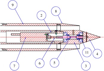
Sketch of the rotating plug mechanism, with the following parts highlighted: centreplug support (2), rolling bearing support (3), conical plug in PVC (4), crankshaft (5), heat shrink sleeve (6), Faulhaber 2057B electric motor (7), removable downstream nozzle (8), upstream nozzle (9) and seal (11).

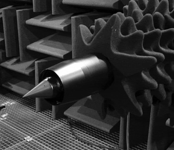
The nozzle and actuator are presented in figure 1. The main nozzle diameter is
 $D_{jet}=0.05~\text{m}$
; the actuator consists of a conical plug (centrebody) of diameter
 $D_{plug}=0.03~\text{m}$
and length
 $L_{plug}=0.046~\text{m}$
, mounted in the centre of the jet (see figure 2), and is driven in rotation by an electric motor. The air is ejected at
 $240~\text{m}~\text{s}^{-1}$
into the main jet by two diametrically opposed control ports of 0.0013 m diameter. The control-jet flow rate is less than 0.5 % of that of the main jet. This value is relatively low compared with those of other fluidic injection studies aimed at jet-noise reduction (see Henderson (Reference Henderson2010) for an exhaustive list), particularly for a turbulent jet. The study of the effects of different flow rates is currently an ongoing project by this group, and it will be important if the actuator proves to be effective at higher Mach numbers, which would make it viable for industrial applications. An attempt to ascertain how plug rotation alone, without fluidic injection, influences sound radiation was attempted; however, no broadband effect was seen in the acoustic field. This is consistent with the fact that, for the rotation speeds considered, the jet does not correspond to one with significant swirl (Kœnig Reference Kœnig2011).
An equivalent diameter,
 $D$
, is defined as
 $$\begin{eqnarray}D=\sqrt{D_{jet}^{2}-D_{plug}^{2}}=0.04~\text{m}.\end{eqnarray}$$
This diameter is used as the reference length of the flow and gives a Reynolds number of
 $Re_{D}=U_{j}D/{\it\nu}=2.7\times 10^{5}$
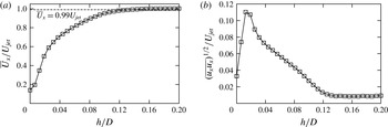
. The area contraction of the nozzle is 31. This convergent section is followed by a straight annular section of 150 mm length. A boundary-layer trip was used to force transition to turbulence 135 mm upstream of the nozzle exit. No boundary-layer trip was placed on the plug support. Hot-wire measurements were performed to measure velocities in the jet exit plane. Results for the mean and r.m.s. profiles are shown in figure 3. The boundary-layer characteristics obtained are typical of a turbulent case (Bridges & Hussain Reference Bridges and Hussain1987; Cavalieri et al.
Reference Cavalieri, Rodríguez, Jordan, Colonius and Gervais2013).
Rotating plug actuator in ‘Bruit et Vent’.

Microphone measurements were made at
 $30D$
from the jet, at downstream polar angles of 20° and 30°. For these shallow angles most of the acoustic radiation is related to wavepackets in the jet (Jordan & Colonius Reference Jordan and Colonius2013). A moving average was used to smooth the spectra, and peaks associated with sound radiated by the electric motor have been removed by a notch filter in the results presented here. Measurement of the broadband baseline spectra showed a repeatability with less than 0.5 dB deviation for experiments performed with a six-month time separation.
Boundary-layer profiles at the nozzle exit for a Mach 0.3 jet: (a) mean velocity; (b) r.m.s. value.

Velocity measurements were made using a LaVision time-resolved stereoscopic particle image velocimetry (hereafter TR-PIV) system and cameras with
 $1024~\text{pixel}\times 1024~\text{pixel}$
resolution. The light source was a 10 mJ Quantronix Darwin duo laser (light sheet thickness 2 mm) and the flow was seeded with oil smoke. Three components of velocity were measured in
 $r$
–
 ${\it\theta}$
planes at a range of axial stations by two SA1 Photron cameras. The sampling frequency was
 $2.7~\text{kHz}$
. Ten thousand PIV image pairs were recorded, this being sufficient for convergence of first- and second-order statistical moments. Image processing consisted of a five-pass correlation routine with
 $64~\text{pixel}\times 64~\text{pixel}$
correlation for the first pass,
 $16~\text{pixel}\times 16~\text{pixel}$
for the final pass and with a 50 % correlation overlap at each pass. The spatial resolution was one velocity vector every 0.75 mm for the small window size (near the jet exit) and one velocity vector every 1.5 mm for the large window size (around the end of the potential core). Hot-wire measurements are also presented in this paper to study the mixing layer close to the plug extremity where it was not possible to obtain accurate PIV measurements due to the proximity of the nozzle and plug surfaces. We use a single hot wire (
 $2.5~{\rm\mu}\text{m}$
), sampled at 250 kHz. An in situ calibration of the hot wire is performed as in Tutkun et al. (Reference Tutkun, George, Foucaut, Coudert, Stanislas and Delville2009). The velocity is measured by the hot wire in
 $x$
–
 $r$
planes.
Due to the specificity of the actuator (unsteadiness introduced by rotation), the time-periodic disturbances are similar to those induced by a two-blade helix. Since the two microjets are nearly identical, the perturbation introduced by the actuator is dominated by an azimuthal mode 2, and by a microjet-passing frequency equal to twice the rotation frequency:
 $f_{p}=2f_{rotation}$
; we use this microjet-passing frequency to define a perturbation Strouhal number,
 $St_{p}=f_{p}D/U_{j}$
.
3. Control effects
3.1. In the sound field
The injection flow rate and plug rotation frequency are the two control parameters. These were assessed for different main-jet Mach numbers, and the analysis indicates that, while similar noise reductions are probable at higher Mach numbers, the rotation-frequency limit (beyond a certain rotation speed the device overheats due to friction between the various moving parts) constrains us to study a Mach 0.3 jet. We therefore focus on this jet, at a fixed injection flow rate, and we explore the acoustic response of the system as a function of the perturbation frequency, the far field being measured at a single point.
The time-periodic motion of the actuator generates tonal self-noise, predominantly at
 $St_{p}$
, but the jet is also excited at this Strouhal number, and the resulting coherent periodic motion also radiates tonal sound. One cannot easily distinguish the parts of the far-field sound corresponding to actuator self-noise and flow response at
 $St_{p}$
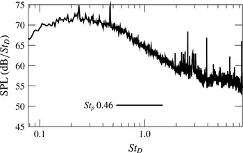
. Accordingly, for clarity, and similarly to other studies of periodically forced jets (Moore Reference Moore1977; Laufer & Yen Reference Laufer and Yen1983), a notch filter was applied in order to focus on the broadband response of the jet. The raw spectrum, prior to the filtering, is presented in figure 4, for the flow controlled at
 $St_{p}=0.46$
.
Acoustic spectrum prior to the filtering, for the
 $St_{p}=0.46$
controlled jet.

(a) Baseline and controlled noise spectra at 20° and Mach 0.3,
 $U_{mic}=240~\text{m}~\text{s}^{-1}$
; the perturbation frequencies are
 $St_{p}0.23$
and
 $St_{p}0.46$
. (b) Change in noise (contours in dB) as a function of the perturbation Strouhal number and Strouhal number.

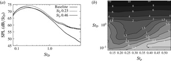
Once the acoustic spectra are smoothed by the notch filter, it is possible to evaluate more clearly the impact of actuation on the broadband sound. The result, summarised in figure 5, has three features of note. A high-frequency noise increase is observed at
 $St_{D}>2$
, where
 $St_{D}=fD/U_{jet}$
is the Strouhal number corresponding to a given frequency
 $f$
and
 $U_{jet}$
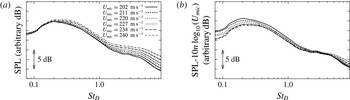
is the jet velocity. We associate this with scattering, by the plug, of turbulence associated with the interaction between the main- and control-jet flows: we have established that this component of the noise has a lower velocity scaling than the jet noise, and is no longer measurable at higher Mach numbers. This is shown in figure 6, where sound pressure spectra are shown with and without a velocity scaling (
 $U_{microjet}^{3}$
) based on the control-jet velocity. Other than jet interaction noise, a high-frequency penalty is expected due to the incoherent turbulence generated in the jet (Bridges & Brown Reference Bridges and Brown2004). Although it is currently impossible to separate the two contributions, as the speed of the microjets is increased, the former is expected to influence the total acoustic sound radiation less.
The second feature of interest is the monotonic increase, with perturbation frequency, of the crossover frequency between noise reduction and noise increase. Future studies, using a new, more rapid, prototype will establish whether this trend continues.
The third feature is the difference between the response of the jet to low- and high-frequency actuation. For low rotation speeds the acoustic radiation is increased, whereas when the rotation speed is increased there is a reduction of low-frequency sound. This is exemplified in figure 5 for two rotation Strouhal numbers. For
 $St_{p}=0.23$
there is a sound increase for all frequencies, and in what follows this flow will be labelled as the louder jet. On the contrary, for
 $St_{p}=0.46$
there is noise reduction for Strouhal numbers close to the peak radiation; accordingly, we label this as the quieter jet. In the following sections we study these two flows in some detail to get a sense of the mechanisms that lead to an increase or a reduction of the sound radiation.
Noise spectra at 30° and Mach 0.3 controlled at
 $St_{p}0.30$
with different microjet exit velocities (a) without velocity scaling and (b) with velocity scaling (
 $n$
exponent approximately 3).

Longitudinal evolution of (a) the mean axial velocity on the jet centreline, (b) the vorticity thickness and (c) the entrainment of the baseline and controlled jets at
 $St_{p}0.23$
and
 $St_{p}0.46$
.

3.2. In the aerodynamic field
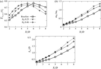
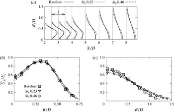
Some global indicators of the flow response to actuation are shown in figures 7 and 8. The mean-field deformation in the near-nozzle region is similar at both rotation frequencies, except on the centreline, where an increase in mean velocity is observed with increasing actuation frequency, indicating, incidentally, that a drag reduction may also result. Farther downstream, the low-frequency actuation leads to a significant reduction in mean centreline velocity; at the higher frequency a smaller reduction is observed. As the frequency is increased, the flow is thus seen to respond differently in the upstream and downstream regions. Figure 7(a) shows that in the near-plug region, as the actuation frequency is increased, the flow is progressively accelerated on the centreline; in the downstream region (
 $x/D>5$
), on the other hand, the flow undergoes a substantial deceleration in response to low-frequency actuation, a subsequent acceleration being observed as the actuation frequency is increased. We note, nonetheless, that the two controlled profiles have similar shapes: both entrain and redistribute axial momentum towards the centreline in the initial region. Such redistribution of axial momentum, with the flow being slowed down for positions close to the centreline, is also seen for large
 $r/d$
, as shown in figure 8. Both controlled flows have lower shear than the baseline jet. This is significant for the linear stability of the flow, as a reduction of the shear can be expected to favourably modify the dynamics of instability waves. This will be explored further in the next section.
(a) Mean axial velocity
 $\overline{U}_{x}/U_{j}$
; (b) zoom on radial profile at
 $x/D=2$
; (c) zoom on radial profile at
 $x/D=7$
.

(a) Turbulent kinetic energy profile; (b,c) zoom on radial profiles of turbulent kinetic energy for (b)
 $X=2D$
and (c)
 $X=7D$
.

The entrainment, shown in figure 7(b), is impacted in a similar manner at the two actuation frequencies up to
 $x/D=4$
, indicating that the higher centreline velocity observed in this region at the
 $St_{p}=0.46$
test point is due to redistribution rather than additional entrainment. Downstream of
 $x/D=4$
, it is the lower-frequency actuation that produces greater entrainment; we again note the non-monotonic character of this behaviour. Similar conclusions on the non-monotonic behaviour can be drawn by observing the vorticity thickness in figure 7(c).
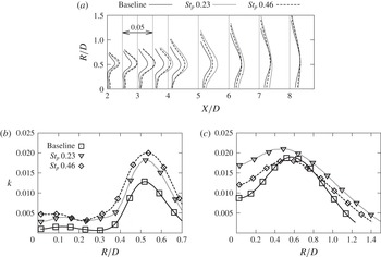
The turbulent kinetic energy, presented in figure 9, is similarly enhanced at both frequencies in the near-nozzle region, whereas downstream of
 $x/D=3$
, after a large increase at
 $St_{D}=0.23$
, it decreases at
 $St_{D}=0.46$
to the point where the peak levels drop below that of the baseline downstream of
 $x/D=6$
. The normal components of the Reynolds stress tensor (not shown) show a similar behaviour, indicating that the energisation is more or less isotropic.
In what follows, an analysis of the
 $({\it\omega},m)$
structure of the near-plug velocity field will help us to understand the very different axial evolutions of the fluctuation energy in the two cases: both flows are excited with the same amplitude, but with quite different spatiotemporal characteristics, provoking, as a consequence, quite different responses in the downstream region.
4. Analysis and interpretation
As discussed earlier, the modelling of wavepackets involves a linearisation of the Navier–Stokes system about the turbulent mean. Explicit nonlinear interactions between wavepackets are thus neglected. Nonlinearity is, however, implicitly present in the base flow, as this is established by Reynolds stresses associated with the nonlinearly interacting energy-containing eddies. Manipulation of these eddies can provoke a change in the Reynolds stresses, with which there will be an associated change in the mean flow, and, consequently, the dynamics of linear waves.
The following wavepacket characteristics are known to be important where their acoustic efficiency is concerned: (1) their fluctuation amplitudes, (2) the shape of their amplitude envelopes, (3) their phase velocities and (4) their ‘jitter’ (Cavalieri et al. Reference Cavalieri, Jordan, Agarwal and Gervais2011b ; Jordan & Colonius Reference Jordan and Colonius2013). The fluctuation amplitude cannot be directly obtained from a linear model, which involves a free constant that can only be determined by matching with experimental data; nor can wavepacket ‘jitter’ be usefully quantified by current linear models: this challenging issue is the object of ongoing research by this and other groups (Zhang et al. Reference Zhang, Towne, Jordan, Colonius and Lele2014, Reference Zhang, Tissot, Jordan, Lehnasch, Cavalieri, Colonius and Bres2015). On the other hand, information pertaining to the amplitude envelopes and phase speeds can be provided by linear theory. Locally parallel theory provides a first approximation of the growth rate at a given axial position, while PSE can be used to compute its axial evolution, taking into account the slowly varying change of the mean flow. Phase speeds can also be obtained, and we note that the dependence of sound radiation on this wavepacket parameter is exponential (Crow Reference Crow1972; Cavalieri et al. Reference Cavalieri, Jordan, Agarwal and Gervais2011b ).
We hypothesise that the quieter flow results from a modification of the mean flow, with which there is an associated change in acoustically relevant wavepacket dynamics, and we use linear theory to provide what information it can in this regard. A final caveat regarding linear theory is necessary before we proceed. A substantial body of work has been dedicated to its comparison with data issued from both experiment and computation. Until recently, these comparisons have shown compelling agreement in the Strouhal number range
 $0.3<St\leqslant 1$
; a more recent unpublished study by three of the present authors (Sasaki, Cavalieri & Jordan) has shown that this range can be extended to
 $0.3<St\leqslant 2$
. Linear theory does not show such good agreement at the lowest frequencies however, and this is a subject of ongoing study. The sound reductions we observe are in the range
 $St<0.3$
, i.e. in precisely that range where we cannot entirely trust growth-rate predictions. Only limited growth-rate results will therefore be presented in what follows, and these should be treated with caution, bearing in mind what we have said here. Phase velocities, on the other hand, are predicted with good accuracy over the entire spectrum of relevant frequencies (Gudmundsson & Colonius Reference Gudmundsson and Colonius2011; Breakey et al.
Reference Breakey, Jordan, Cavalieri, Léon, Zhang, Lehnasch, Colonius and Rodriguez2013). More solid conclusions that can thus be drawn when considering this wavepacket parameter, on which, as mentioned above, the sound field exhibits exponential dependence.
As discussed in the introduction, the rotating microjets lead to time-periodic fluctuations at the microjet-passing frequency, but also to broadband disturbances related to turbulence generated by the interaction between the control jets and the main jet. A priori both may lead to Reynolds stresses that affect the mean field, and hence the wavepacket dynamics.
A triple decomposition of the flow variables (Hussain & Reynolds Reference Hussain and Reynolds1970) is useful in this context. For the axial velocity component, for instance, we have
 $$\begin{eqnarray}u=\overline{U}+\tilde{u} +u^{\prime },\end{eqnarray}$$
where the axial velocity
 $u$
is written in terms of its mean value,
 $\overline{U}$
, a time-periodic component,
 $\tilde{u}$
, related to the rotating actuator, and a fluctuation,
 $u^{\prime }$
, that comprises both incoherent turbulence and non-periodic wavepacket motion.
4.1. The quieter flow: stabilisation of axisymmetric wavepackets
We first consider the quieter
 $St_{p}=0.46$
case, and note that the greatest noise reduction is observed at low emission angles, where the sound field is known to be predominantly axisymmetric (Juvé, Sunyach & Comte-Bellot Reference Juvé, Sunyach and Comte-Bellot1979; Kopiev et al.
Reference Kopiev, Chernyshev, Faranosov, Zaitsev and Belyaev2010; Cavalieri et al.
Reference Cavalieri, Jordan, Colonius and Gervais2012a
) and dominated by a source mechanism driven by the axisymmetric component of the axial velocity fluctuation (Michalke & Fuchs Reference Michalke and Fuchs1975; Cavalieri et al.
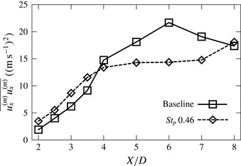
Reference Cavalieri, Rodríguez, Jordan, Colonius and Gervais2013). This sound source is considered by many (Jordan & Colonius Reference Jordan and Colonius2013) to comprise an axially extended non-compact wavepacket, understood as an instability of the mean field. We therefore examine the axial evolution of the fluctuation energy of the axisymmetric component of the velocity field, provided by a Fourier-series decomposition of the TR-PIV data and shown in figure 10. Reductions of up to 25 % are observed for the quieter flow downstream of
 $x/D=4$
.
Axial evolution of the fluctuating energy of the axisymmetric component of the axial velocity.

This reduction can be understood as due to a change in the dynamics of linear instabilities on account of a mean-field deformation produced by the actuation, which alters the growth rates and phase velocities of the fluctuations. A linear stability analysis using the measured mean velocity profiles is used to explore this assertion. We solve the linear PSE using the experimental mean flows from
 $x/D=2$
to 5 (sufficiently discretised mean-flow data were not available farther downstream). Details of the calculation and validation are given in the appendix A.
Let us first consider the growth-rate predictions. As the PSE includes the effect of mean-flow divergence, the growth rates are a function of radius and differ depending on the flow variable considered (Crighton & Gaster Reference Crighton and Gaster1976) (for further comments on the PSE, the reader is referred to the appendix A). We therefore consider the local wavenumber
 ${\it\alpha}(x)$
from the PSE ansatz,
 $$\begin{eqnarray}\boldsymbol{q}(\boldsymbol{x},t)=\hat{\boldsymbol{q}}(x,r)\,\text{e}^{\text{i}\int {\it\alpha}(x)\,\text{d}x}\,\text{e}^{\text{i}m{\it\theta}}\,\text{e}^{-\text{i}{\it\omega}t},\end{eqnarray}$$
which is responsible for the fast (i.e. exponential) axial evolution of disturbances within the jet. Accordingly, the imaginary part of
 ${\it\alpha}$
provides an average amplification throughout the flow and for all fluctuations. The changes for different flow quantities and radial positions are absorbed in the slowly changing function
 $\hat{\boldsymbol{q}}$
, and are less significant in comparison to the exponential growth in the integral of equation (4.2).
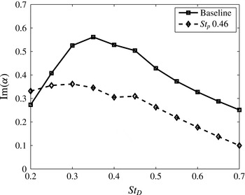
Figure 11 shows the PSE predictions for growth rates at
 $X=4D$
(i.e. towards the end of the region over which PSE computations were possible) in the baseline and ‘quiet’ flow. Substantial growth-rate reductions are manifested over a large frequency range, consistent with the experimental data presented in figure 10, which show suppressed fluctuation energy for azimuthal mode
 $m=0$
(integrated over all frequencies) downstream of
 $X=4D$
. This is an indication that the actuation has led to an acoustically useful mean-flow deformation where this wavepacket parameter is concerned.
Growth rates of the azimuthal mode
 $m=0$
at
 $X=4D$
, as a function of frequency, for baseline and
 $St_{p}=0.46$
actuation.

An average phase velocity,
 $U_{c}/c={\it\omega}/{\it\alpha}_{r}$
(with
 ${\it\alpha}_{r}$
corresponding to the real part of the wavenumber,
 ${\it\alpha}$
, and
 $c$
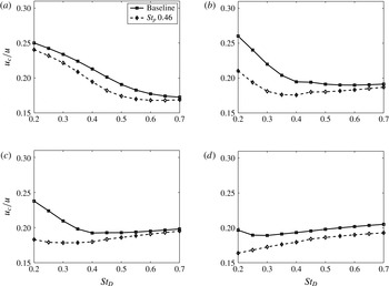
the ambient speed of sound), can also be defined. Figure 12, which presents the PSE predictions of phase velocity for the baseline and controlled flows at four axial positions, shows that the PSE predicts lower phase velocities for the actuated flow for all positions and frequencies considered. For the three most downstream positions the phase-velocity reduction is greatest at low frequency. As discussed earlier, this wavepacket parameter is known to be predicted with good accuracy by the PSE; it is a parameter on which the radiated sound depends exponentially. It is therefore probable that this modification is the most significant where the observed sound reduction is concerned.
Phase speeds predicted by the PSE for the baseline and controlled flows: (a)
 $X/D=2$
, (b)
 $X/D=3$
, (c)
 $X/D=4$
, (d)
 $X/D=5$
.

We have seen, using linear PSE results for the evolution of wavepackets, that the controlled jet has lower streamwise amplifications and phase velocities than the baseline case, which may explain the observed reductions in radiated sound. Since the predicted wavepackets are linearised solutions taking the mean field as the base flow, the differences must be related to changes in the mean flow. In what follows we examine the mechanisms that underpin mean-flow changes in the actuated jet.
The mean-flow deformation can be understood by considering the mean momentum balance for the axial velocity component, written in terms of a triple decomposition of the axial velocity,
 $u=\overline{U}+\tilde{u} +u^{\prime }$
,
 $$\begin{eqnarray}{\it\rho}_{0}\left(\overline{U}_{x}\frac{\partial \overline{U}_{x}}{\partial x}+\overline{U}_{r}\frac{\partial \overline{U}_{x}}{\partial r}\right)=-\frac{\partial \overline{P}}{\partial x}+{\it\mu}\overline{S}_{x}-{\it\rho}_{0}\left(\frac{\partial (\overline{\tilde{u} _{x}^{2}}+\overline{u_{x}^{\prime 2}})}{\partial x}+\frac{1}{r}\frac{\partial (r\overline{\tilde{u} _{x}\tilde{u} _{r}}+r\overline{u_{x}^{\prime }u_{r}^{\prime }})}{\partial r}\right),\end{eqnarray}$$
where
 ${\it\rho}_{0}$
is the density,
 $U_{x}$
and
 $U_{r}$
are the mean axial and radial velocity components,
 $P$
is the mean pressure field,
 ${\it\mu}S_{x}$
are the viscous forces along the axial direction,
 $u_{x}$
and
 $u_{r}$
are the axial and radial velocity fluctuations and
 $r$
is the radial distance.
Deformation of the mean field can be produced by both coherent and incoherent Reynolds stresses. The former is associated with a harmonic response of the flow to the harmonic component of the perturbations introduced by actuation, i.e. at
 $(St_{P},m)=(0.46,2)$
, while the latter is associated with non-harmonic components (e.g. small-scale structures generated as the exit flow interacts locally with the two wall jets). If the flow is unstable to the harmonic component of the actuation structure, the response will comprise harmonic wavepackets, phase-locked to the actuation; if it is unstable to any part of the stochastic component of the perturbations produced by actuation, stochastic wavepackets (difficult to distinguish from the wavepackets driven by the boundary-layer structure) will be produced; finally, if the jet is stable to both the harmonic and stochastic components due to actuation, wavepackets will not arise, and the response to actuation will comprise incoherent turbulence.
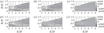
The triple decomposition allows identification of the contributions of the harmonic and stochastic components of the flow response to the Reynolds stresses that underpin the mean-flow structure. Figure 13, which shows the difference between the baseline and controlled-flow Reynolds stresses contributing to the streamwise momentum balance, indicates that the mean-flow deformation is dominated by the stochastic component of the Reynolds stresses. This demonstrates that the response of the flow to actuation is dominated by stochastic flow motions. That this is turbulence rather than stochastic wavepackets is suggested by an estimate of the characteristic frequencies associated with the local interaction between the exit flow and the two wall jets: vortex shedding from the wall jets (of diameter
 $d=0.0013$
) will occur at
 $St_{D}\approx 6.15$
; it is clear that the jet is stable to such a perturbation. This supports the contention that the response of the flow to the high-frequency actuation predominantly comprises turbulence rather than coherent structures.
Contribution of the non-cyclic and cyclic components in the Reynolds stress tensor comparatively to the baseline jet for
 $\overline{u_{x}^{\prime }u_{x}^{\prime }}$
(a–c) and
 $\overline{u_{x}^{\prime }u_{r}^{\prime }}$
(d–f): (a,d) total; (b,e) non-cyclic part; (c,f) cyclic part.

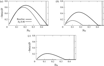
Growth rates of the azimuthal mode
 $m=2$
, as a function of frequency, for baseline and
 $St_{p}=0.46$
actuation: (a)
 $X=2D$
, (b)
 $X=2.5D$
, (c)
 $X=3D$
.

We now postulate that the dynamics of the flow response to actuation primarily comprises incoherent turbulence because the actuation energises the flow with an
 $({\it\omega},m)$
structure to which the mean field is stable. A linear stability analysis shows (cf. figure 14) that the mean field is indeed everywhere stable to the actuation structure
 $(St_{p}=0.46,m=2)$
, and so we conclude that the considerable fluctuation energy introduced into the system by the actuation at azimuthal mode
 $m=2$
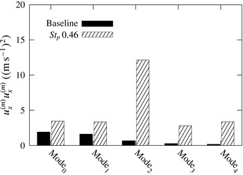
evolves downstream as incoherent turbulence, producing a mean-field deformation on which axisymmetric linear waves, which dominate downstream radiation, have lower growth rates and phase speeds than in the baseline flow. Figure 15 shows the considerable fluctuation energy introduced in the field at the
 $m=2$
mode; similar trends are seen in areas within the near-plug region of the jet (Kœnig Reference Kœnig2011).
With this we have a phenomenological interpretation linking the actuation to the far field. We note that the results of a number of other jet-noise control studies are consistent with this: noise abatement is most efficient when flows are driven with high
 ${\it\omega}$
–
 $m$
combinations (Samimy et al.
Reference Samimy, Kim, Kastner, Adamovich and Utkin2007; Kopiev et al.
Reference Kopiev, Chernyshev, Faranosov, Zaitsev and Belyaev2010). While we cannot affirm that the mean fields are in those cases stable to such actuation, this does seem likely, as the canonical mean field of a round subsonic jet is most stable to high frequencies and high azimuthal wavenumbers.
In the next section we consider the louder flow in a similar framework, but find that the behaviour is in this case fundamentally different.
Fluctuation energy of azimuthal modes of the axial velocity component in the near-plug region (
 $x/D=2$
) at
 $R=0.25D$
(where peak levels are observed).

4.2. The louder flow: nonlinear wavepacket dynamics
As an explanation for the different response of the flow to the actuation at
 $St_{p}=0.23$
, we postulate that this low-frequency actuation introduces high levels of fluctuation energy with an
 ${\it\omega}$
–
 $m$
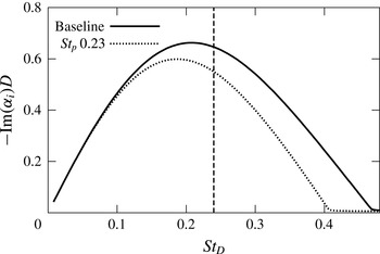
structure to which the mean field is unstable. This fact is confirmed in figure 16, which shows the results of a linear stability analysis, for the azimuthal mode
 $m=2$
, of both the baseline and actuated mean fields. In both cases, the actuation frequency lies close to the most unstable frequency of the mean field.
Consequently, coherent excitation at this
 ${\it\omega}$
–
 $m$
unstable pair would lead to exponential growth of disturbances at the excitation frequency, which would then lead to nonlinear interactions. The results suggest, furthermore, that when nonlinear wavepacket interactions are present in a subsonic jet, the radiated noise levels are increased above those of the canonical unforced flow.
Growth rates, at
 $x/D=2$
, as a function of frequency for the azimuthal mode
 $m=2$
, for baseline and
 $St_{p}=0.23$
actuation.

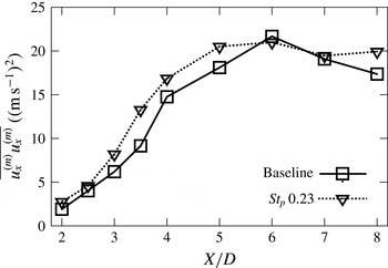
Figure 17 compares the fluctuation energy of the azimuthal mode
 $m=0$
between the baseline and louder flows. In this case we see a slight global increase of the latter. Application of the triple decomposition here shows, contrary to the
 $St_{p}=0.46$
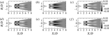
case, that most of the fluctuation energy is contained in the cyclic component. Figure 18, which shows six frames of the phase-averaged field over one complete period, reveals a pattern that repeats twice during that period: a frequency doubling appears to occur, indicating a quadratic wave interaction between the fundamental frequency and itself.
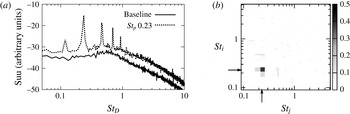
This is confirmed by analysis of hot-wire data. Figure 19(a) shows velocity power spectra of the baseline and controlled flows. These were measured at the centre of the mixing layer at
 $x/D=1.5$
. In the
 $St_{p}=0.46$
case a large spike is seen at the actuation frequency, but there are no harmonics. In the
 $St_{p}=0.23$
case, on the other hand, we see a large spike at the fundamental frequency, and this is accompanied by a series of harmonics. A bicoherence analysis shows (cf. figure 19) levels of over 40 % at
 $(St_{D},St_{D})=(0.23,0.23)$
, confirming that the first of these harmonics results from a nonlinear interaction of the fundamental with itself. The response of the flow to actuation at the lower frequency is thus seen to comprise nonlinear wavepacket dynamics, which are known to be considerably more efficient in the generation of low-angle sound (Suponitsky, Sandham & Morfey Reference Suponitsky, Sandham and Morfey2010).
Axial evolution of the fluctuating energy of azimuthal mode 0 for the axial velocity component.

Phase-averaged field of the axial cyclic component for the
 $St_{p}=0.23$
case. The phase is varying from
 $-\!{\rm\pi}$
to
 $2{\rm\pi}/3$
in steps of
 ${\rm\pi}/3$
: (a)
 $-{\rm\pi}$
, (b)
 $-2{\rm\pi}/3$
, (c)
 $-{\rm\pi}/3$
, (d) 0, (e)
 ${\rm\pi}/3$
, (f)
 $2{\rm\pi}/3$
.

(a) Hot-wire spectra in the mixing layer at
 $X=1.5D$
for the baseline jet and the controlled jets at
 $St_{p}0.23$
; (b) bicoherence in the mixing layer at
 $X=1.5D$
, showing nonlinear interaction of
 $St_{p}0.23$
with itself.

5. Conclusions
An experimental investigation of subsonic jets subjected to perturbations introduced by means of fluidic injection from a spinning centrebody has been performed. Fluctuation energy is introduced to the flow at the azimuthal mode
 $m=2$
(extension of this work to values
 $m>2$
is an ongoing project by this group, and preliminary results indicate similar trends) and over the perturbation Strouhal number range
 $0<St_{p}<0.5$
. At low frequency the acoustic response of the flow comprises a noise increase, while at higher frequencies peak noise levels are reduced. The louder and quieter flows are analysed and the mechanisms at work are shown to be quite different.
The control mechanism in the case of the high-frequency actuation involves the generation of incoherent turbulence and an associated change in the mean field. The latter comprises a reduction of mean velocity gradients, and this leads to a reduction of the growth rates and phase velocities of axisymmetric wavepackets – understood as linear instabilities of the mean flow and which are known to dominate low-angle emission. The mean-field deformation is shown, by a triple decomposition, to result from the energisation of incoherent turbulence, which arises because the high-frequency actuation introduces fluctuation energy with an
 ${\it\omega}$
–
 $m$
structure to which the mean field is stable.
The louder flow has velocity gradients similar to the high-frequency case, and therefore instability amplification rates and phase velocities of similar order. However, the actuation in this case is at frequencies to which the mean flow is unstable. Forcing in this manner leads to instability waves with initial amplitudes that are considerably greater than those of the unactuated flow, and which have a deterministic phase. Organised instability waves thus grow to a point where their amplitudes are large enough for significant nonlinear interactions to take place and dominate the flow dynamics: both the peaks and the broadband fluctuation levels are considerably enhanced and a louder jet results.
This study provides a demonstration of two very different kinds of control, and provides guidance for noise-control strategies. Actuators capable of producing mean-field deformations that lead to reduced shear have a good chance of producing a beneficial effect in terms of noise reduction by reducing the amplification rates and phase velocities of wavepackets – a mean-field effect. In the present work this deformation was shown to be due to the production of incoherent turbulent Reynolds stresses by forcing at stable
 ${\it\omega}$
–
 $m$
combinations. However, there are certainly other means by which such a mean-field deformation might be produced (simple changes in the nozzle geometry for instance). The control mechanism demonstrated in the case of the louder jet may also be of interest where noise control is concerned: forcing a jet at unstable
 ${\it\omega}$
–
 $m$
combinations can produce strong deterministic dynamics. While producing a louder jet in the present study, this kind of forcing is what is necessary for closed-loop control strategies, and, accompanied by a reduced-order model for the wavepacket dynamics (such as linear PSE), may allow for the real-time manipulation of the acoustic efficiency of sound-source dynamics, for the problem of jittering wavepackets for instance (Cavalieri et al.
Reference Cavalieri, Jordan, Agarwal and Gervais2011b
; Zhang et al.
Reference Zhang, Jordan, Lehnasch, Cavalieri and Agarwal2012).
Appendix A
The parabolised stability equations (PSE) apply to flows with mild streamwise variations, which allow for an extension of the parallel flow linear stability problem. In this case, the fluctuation term on the triple decomposition (4.1) is decomposed into a time-averaged axisymmetric component
 $\overline{\boldsymbol{q}}(\boldsymbol{x})$
and a time-dependent fluctuation
 $\boldsymbol{q}^{\prime }(\boldsymbol{x},t)$
, where
 $\boldsymbol{q}=[u_{x},u_{r},u_{{\it\theta}},{\it\rho},T]^{\text{T}}$
represents the flow variables (axial, radial and azimuthal components of velocity, density and temperature respectively) and cylindrical coordinates
 $\boldsymbol{x}=[x,r,{\it\theta}]$
are considered.
Given that the mean flow is homogeneous along the azimuthal and time directions, the fluctuation could be expressed in terms of normal modes in these directions,
 $$\begin{eqnarray}\boldsymbol{q}^{\prime }(\boldsymbol{x},t)=\mathop{\sum }_{{\it\omega}}\mathop{\sum }_{m}\tilde{\boldsymbol{q}}(x,r)\,\text{e}^{\text{i}m{\it\theta}}\,\text{e}^{-\text{i}{\it\omega}t},\end{eqnarray}$$
with
 $\tilde{\boldsymbol{q}}$
representing the complex amplitude for a given frequency
 ${\it\omega}$
and azimuthal wavenumber
 $m$
.
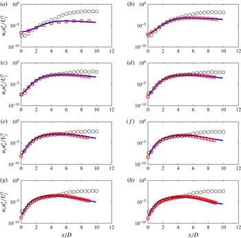
Centreline power spectral densities of the axial velocity – comparison between the implemented PSE method (squares) and data presented in Cavalieri et al. (Reference Cavalieri, Rodríguez, Jordan, Colonius and Gervais2013): earlier PSE calculation (solid line) and experimental values obtained from hot-wire measurements (circles), for (a)
 $St=0.2$
, (b)
 $St=0.3$
, (c)
 $St=0.4$
, (d)
 $St=0.5$
, (e)
 $St=0.6$
, (f)
 $St=0.7$
, (g)
 $St=0.8$
, (h)
 $St=0.9$
.

The solution may be further simplified by considering the wavepacket ansatz for slowly diverging jets (Crighton & Gaster Reference Crighton and Gaster1976):
 $\tilde{\boldsymbol{q}}(x,r)$
is decomposed into two separate contributions, a slowly varying function
 $\hat{\boldsymbol{q}}$
and a fast oscillatory function which captures the wave-like axial structure and the exponential amplification,
 $$\begin{eqnarray}\boldsymbol{q}^{\prime }(\boldsymbol{x},t)=\hat{\boldsymbol{q}}(x,r)\,\text{e}^{\text{i}\int ^{x}{\it\alpha}(x^{\prime })\,\text{d}x^{\prime }}\,\text{e}^{\text{i}m{\it\theta}}\,\text{e}^{-\text{i}{\it\omega}t},\end{eqnarray}$$
where
 ${\it\alpha}={\it\alpha}_{r}+\text{i}{\it\alpha}_{i}$
is the complex axial wavenumber, whose imaginary part will define growth or decay of disturbances along the axial direction.
By replacing the wavepacket ansatz (A 2) in the linearised, compressible Euler, energy and continuity equations, a matrix system is obtained,
 $$\begin{eqnarray}(A(\overline{\boldsymbol{q}})+B(\overline{\boldsymbol{q}},{\it\alpha},{\it\omega}))\hat{\boldsymbol{q}}+C(\overline{\boldsymbol{q}})\frac{\partial \hat{\boldsymbol{q}}}{\partial x}+D(\overline{\boldsymbol{q}})\frac{\partial \hat{\boldsymbol{q}}}{\partial r}=0,\end{eqnarray}$$
where the high Reynolds number of the flows considered justifies the neglect of the viscous terms. Linearisation allows the independent calculation of each
 ${\it\omega}$
–
 $m$
combination.
A second condition must be added to the PSE system (A 3) in order to eliminate the ambiguity between
 $\hat{\boldsymbol{q}}$
and
 ${\it\alpha}$
. This is done by forcing the spatial growth to be absorbed solely by the complex amplitude
 $\text{e}^{\text{i}\int {\it\alpha}(x^{\prime })\,\text{d}x^{\prime }}$
. This is ensured by the normalisation proposed in Herbert (Reference Herbert1997),
 $$\begin{eqnarray}\int _{0}^{\infty }\hat{\boldsymbol{q}}\frac{\partial \hat{\boldsymbol{q}\ast }}{\partial x}r\,\text{d}r=0.\end{eqnarray}$$
A pseudospectral method is used to discretise the radial derivatives, with functions described by means of Chebyshev polynomials. The axial derivatives are calculated using finite differences, and Dirichlet boundary conditions are used to define the flow variables at
 $r\rightarrow \infty$
.
The first step of the numerical method uses the parallel flow approximation to construct a spatial linear stability problem, whose solution gives the initial value to start the PSE iteration. Since these are solutions to linear PSE, they are determined up to a free constant, which is chosen so as to adjust overall amplitudes to experimental data.
Finally, the experimental data for the mean flow were fitted with a Gaussian profile in order to avoid non-smoothness of the experimentally obtained data.
Further comments on the PSE theoretical background and numerical approach that was chosen may be found in Herbert (Reference Herbert1997), Gudmundsson & Colonius (Reference Gudmundsson and Colonius2011), Rodríguez et al. (Reference Rodríguez, Cavalieri, Colonius and Jordan2015) and Sasaki (Reference Sasaki2014).
We now briefly present a validation of the numerical method used for solution of the PSE. Figure 20 presents the axial evolution of the fluctuation energy of the axisymmetric mode of the axial velocity for a turbulent jet of Mach 0.4 and Reynolds number
 $4.2\times 10^{5}$
. Results obtained using the present code are compared with the experimental and numerical data of Cavalieri et al. (Reference Cavalieri, Rodríguez, Jordan, Colonius and Gervais2013).
The PSE code used in this work closely reproduces the results of the calculation presented in Cavalieri et al. (Reference Cavalieri, Rodríguez, Jordan, Colonius and Gervais2013), thus validating the present method.
For the lowest frequencies, the PSE underestimate the growth of the fluctuations, which, while a known result (Gudmundsson & Colonius Reference Gudmundsson and Colonius2011; Cavalieri et al.
Reference Cavalieri, Rodríguez, Jordan, Colonius and Gervais2013; Sasaki Reference Sasaki2014), has not been clearly explained in the literature. For Strouhal numbers above 0.3, the PSE reproduce the behaviour of the velocity fluctuation correctly until the end of the potential core. After
 $X/D=5$
, the PSE no longer reproduce the experimental data, presenting an earlier saturation, indicating that linear wavepackets may no longer dominate the dynamics of the turbulent flow in this region.