





Impact Statement
Synthetic jets are widely deployed in applications ranging from flow control to laboratory turbulence generation, yet most designs rely on empirical tuning rather than predictive understanding. This work establishes a physical framework for multi-orifice synthetic jets by identifying the dominant flow regimes governing their downstream development and by quantifying how internal actuator geometry controls momentum transfer, jet merging and turbulence production. A key result is that orifice throat length – often treated as a secondary design detail – has a first-order impact on jet efficiency through its influence on exit velocity profiles. These insights directly inform the design of compact, energy-efficient actuators for flow control, thermal management and turbulence forcing, and provide a benchmark dataset for validating reduced-order and numerical models of synthetic jet arrays.
1. Introduction
Synthetic jets are used in various applications including convective heat transfer (Krishan et al., Reference Krishan, Aw and Sharma2019), turbulence generation (Nezami et al., Reference Nezami, Byron and Johnson2023), and flow control (Cattafesta & Sheplak, Reference Cattafesta and Sheplak2011). A synthetic jet is created by alternating blowing and suction motions through an orifice (Glezer & Amitay, Reference Glezer and Amitay2002), and the absence of external pumps and piping make synthetic jet actuators (SJAs) attractive actuators for flow control (Cattafesta & Sheplak, Reference Cattafesta and Sheplak2011).
A typical SJA consists of a cavity with an oscillating diaphragm on one side and an orifice on another side. As the diaphragm moves away from the cavity, it sucks fluid in through the orifice. During the opposite phase of the oscillation, the diaphragm then compresses the fluid in the cavity, creating a jet coming out of the orifice. For SJAs driven with a sinusoidal signal, the jet exit velocity is approximated by a sine wave. Such a sine wave can be characterised by various velocity scales. In the present work, we use
 $u_{\text{jet}}$
, equal to the maximum blowing velocity (i.e. the peak of the sine wave) as the characteristic scale. Other notable scales are a mean blowing velocity
 $\bar {u}_{\text{jet}} = u_{\text{jet}}/\pi$
(e.g. Smith & Glezer, Reference Smith and Glezer1998) and the momentum flow velocity
 $U_0 = u_{\text{jet}}/\sqrt {2}$
(e.g. Cater & Soria, Reference Cater and Soria2002), where the equalities result from assuming sinusoidal velocity cycles. The amount of expelled fluid is captured by the stroke length,
 $L_0=\bar {u}_{\text{jet}} T = \bar {u}_{\text{jet}}/f$
, where
 $T$
and
 $f$
are the period and frequency of the sinusoidal signal, respectively.
Whereas the time-averaged flow through the orifice is by definition zero-net mass flux, it leads to non-zero-net momentum flux at a distance
 $r$
away from the orifice due to the different development between suction and blowing phases. Suction through a single round orifice can be modelled as a sink which loses strength at a rate of
 $u\sim r^{-2}$
(Glezer & Amitay, Reference Glezer and Amitay2002). During the blowing phase the shear layers created at the orifice edge roll up into a vortex ring (alternatively, a vortex pair for a two-dimensional (2-D) orifice). This vortex ring propels itself linearly away from the orifice driven by its self-induced velocity (Auerbach, Reference Auerbach1987), focusing the momentum near the jet centreline. An important parameter for synthetic jets is the ‘formation criterion’
 $L_0/d\gt \pi$
, with
 $d$
the orifice diameter (Holman et al., Reference Holman, Utturkar, Mittal, Smith and Cattafesta2005), which measures whether the vortex is far enough away from the orifice to not be re-ingested during the subsequent suction cycle. For large enough
 $L_0/d$
, the vortex ring is moving away while the jet is still in its blowing cycle and a leading vortex ring can pinch off from the trailing shear layers. This occurs at a ‘formation number’ of
 $L_0/d=4$
(Gharib et al., Reference Gharib, Rambod and Shariff1998) such that for larger stroke lengths, a train of vortices is formed. At some point downstream, these vortices lose coherence and break down into a turbulent jet.
In various applications, the goal of an SJA is to inject mass, momentum or kinetic energy to the flow – in flux form scaling with
 $\rho A u$
,
 $\rho A u^2$
and
 $\rho A u^3$
, respectively. For a given velocity and near-constant density, these fluxes can be increased through the total orifice area
 $A$
. However, increasing the orifice diameter
 $d$
changes the jet formation dynamics, potentially pushing
 $L_0/d$
below the formation criterion. Alternatively,
 $A$
can be increased through the number of orifices while keeping
 $d$
constant. Such a multi-orifice synthetic jet (MOSJ) has potential benefits for multiple control goals by increasing the amount of injected mass, momentum and energy compared with a single orifice. In addition, the distributed forcing through multiple orifices may have benefits for heat transfer (Chaudhari et al., Reference Chaudhari, Puranik and Agrawal2011) and turbulence generation (Nezami et al., Reference Nezami, Byron and Johnson2023).
The implementation of multiple orifices introduces additional mechanisms that are not exhibited in traditional round jets. One that is critical in synthetic jet studies is the interaction between neighbouring vortex rings. Zhen-Bing & Zhi-Xun (Reference Zhen-Bing and Zhi-Xun2008) showed that neighbouring vortices coming out of side-by-side orifices have opposite circulation leading to destructive interference. For a pulsed jet (lacking a suction phase), Athanassiadis & Hart (Reference Athanassiadis and Hart2016) showed the same phenomenon and measured a minimum spacing of
 $\Delta /d \geq 3.5$
between neighbouring orifices such that each retains their single-jet momentum.
As multi-orifice arrangements are never perfectly axisymmetric, axis-switching is introduced to the flow. Cheng et al. (Reference Cheng, Lou and Lim2016) demonstrated that oblong vortex rings will deform out of plane and thus switch the major and minor axes. Similar behaviour has been documented for rectangular and generally non-circular orifices (Van Buren et al., Reference Van Buren, Whalen and Amitay2014). A centred hexagonal arrangement of orifices maximises symmetry (minimises axis switching) while ensuring one spacing parameter
 $\Delta$
applies to all inter-orifice distances (Goepfert et al., Reference Goepfert, Marié, Chareyron and Lance2010). This orifice geometry also maximises the packing density of orifices and will (presumably) lead to injection of the largest amount of energy and momentum.
Various studies used MOSJs for convective heat transfer (e.g. Chaudhari et al., Reference Chaudhari, Puranik and Agrawal2011; Kumar et al., Reference Kumar, Mirikar, Agrawal and Yadav2024; Mangate et al., Reference Mangate, Yadav, Agrawal and Chaudhari2019, and the recent review by Ahmed et al., Reference Ahmed, Ikhlaq and Arik2025) or turbulence generation (Goepfert et al., Reference Goepfert, Marié, Chareyron and Lance2010; Webster et al., Reference Webster, Brathwaite and Yen2004). Others investigated the development of dual-orifice synthetic jets (Kim et al., Reference Kim, Lee and Hwang2021; Palumbo & de Luca, Reference Palumbo and de Luca2021). However, to our knowledge, no fundamental investigations exist into the near- and far-field development of MOSJs from a single actuator.
To characterise the MOSJ parameter space, we divide it into three separate connected domains. First, the flow coming out of each individual orifice is equivalent to existing studies on synthetic jets. Assuming a sinusoidal signal and a circular orifice, the relevant non-dimensional parameters are the Strouhal number
 $St=fd/u_{\text{jet}}$
(or its inverse, the stroke length
 $L_0/d=\bar {u}_{\text{jet}}/(fd)$
) and a Reynolds number
 $Re=\rho u_{\text{jet}}d/\mu$
, where
 $\rho$
and
 $\mu$
are the density and viscosity, respectively (sometimes taken as
 $Re_{I_0}=I_0/(\rho d)$
with
 $I_0$
the momentum per unit width of the jet (Smith & Glezer, Reference Smith and Glezer1998)). Second, the use of multiple orifices requires definition of the geometry. As described earlier, a centred hexagonal pattern has optimal packing density and is defined by the number of rings around the central orifice (or, the number of orifices
 $N$
) in combination with the normalised inter-orifice (centre-to-centre) distance
 $\Delta /d$
. Third, while most studies on synthetic jets focus on the flow coming out of the orifice, the actuator geometry has several effects. These include overall performance due to the fluidic (or Helmholtz) frequency (Pierce, Reference Pierce2019) or necking (Jankee & Ganapathisubramani, Reference Jankee and Ganapathisubramani2019), both of which can be compensated by increasing the speaker power to provide a desired jet velocity at a given frequency. A more nuanced effect, which cannot be compensated for through the driving signal, is the effect of the orifice throat length
 $l_o$
on the jet exit velocity profile. A small aspect ratio
 $l_o/d$
leads to a top-hat (or constant) velocity profile with shear layers of negligible width, while large
 $l_o/d$
leads to a fully developed parabolic profile with thick shear layers. In the present work,
 $Re$
,
 $St$
,
 $\Delta /d$
and
 $N$
are kept constant while the often neglected
 $l_o/d$
is varied between cases to gauge its influence on the streamwise development of MOSJs. This streamwise development – specifically the merging of individual synthetic jets into a single merged jet – is the focus of the present work.
The outline of this paper is as follows: in §2, we outline our experimental methods; in §3, we present and discuss the obtained results; and finally, §4 presents our main conclusions.
2. Experimental methods
2.1. Description of the synthetic jet actuator
A Visaton KT-100 V 4
 $\Omega$
woofer loudspeaker is used as the driver for the synthetic jet actuator. This loudspeaker is rated for frequencies from 40 to 400 Hz with a rated power of 25 W. We use a Koolertron signal generator to drive the diaphragm with a sinusoidal signal of case-specific amplitude and frequency.
The loudspeaker is attached to two stacked 6.35 mm thick acrylic plates housing the laser-cut cavity and orifice, respectively. The cavity plate has a single circular through-hole of equal diameter as the speaker cone (92 mm). Four different interchangeable orifice plates are constructed with orifice diameters of
 $d=2$
, 3, 4 and 5 mm. Each orifice arrangement consists of a central orifice surrounded by a single ring of six orifices, each at a centre-to-centre distance of
 $\Delta /d = 3.5$
with respect to its neighbours.
For the orifice plate, the laser cutter is calibrated to minimise manufacturing artefacts like kerf and taper. The use of a laser cutter enables repeatable smooth throats. While laser cutting leads to a small fillet at the orifice edge, this fillet is orders of magnitude smaller than the orifice radius, such that the orifice can be approximated to have a sharp edge. The cavity and orifice plates are attached to the driver using nut and bolt hardware with an O-ring between the cavity plate and driver ensuring an airtight seal preventing leakage. The loudspeaker diaphragm itself acts as a seal between the cavity and atmosphere.
2.2. Measurement approach
We use particle image velocimetry (PIV) to quantify the flow outside the actuator in the streamwise–spanwise symmetry plane bisecting three of the seven orifices (i.e. the central orifice and two orifices located opposite from each other on the outer ring). We use a Quantronix Darwin Duo Nd:YAG dual pulse laser to illuminate fluid tracers that are seeded in the environment using a LaVision aerosol generator. LaVision's programmable timing unit (PTU) synchronises the laser pulses with two LaVision CX-5 cameras that take pairs of images with a case-dependent time delay between 4 and 20 µs. The cameras have a resolution of
 $2448\times 2048$
pixels and when using a 50 mm Nikon lens have a spatial resolution of
 $48.4 \times 40.5$
mm. Using DaVis 10, we compute velocity fields using one pass of a
 $64 \times 64$
pixel interrogation window with two subsequent passes at
 $32\times 32$
pixels with 50 % overlap. The cameras in 8-bit mode have a maximum frame rate of 54.5 Hz which we use to collect 2000 image pairs over
 ${\sim} 40$
s.
During postprocessing, we noticed a phase drift between the signal generator and the measurement system. To determine the relative phase of each velocity field, we perform a proper orthogonal decomposition, and use the time coefficients of the first and second modes to determine the relative phase (Pan et al., Reference Pan, Wang and Wang2013). The velocity fields are then averaged in batches of similar phase. Such phase averaging reduces measurement noise compared with single instantaneous velocity fields while retaining high temporal resolution.
2.3. Parameter space
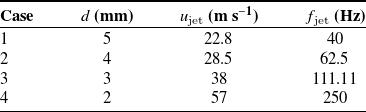
Four cases of varying orifice diameter are studied, where the frequency and velocity are tuned to keep
 $Re$
and
 $St$
constant, as summarised in table 1. Diameters are selected as discrete millimetre values between 2 mm, which is the smallest circular hole we could reliably manufacture, and 5 mm, beyond which the orifices get close to the edge of the actuator. Velocities are based on the highest velocity obtainable by the 2 mm actuator (
 $u_{\text{jet}}=57$
m s−1) with the other velocities determined by
 $Re$
-equivalence. Frequencies are based on the lowest reliable frequency of the loudspeaker (
 $f = 40$
Hz, below which its frequency response deteriorates) with the other frequencies based on
 $St$
-equivalence. To obtain the desired velocity at given frequency, the jets are calibrated by sweeping through different voltages at the set frequency. For each voltage, the velocity field above the central jet is captured using the described PIV set-up. As a characteristic jet velocity, we identify the maximum velocity for each voltage. This maximum always occurs at the centreline of the jet, but some distance away from the orifice. This offset distance is driven by the roll-up of the vortex ring outside the orifice edge (Smith & Glezer, Reference Smith and Glezer1998). We use this true maximum, not the maximum at the orifice, to define our jet velocity as it is easier to measure and more robust (Berk et al., Reference Berk, Hutchins, Marusic and Ganapathisubramani2018).
Physical parameter space for multi-orifice synthetic jet at
 $\Delta /d=3.5$
,
 $Re=7465$
and
 $St=0.0088$

Table 1 Long description
A table with four rows and four columns. The columns are labeled Case, d (mm), u_jet (m s^-1), and f_jet (Hz). The rows present the following data: Row 1: Case 1, d 5, u_jet 22.8, f_jet 40. Row 2: Case 2, d 4, u_jet 28.5, f_jet 62.5. Row 3: Case 3, d 3, u_jet 38, f_jet 111.11. Row 4: Case 4, d 2, u_jet 57, f_jet 250.
Prior studies have shown an influence of the number of orifices on the internal dynamics of SJAs (Chiatto et al., Reference Chiatto, Capuano and de Luca2018). For the purpose of the present work on the spatial development of MOSJ outside the actuator, the internal dynamics is of secondary importance and beyond the scope of the present study. Our actuator calibration minimises the influence of changes in actuator efficiency. For each case, we operate well below the predicted fluidic resonance frequency (predicted using a Lumped Element Model following Persoons, Reference Persoons2012), which minimises the influence of resonance on the output waveform.
The study of various cases with equal geometry and non-dimensional actuation parameters allows us to: (i) study the streamwise development of MOSJs and (ii) investigate the effect of physical dimensions of the actuator. The latter is not common in fluid dynamics when the focus is on the physics of the flow. However, it is of importance in the practical implementation, where a specific actuator needs to be used to generate the flow. This is not in contrast with the non-dimensional description; specifically, our results will show the importance of the orifice length
 $l_o$
, which is kept constant between our cases, but the varying aspect ratio
 $l_o/d$
alters the velocity profile at the orifice exit.
3. Results and discussion
3.1. Phase-averaged flow
Phase-averaged flow fields (indicated using
 $\widetilde {\cdot }$
) for the representative
 $d=3$
mm case are shown in Figure 1. Velocity fields are binned into 64 separate phases such that each field is averaged over
 $\Delta t = 1/64\,T\approx 0.016\,T$
, where
 $T$
is the period of the jet cycle. Figure 1a–d shows the streamwise velocity
 $\widetilde {u}/u_{\text{jet}}$
, highlighting the cyclic nature of the jets with peak blowing (panel b) and suction (panel d) phases. Three distinct jets are visible while two more jets are in front of the measurement plane and two behind the plane. Figure 1e–h shows the cross-flow velocity
 $\widetilde {v}/u_{\text{jet}}$
and Figure 1i–l the out-of-plane vorticity
 $\widetilde {\omega }_z/(u_{\text{jet}}/d)$
. Rather than the roll-up of a single vortex, the flow resembles long slugs of fluid as expected for our
 $St=0.0088$
corresponding to
 $L_0/d\approx 36$
, which is much larger than the formation number (Gharib et al., Reference Gharib, Rambod and Shariff1998). In panels d, h and l (
 $t/T=0.75$
), merging of the jets is visible at
 $x/d\approx 10$
. The streamwise component (panel d) forms one large puff rather than the three discrete puffs in panels a–c. Around the same location, the vorticity in panel l – while weak – is much stronger on the outside of the frame compared with in between the jets. This is as expected from inter-jet interactions where neighbouring positive and negative circulation cancels each other (Smith & Glezer, Reference Smith and Glezer2005).
Phase-averaged flow in the near-field for the
 $d=3$
mm case at
 $t/T \approx (\text{a, e, i})\,0$
; (b, f, j) 0.25; (c, g, k) 0.5 and (d, h, l) 0.75, corresponding to onset of blowing, maximum blowing, onset of suction and maximum suction, respectively. Rows show (a–d) streamwise component
 $\widetilde {u}/u_{\text{jet}}$
, (e–h) spanwise component
 $\widetilde {v}/u_{\text{jet}}$
and (i–l) out-of-plane vorticity
 $\widetilde {\omega }_z/(u_{\text{jet}}/d)$
.

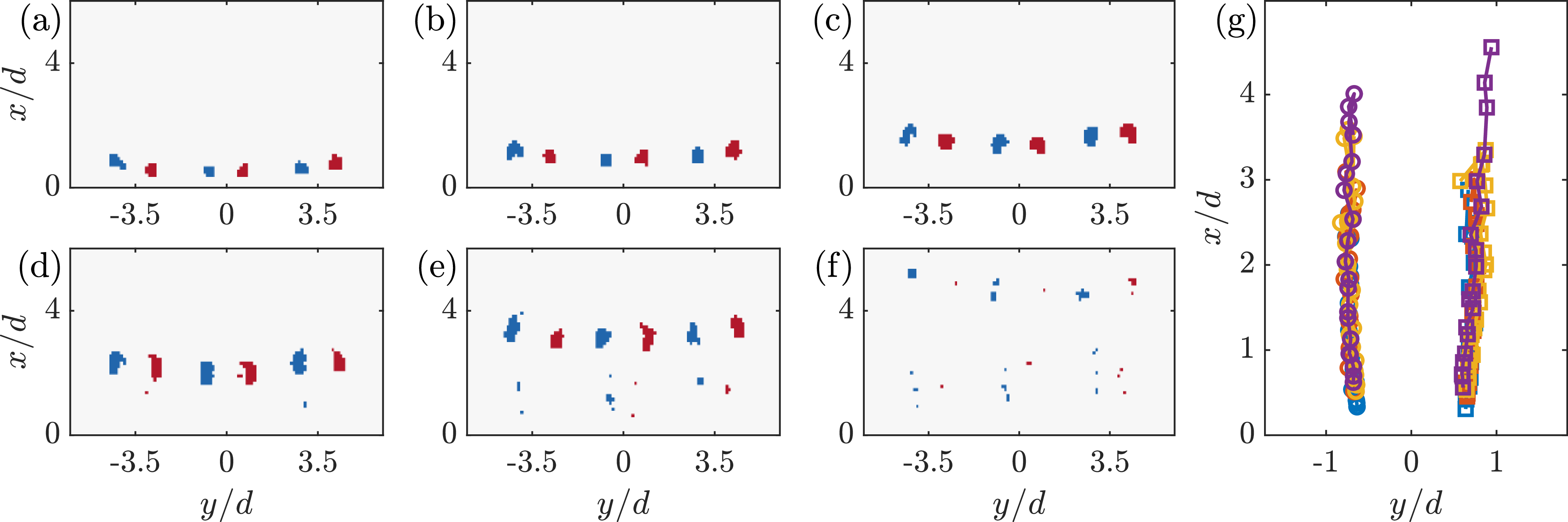
The leading vortex, visible in Figures 1i and 1j, can be separated from the trailing shear layer using a vortex identification method. Here, we use the swirling strength to identify vortices, which is defined as the imaginary part of the complex conjugate eigenvalues (
 $\lambda _{ci}$
) of the two-dimensional velocity gradient tensor (Adrian et al., Reference Adrian, Christensen and Liu2000). We then filter the vorticity field, retaining only regions where the swirling strength exceeds
 $\lambda _{ci}\gt 0.5 u_{\text{jet}}/d$
(where 0.5 is a manually determined threshold). Resulting vorticity maps of vortices for the
 $d=3$
mm case are shown in Figure 2a–f, corresponding to six equidistant phases spanning
 $t/T\approx 0$
–0.3. This shows the creation of discrete vortices, though they rapidly lose coherence and do not meet the
 $\lambda _{ci}$
-threshold above
 $x/d\approx 4$
, similar to observations in Figure 1, where individual jets start to lose coherence around this height.
The dynamics of the individual jets can be explained from the dynamics of the identified vortices. In our measurement plane, the vortical structures in Figure 2 show up as counter-rotating vortex pairs – in reality, each pair is a vortex ring. Each ring induces a velocity in the positive-
 $x$
direction, propelling itself upward. However, outside the ring, it induces a velocity in the negative-
 $x$
direction. This leads to interactions between the vortex rings: the outer rings slow down the propagation of the central ring, while the central ring slows down the near-side of the outer rings. Due to symmetry, these decelerations are equal in magnitude. As a result, the outside of the outer rings (in the 2-D view, the outermost vortices) propagate faster, leading to their tilting towards the central ring, visible in Figure 2a–e where the outermost vortices have propagated further. Once the vortical structures are tilted, their self-induced velocity drives them closer to the central jet, eventually causing them to merge.
Figure 2g shows the locations of both vortices in the central vortex pair tracked in time for all four cases. As expected from the constant
 $Re$
and
 $St$
, the vortical structures in each case have similar behaviour, following equal trajectories and all losing coherence (below our
 $\lambda _{ci}$
-threshold) around
 $x/d\approx 4$
.
Phase-averaged vorticity fields in the near-field for the
 $d=3$
mm case, filtered using swirling strength at
 $t/T\approx (\text{a}{-}\text{f})\, 0$
–0.3 with the same colourmap as Figure 1i–l. (g) Tracked locations of the central vortex pair for all four cases (see legend in Figure 6).

Figure 2 Long description
Panel A: A scatter plot shows the phase-averaged vorticity fields in the near-field for the mm case, filtered using swirling strength at 0.3. The x-axis is labeled y/d and ranges from -3.5 to 3.5. The y-axis is labeled x/d and ranges from 0 to 4. The plot features red and blue markers indicating different vorticity values. Panel B: Another scatter plot similar to Panel A, with the same axes and marker colors. Panel C: A scatter plot similar to Panels A and B, with the same axes and marker colors. Panel D: A scatter plot similar to Panels A, B, and C, with the same axes and marker colors. Panel E: A scatter plot similar to Panels A, B, C, and D, with the same axes and marker colors. Panel F: A scatter plot similar to Panels A, B, C, D, and E, with the same axes and marker colors. Panel G: A line graph depicts the tracked locations of the central vortex pair for all four cases. The x-axis is labeled y/d and ranges from -1 to 1. The y-axis is labeled x/d and ranges from 0 to 4. The graph features multiple colored lines representing different cases, as indicated in the legend in Figure 6.
We use the transition from discrete individual jets into a single merged jet around
 $x/d\approx 10$
to define a near-field and a far-field for the MOSJ. We note that these are different from typical definitions of near- and far-field for single synthetic jets which can be based on the distance where the jet becomes self-similar (Cater & Soria, Reference Cater and Soria2002). Such self-similarity stems from the break-up of the cyclic synthetic jet into a canonical turbulent jet. For a single synthetic jet, such self-similarity is not expected until beyond
 $30d$
(Xia & Mohseni, Reference Xia and Mohseni2018). Phase-averaged flow fields in what we define as our MOSJ far-field for the
 $d=3$
mm case are shown in Figure 3. Note that these data were recorded separately from the near field and therefore the relative phase with respect to the flow through the orifice is unknown and the phase is denoted
 $t^*/T$
rather than
 $t/T$
. In all three rows (
 $\widetilde {u}/u_{\text{jet}}$
,
 $\widetilde {v}/u_{\text{jet}}$
and
 $\widetilde {\omega }_z/(u_{\text{jet}}/d)$
), the streamwise and temporal periodicity of the flow is clearly present. While this periodic content is getting weaker beyond
 $x/d\gt 30$
, the merged jet has not fully broken down into turbulence and self-similarity cannot be expected. Clearly, the jets in our MOSJ merge before reaching single-jet self-similarity, thus warranting a separate definition of the far-field. Based on this definition, we evaluate the spatial development of our MOSJs using separate measurements in the near- and far-fields. For each case, the field of view (FOV) for the near-field starts at the orifice exit (
 $x/d=0$
), while the far-FOV is centred around
 $x/d\approx 25$
. Given the constant absolute size of the FOV, the normalised sizes differ per case.
Phase-averaged flow in the far-field for the
 $d=3$
mm case at four equidistant phases
 $t^*/T \approx (\text{a, e, i})\,0$
, (b, f, j) 0.25, (c, g, k) 0.5 and (d, h, l) 0.75 – note that these phases
 $t^*/T$
do not have the same zero-reference as
 $t/T$
in Figure 1. Rows show (a–d) streamwise component
 $\widetilde {u}/u_{\text{jet}}$
, (e–h) spanwise component
 $\widetilde {v}/u_{\text{jet}}$
and (i–l) out-of-plane vorticity
 $\widetilde {\omega }_z/(u_{\text{jet}}/d)$
.

(a) Profiles of mean blowing velocity close to the orifice for all four cases (see legend in Figure 6). Time-averaged vorticity fields in the near-field for (b) the
 $d=5$
mm case and (c) the
 $d=2$
mm case.

Figure 4 Long description
Three graphs illustrate the effects of multiple orifices on jet flow characteristics. Panel A: A line graph shows profiles of mean blowing velocity close to the orifice for four different cases. The x-axis is labeled y/d and ranges from -1 to 1. The y-axis is labeled u_blow/u_jet and ranges from 0 to 0.3. Different colored lines represent the four cases. Panel B: A heatmap displays the time-averaged vorticity field in the near-field for the mm case. The x-axis is labeled x/d and ranges from 0 to 8. The y-axis is labeled y/d and ranges from -4 to 4. The color scale ranges from -1 to 1, with blue indicating negative vorticity and red indicating positive vorticity. Panel C: Another heatmap shows the time-averaged vorticity field in the near-field for the mm case. The axes and color scale are the same as in Panel B.
3.2. The mean flow
The mean flow at the central orifice is evaluated in Figure 4a. Rather than averaging the velocity over the entire cycle (which would be zero for the zero-net-mass-flux jet), we average over the blowing phase only (i.e. an average over all positive values of
 $u$
). This highlights the difference in velocity profile, which is a result of the different aspect ratios
 $l_o/d=1.3$
–3.2 for the four cases. The lowest aspect ratio,
 $l_o/d=1.3$
, approaches the limit of a thin-plate orifice which has a top-hat velocity profile. In contrast, the length of the orifice for
 $l_o/d=3.2$
is significant, leading to the formation of boundary layers inside the orifice and a more parabolic velocity profile. As shown in Figure 4a, the growth of boundary layers is monotonic with decreasing orifice diameter.
The difference in velocity profile is manifested in the time-averaged vorticity in the near-field as shown for the
 $d=5$
mm and
 $d=2$
mm cases in Figures 4b and 4c, respectively. The top-hat profile for the largest-diameter orifice (
 $d=5$
mm) has concentrated shear layers at the edges of the orifice, resulting in strong shear layers in the near-field. Meanwhile, the near-parabolic profile for the
 $d=2$
mm case has shear distributed over the entire orifice, leading to less strong and more distributed vorticity in the near-field. This difference contrasts with Figure 2g, indicating that while the leading vortices have similar dynamics, the trailing shear layers are different.
The composite (meaning both near- and far-field) time-averaged velocity field,
 $\overline {u}(x,y)$
, for the
 $d=3$
mm case is shown in Figure 5a. Near the orifices, the time-averaged velocity approaches zero due to the zero-net-mass-flux nature of synthetic jets. However, a small distance above each orifice, the time-averaged jet velocity is non-zero due to the differences between the blowing and suction cycles described in §1. Similar to the phase-averaged fields presented earlier, the time-averaged velocity fields illustrates the merging of individual jets into a single merged jet. Specifically, the outer jets bend towards the central jet, also observed from the tilting of the vortical structures in Figure 2.
Spatial development of the mean flow,
 $\overline {u}$
, for the
 $d=3$
mm case: (a) full (
 $x,y$
)-plane of the combined fields of view and (b) cross-sectional profiles at various
 $x/d$
locations. The white contour line in panel (a) indicates
 $\overline {u}/u_{\text{jet}}=0$
.

Figure 5 Long description
Panel A: A heat map shows the spatial development of the mean flow in the full x-y plane. The x-axis is labeled x/d and ranges from 0 to 35. The y-axis is labeled y/d and ranges from -7 to 7. The color bar on the right indicates the normalized mean velocity u/ujet, ranging from 0 to 0.3. The white contour line indicates a specific velocity value. Panel B: A line graph displays cross-sectional profiles of the mean flow at various locations. The x-axis is labeled y/d and ranges from -6 to 6. The y-axis is labeled u/ujet and ranges from 0 to 0.25. Different lines represent different x/d values: 2, 4, 8, 16, and 32. The lines show varying peaks and troughs, indicating the velocity profiles at these locations.
A region of time-averaged reverse flow exists in between the individual jets. For all our cases, these regions extend to
 $x/d\approx 2.5$
– equivalent to the recirculation region in double-orifice synthetic jets at equal
 $\Delta /d$
(Palumbo & de Luca, Reference Palumbo and de Luca2021). This similarity is surprising as our centred hexagonal arrangement provides qualitatively different ‘shielding’ of the recirculation region compared with a dual-orifice configuration.
Figure 5b shows profiles of the time-averaged streamwise velocity,
 $\overline {u}(y)$
, at a range of distances
 $x$
from the orifice plane. Near the orifice exit, the maximum velocity of the individual jets occurs at their respective centrelines. These jets have a trajectory aligned with the orifice throat generally up to
 ${x/d} {\approx 3}$
. Between jets, the velocity is near zero, indicating that the jets are strongly independent from their neighbours, as expected when using a spacing of
 $\Delta /d=3.5$
(Athanassiadis & Hart, Reference Athanassiadis and Hart2016). Also notable is the equal magnitude between different orifices, which is important in assuming the behaviour of out-of-plane jets. In the profile at
 $x/d=4$
, the peaks of the satellite jets have moved slightly to the centre and beyond this location, the jets continue to move towards the central jet (also clearly visible in Figure 5a). At the same time, the width of each individual jet increases such that at
 $x/d=8$
, the shear layers of the jets are touching, resulting in non-zero streamwise velocities between jets, which we interpret to be the onset of merging. This merging continues until there are no noticeable individual peaks as in the velocity profile at
 $x/d=16$
. Beyond this point, the multiple jets are more appropriately compared with a single axisymmetric jet. However, as is apparent from comparing
 $x/d=16$
with
 $x/d=32$
, the shape of the normalised velocity profile is still changing, again indicating that the merged jet does not reach self-similarity inside our measurement domain. Due to symmetry, the central jet is always incident with the true centreline of the orifice arrangement and is therefore used in the analysis of streamwise development of centreline velocity.
This centreline velocity,
 $\overline {u_{cl}}$
, is shown in Figure 6a. Its development highlights multiple downstream regimes, some unique to MOSJ, others more generally found in SJs or turbulent jets. In the following, we first define four regimes, as indicated in Figure 6a, before discussing them in detail. Regime I spans from the orifice to
 $x/d\approx 2$
and is dominated by the balance between blowing and suction. Regime II spans
 $2\lesssim x/d \lesssim 10$
and reflects the development of the individual jets. Regime III, spanning
 $10 \lesssim x/d \lesssim 20$
, consists of the merging of the separate jets. Finally, in regime IV (
 $x/d \gtrsim 20$
), the merged jet develops and is expected to eventually become a self-similar turbulent jet. Such self-similarity in the far-field of a synthetic jet is typically found beyond
 $x/d\gtrsim 30$
(Cater & Soria, Reference Cater and Soria2002; Xia & Mohseni, Reference Xia and Mohseni2018). For the individual jets (in regime II), this distance is not reached before jets start to merge. For the merged jet, the distance is expected to scale with the equivalent diameter (
 $d_{eq}=\sqrt {7} d$
), suggesting
 $x/d\gtrsim 80$
for self-similarity. This distance from the orifice is beyond our measurement capabilities, even for the smallest orifice size. Instead of validating self-similarity, the focus of the subsequent analysis is on the merging of individual synthetic jets into a single merged jet.
Mean flow statistics as function of streamwise distance for all four cases: (a) centreline velocity and (b) half-width. I–IV in panel (a) indicate four regimes as defined in the text. Straight black lines in panels (a) and (b) indicate streamwise scaling for self-similar turbulent jets.

Regime I, which is typical for individual synthetic jets, is dominated by the superposition of the effects of blowing and suction. While suction approaches a sink, scaling with
 $u\sim x^{-2}$
, the blowing phase has a non-trivial scaling. Close to the orifice, the blowing phase is dominated by vortex roll-up, causing the maximum velocity to occur some distance away from the orifice (Smith & Glezer, Reference Smith and Glezer1998). For all our cases, we observe the maximum blowing velocity to occur at
 $x/d \approx 2$
(not shown), meaning that velocity does not decay in our regime I. An increasing blowing velocity coupled with a decreasing suction effect leads to the increase in time-averaged centreline velocity with distance from the orifice.
At some point away from the orifice, the suction phase becomes negligible. For our cases, this occurs at
 $x/d\approx 2$
, which is a similar order of magnitude as prior studies (Mallinson et al., Reference Mallinson, Hong and Reizes1999; Smith & Glezer, Reference Smith and Glezer1998). Beyond this point, the centreline velocity is governed by the development of the blowing phase, which consists of an initial vortex ring decaying into a turbulent jet. Mallinson et al. (Reference Mallinson, Hong and Reizes1999) showed that axisymmetric synthetic jets develop to a decay rate of
 $u\sim x^{-1}$
, equal to conventional turbulent jets. However, as mentioned earlier, the individual jets merge before this scaling is reached.
Regime III is dominated by the merging of surrounding jets with the central jet. This process, evident in the time-averaged velocity field of Figure 5a, causes an increase of centreline-momentum. For some of our cases, this regime falls in between the near- and far-FOV data, but the influence on the centreline velocity in Figure 6a is clear. For the
 $d=2$
mm case, the centreline velocity sharply increases, while for other cases, the decay slows down. This merging lasts up to
 $x/d\approx 20$
.
Finally, regime IV indicates the single merged jet, which further develops in this regime. Similar to both continuous and synthetic jets, this single turbulent jet decays with downstream distance. For a fully turbulent (i.e. self similar) round jet, this decay would scale with
 $x^{-1}$
– but this is not expected to be reached before
 $x/d \gtrsim 80$
, which is outside our measurement region.
The time-averaged centreline velocity for all four cases follows the same pattern and has boundaries between the defined regimes around the same
 $x/d$
locations, as expected from the equal
 $Re$
and
 $St$
. However, the
 $d=2$
mm case deviates in magnitude from the other cases at both peaks in Figure 6a. Notably, in the near-field (
 $x/d\approx 2$
), the peak velocity for this case is lower while in the far-field (
 $x/d\approx 20$
), the peak is higher. We hypothesise that both are caused by the differences shown in Figure 4, related to the blowing velocity profile at the orifice exit. For this
 $d=2$
mm case, the orifice plate is relatively thicker, causing it to develop a near-parabolic velocity profile. Our calibration procedure is based on the maximum velocity at the jet centreline; however, the parabolic profile has less total momentum compared with the top-hat profiles observed for the other cases. As the individual jet develops, this momentum spreads out, causing the centreline to become relatively weaker for the
 $d=2$
mm case. This reduction, as visible in Figure 6a, is negated beyond
 $x/d\gtrsim 10$
where the jets merge. We expect this to be due to the different structures of the shear layers, as was shown in Figures 4b and 4c. Due to the parabolic velocity profile, the
 $d=2$
mm case has less-concentrated shear layers. Part of the merging process consists of the cancellation and diffusion of neighbouring regions of positive and negative vorticity (Smith & Glezer, Reference Smith and Glezer2005). Here, the initially more diffused vorticity for this case seems to lead to lower cancellation, resulting in higher momentum of the resulting merged jet.
The jet half-width
 $\delta$
, defined as the radius at which the velocity is half the centreline velocity, is shown in Figure 6b. In the near-field, the half-width refers to the central jet and can be quantified until the shear layers of the surrounding jets start to interfere (e.g. in Figure 5b, the half-width of the central jet cannot be measured at
 $x/d=8$
). The half-width for the 3–5 mm cases starts at
 $\delta /d\approx 0.5$
, as is expected for a top hat profile. In contrast, the half-width for the
 $d=2$
mm case is significantly lower, related to its more parabolic jet profile (see Figure 4a). With distance from the orifice, the jets spread for all cases, with the
 $d=2$
mm case growing to similar width as the other cases. Beyond
 $x/d\approx 6$
, the individual jets spread slightly faster than a canonical turbulent jet (
 $\delta \sim x$
), similar to prior observations that showed synthetic jets initially spread faster before reaching self-similar scaling beyond
 $x/d\gtrsim 30$
(Cater & Soria, Reference Cater and Soria2002; Xia & Mohseni, Reference Xia and Mohseni2018). The merged jets show a similar pattern of slow initial spreading developing into a spreading rate of roughly
 $\delta \sim x$
. The width of the merged jets is equivalent to the widths of the individual jets when the latter are extrapolated using
 $\delta \sim x$
.
The centreline velocity and half-width evolve together to preserve the momentum flux through different slices of the jet (Shuster & Smith, Reference Shuster and Smith2007; Smith & Swift, Reference Smith and Swift2003). This momentum flux (per unit mass) is defined as
 \begin{align} \dot {P}(x)=2 \pi \int _0^\infty \overline {\text{sign}(u)u^2} \, r \,\text{d}r\approx \pi \sum \overline {\text{sign}(u)u^2} \, |y| \, \Delta y, \end{align}
where the final term on the right-hand-side is the discrete implementation in our 2-D coordinate system, using both halves of the jet (
 $\pm y$
) which drops the factor 2. Since (3.1) assumes axisymmetry, the momentum flux cannot be calculated from our planar data during merging. Figure 7a shows the single-jet momentum flux
 $\dot {P}_1$
in the near-field. As expected, at the orifice the momentum flux is zero, due to equal but opposite blowing and suction. Away from the orifice, the influence of suction reduces rapidly such that
 $\dot {P}$
increases and approaches a constant downstream value. Assuming a sinusoidal cycle and a top-hat spatial distribution, the theoretical momentum created during the blowing cycle is given by
 \begin{align} \dot {P}_{\text{blow}} = \frac {\pi d^2}{4} f \int _0^{1/(2f)} u_{\mathrm{jet}}^2 \sin ^2 \left (2\pi t f\right ) \: \text{d}t = \frac {\pi }{16} u_{\text{jet}}^2 d^2 \approx 0.20 u_{\text{jet}}^2 d^2, \end{align}
where
 $0\leq t \leq 1/(2f)$
corresponds to the blowing part of the cycle. The jets in our experiment establish a constant momentum flux at a lower value (
 $\dot {P}\approx 0.15 u_{\text{jet}}^2 d^2$
) than the theoretical prediction, presumably due to ingestion of momentum during the suction phase. The near-field momentum flux shows a monotonic variation between cases: for decreasing orifice size, the momentum flux takes longer to reach a constant value, but this constant value is slightly higher. As the operating parameters
 $Re$
and
 $St$
are matched between cases, this variation is expected to be an effect of the constant physical geometry of the actuator, including a constant throat length, leading to differences in the velocity profiles at the orifice exit and shear layers in the near-field (Figure 4). These differences seem to lead to a slower but more efficient momentum flux development for smaller orifices (larger throat aspect ratio
 $l_o/d$
).
In the far-field, the jet width for the
 $d=3$
–5 mm cases exceeds the measurement window, leading to an underestimation of the momentum flux when evaluated using (3.1) over the finite FOV. To correct for this truncation, we estimate the fraction of total momentum captured within the FOV using the
 $d=2$
mm case, for which the jet is fully captured to within negligible truncation error.
For each case, the spanwise extent of the FOV corresponds to a maximum normalised coordinate
 $(y/d)_{\max }$
, which varies between cases (
 $(y/d)_{\max } = 11.9$
, 7.8, 5.7 and 4.8 for
 $d=2$
, 3, 4 and 5 mm, respectively). Using the
 $d=2$
mm data, we define a truncation factor
 \begin{align} \alpha (x/d;\, (y/d)_{\max }) = \frac {\int _{|y/d|\le (y/d)_{\max }} u^2(x,y)\,|y|\,\text{d}y} {\int _{-\infty }^{\infty } u^2(x,y)\,|y|\,\text{d}y}, \end{align}
evaluated at the corresponding
 $(y/d)_{\max }$
for each case. The measured momentum flux is then corrected as
 \begin{align} \dot {P}_{\text{corr}}(x) = \frac {\dot {P}_{\text{meas}}(x)}{\alpha (x/d;\, (y/d)_{\max })}. \end{align}
This correction assumes that the normalised radial distribution of momentum flux is independent of orifice diameter in the far-field. While this assumption is supported by the collapse of velocity profiles within the measured region, it cannot be verified outside the FOV and, therefore, introduces uncertainty in the correction.
Figure 7b shows the momentum flux of the merged jet
 $\dot {P}$
in the far-field. Lighter lines show the results from (3.1), while darker lines indicate the correction using (3.4). In the far-field,
 $\dot {P}$
is relatively constant with streamwise location, which is expected in the absence of external forces (i.e. for high-
 $Re$
jets for which viscous stresses are negligible). This constant-
 $\dot {P}$
does not require self-similarity and has been previously observed for synthetic jets (Smith & Swift, Reference Smith and Swift2003). Between cases, the same monotonic variation is observed as in the near-field, with the merged jet momentum increasing for decreasing orifice size. Figure 7c shows the far-field momentum flux normalised by the single-jet momentum flux of all seven jets (
 $\dot {P}/(7\dot {P}_1)$
). We note that the normalised flux for the
 $d=2$
mm case is greater than unity, potentially indicating a non-negligible influence of suction on the used single-jet value (i.e. an underestimated
 $\dot {P}_1$
). The
 $d=3$
–5 mm cases have relatively similar normalised values that are substantially lower than that for the
 $d=2$
mm case. This difference suggests that while the merging process is similar across
 $d=3$
–5 mm cases, it is more efficient for the
 $d=2$
mm case with less loss of momentum due to viscous forces. We hypothesise that such a difference in efficiency of the merging process is due to the difference in the structure of the single-jet shear layers as shown in Figure 4.
Streamwise momentum flux,
 $\dot {P}$
, as defined by (3.1), as a function of streamwise distance for all four cases: (a) individual jets in the near field; (b) merged jets normalised by characteristic parameters; and (c) merged jets normalised by the momentum flux of the individual jets. In panels (b) and (c), light and dark shaded lines show results uncorrected and corrected for finite FOV, respectively.

Figure 7 Long description
Three line graphs depict the streamwise momentum flux as a function of streamwise distance for different cases. Panel A: The line graph shows the individual jets in the near field. The x-axis represents the streamwise distance (x/d) and the y-axis represents the momentum flux normalized by the square of the jet velocity (P̅1/(u_jet^2 d^2)). The graph includes four lines representing different orifice diameters (d = 5 mm, 4 mm, 3 mm, 2 mm). Panel B: The line graph shows the merged jets normalized by characteristic parameters. The x-axis represents the streamwise distance (x/d) and the y-axis represents the normalized momentum flux (P̅/(u_jet^2 d^2)). Light and dark shaded lines show results uncorrected and corrected for finite field of view, respectively. Panel C: The line graph shows the merged jets normalized by the momentum flux of the individual jets. The x-axis represents the streamwise distance (x/d) and the y-axis represents the normalized momentum flux (P̅/(7P̅1)). Light and dark shaded lines show results uncorrected and corrected for finite field of view, respectively.
The momentum flux is used to define a Reynolds number
 $Re_M = \sqrt {\dot {P}}/\nu$
which is often used for synthetic jets (e.g. Smith & Glezer, Reference Smith and Glezer1998) and has the benefits that it does not require identification of the jet half-width and does not depend of the velocity profile becoming self-similar. This Reynolds number is shown for the near- and far-fields in Figures 8a and 8b, respectively. Like
 $\dot {P}$
,
 $Re_M$
is constant in the absence of external forces and/or momentum sources/sinks, observed for our jets beyond a small region close to the orifice. We note a subtle difference between the momentum flux in Figure 7 and
 $Re_M$
, which is that the former is normalised by the case-specific
 $u_{\text{jet}}^2d^2$
, while the latter is normalised only by viscosity. For the merged jets,
 $Re_M$
is theoretically equal to
 $\sqrt {7}$
times the Reynolds number of the individual jets, which is approximated by our observations. Similar to the momentum flux, the Reynolds number is markedly higher for the
 $d=2$
mm case, due to both a higher initial Reynolds number of the individual jets and a more-efficient merging process. Both factors indicate a benefit of the more-diffuse shear layers in this case, leading to lower viscous stresses.
Momentum Reynolds number,
 $Re_M=\sqrt {\dot {P}}/\nu$
, as a function of streamwise distance for all four cases corresponding to (a) individual jets in the near field and (b) the merged jet in the far field. In panel (b), light and dark shaded lines show results uncorrected and corrected for finite FOV, respectively.

Alternatively, for turbulent jets, a local Reynolds number is commonly defined as
 $Re_\delta = \delta \overline {u_{cl}}/\nu$
. This Reynolds number is relevant to self-similar jets as it describes various turbulence statistics in the high-
 $Re$
regime (Pope, Reference Pope2000). The local Reynolds number
 $Re_\delta$
is shown for the near- and far-fields in Figures 9a, and 9b, respectively. In contrast to the momentum flux Reynolds number, the local Reynolds number keeps increasing in the near-field due to the width growing faster than the decay of centreline velocity. In the far-field,
 $Re_\delta$
grows less fast and is expected to become constant in the self-similar regime where
 $\delta \sim x^1$
and
 $\overline {u_{cl}}\sim x^{-1}$
cancel each other.
Local Reynolds number,
 $Re_\delta =\delta \overline {u_{cl}}/\nu$
, as a function of streamwise distance for all four cases corresponding to individual jets in (a) the near-field and (b) the merged jet in the far-field.

3.3. Turbulence statistics
To investigate the potential of MOSJs for use in turbulence forcing, we investigate three key statistics: the mean kinetic energy
 $K$
, the turbulent kinetic energy
 $k$
and the time-averaged dissipation rate
 $\varepsilon$
, defined as
 \begin{align} K &\equiv \frac {1}{2} \overline {U_i} \, \overline {U_i} = \frac {1}{2}\left (\overline {u}^2+2\overline {v}^2\right )\!, \\[-10pt] \nonumber\end{align}
 \begin{align} k &\equiv \frac {1}{2} \overline {u_i' u _i'} = \frac {1}{2}\left (\overline {(u')^2}+2\overline {(v')^2}\right )\!, \\[-10pt] \nonumber\end{align}
 \begin{align} \varepsilon \equiv 2\nu \overline {S_{ij}S_{ij}} &= \nu \left (-\overline {\left (\frac {\partial u'}{\partial x}\right )^2}+2\overline {\left (\frac {\partial u'}{\partial y}\right )^2}+2\overline {\left (\frac {\partial v'}{\partial x}\right )^2}+8\overline {\left (\frac {\partial v'}{\partial y}\right )^2}\right )\!, \\[10pt] \nonumber\end{align}
where the definitions are given in index notation and each final term on the right-hand-side shows the implementation using axisymmetric assumptions (using the dissipation scaling from George & Hussein, Reference George and Hussein1991). These three statistics are linked as turbulent kinetic energy is produced from the mean kinetic energy and destroyed by dissipation (Pope, Reference Pope2000).
Spatial distributions of the three statistics in the far-field of the representative
 $d=3$
mm case are shown in Figure 10. The mean kinetic energy
 $K$
in Figure 10a shows a strong core where the kinetic energy is largest, as expected for turbulent jets. The turbulent kinetic energy
 $k$
in Figure 10b shows regions of high-
 $k$
in the shear layers of the jet with slightly reduced values at the centreline. This same pattern is observed in the individual components
 $\overline {(u')^2}$
and
 $\overline {(v')^2}$
(not shown). In self-similar turbulent jets,
 $\overline {(u')^2}$
is slightly increased in the shear layer, but
 $\overline {(v')^2}$
is highest at the centreline (Hussein et al., Reference Hussein, Capp and George1994). In the streamwise direction,
 $k$
remains relatively constant at the centreline of the jet. This is only possible when production (from the mean flow) and transport (radially due to growing shear layers) balance dissipation – all indicating the lack of self-similarity. The dissipation rate
 $\varepsilon$
in Figure 10c shows increased dissipation in the shear layers with a relatively constant dissipation rate across the core of the jet as is expected for turbulent jets (Hussein et al., Reference Hussein, Capp and George1994).
Spatial maps of turbulence statistics in the far field for the representative
 $d=3$
mm case: (a) mean kinetic energy
 $K$
; (b) turbulent kinetic energy
 $k$
; and (c) time-averaged dissipation rate
 $\varepsilon$
.

In self-similar jets, the streamwise fluxes of mean kinetic energy and turbulent kinetic energy decrease with
 $x^{-1}$
, indicating the cascade from mean kinetic energy into turbulent kinetic energy into dissipation. We calculate these fluxes using
 \begin{align} \dot {K}(x)=2 \pi \int _0^\infty \overline {u}(x) K(x) \, r \,\text{d}r\approx \pi \sum \overline {u}(x) K(x) \, |y| \, \Delta y \quad \text{and} \\[-10pt] \nonumber\end{align}
 \begin{align} \dot {k}(x)=2 \pi \int _0^\infty \overline {u}(x) k(x) \, r \,\text{d}r\approx \pi \sum \overline {u}(x) k(x) \, |y| \, \Delta y. \\[10pt] \nonumber\end{align}
In the definition of
 $\dot {k}$
, we neglect the transport due to fluctuations (
 $\overline {u' \, u_i' u_i'}$
) which are at least an order of magnitude smaller than the transport by the mean flow and their influence is negligible in the final results. Figure 11a shows the streamwise flux of mean kinetic energy. The flux decreases with distance from the orifice, but at a rate lower than that for self-similar jets. This is consistent with the slower decrease of centreline velocity and growth of the jet width, as shown in Figure 6. Between cases, the flux of mean kinetic energy shows the same monotonic variation as the momentum flux, i.e. an increase for decreasing orifice diameter.
Figure 11b shows the streamwise flux of turbulent kinetic energy. While
 $\dot {K}$
is driven by the jet velocity and width,
 $\dot {k}$
is governed by the turbulent kinetic energy balance, which describes the change in
 $k$
as a combination of production, transport and dissipation (Pope, Reference Pope2000). Production transfers mean kinetic energy into turbulent kinetic energy and the slow decay of
 $\dot {K}$
suggest a low level of production. As a result, the slow decay of
 $\dot {k}$
compared with self-similar jets suggests a lower level of dissipation.
Streamwise fluxes of kinetic energy as function of streamwise location for all four cases: (a) mean kinetic energy flux and (b) turbulent kinetic energy flux. Black lines in panels (a) and (b) indicate scaling for self-similar jets. Light and dark shaded lines show results uncorrected and corrected for finite FOV, respectively.

Figure 11 Long description
Two line graphs depict streamwise fluxes of kinetic energy as a function of streamwise location for four different cases. Panel A: The line graph shows the mean kinetic energy flux. The x-axis is labeled x/d and the y-axis is labeled K̅/(u_jet^3 d^2). The graph includes four lines representing different values of d: 5 millimeters, 4 millimeters, 3 millimeters, and 2 millimeters. A black line indicates scaling for self-similar jets. Light and dark shaded lines show results uncorrected and corrected for finite field of view, respectively. Panel B: The line graph shows the turbulent kinetic energy flux. The x-axis is labeled x/d and the y-axis is labeled k̅/(u_jet^3 d^2). Similar to Panel A, it includes four lines representing different values of d: 5 millimeters, 4 millimeters, 3 millimeters, and 2 millimeters. A black line indicates scaling for self-similar jets. Light and dark shaded lines show results uncorrected and corrected for finite field of view, respectively.
Streamwise development of time-averaged dissipation rate for all four cases, averaged over the core of the jet (
 $-0.5\leq y/d \leq 0.5$
). Dissipation rate is normalised using (a) characteristic parameters and (b) local parameters. The black line in panel (a) indicates scaling for self-similar jets.

The dissipation rate, calculated directly from the instantaneous velocity gradients as in (3.7), is shown in Figure 12. Based on the Kolmogorov length scale
 $\eta$
, our PIV resolution is in the range of
 $2\le \Delta x/\eta \le 6$
, which leads to under prediction of the dissipation rate as not all small-scale velocity gradients can be resolved (Saarenrinne & Piirto, Reference Saarenrinne and Piirto2000; Worth et al., Reference Worth, Nickels and Swaminathan2010). Corrections based on Antonia & Mi (Reference Antonia and Mi1993) are possible, but assume that the turbulent cascade is fully developed, which is likely not the case here given the observed lack of self-similarity. Applications of these corrections (not shown) increase the dissipation rate by up to 30 %, but do not qualitatively change any of our trends with streamwise position or between cases. The dissipation rate
 $\varepsilon _{\text{core}}$
is averaged over the core of the jet,
 $-0.5\leq y/d \leq 0.5$
, which is similar to the value at the centreline while containing less noise. Figure 12a shows the streamwise decay of dissipation, which is much slower than that for self-similar jets (
 $x^{-4}$
) – again indicating that our merged jets are not fully developed within our FOV. Between cases, a monotonic decrease in dissipation is observed for decreasing orifice diameter. This is likely an effect of the difference in vorticity distribution as a result of the throat length
 $l_o/d$
(shown in Figure 4): the smaller orifice starts out with lower velocity gradients and dissipation scales with (small-scale) velocity gradients. Notably, this observed trend between cases is opposite from the variations in mean kinetic energy flux. This contrast makes sense as a stronger energy sink (dissipation rate) would lead to a lower amount of kinetic energy.
To evaluate the strength of dissipation, we normalise the dissipation in the jet core by local variables (
 $\overline {u_{cl}}$
and
 $\delta$
), as shown in Figure 12b. By definition, any turbulent statistics in a self-similar jet scale with local quantities such that the shown normalisation would yield a constant. Combining reported values of Hussein et al. (Reference Hussein, Capp and George1994) for the half-width (
 $\delta /x \approx 0.1$
) and centreline dissipation (
 $\varepsilon x/\overline {u_{cl}}^3\approx 0.35$
), a self-similar turbulent jet attains
 $\varepsilon /(\overline {u_{cl}}^3/\delta )\approx 0.035$
, a factor 5–10 higher than our observations. This confirms that dissipation in our observed regime is relatively low, explaining the slow streamwise decay in the flux of turbulent kinetic energy (Figure 11b).
4. Conclusions
This work investigated, for the first time, the streamwise development of multi-orifice synthetic jets (MOSJs) with a focus on generation of turbulence. For this, we used a centred hexagonal arrangement of
 $N=7$
orifices connected to the same cavity. Such a pattern has the most efficient packing density for a specified minimum separation distance (Goepfert et al., Reference Goepfert, Marié, Chareyron and Lance2010), which was set to
 $\Delta /d=3.5$
to negate destructive interference between jets in the near-field (Athanassiadis & Hart, Reference Athanassiadis and Hart2016). We tested four cases of varying orifice diameter
 $d$
, but constant actuation parameters
 $Re$
and
 $St$
. As such, only the non-dimensional geometry below the orifice (i.e. inside the actuator) differed between cases, which is not typically considered when studying the development of synthetic jets (Glezer & Amitay, Reference Glezer and Amitay2002). Specifically the orifice throat length
 $l_o$
was constant, leading to a variation in
 $l_o/d$
which drives the development of the flow inside the orifice.
We showed that the four cases all follow the same qualitative development and identified four streamwise regimes. (I) Close to the orifice, the flow is dominated by alternating blowing and suction such that mean velocity, momentum flux and Reynolds number all approach zero at the orifice. (II) A short distance away from the orifice (
 $x/d\approx 2$
), the effect of suction becomes negligible and the mean jet velocity starts to decay while, simultaneously, the half-width increases such that the momentum flux remains constant. (III) The spreading jets start to interact with each other at
 $x/d\approx 10$
, leading to a merging process in which the surrounding jets transfer momentum to the central jet. (IV) After merging, the merged jet starts to decay and spread, again having a constant momentum flux which is roughly equal to the combined momentum flux of the individual jets.
While we tested constant jet parameters
 $Re$
and
 $St$
, we observed significant differences between our cases, scaling monotonically with orifice diameter. We linked this to the exit profile of the jet at the orifice, which varies from a top-hat profile for
 $l_o/d=1.3$
to a near-parabolic profile for
 $l_o/d=3.2$
. While both extremes create equal circulation, for the latter case, it is significantly more spread out, leading to lower vorticity. We linked this more diffused vorticity to a higher momentum flux for the individual jet as well as a more efficient merging process of the individual jets into a single jet. Both are likely the result of reduced viscous stresses in the less-concentrated shear layers. For the case with smallest orifice diameter, this leads to higher momentum and stronger turbulence – but a lower dissipation rate – in the merged jet. Most of these differences have a monotonic variation with orifice diameter (or rather, with
 $l_o/d$
).
We note that while the mean flow starts to approach self similarity just outside our field of view, the turbulence statistics, especially dissipation, are not close to self-similar scalings. Given the inherent logarithmic scaling in self-similar regimes, reaching true self-similarity requires a field of view much larger than those used in typical experiments (including ours). As such, self-similarity is a topic for future studies with dedicated experimental set-ups. However, for practical implementation of MOSJs, the knowledge of self-similar statistics is likely irrelevant as the jet would typically interact with the flow before attaining self-similarity.
Data availability statement
Raw data are available from the corresponding author (T.B.).
Author contributions
R.T.P. performed experiments, analysis and prepared the manuscript draft. T.B. provided continuous mentoring and refined the manuscript.
Funding statement
We gratefully acknowledge funding from the Utah NASA Space Grant Consortium (NASA Grant Award 80NSSC20M0103) through a seed grant (T.B.) and a graduate fellowship (R.T.P.).
Competing interests
The authors declare no conflict of interest.
 Δ/d=3.5
 Re=7465
 St=0.0088

 d=3
 t/T≈(a, e, i)0
 u~/ujet
 v~/ujet
 ω~z/(ujet/d)
 d=3
 t/T≈(a−f)0

 d=3
 t∗/T≈(a, e, i)0
 t∗/T
 t/T
 u~/ujet
 v~/ujet
 ω~z/(ujet/d)

 d=5
 d=2

 u¯
 d=3
 x,y
 x/d
 u¯/ujet=0


 P˙

 ReM=P˙/ν

 Reδ=δucl¯/ν

 d=3
 K
 k
 ε


 −0.5≤y/d≤0.5

 Open access

