BACKGROUND

The British Empire abolished the slave trade in the early 1800s, and emancipation followed with the Slavery Abolition Act of 1833. Full emancipation for most slaves came after a transition apprenticeship period on 1 August 1838, a date now celebrated in many former British colonies as Emancipation Day. Planters in several colonies abandoned sugarcane, a principal, labor-intensive crop cultivated with slave labor, but many former slave owners turned to other methods of guaranteeing and controlling the labor supply. In Barbados, for example, planters relied on former slave labor and restricted out-migration in order to maintain low wages (Roberts Reference Roberts1955). Other colonies turned to outside labor, and India became the prime supplier of labor to many sugarcane-producing areas.

As Tirthankar Roy and Anand Swamy (Reference Roy and Anand2016) show more generally in India, labor legislation on unfree labor developed a balancing act between local needs and concerns and British desire for a rule of law. A strong sense of paternalism also pervaded through the legislation (see Chaudhary and Swamy (Reference Chaudhary and Anand2017) for other paternalist actions). The case of indentureship was no different, with the added complication of overseas colonies’ demands for labor. The culmination of lobbying by overseas colonies and a strong anti-slavery movement in Britain pushed London and Calcutta to create indentureship as an institution to balance competing British, Indian, and colonial interests.

The Indian and recipient colony governments set up indentureship contracts by law, which facilitates my collection of data and analysis of migration decisions. Government-sponsored indentured immigration supplanted free migration to satisfy labor demands while creating credible contracts. Potential migrants to participating colonies were either required to pay the passage themselves or sign on to government-overseen indentureship contracts. Private contracts, which typified colonial English American indentureship, became illegal. Hundreds of licensed recruiters spread around India enrolled workers on a rolling basis throughout a year. In some years, the total number of recruiters exceeded one thousand (Lal Reference Lal1980). The legislation required recruiters to renew their licenses each year, and pay was awarded on a per capita basis. Recruiters received permission to work in particular districts per the Indian government and sometimes just for specific colonies. For instance, recruitment to Fiji started first in tribal areas before spreading further.

Steven Vertovec (Reference Vertovec and Robin1995) and Brij Lal (Reference Lal1980) argue that there was little systematic fraud in recruiting, although Lal points out that abuses did occur and that illegal subcontracting was widespread. Lal asserts that general ignorance of contracts rather than deliberate misinformation predominated. In a rare glimpse into recruitment practices provided by Clem Seecharan (Reference Seecharan1999), a multilingual, literate Bengali named Bechu described his experience in a polemic letter campaign and later official testimony to the West India Royal Commission. He was originally recruited as a laborer for Trinidad, but the recruiter discovered on his arrival at the depot in Calcutta that no ship was ready to leave for that island. The recruiter then offered to transfer Bechu to the British Guiana depot, to which Bechu eventually agreed. In his campaign, Bechu complained not of recruiter deception at the outset but rather of planters manipulating the terms of the contract to their own benefit, namely in stretching out a day’s work hours. For their part, planters responded to Bechu’s claims by asserting that planters adhered to contracts.

Very few individuals went as paid passengers. For example, the data that I collect for all Indian migration to Fiji show 0.7 percent of all Indians went as paid passengers. The small number of free passengers bypasses problems with selection into alternative forms of migration. As already noted, private forms of indentureship in the colonial American style were illegal. Recruitment for tea estates and overseas indentureship did overlap, particularly in Bihar and the eastern part of the United Provinces. However, tea recruitment focused on peripheries in the east and northeast, and half of the United Provinces was closed to tea recruitment (Gupta and Swamy Reference Gupta and Anand2013). Only Bombay, Calcutta, and Madras were allowed to serve as entrepots for emigration, and Bombay remained a minor port overall.

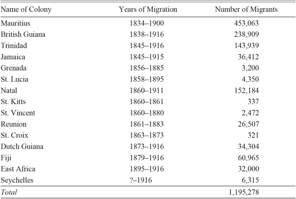
From 1838–1917, more than one million Indians eventually became indentured servants to a variety of locations. This is roughly 20 percent of the estimated population that travelled under various forms of contracts to outlying areas of British India and worldwide during this period (Northrup Reference Northrup2003). Mauritius was the first colony to experiment with importing Indian labor, and the practice spread to other British colonies. Natal and Fiji stand out as later primary destinations. Several French colonies, including Cayenne (French Guiana), Guadeloupe, Martinique, and Reunion, adopted indentureship, although many migrants departed not from British India but rather from French India. Dutch Guiana (Suriname) and the Danish island of St. Croix also petitioned British officials for indentured migrants and were permitted to do so, although the latter received only one ship and discontinued the practice within a decade. Officials in India required the Dutch to build a similar indentureship bureaucracy in Dutch Guiana as in British colonies, and British officials in Trinidad oversaw Danish indentureship. Table 1 gives an overview of the years of indentureship and the number of migrants to various destinations.

TABLE 1

ESTIMATED STATE-SPONSORED INDENTURED IMMIGRATION FROM INDIA

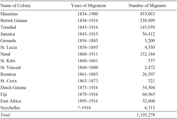
Source: Adapted from Lal (Reference Lal1980), Roopnarine (Reference Roopnarine2010). Lal (Reference Lal1980) is unable to fix the date at which immigration to the Seychelles began.

Contracts specified the length of time, usually five years; a fixed wage for the categories of men, women, and children; food, housing, and medical benefits; and the provision of additional benefits at the end of the contract. On arrival, workers were allocated to a particular estate and could not easily switch employers; most transfers came from purposes of family reunification. Remarkably, the contractual terms remained stable over long periods of time except for minor pay adjustments for new indentured laborers. As noted earlier, this contrasts sharply with the colonial American case with private, individualized contracts. Contracts did, however, vary across colonies. Like master-servant contracts in the United Kingdom proper, breach of the indentureship contract was a criminal, not civil, offense. This criminalized desertion and removed the option of moving between employers without prior approval.

Indians primarily worked in sugarcane and other agricultural commodities in the recipient destinations. Tasks included planting, hoeing and weeding, cutting, and working in sugar factories. Indentureship was designed to be temporary, and there were initially few structures to facilitate long-run migration. In contrast, many colonies put measures in place to discourage settlement, such as a poll tax in Natal and limited landownership rights in Fiji.

The growing home rule movement in India viewed indentureship negatively as an institution designed to exploit Indian labor for low wages. In Natal, Gandhi launched a strong political challenge against the imposition of a high poll tax on free, post-indenture Indians in the 1890s. The annual poll tax was set at £3 after being proposed at £25. In context, an indentured Indian earned just £6 per year. Gandhi and other local opponents pointed to segregation in Natal and the use of indentureship to restrict labor and economic mobility in the colony. After his return to India in the 1910s, Gandhi joined other nationalists to campaign against indentureship. In his autobiography, Gandhi points to the continuation of the poll tax in Natal and the second-class status of Indians generally as catalysts for his opposition to indentureship (Gandhi Reference Gandhi and Mahadev1927). The government in India halted indentureship in 1917 due to political pressure from Gandhi and others, and the last indentured immigrants completed their contracts in the early 1920s. Despite this, thousands of Indians continued to sign on as indentured laborers up until the government-imposed cessation.

Fiji, Jamaica, Natal, and Suriname form the primary focus of this article due to the preservation and digitization of their records. In Fiji and Natal, Indian labor was essential to starting the indigenous sugar industry. By the early twentieth century, indentured Indian laborers worked in coal mines in Natal, as well. Legal barriers to hiring ethnic Fijians led to demand for Indians, and this division lasts to the present. In Suriname, Indians replaced emancipated slaves in the sugarcane estates and were replaced themselves during and after WWI by Javanese indentured laborers.

MODEL OF MIGRATION CHOICE

Building from the canonical work from John Harris and Michael Todaro (Reference Harris and Michael1970) and George Borjas’s use of the Roy Model (Reference Borjas1987), I outline a migration model that includes uncertainty, risk aversion, and intertemporal decision making. The model highlights the long-run nature of indentureship and risk-mitigation, which previous models have omitted. This approach differs from John Kennan and James Walker (Reference Kennan and James2011) by placing uncertainty on the home side. The use of uncertainty and risk aversion poses different implications than the Harris–Todaro Model. In that model, expected wages in their urban sector depend on the probability of unemployment, and the equilibrium condition equalizes the unemployment-adjusted wage with the rural wage. Here, the equalization of expected consumption bundles across sectors does not lead to equilibrium; rather, the equalization of expected utility does. Although this point seems subtle, the underlying mechanism is different: Workers in my model face sending-market uncertainty and are risk averse, which in turn spurs migration.

Worker’s Problem

I use market 0 and market 1 as the home and recipient markets, respectively, to maintain consistency with Borjas. Laborers in market 0 live in J districts operating under a traditional economy subject to fluctuations in consumption prices. Initially, in a closed economy without migration, worker i’s utility in time t ∈ {1,2} and district j is given by U(c _ijt), where U is a concave function and c _ijt is consumption for person i in district j at time t.

The worker earns a real wage w _ijt = w _jt > 0 via subsistence production in each period. The distribution of wages is given by log(w _jt) = μ _j + ε _jt, where 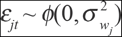$$ \varepsilon _{jt} \~\phi (0,\sigma _{w_j }^2 )$$. Workers live hand-to-mouth. The consumption good price is normalized to 1 within each district. The maximization problem immediately simplifies to c _ijt = w _ijt = w _jt. Note that $$\sigma _{w_j }^2 = \sigma _{c_j }^2 $$.

Now suppose that the worker can choose at the start of period 1 to migrate to a foreign labor market under a credible, guaranteed forward contract. The real wage of this contract is $$\widetilde w$$ and translates into $$\widetilde c$$ consumption, defined ex ante. By definition, $$\widetilde c$$ increases as $$\widetilde w$$ increases. Because the labor market is foreign, wages in the foreign market are independent of wages in any given village, that is, ∀j, . ⊥ $$\widetilde w$$_j. Assuming that the labor supply remains fixed across labor markets, the migration decision for i comes from the inequality,

(1) \begin{equation} \begin{array}{c}{(1+\beta) U\left(\tilde{c}_{J}\right) \leqq U\left(c_{j 1}\right)+\beta E\left[U\left(c_{j 2}\right)\right]} \\ {\underbrace{\beta^{-1}\left(U\left(\tilde{c}_{J}\right)-U\left(c_{j 1}\right)\right)+U\left(\tilde{c}_{J}\right)}_{\pi} \leqq E\left[U\left(c_{j 2}\right)\right]}\end{array} \end{equation}

where β < 1 is the discount factor. This resembles Douglas Massey et al.’s (Reference Massey, Joaquin and Graeme1993) basic formulation of returns but in discrete time with a guaranteed return over the worker’s earnings horizon. The worker observes the wage level in the village economy, $$\widetilde w$$ internalizes the monetary costs of migration, and there is no return migration due to the forward-looking nature of the foreign contract and the worker’s two-period lifespan.

This leads to several immediate implications. Higher wages in the foreign market raise the value of π and increase the probability of migrating, but higher wages in the origin market raise the current value of staying and reduce the probability of migrating. Importantly for this article, higher variation in home consumption, which captures uncertainty, lowers the expected utility of staying and increases the probability of migrating.

With σ _cj > 0, it is possible for local wages to exceed foreign ones and yet have migration. Intuitively, greater wage variation in the local market makes the certainty value of the foreign contract more appealing. I assume that agents form an expectation of σ _cj based on their past observations. This form of adaptive expectations means that higher fluctuations in consumption in a market j in the past imply further fluctuations in the future.

The upshot of the model seems to clash with Stephen Turnovsky, Haim Shalit, and Andrew Schmitz (Reference Turnovsky, Haim and Andrew1980) and earlier work on price volatility, in which price stabilization (or certainty) hurts consumers. However, price stability is beneficial in broad cases in which consumers spend large parts of their income on a good or risk aversion is high. Both of these conditions hold here: The worker consumes all of her income on the consumption good, and the worker is risk averse. Thus, the model’s predictions line up with earlier theoretical work on price variations.

This model distinguishes itself from Borjas’s use of the Roy Model in two major ways. First, the ex-ante wage contract collapses the foreign wage distribution to a single, predefined wage. I remove variation from one side of the migration decision. The skills, productivity shocks, and other factors in the home market that may lead to different wages are flattened. The correlation ρ _wj,w̃ between the wage at home and abroad becomes immaterial because the fixed w _f makes the value of migrating, π, known ex ante.

Second, the migration decision depends on an expectation of future income. The worker compares the foreign offer against the local distribution of wages and, based on a belief about the subsequent year’s wages, makes a decision. This lack of ex ante information about the origin market’s future, risk aversion, and incomplete consumption smoothing lead workers to migrate. In some cases, workers hedge their bets against volatility by migrating to avoid uncertainty.

Although this article focuses on workers, firms in the foreign market must be willing to hire laborers under forward contracts for migration to occur. I assume that the wage $$\widetilde w$$ offered under the contract is set exogenously (e.g., by law) and that laborers across markets are perfect substitutes. Workers are able to pursue an outside option that pays w _ft.

Several different reasons emerge why a firm in market 1 would want to hire labor under a forward contract. First, there could exist wage wedges between markets. Forward contracts create monopsony power and thus lower the arbitrage opportunities for immigrant workers. Firms earn more profits by undercutting laborers from their own market with laborers from market 0. Compensating differentials may play a role here if the work is onerous enough to raise local wages, w _ft. The statutory wage may not account for this, perhaps intentionally, and so w̃≪w _ft.

Second, firms could face problems with labor shortages. If the production function is more labor intensive for some fraction θ of the total production time, then labor rationing may occur during θ. This is true for many agricultural products, including sugar cane, due to a narrow window for harvesting. This creates a hold-up problem for employers in which laborers can attempt to extract higher wages during θ. With mobile labor, some firms could lose actual production while other firms could produce but at the cost of paying out higher spot wages. Following Evsey Domar (Reference Domar1970), the use of bonded labor—here, laborers under forward contracts— bypasses labor shortages during critical production periods. For firms, this is analogous to implicit wage contracts with non-existent labor mobility. Here, the institutional constraint on mobility due to indentureship makes the contract acceptable to firms and gives them positive profits.Footnote ¹

Third, forward contracts to capture the gains of specific human capital may exist if L = g(L,H) where H is human capital gained through on-thejob experience or training. With forward contracts, the same firm would bear any training cost (or lower production during training) in return for the higher gains in the future.

DATA ON INDENTURED SERVANTS AND LOCAL PRICES

The existence of demand for indentured servants working under forward contracts is apparent in the more than one million indentured servants shown in Table 1. Therefore, I turn to the labor supply side. I focus on Fiji, Jamaica, Natal, and Suriname to provide extensive coverage of source districts in India and destinations abroad. I utilize data from several sources to construct Indian district-level panel data, the most disaggregated level at which price data exist from India.

No single source provides counts of outflows by district either to specific colonies or overall. Some aggregated information appears for selected districts in the Annual Report of the Protector of Emigrants, quoted in Sarup (2006–2012). However, these data are not comprehensive and only cover departures from Calcutta. To solve this problem, I turn to the original, individual-level data to create district-year flows. As far as I am aware, I am the first scholar to create such measurements of district out-flows to foreign colonies.

The individual emigration pass, which was issued to all migrants on departure from India, forms the backbone of my data. The pass recorded information such as name, father’s name, caste, age, and place of origin. Due to the bureaucratic nature of the passes, which were created to identify indentured servants both in India and in the destination colony, the data are presumed to accurately represent the population. On the one hand, administrators received no benefit from falsifying records in India. Poor identification of a person could hinder the enforcement of the contract, which was adjudicated in criminal court. On the other hand, while the immigrants could manipulate some of their responses, the passes were used to assist with sending remittances, future repatriation, and locating relatives for estate bequests in case of death. Overall, therefore, the data should accurately represent the population leaving India.

I assembled individual-level data from several sources (Persaud Reference Persaud2019). I digitized all 60,000-plus emigrations passes for Fiji held by the National Library of Australia. I also digitized data from the last 12 years of Jamaica’s indentureship based on 5,000-plus original records held by the National Archives of Jamaica. I obtained various data for Natal (ca 150,000 records) and Suriname (ca 30,000 records) from the University of KwaZulu-Natal and the Dutch National Archives, respectively. I subsequently collapsed outflows to the district-year level. Per the Statistical Abstract Relating to British India (various years), I covered almost 40 percent of all Indians leaving as indentured servants in my study period. Roughly 30 percent of the population I gathered was female and the average age for an adult was in the early 20s. These two pieces of information matched what Lal (Reference Lal1980, pp. 281–83) wrote about the population of indentured servants.

Although I observe all immigrants to a particular colony (or all immigrants within a period of time for Jamaica), I only observe the characteristics of immigrants and not of all people in a given district. That is, the micro-level data set consists of individuals who selected into migration, and this information is aggregated to the district-year level to generate a flow measure. Because I do not observe migration to all colonies with the microdata, I digitized district-year totals of indentured immigrants for available districts from various Annual Report of the Protector of Emigrants from Calcutta to compare against my numbers. These are effectively restricted to a handful of districts in north India due to record collection. I have not been able to find comparable data for migration from Madras, and state-level reports do not give information on district-specific flows.

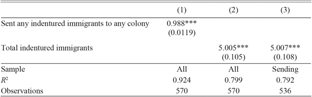
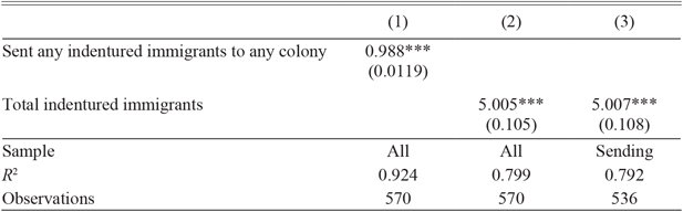
For Bihar and the United Provinces, I have reconstructed approximate totals for main districts prior to 1904. Unfortunately, it is not possible to use the aggregated data from reports in lieu of the microdata due to inconsistencies in the aggregated data. Appendix Table A1 shows that my microdata represent the total population well. Simple cross-tabulations show that more than 90 percent of districts are correctly identified as either sending or non-sending districts. In regressions of both a binary indicator for any migrants and the total migrants listed in the reports, my respective measures perform well with r Footnote ² values of roughly 0.9 and 0.8, respectively.

APPENDIX TABLE A1

CHECK AGAINST ANNUAL REPORTS (UP/BIHAR)

Notes: Dependent variable: Indentured servant outflows by district to any overseas colony calculated from annual reports, 1873–1903. Independent variable: Author’s calculation of outflows by district to Fiji, Jamaica, Natal, and Suriname. Standard errors in parentheses. Only districts in the United Provinces and Bihar are included. All models drop the constant. * p < 0.1, ** p < 0.05, *** p < 0.01.

Source: Indentured servant outflows any overseas colony calculated from annual reports and reported by Sarup (2006–2012) from 1873–1903. District-level outflows calculated by the author for Fiji, Jamaica, Natal, and Suriname, 1873-1916.

An immigrant’s district of origin links her to district-level prices. I focus on rice prices to have a consistent commodity across districts. Unlike other crops, rice is reported for almost every district-year pair. The annual, within-district correlations in the study period between rice and bajra, jowar, ragi, and wheat are 0.74, 0.72, 0.84, and 0.7, respectively. The correlation between rice and wheat, the second most important crop, rises to 0.77 when limiting the sample to the core wheat areas of Central India, the Central Provinces, Punjab and the NWF Province, Rajputana, Sind and Baluchistan, and the United Provinces. Additionally, given rice’s wide geographic scope and trade across South Asia, local, non-rice crops’ prices may fluctuate more than rice. John Hurd (Reference Hurd1975) and Dave Donaldson (Reference Donaldson2018) find that railroad construction led to price convergence of traded commodities during the same time period as indentureship. Given that rice was a major commodity even outside of rice-growing areas, this likely biases me against finding a result for rice price volatility.

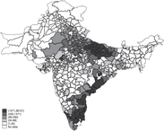
For the main analysis in the next section, I rely on districts that have rice price information and that ever sent one migrant. This reduces the problem of differing institutional environments and distances from ports that could differentiate districts that did send migrants from those that did not. Figure 1 shows the geographic distribution of districts that ever sent indentured immigrants to Fiji, Jamaica, Natal, or Suriname. This restriction affects marginal areas in Bengal and Assam in the northeast towards Burma; parts of western and northwestern India; tribal and sparsely populated jungle areas in modern-day Jharkhand and Odisha; and parts of central Deccan. These provinces were far away from the main ports and were often inaccessible (Sharma Reference Sharma2011). The main sending areas were in the northern Indo-Gangetic plain and along the coast in the south. I also exclude years in which immigration was suspended by law, since a zero in such years differs from a zero in years during which immigration was allowed. This removes two years: 1917, the last year of indentureship in which none of the four colonies I study recruited that late, and 1899 in the Madras recruitment area, which faced a plague outbreak.

FIGURE 1

DISTRICTS OF ORIGIN OF INDENTURED IMMIGRANTS TO FIJI, JAMAICA, NATAL, OR SURINAME, 1873–1916

Source: Author’s calculation from original records.

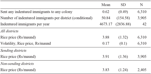
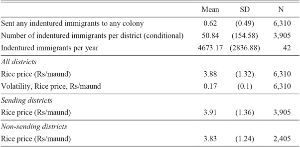
Table 2 gives summary statistics of the key district-level variables. Roughly two-thirds of the district-year observations send at least one indentured migrant. Some districts, such as Basti, sent a migrant in every year; on the other hand, Simla and others only sent migrants in one year. Arcot in the Madras Presidency sent so many migrants that arkaati entered Hindi as a term for an indentureship recruiter (McGregor Reference McGregor1993). Conditional on sending at least one migrant in a year, a district sent on average 51 migrants. On average, more than 4,800 new indentured servants left India each year for one of these four colonies. Rice prices averaged 3.88 Rs/maund, a measure of roughly 37 kilograms. I split the sample to show annual prices for “sending” and “non-sending” districts-year observations (where “sending” means there was at least one migrant). Rice prices are slightly higher in district-years that do not send migrants than in those that do. The standard deviation of rice prices for sending districts exceeds that of non-sending districts.

TABLE 2

DISTRICT-LEVEL DATA SUMMARY STATISTICS

Source: District-level outflows calculated by the author for Fiji, Jamaica, Natal, and Suriname, 1873–1916. Prices calculated from Prices and Wages in India. Volatility is the standard deviation of the change of log(rice prices) over the past five years.

The focus on prices rather than wages stems from systematic problems with existing wage data. The method of collecting wages was revised in the early 1900s, whereas prices were collected consistently from 1862 onwards (Prices and Wages in India 1921, p. 2). Wages prior to 1900 were collected in fewer districts than prices and in a coarser fashion. For example, a wage might be designated as “2 to 4 rupees.” Wages or wage ranges are often sticky across an area or time (e.g., wages in a province may all be the same or the wages for a district may be the same for many consecutive years), which Gupta and Swamy (Reference Chaudhary and Anand2017) also note. While nominal wages could have moved in the earlier example between two and four rupees, the reported wage may not have changed. The magnitude of the wage differential between districts in India and colonies should be approximately correct, but the exact differential (and volatility) may be incorrect. Without more information or stronger assumptions on the distribution of wages within a range over time, real wages cannot be precisely calculated.

British colonial officials also expressed their belief that staples’ price changes, rather than a fall in wages, explained changes in well-being because of the minimal responsiveness of wages to changing conditions (e.g., District Gazetteers of the United Provinces of Agra and Oudh 1904). Wages could have been set more by custom and, in the presence of surplus labor, have been difficult to adjust. Prices, on the other hand, could adjust more easily and clear the markets vis-à-vis a stickier wage.Footnote ²

I define a volatility variable similar to prior literature in finance and trade (e.g., Tenreyro Reference Tenreyro2007). Volatility for district j in year t is the standard deviation of the first difference of the logarithm of annualized prices p over the past m periods:

(2) $$ \matrix{ {z_{j,t,m} = \ln {\rm{ }}p_{j,t - m + 1} - p_{j,t - m} } \hfill \cr {\nu _{jt} = SD[z_{j,t,m} ],m = 1{\rm{ }}...{\rm{ }}5.} \hfill \cr } $$

I use five years (m = 5) to match the contract length in the recipient colony. The measure is defined within each district.

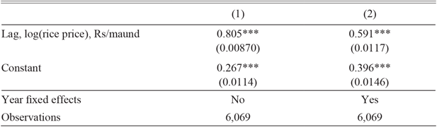
The functional form of volatility relies on a view of adaptive expectations in which past realizations of price and volatility affect the expectation of the future outcome. To justify this, I run autoregressive models of log rice price with one lag using my dynamic panel. Despite having more than 40 years of data, consistency may be an issue with a static model because prices show autocorrelation. The equations are a simple autoregressive process:

(3) $$ y_{jt} = \rho y_{j,t - 1} + \gamma _j + \delta _t + \varepsilon _{jt} ,$$

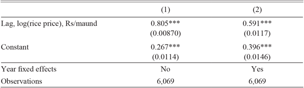
where j indexes the district, t indexes time, and y is the log of rice price. I take the first difference in order to use the Arellano–Bond (Reference Arellano and Stephen1991) GMM estimator. Appendix Table A2 shows the results with and without δ _t. For both equations of interest, ρ is positive, significantly higher than 0, and significantly lower than 1, which implies stationarity and autocorrelation. Without time fixed effects, the value of ρ is above 0.8, though this drops to just below 0.6 with fixed effects. Overall, this shows that past price realizations could be used correctly as part of a forecasting model.

APPENDIX TABLE A2

DYNAMIC PANEL CHECK

Notes: Dependent variable: Log of rice price. Standard errors calculated by GMM in parentheses. Both models include exactly one lag of log rice price in a dynamic panel (Arellano–Bond) model. * p < 0.1, ** p < 0.05, *** p < 0.01.

Source: Prices calculated from Prices and Wages in India.

To reflect the pull forces from the overseas destinations, I entered contract information provided by various years of the Annual Report of the Protector of Emigrants in Calcutta. The Protector of Emigrants in Calcutta, the chief official who oversaw overseas emigration, created these reports based on information from India and the recipient colonies. The reports include standardized tables outlining the contracts. Wages in Fiji, Jamaica, and Suriname were set at one shilling per diem during the entire period. Wages in Natal were set at 10 shillings per month. However, Natal’s contracts stipulated complete provision of food for the duration of the contract, while the other colonies provided food for a specified period of time and price.

To generate my measure of colonial wages, I use the rupee-sterling exchange rate given by Raymond Goldsmith (Reference Goldsmith1983) and the colonial wage defined by law less food at government-set prices. All colonies initially deducted money for food, and there is evidence that government-set food prices were inflated (Knapman Reference Knapman1985). Take-home wages rose once colonies stopped food deductions. Wages in the colonies rose to their highest (in rupee terms) at the end of the nineteenth century and then flattened once the silver-denominated rupee was pegged to the gold standard.

FINDINGS

With the assembly of a district-level panel of outflows (aggregate and by colony), rice prices, rice price volatility, and overseas wages, I can answer the primary question: Does higher rice price volatility correlate with higher out-migration under indentureship? Next, to check for heterogeneous effects based on differing overseas contracts, I separate the effect by colony. Finally, to capture the effect of chain migration, I estimate the same impact while accounting for prior outflows.

District-Level Indentured Migrant Flows

The first outcome of interest is the sending of any migrant from a district j, that is, the role of volatility on the extensive margin. Given the wide coverage of recruiters, each district can be seen as possessing the opportunity to send a migrant. Table 2 also shows that many districts complied. I first estimate a linear probability model with fixed effects to test whether rice price volatility is associated with the probability of a district sending any migrants in a given year. The estimating equation is

(4) $$ any_{jt\,} = \beta _0 + \beta _1 {\rm{ ln(}}MinColonyWage_t {\rm{)}} + \beta _2 {\rm{ ln(}}price_{jt} {\rm{) }} + \beta _3 \nu _{jt} + \Gamma I_j + \varepsilon _{jt} , $$

where j indexes a district, t indexes year, and v _jt is the measure of rice price volatility in a given district-year (as described earlier). I use the minimum wage (net of food) offered across the four recipient colonies to get a conservative bound on the pull factor of wages. The district fixed effect captures the amenity value of a district and other fixed unobservables.

As noted earlier, I focus primarily on rice prices to ensure a comparable food unit across India. $$\mathord{\buildrel{\lower3pt\hbox{$\scriptscriptstyle\frown$}}\over \beta } _3 $$ is the key coefficient of interest as part of the risk-aversion/consumption-smoothing story because it captures the within-district effect of volatility. Traditional migration models predict a positive, significant coefficient on recipient-colony wages, that is, a wage-differential story.

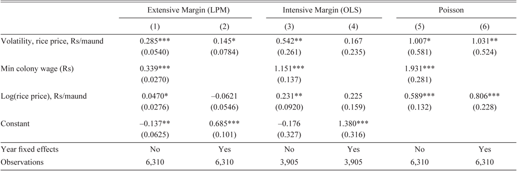
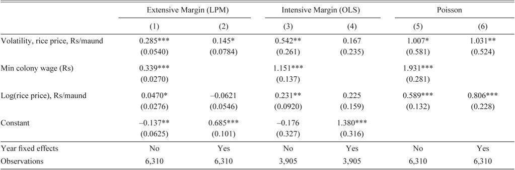
The first two columns in Table 3 show regressions based on Equation (4). Column 1 includes the volatility measure, and $$\mathord{\buildrel{\lower3pt\hbox{$\scriptscriptstyle\frown$}}\over \beta } _3 $$ is positive and statistically significant at the 1 percent level. This is consistent with risk aversion and consumption smoothing: Higher levels of price volatility induce more uncertainty, which in turn raises the probability of migration. A rise of volatility by one-standard deviation raises the probability of migration occurring from that district by almost 3 percentage points relative to a mean of 62 percent.

TABLE 3

MIGRATION WITH RICE PRICES

Notes: Columns 1–2 dependent variable: Sent any indentured immigrants to any colony. Columns 3–4 dependent variable: Log total indentured immigrants to any colony. Columns 5–6 dependent variable: Total indentured immigrants to any colony. Bootstrapped standard errors clustered by district in parentheses. All models include district fixed effects. * p < 0.1, ** p < 0.05, *** p < 0.01. Volatility is the standard deviation of the change of log(rice prices) over the past five years.

Source: District-level outflows calculated by the author for Fiji, Jamaica, Natal, and Suriname, 1873–1916. Prices calculated from Prices and Wages in India.

I add year fixed effects in the second column and drop the minimum colony wage because it varies at the year, but not district-year-level. Column 2 is the main column of interest: The coefficient on volatility drops in significance to the 10 percent level and also falls in magnitude, but higher volatility is still positively associated with a district sending at least one indentured servant. A rise in volatility of one-standard deviation raises the probability of a district sending a migrant by 1.45 percentage points. These columns illustrate the main result: external wages pulled Indians out, and internal price volatility pushed people out.Footnote ³

Prices, wages, and volatility may have affected migration not only on the extensive margin but also on the intensive margin. Thus, the number of total indentured servants who chose to migrate is also an outcome of interest. To address this, I modify the previous equation by using the log of indentured immigrants in each district-year as the dependent variable. The analogue to Equation (4) is

(5) $$ \ln (Indenture_{jt} ) = \beta _0 + \beta _1 {\rm{ ln(}}MinColonyWage_t {\rm{)}} + \beta _2 {\rm{ ln(}}price_{jt} {\rm{) }} + \beta _3 \nu _{jt} + \Gamma I_j + \varepsilon _{jt} . $$

Table 3, Columns 3 and 4 remove districts that did not send any migrants in a given year and focuses instead on the intensive effects.

The coefficient on volatility is positive and statistically significant at the 5 percent level in Column 3. A one-standard deviation increase in volatility is associated with a five-percent increase in the number of indentured immigrants. Volatility is still positive but smaller and not statistically significant in Column 4 when time fixed effects are added. The coefficient on the log of rice price is positive and significant at the 1 percent level in Column 3 and at the 5 percent level in Column 4. The magnitude is similar across all specifications: a 10 percent rise in rice prices raises the number of indentured servants by roughly 2 percent. Recipient-colony wages are positive and significant at the 1 percent level in both Columns 1 and 2. A rise in wages raises the number of indentured migrants roughly by the same proportion.

To analyze the two dependent variables together and check if the results still hold given the drop in significance from extensive- to intensive-margin regressions, I run Poisson regressions on the counts of indentured servants. The equation is of the form

(6) $$ \matrix{ {{\rm{E}}[Indenture_{jt} {\rm{ }}|{\rm{ }}X_{jt} ]{\rm{ }} = {\rm{ }}\exp [\theta _1 ,{\rm{ }}\theta _2 ,{\rm{ }}\theta _3 ;{\rm{ }}\Theta _4 ]\& \# x2032;} \hfill \cr {[\ln (MinColonyWage_t ,{\rm{ }}\ln (price_{jt} ),{\rm{ }}v_{jt} ;{\rm{ }}I_j ],} \hfill \cr } $$

where the second vector contains the same covariates as mentioned previously: log of the minimum recipient-colony wage, log rice price, log wage, rice price volatility, and district fixed effects.

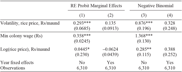
Table 3, Columns 5 and 6 show the results from this regression. The signs of the coefficients match the theoretical expectation in all columns. Although volatility is only significant at the 10 percent level in Column 5, it is significant at the 5 percent level in Column 6. In both columns, a one-standard deviation increase in rice price volatility raises the log of the expected count of migrants by 1. Recipient-colony wage is significant in Columns 1 and 2 at the 1 percent level. Log rice price is significant at the 1 percent level in all columns. This strengthens the evidence from the previous tables that volatility matters in out-migration under indentureship contracts.

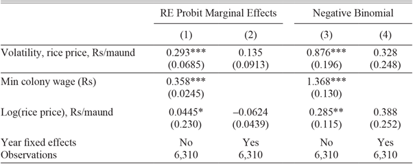
As a robustness check due to a high number of zeros in the data and to deal with potential misspecification therefrom, I run negative binomial regressions of the same form as the Poisson regressions. Appendix Table A3, Columns 3 and 4 show these results. Volatility is positive and significant in Column 3 (without year fixed effects), but it is no longer significant in Column 4 (with year fixed effects). However, this is largely consistent with the Poisson results.

APPENDIX TABLE A3

MIGRATION WITH RICE PRICES, ROBUSTNESS CHECKS

Notes: Columns 1–2 dependent variable: Sent any indentured immigrants to any colony. Columns 3–4 dependent variable: Total indentured immigrants to any colony. Bootstrapped standard errors in parentheses. All models include district fixed effects. * p < 0.1, ** p < 0.05, *** p < 0.01. Volatility is the standard deviation of the change of log(rice prices) over the past five years.

Source: District-level outflows calculated by the author for Fiji, Jamaica, Natal, and Suriname, 1873–1916. Prices calculated from Prices and Wages in India. Contractual wages calculated from original contracts or annual reports and cross-checked with Sarup (2006–2012).

Overall, volatility emerges as significant for both the extensive and intensive margins. The covariates are signed correctly according to theory. They consistently show that higher-volatility districts were more likely to send indentured servants and, conditional on this, likely to send more. The relationship does appear more robust for the extensive margin, which may indicate the importance of a threshold model of leaving or the importance of linked migration, which I explore later.

Robustness: Cross-Colony Differences

The models noted earlier pool all the colonies together, but contract variations could lead to different patterns of migration across colonies. In particular, the contracts for Natal paid lower wages than the other colonies but included food for the entire duration of the contract. The completely guaranteed nature of Natal’s contracts suggests that migration to Natal might be highly responsive to origin-market volatility.

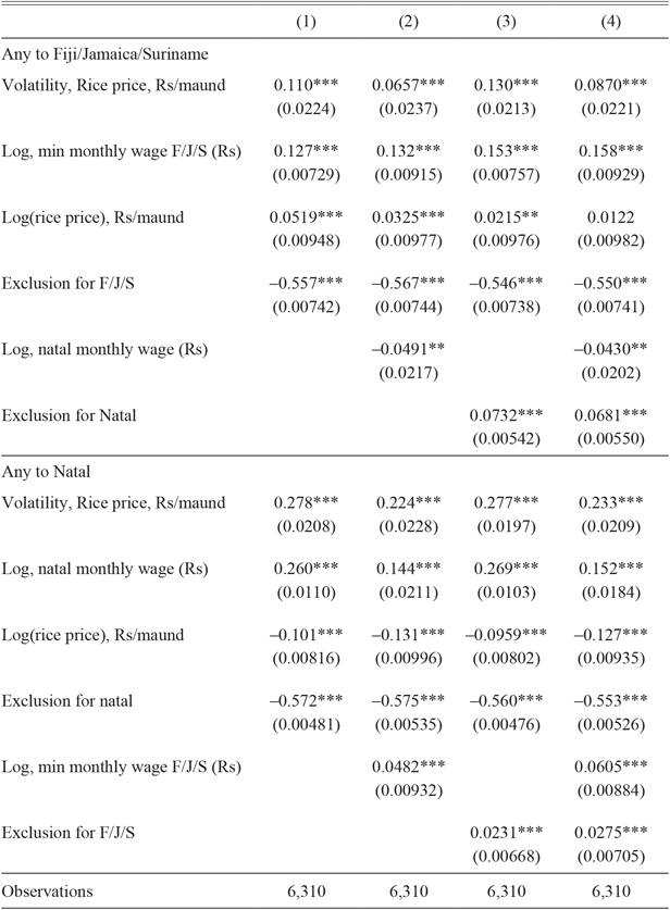
To examine colony-specific migration patterns, I compare Natal to the other three colonies, which resembled one another in wages and terms for other fringe benefits. I run panel seemingly unrelated regressions (SUR) on the binary variable that indicates whether district j sent at least one indentured servant to colony c, where c is either (1) Natal or (2) the pooling of Fiji, Jamaica, and Suriname. The model stacks equations from the two groups of the form

(7) $$ any_{jct} = \beta _0 + \beta _1 {\rm{ ln(}}wage_{ct} {\rm{)}} + \beta _2 {\rm{ ln(}}price_{jt} {\rm{)}} + \beta _3 \nu _{jt} + \beta _4 exclusion_{jct} + \Gamma I_j + \varepsilon _{jct} , $$

where c indexes the colony, j the district, and t the year. The error terms are allowed to be correlated across c. Dropping a colony-district-year observation leads to dropping the entire district-year observation, so I include an extra dummy variable exclusion _jct that indicates that a colony c was excluded from indentureship recruiting in district j during a given year t. This is to ensure that the matrix of stacked outcomes is defined across all districts for a given year. I do not run models with a year fixed effect due to computational problems with invertibility.

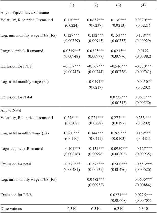
Table 4 gives the results from the SUR models. Across all specifications for both the pooled colonies and for Natal, volatility and own wage are significant at the 1 percent level. This mirrors the results from Table 3. The magnitudes in that table are more similar to those for Natal; this is unsurprising given that indentureship to Natal comprises about 60 percent of the underlying population of interest here.

TABLE 4

SUR WITH COLONY-SPECIFIC MIGRATION

Notes: Dependent variable: Sent any indentured immigrants. Destinations for seemingly unrelated regressions split into Natal vs. Fiji, Jamaica, or Suriname. Standard errors in parentheses. All models include district fixed effects. * p < 0.1, ** p < 0.05, *** p < 0.01. Volatility is the standard deviation of the change of log(rice prices) over the past five years.

Source: District-level outflows calculated by the author for Fiji, Jamaica, Natal, and Suriname, 1873–1916. Prices calculated from Prices and Wages in India.

In Column 1, I run Equation (7) as given. Again, in both panels, volatility and the pull wages overseas are positive and significant at the 1 percent level. Natal shows the larger magnitudes on its covariates, but in both panels, the coefficients on volatility and wage are similar. Columns 2 and 3 give some insight into the interactions of recruitment for different colonies. In the upper panel, the coefficient on volatility drops by roughly half once I account for Natal’s wages in Column 2. Higher wages in Natal are also correlated with lower indentureship to the other colonies. In contrast, the coefficient on volatility in the lower panel for Natal changes only slightly. In Column 3, the coefficients for exclusion in the other colony (e.g., covering the period after Natal suspended indentureship) is positive and significant at the 1 percent level in each panel. The volatility coefficients resemble the coefficients in Column 1. Column 4 is equivalent to two separate ordinary least squares (OLS) regressions, since the covariates do not vary between models, and mostly resembles Column 2.

Comparing migration across colonies reinforces the overall indentureship story but adds nuance to the individual colonies that accords with their contracts. Natal offered the most assured future for Indians, whereas the other colonies gave contracts that did not guarantee food for the entire time. In accordance with this, the coefficient on volatility is both larger in magnitude and roughly constant in the lower panel. The coefficient on Natal wages in the lower panel drops almost in half in Columns 2 and 4, which include wages in the other colonies. The reverse pattern emerges for the pooled group of Fiji, Jamaica, and Suriname in the upper panel: there is a more consistent coefficient on own wages across all columns and a fall in the volatility coefficient in Columns 2 and 4. Volatility mattered for recruitment to all colonies, but the inter-colony differences show that it mattered more for the most guaranteed colony, Natal.

Robustness: Accounting for Past Migration

Past out-migration from a district under indentureship could have affected subsequent take-up of indentureship contracts. Indentured Indians sent and received thousands of letters throughout the decades of indentureship, and many returned to India at the end of their contracts. Because I do not have data on other colonies that started earlier, particularly British Guiana and Mauritius, I do not instrument for subsequent out-migration under indentureship from the earliest possible outflows (e.g., in the 1840s and 1850s) or for an interaction of initial outflows with a time trend. Instead, I use the Arellano–Bond dynamic panel estimator with lags of the dependent variable as predictors for outflows. I choose five lags to match the volatility measure and the scope of the contracts. Because recent flows may also have been more salient than earlier ones, this also captures a potentially time-varying effect on subsequent migration.Footnote ⁴

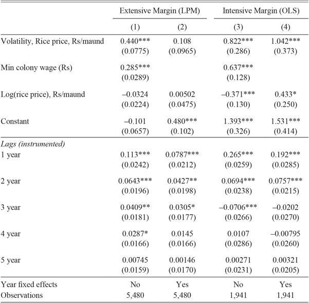
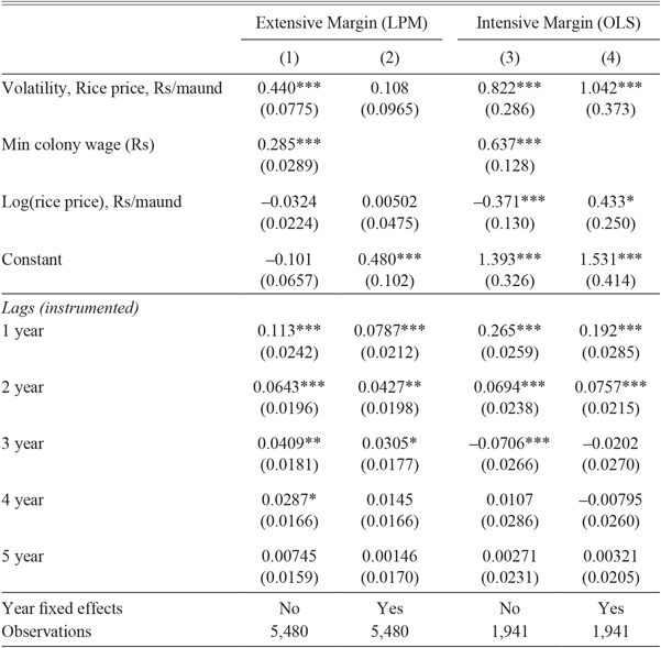
The extensive-margin Arellano–Bond results appear in Table 5, Columns 1 and 2. The sample size drops because the first few years lack sufficient lagged periods. Unsurprisingly, the coefficients on the lagged dependent variables for one through three years prior are positive and statistically significant in both columns. The one-year lag has the highest coefficient, and the coefficients on the lagged instruments drop monotonically further back in time. This is consistent with fast information-sharing and recruitment patterns that may extend across calendar years in a given district. The drop in magnitude and significance over time shows the effect weakens.

TABLE 5

MIGRATION WITH RICE PRICES AND LAGGED MIGRATION

Notes: Columns 1–2 dependent variable: Sent any indentured immigrants to any colony. Columns 3–4 dependent variable: log total indentured immigrants to any colony. Standard errors calculated by GMM in parentheses. All four models cover 1873–1916 and include exactly five instrumented lags of log rice price in a dynamic panel (Arellano–Bond) model as described in the text. Volatility is the standard deviation of the change of log(rice prices) over the past five years.

Source: District-level outflows calculated by the author for Fiji, Jamaica, Natal, and Suriname, 1873–1916. Prices calculated from Prices and Wages in India. Contractual wages calculated from original contracts or annual reports and cross-checked with Sarup (2006–2012).

The results for volatility and overseas colony wages resemble the main specification in Table 3. Volatility is positive and statistically significant at the 1 percent level in Column 1 (without fixed effects) and positive but not statistically significant in the second column. The magnitude rises slightly but is not significantly larger than the earlier, base model. Even after controlling for the network or chain migration effect, volatility still is correlated with out-migration on the extensive margin.

The analogous intensive-margin estimates appear in Table 5, Columns 3 and 4, and reaffirm the main findings from Table 3, Columns 3 and 4. The stronger effect of the prior year on out-migration appears with larger coefficients on the one-year lag than any other year. The three-year lags show a negative sign in the first two columns, but they are indistinguishable from zero once year fixed effects are included.

The key finding from this table is that volatility remains positive and significant at the 1 percent level even when accounting for lagged flows in Columns 1 and 3 and controlling for year fixed effects in Column 4. The magnitudes are larger than those in Table 3, which lacks the lags. In Column 2, the relative magnitude of the overseas wage is lower than that of volatility, although the standard errors are larger for volatility and the two are not statistically different.

Overall, networks may play a role in indentured migration but the effect rapidly diminishes. Furthermore, networks do not fully explain the dynamics of out-migration under indentureship or remove the evidence for volatility. The magnitudes of the correlations between volatility and out-migration, both extensive and intensive, remain similar to the original specifications. Volatility still plays a role in understanding out-migration under indentureship contracts.

CONCLUSION

This article provides new evidence on an understudied topic: South-South migration during the “Age of Migration.” I find that volatile economic outcomes in India were an important determinant of migration, particularly when a forward contract was available to reduce the negative impacts of these fluctuations. The importance of volatility to migration decisions is consistent with basic economic theory: risk-averse agents prefer consumption smoothing. Given India’s poverty and fluctuating economic conditions, this may provide insight into why migration under informal bonded labor systems, such as kangani and maistry, occurred rather than self-funded, individual, free migration (Jain Reference Jain, John, Anthony and Rutledge2015). Indian indentureship may also offer lessons for studying other contemporaneous South-South migrations, such as Chinese and Javanese forms of indentureship

The dearth of other studies on volatility makes it difficult to benchmark my results, but Robin Burgess and Dave Donaldson (Reference Burgess and Dave2012) examine the impact of railroad expansion on commodity prices in India. They find a decline in the coefficient of variation of district-level commodity prices to be 75 percent over a much longer span of time (1870–1930). While coefficient of variation does not equal my measure of volatility, a 75 percent drop in volatility implies a drop in the likelihood of a district sending an indentured immigrant of 1.8–3.6 percent. This compares favorably to a 1.5–3 percent change in the likelihood of sending an indentured immigrant from a one-standard deviation change in volatility. The secular decline of commodity prices does not remove the likelihood of a district sending any indentured immigrants.

The institutional context of Indian indentureship reduced uncertainty on one side of the migration decision and allows me to study how local prices, price volatility, and foreign wages influenced migration. As seen, higher rice price volatility was associated with both the presence of indentured servants from a district and more indentured servants. My colony-specific results provide evidence that more volatile areas sent more indentured servants to Natal, which is also consistent with theory given Natal’s greater contractual guarantees. Social networks, as proxied by lagged migration, contributed to migration flows, but even still, higher volatility was associated with higher out-migration from India.