





1. Introduction
The sedimentation of particles in a viscous fluid is a classical problem in fluid mechanics, and plays an important role in many industrial and natural processes. For example, the fate of microplastics found on the seabed is a prominent environmental question, which requires predictions of particle transport, deposition and resuspension (Claessens et al. Reference Claessens, Van Cauwenberghe, Vandegehuchte and Janssen2013; Turner Reference Turner2021). In many applications the flow induced by sedimenting particles is inertially dominated and much of the particles’ complex behaviour is due to the associated nonlinear effects (see e.g. Ern et al. (Reference Ern, Risso, Fabre and Magnaudet2012) and Heisinger, Newton & Kanso (Reference Heisinger, Newton and Kanso2014) for an overview of different behaviours exhibited by planar disks sedimenting at finite Reynolds number). However, handling and processing of microscale materials, such as ultrathin graphene flakes and other colloidal objects in liquid environments typically involves flows at small Reynolds number (Khan et al. Reference Khan, O'Neill, Porwal, May, Nawaz and Coleman2012; Ma et al. Reference Ma, Cui, Du, Xu, Deng and Zhu2021; Silmore, Strano & Swan Reference Silmore, Strano and Swan2021). In the same inertialess regime, single particle sedimentation has been utilised for understanding the size-separation of DNA and other biological proteins (Weber et al. Reference Weber, Carlen, Dietler, Rawdon and Stasiak2013), and improving clinical blood tests (Peltomäki & Gompper Reference Peltomäki and Gompper2013).
In the Stokes limit of vanishing inertia, the sedimenting particle's shape is the key factor determining its motion, and the behaviour of many simple objects in unbounded fluids is well understood. For instance, at zero Reynolds number spheres sediment purely vertically (Stokes Reference Stokes1851), while straight rods and flat circular disks sediment with a constant horizontal drift and without changing their orientation (Brenner Reference Brenner1963). Conversely, chiral particles (such as a propeller-shaped objects) continually reorient while sedimenting, resulting in spiral trajectories (Doi & Makino Reference Doi and Makino2005; Witten & Diamant Reference Witten and Diamant2020). The sense of rotation of such screw-like objects is determined by their geometry (see Gonzalez, Graf & Maddocks (Reference Gonzalez, Graf and Maddocks2004) for a comprehensive analysis). However, despite the existence of a well-established theoretical framework, which uses the mobility or resistance matrix to link the particle's translational velocity and its rate of rotation to the forces and torques acting on it (Happel & Brenner Reference Happel and Brenner1983), predicting the qualitative behaviour of an arbitrarily shaped sedimenting particle in an infinite fluid at zero Reynolds is still an open question (Collins et al. Reference Collins, Hamati, Candelier, Gustavsson, Mehlig and Voth2021; Huseby et al. Reference Huseby, Gissinger, Candelier, Pujara, Verhille, Mehlig and Voth2024).
The behaviour of individual particles has an important effect on their collective behaviour in dilute suspensions, i.e. in a regime when interactions between particles can be neglected. For instance, a dilute cloud of spheres will sediment without changing its shape while dilute clouds of straight rods or planar disks will disperse because each individual particle will move in a different direction and with a different speed, depending on the particles’ random initial orientations. To the best of our knowledge, all chiral objects investigated so far sediment with non-zero horizontal velocities, but their spiral trajectories imply that, on average, they sediment purely vertically (Witten & Diamant Reference Witten and Diamant2020; Huseby et al. Reference Huseby, Gissinger, Candelier, Pujara, Verhille, Mehlig and Voth2024). This implies that a dilute cloud of such objects sediment with net zero horizontal dispersion.
If the sedimenting particles are sufficiently flexible, the deformation induced by the fluid traction can change their behaviour. For instance, sedimenting elastic fibres tend to deform into a U-shape and then right themselves until they reach an upright-U orientation, following which they sediment steadily without any horizontal drift – unlike their rigid counterparts. The sedimentation of such flexible fibres has been studied extensively (see, e.g. Li et al. Reference Li, Manikantan, Saintillan and Spagnolie2013; Marchetti et al. Reference Marchetti, Raspa, Lindner, du Roure, Bergougnoux, Guazzelli and Duprat2018), but there is far less work on the effect of fluid–structure interaction on the sedimentation of other objects. Recent experiments of Miara (Reference Miara2024) and numerical situations of Yu & Graham (Reference Yu and Graham2024), showed that sedimenting flexible sheets can also deform into a U-shape, similar to the shape adopted by sedimenting fibres.
Motivated by these observations, Miara et al. (Reference Miara, Vaquero-Stainer, Pihler-Puzović, Heil and Juel2024) performed an experimental study of the sedimentation of such objects, focusing on the behaviour of rigid U-shaped disks which we created by the isometric deformation of a circular disk onto the surface of a circular cylinder, as shown in figure 1(a). The resulting U-shaped disk has two planes of symmetry and, crucially, is non-chiral. We studied the sedimentation of such disks in a viscous fluid, with the viscosity and density difference chosen such that the resulting flow had a small Reynolds number. Our experiments showed that over the experimentally observable length scales (limited by the size of the tank in which the experiments were performed), such disks never settled into a steady motion but continued to reorient, with concomitant continuous changes to their velocity. A careful analysis of the observed trajectories showed that this behaviour is due to the disks undergoing a periodic sequence of rolling and pitching motions (see figure 1b–e for an illustration of the terminology and the angles used to describe the disk's orientation) which resulted in a sedimentation along complicated spiral trajectories whose chirality is determined by the disk's initial orientation, rather than being set by the (non-chiral) particle shape (Miara et al. Reference Miara, Vaquero-Stainer, Pihler-Puzović, Heil and Juel2024).
(a) Schematic of the isometric deformation of a flat circular disk onto the surface of a cylinder of radius  $R_c$. (b–e) Tait–Bryan angle convention following the intrinsic
 ${\rm yaw}\rightarrow {\rm pitch}\rightarrow {\rm roll}$ sequence, showing (b) the reference frame
 $\mathcal {F}_0$, (c,d) the orientation in the intermediate frames
 $\mathcal {F}_1$ and
 $\mathcal {F}_2$, (e) the body frame
 $\mathcal {F}_b$, centred at the disk's centre of mass.

The aim of the present paper is to analyse this behaviour using a combination of numerical and analytical approaches, in order to elucidate the underlying physical mechanisms and the resulting dynamics. We initially formulate the problem (based on the solution of the three-dimensional (3-D) Stokes equations, coupled to the dynamics of the sedimenting U-shaped disk) in a finite domain, mimicking the geometry of the finite-sized tank used in the experiments. We assume that the disk sediments quasisteadily so that the body force due to the (negative) buoyancy exactly balances the fluid traction. We then use numerical simulations to assess the stability of the disk when it sediments purely vertically in an upright-U orientation along the centre of a finite cubic tank. This shows that, in this orientation, the disk is stable to perturbations about its roll axis (similar to the behaviour observed for sedimenting U-shaped fibres which reorient towards their upright-U orientation). However, the disk is found to be unstable to perturbations about its pitching axis. We show that this behaviour is only weakly affected by the walls of the finite computational domain. This allows us to analyse the disk's behaviour in an unbounded fluid, using an approximate resistance matrix obtained from a small number of numerical solutions of the full 3-D Stokes equations in our finite computational domain. We reduce the six coupled ordinary differential equations (ODEs) which govern the disk's motion and reorientation to a system of two coupled ODEs for the evolution of the disk's roll and pitch angles. We then employ a phase-space analysis to elucidate the disk's behaviour and thus explain the mechanism responsible for the spiral trajectories observed in the experiments.
2. Problem set-up
We consider a thin disk of area  $A$, nominal uniform thickness
 $h$ and homogeneous density
 $\rho _{d}$, sedimenting in a fluid of viscosity
 $\mu$ and density
 $\rho _{f} = \rho _{d} - \Delta \rho$, where
 $\Delta \rho > 0$, with gravity of strength
 $g$ acting in the negative
 $x_3$-direction. We non-dimensionalise all lengths on the characteristic length
 ${\mathcal {L}} = (A/{\rm \pi} )^{1/2}$, the velocity on
 ${{\mathcal {U}}} = \Delta \rho g {{\mathcal {L}}}^2/\mu$, the pressure on the associated viscous scale
 $\mu {{\mathcal {U}}}/{{\mathcal {L}}}$ and time on
 ${{\mathcal {L}}}/{{\mathcal {U}}}$. We restrict ourselves to the case of small density differences so that the Reynolds number
 $Re=\rho _{f} {{\mathcal {U}}}{{\mathcal {L}}}/\mu$ is sufficiently small that inertia can be neglected. The flow is then governed by the non-dimensional steady Stokes equations
 \begin{equation} \boldsymbol{\nabla} p = \nabla^2 \boldsymbol{u} - \boldsymbol{e}_3 \quad \mbox{and} \quad \boldsymbol{\nabla}\boldsymbol{\cdot}\boldsymbol{u} = 0. \end{equation}
The velocity field is subject to no-slip boundary conditions on the surface of the sedimenting disk. We treat the disk as two-dimensional and parameterise the non-dimensional position vector  $\boldsymbol {r}_{d}$ to its surface,
 ${\partial \varOmega _S}$, by two surface coordinates
 $(\xi _1,\xi _2)$ so that
 $\boldsymbol {r}_{d}(\xi _1,\xi _2,t)$. Denoting the position vector to the disk's centre of mass by
 $\boldsymbol {r}_M(t)$, and the vector which gives the disk's instantaneous rate of rotation by
 ${\boldsymbol {\omega }}(t)$, the no-slip condition becomes
 \begin{equation} \boldsymbol{u}\left(\boldsymbol{r}_{d}(\xi_1,\xi_2),t\right) = \frac{{\rm d}\boldsymbol{r}_M(t)}{{\rm d}t} + {\boldsymbol{\omega}}(t) \times \left(\boldsymbol{r}_{d}(\xi_1,\xi_2,t)-\boldsymbol{r}_M(t)\right). \end{equation}
When studying the sedimentation in a finite-sized container, we apply no-slip conditions on the container walls and impose zero vertical velocity and zero tangential stress at the free surface (which we assume to remain flat) to match the experimental conditions used in Miara et al. (Reference Miara, Vaquero-Stainer, Pihler-Puzović, Heil and Juel2024).
For modest density ratios, such that  $(\rho _{d}/\rho _{f}) Re \ll 1$ the disk's inertia can be neglected and the equations governing the evolution of
 $\boldsymbol {r}_{M}(t)$ and
 ${\boldsymbol{\omega }}(t)$ are given by the balance of forces and torques on the disk: the fluid traction has to balance the net body force,
 $\boldsymbol {F}$ (non-dimensionalised on
 $\Delta \rho g {{\mathcal {L}}}^3$), so
 \begin{equation} \int_{\partial\varOmega_S}{\boldsymbol{\tau}}\boldsymbol{\cdot}\hat{\boldsymbol{n}}\,{\rm d}S = \boldsymbol{F}. \end{equation}
The net torque of the fluid traction has to balance any externally applied torque,  $\boldsymbol {T}_M$ (non-dimensionalised on
 $\Delta \rho g {{\mathcal {L}}}^4$), where we compute both torques about the disk's centre of mass, so
 \begin{equation} \int_{\partial\varOmega_S} \left(\boldsymbol{r}_{d}- \boldsymbol{r}_M \right) \times \left({\boldsymbol{\tau}}\boldsymbol{\cdot}\hat{\boldsymbol{n}}\right){\rm d}S = \boldsymbol{T}_M. \end{equation}
Throughout this paper we use the subscript ‘M’ to identify quantities that are evaluated relative to the disk's centre of mass.
We now assume a Newtonian constitutive relation, and so the components of the stress tensor  ${\boldsymbol{\tau }}$ are given by
 $\tau _{ij} = -p \delta _{ij} + ( \partial u_i/\partial x_j + \partial u_j/\partial x_i)$, the vector
 $\hat {\boldsymbol {n}}$ is the outer unit normal to the disk, and the surface
 $\partial \varOmega _S$ encompasses both sides of the disk. For a freely sedimenting disk, the net body force is due to buoyancy,
 $\boldsymbol {F} = -{\rm \pi} h/{{\mathcal {L}}} \, \boldsymbol {e}_3$, and there is no net torque,
 $\boldsymbol {T}_M = \textbf{0}$.
If the container is sufficiently large so that the effect of its walls on the sedimentation can be neglected, the velocities decay to zero and the pressure gradient approaches a purely hydrostatic distribution,  $\boldsymbol {\nabla } p \to -\boldsymbol {e}_3$, at large distances from the disk. In that case, the velocity
 ${\boldsymbol {U}}_M$ of the disk's centre of mass, and its rate of rotation about its centre of mass,
 ${\boldsymbol{\omega }}$, are determined by
 \begin{equation} \begin{pmatrix} \boldsymbol{F} \\ \boldsymbol{T}_M \end{pmatrix} = {\boldsymbol{R}}\boldsymbol{\cdot} \begin{pmatrix} {\boldsymbol{U}}_M \\ {}{\boldsymbol{\omega}} \end{pmatrix}, \end{equation}
where  ${\boldsymbol {R}}$ is a
 $6\times 6$ symmetric positive-definite matrix known as the resistance matrix (Happel & Brenner Reference Happel and Brenner1983).
The disk has a set of orthogonal principal directions whose orientation is defined by its two planes of symmetry. We choose a body-fitted coordinate system,  ${\mathcal {F}}_b$, with the origin at the disk's centre of mass which is in general located outside the disk. Using these principal directions as axes, we decompose the various vectors in (2.5) into the basis
 $(\boldsymbol {e}_1^{{\mathcal {F}}_b},\boldsymbol {e}_2^{{\mathcal {F}}_b},\boldsymbol {e}_3^{{\mathcal {F}}_b})$ such that, e.g.
 ${\boldsymbol {U}}_M = U_{1}^{{\mathcal {F}}_b} \, \boldsymbol {e}_1^{{\mathcal {F}}_b} + U_{2}^{{\mathcal {F}}_b} \, \boldsymbol {e}_2^{{\mathcal {F}}_b} + U_{3}^{{\mathcal {F}}_b} \, \boldsymbol {e}_3^{{\mathcal {F}}_b}$, see figure 1(e). We employ the Tait–Bryan angles
 $\chi _{yaw}, \chi _{pitch}$ and
 $\chi _{roll}$ which describe an intrinsic sequence of rotations to define the orientation of the disk relative to the laboratory frame. Since rotations do not commute, it is important to remember throughout this paper that the rotations have to be applied consecutively in the order
 ${\rm yaw}\rightarrow {\rm pitch}\rightarrow {\rm roll}$. This rotates the disk from the laboratory frame
 ${\mathcal {F}}_{lab} = {\mathcal {F}}_{0}$ through the intermediate frames
 ${\mathcal {F}}_{1}$ and
 ${\mathcal {F}}_{2}$ to the body-fitted frame
 ${\mathcal {F}}_{3} = {\mathcal {F}}_b$, as illustrated in figure 1(b)–(e), see Appendix A for details.
In the  $(\boldsymbol {e}_1^{{\mathcal {F}}_b},\boldsymbol {e}_2^{{\mathcal {F}}_b},\boldsymbol {e}_3^{{\mathcal {F}}_b})$-coordinate system the resistance matrix is constant and, in general, contains 21 independent entries, encoded by the three tensors
 $\boldsymbol {K}=\boldsymbol {K}^T, \boldsymbol {\varOmega }_M = \boldsymbol {\varOmega }_M^T$ and
 $\boldsymbol {C}_M$ (non-dimensionalised on
 $\mu {{\mathcal {L}}}, \mu {{\mathcal {L}}}^3$ and
 $\mu {{\mathcal {L}}}^2$, respectively). We thus have
 \begin{align} \left[ F_1^{{\mathcal{F}}_b}, F_2^{{\mathcal{F}}_b}, F_3^{{\mathcal{F}}_b}, T_{1}^{{\mathcal{F}}_b}, T_{2}^{{\mathcal{F}}_b}, T_{3}^{{\mathcal{F}}_b} \right]^{\rm T} = \begin{pmatrix} \boldsymbol{K} & \boldsymbol{C}_M \\ \boldsymbol{C}_M^T & \boldsymbol{\varOmega}_M \end{pmatrix} \left[U_{1}^{{\mathcal{F}}_b}, U_{2}^{{\mathcal{F}}_b}, U_{3}^{{\mathcal{F}}_b}, \omega_{1}^{{\mathcal{F}}_b}, \omega_{2}^{{\mathcal{F}}_b}, \omega_{3}^{{\mathcal{F}}_b} \right]^{\rm T}. \end{align}
To aid the clarity of our subsequent discussions we will generally refer to the components  $T_{\{1,2,3\}}^{{\mathcal {F}}_b}$ of the external torque acting on the disk about its body-fitted
 $x^{{\mathcal {F}}_b}_{\{1,2,3\}}$-axes as
 $T_{\{{pitch,roll,yaw}\}}^{{\mathcal {F}}_b}$. The translation tensor
 $\boldsymbol {K}$ is symmetric and characterises the hydrodynamic drag induced by translational motion along the principal axes; the rotation tensor
 ${\boldsymbol {\varOmega }_M}$ is symmetric and characterises the hydrodynamic torque induced by rotational motion about the principal axes at the centre of mass; and the coupling tensor
 $\boldsymbol {C_M}$, non-symmetric in general, characterises translation–rotation coupling, i.e. the torque induced by a translational motion and the drag induced by a rotational motion. The resistance matrix is symmetric as a consequence of the symmetry of
 $\boldsymbol {K}$ and
 $\boldsymbol {\varOmega }_M$, and, in the frame
 ${\mathcal {F}}_b$, depends only on the geometry of the body. For the doubly symmetric disks considered in this study, only a subset of the entries in
 $\boldsymbol {R}$ is non-zero, see Appendix B for details.
3. Numerical solution
3.1. Solution of the quasisteady Stokes equations
Given the disk's position and orientation, and their instantaneous rates of change, characterised by  ${\rm d}\boldsymbol {r}_{M}/{\rm d}t$ and
 $\boldsymbol{\omega }$, we solved the Stokes equations (2.1a,b), subject to the kinematic boundary condition (2.2) and the no-slip/traction-free-surface conditions on the outer boundaries of the fluid domain by a finite-element method, using tetrahedral Taylor–Hood elements on an unstructured body-fitted mesh, generated with TetGen (Si Reference Si2015). A challenge arises from the presence of the (integrable) singularities in the pressure and shear stress along the edge of the disk (Gupta Reference Gupta1957; Tannish & Stone Reference Tannish and Stone1996). These contribute significantly to the hydrodynamic drag and torque acting on the disk. For instance, for a flat disk, sedimenting in broadside orientation, 30 % of the drag is generated in the outermost 5 % of the disk's radius. The singularities cannot be resolved using standard finite elements, even if adaptive mesh refinement is applied. Therefore, we augmented the standard finite element basis functions by appropriate singular functions. For a smoothly deformed circular disk, such as the one shown in figure 2, the flow field in the vicinity of its curved edge, whose position we describe by the vector
 $\boldsymbol {r}_{\partial D}(\zeta )$, resembles the flow past the straight edge of a semi-infinite flat plate oriented tangential to the disk, as shown in figure 2(a). We therefore introduce a body-fitted toroidal coordinate system
 $(\zeta,\rho,\theta )$ that is aligned with the edge of the disk and defined relative to the three orthogonal unit vectors
 $\boldsymbol {b}_1, \boldsymbol {b}_2, \boldsymbol {b}_3$. Here
 $\boldsymbol {b}_2 = (\mathrm {d}\boldsymbol {r}_{\partial D}/\mathrm {d}\zeta )/|\mathrm {d}\boldsymbol {r}_{\partial D}/\mathrm {d}\zeta |$ is tangential to the edge of the disk;
 $\boldsymbol {b}_1$ is tangential to the disk but normal to its edge;
 $\boldsymbol {b}_3 = \boldsymbol {b}_1 \times \boldsymbol {b}_2$ is normal to the disk and its edge. The coordinates are chosen so that
 $\rho \geqslant 0$ and
 $0 \leqslant \theta \leqslant 2{\rm \pi}$ describe the position within a radial slice whose normal is
 $\boldsymbol {b}_2$, as shown in figure 2(b). In a finite toroidal region surrounding the edge of the disk we then represented the velocities and pressure as
 \begin{equation} \left\{ \boldsymbol{u}, p \right\} = \left\{\boldsymbol{u}^{[FE]}, p^{[FE]}\right\} + \sum_{i=1}^{3} C_i(\zeta) \ \left\{ \boldsymbol{u}^{[sing]}_{i}(\rho,\theta), p^{[sing]}_{i}(\rho,\theta)\right\}, \end{equation}
where the  $\boldsymbol {u}^{[sing]}_{i}, p^{[sing]}_{i}$ are the velocity and pressure fields arising from a translation of a (planar straight) edge with unit velocity in the local
 $\boldsymbol {b}_i$ direction; they are scaled by the a priori unknown amplitudes
 $C_i(\zeta )$. Outside this region, the velocities and pressures were represented by the finite-element basis functions alone, with continuity across the interface between the augmented and non-augmented regions imposed by Lagrange multipliers. We expanded the amplitudes
 $C_i(\zeta )$ using one-dimensional Hermite finite elements and determined their discrete amplitudes by formulating the entire problem as a partial differential equation (PDE)-constrained optimisation problem which ensured that within the augmented region, the finite element part of the solution
 $\{\boldsymbol {u}^{[FE]}, p^{[FE]}\}$ was as smooth as possible. This was done by minimising the
 $L^2$-norm of the interelement jump in the traction associated with the finite element part of the solution across the faces of adjacent tetrahedral elements in the augmented region. Full details of the method, which was implemented in oomph-lib (Heil & Hazel Reference Heil and Hazel2006; Heil, Hazel & Matharu Reference Heil, Hazel and Matharu2022), are provided in Vaquero-Stainer (Reference Vaquero-Stainer2022).
(a) Illustration of the tangent plane to the disk whose edge is parametrised by the coordinate  $\zeta$. The three orthogonal unit vectors
 $\boldsymbol {b}_1, \boldsymbol {b}_2, \boldsymbol {b}_3$ are chosen such that
 $\boldsymbol {b}_2$ is tangential to the edge of the disk;
 $\boldsymbol {b}_1$ is tangential to the disk but normal to its edge;
 $\boldsymbol {b}_3 = \boldsymbol {b}_1 \times \boldsymbol {b}_2$ is normal to the disk and its edge. (b) The toroidal region within which the finite element solution is augmented by suitable singular functions; red lines are contours of constant
 $\theta$, and black circular lines and contours of constant
 $\rho$.

Given the velocity and pressure fields, (2.3) and (2.4) then provide six implicit ODEs for the rate of change of the vector to the disk's centre of mass,  $\boldsymbol {r}_M(t)$, and the disk's orientation which could, in principle, be time-integrated to obtain the motion of the sedimenting disk.
3.2. The disk's motion in an unbounded fluid
We will show below that for a sufficiently large container (or computational domain), boundary effects are sufficiently weak so that the hydrodynamic drag and torque acting on the sedimenting disk are close to those experienced by a disk sedimenting in an unbounded fluid. Equation (2.6) then allows us to determine an approximation of the resistance matrix  $\boldsymbol {R}$ by performing six computations for the flow past that disk in a finite computational domain: we positioned the disk so that its centre of mass coincided with the origin of the laboratory coordinate system,
 ${\mathcal {F}}_{lab}$, centred in the middle of the container, and its principal axes coincided with the coordinate axes,
 ${\mathcal {F}}_{lab} = {\mathcal {F}}_{b}$. For each solve we then set one of the six components on the right-hand side of (2.6) to one, while setting the others to zero. Solving the Stokes equations with the corresponding boundary conditions (2.2) then determined the velocity and pressure fields in the fluid, and, via (2.3) and (2.4), the net drag,
 $\boldsymbol {F}$, and torque,
 $\boldsymbol {T}_M$ acting on the disk. The six components of these two vectors thus determined an approximation to one column of the
 $6 \times 6$ resistance matrix
 $\boldsymbol {R}$. We refer to Appendix C for an assessment of the errors introduced by this approximation.
Given the entries of the resistance matrix  $\boldsymbol {R}$, we describe the motion of the sedimenting disk in an unbounded fluid in terms of the position vector to its centre of mass,
 $\boldsymbol {r}_M= [r_{M,1}^{{\mathcal {F}}_{lab}}, r_{M,2}^{{\mathcal {F}}_{lab}},r_{M,3}^{{\mathcal {F}}_{lab}}]$, and its orientation, the latter described by the Tait–Bryan angles
 $\chi _{yaw}, \chi _{pitch}$ and
 $\chi _{roll}$ introduced in figure 1. We regard
 $\chi _{yaw} = \chi _{roll} =\chi _{pitch}=0$ as the reference state in which the disk is in an upright-U configuration, with its principal axes aligned with the laboratory frame. Transforming (2.6) from its body-fitted coordinate system,
 ${\mathcal {F}}_b$, to the laboratory frame,
 ${\mathcal {F}}_{lab}$, then yields a system of six autonomous ODEs of the form
 \begin{equation} \frac{{\mathrm{d}}\boldsymbol{X}}{\mathrm{d} t} = \boldsymbol{f}\left(\boldsymbol{X}\right), \end{equation}
where  $\boldsymbol {X} = [ r_{M,1}^{{\mathcal {F}}_{lab}}, r_{M,2}^{{\mathcal {F}}_{lab}}, r_{M,3}^{{\mathcal {F}}_{lab}}, \chi _{yaw}, \chi _{pitch}, \chi _{roll} ]$, see Appendix A for details. The solution of these ODEs is subject to initial conditions for all six quantities,
 $\boldsymbol {X}(t=0) = [ r_{M,1}^{[0]{\mathcal {F}}_{lab}}, r_{M,2}^{[0]{\mathcal {F}}_{lab}}, r_{M,3}^{[0]{\mathcal {F}}_{lab}}, \chi _{yaw}^{[0]}, \chi _{pitch}^{[0]}, \chi _{roll}^{[0]} ]$ but it is easy to see that the dynamics are only affected by the initial values of the roll and pitch angles which quantify the inclination of the disk. This is because in an unbounded fluid of homogeneous density the disk's motion is not affected by a change in the initial position of its centre of mass: the resulting trajectory is simply subject to a constant rigid body displacement. Similarly, a change in the initial yaw angle rotates the disk about an axis parallel to the direction of gravity and the entire subsequent motion simply inherits this constant rigid body rotation; the reorientation dynamics are therefore unaffected.
We show in Appendix A that the evolution of  $\chi _{pitch}$ and
 $\chi _{roll}$ is governed by two coupled, autonomous ODEs, given by
 \begin{equation} \frac{\mathrm{d}\chi_{pitch}}{\mathrm{d}\tilde{t}} = f_{pitch}(\chi_{pitch},\chi_{roll})\quad\text{and}\quad \frac{\mathrm{d}\chi_{roll}}{\mathrm{d}\tilde{t}} = f_{roll}(\chi_{pitch},\chi_{roll}), \end{equation}
where
 \begin{equation} f_{pitch}(\chi_{pitch},\chi_{roll}) ={-}\frac{\mathbb{D}}{\mathbb{E}} \sin(\chi_{pitch}) \cos(\chi_{roll}) \end{equation}
and
 \begin{equation} f_{roll}(\chi_{pitch},\chi_{roll}) = \frac{1}{\mathbb{E}}\frac{\sin(\chi_{roll})}{\cos(\chi_{pitch})} \left( \mathbb{B} \cos^2(\chi_{pitch}) - \mathbb{D} \right). \end{equation}
Once these ODEs are solved for  $\chi _{pitch}(t)$ and
 $\chi _{roll}(t)$, the evolution of the yaw angle follows from
 \begin{equation} \frac{\mathrm{d}\chi_{yaw}}{\mathrm{d}\tilde{t}} = f_{yaw}(\chi_{pitch},\chi_{roll}) = \frac{\mathbb{D}}{\mathbb{E}} \frac{\sin(\chi_{roll})\sin(\chi_{pitch})}{\cos(\chi_{pitch})}, \end{equation}
and the trajectory of the disk's centre of mass can be obtained from
 \begin{equation} \frac{\mathrm{d}\boldsymbol{r}_M}{\mathrm{d}\tilde{t}} = \boldsymbol{f}_{\boldsymbol{r}_M}(\chi_{yaw},\chi_{pitch},\chi_{roll}), \end{equation}
where
 \begin{align}
&\boldsymbol{f}_{\boldsymbol{r}_M}(\chi_{yaw},\chi_{pitch},\chi_{roll})
=\nonumber\\ &\quad \frac{1}{{\mathbb{K}}}
\left(\begin{array}{@{}l@{}}
-\cos(\chi_{pitch}) \left(
{\mathbb{F}} \sin(\chi_{yaw}) \sin(\chi_{pitch})
\cos^2(\chi_{roll})\right.\\
\qquad\left.+ {\mathbb{G}} \cos(\chi_{yaw})
\sin(\chi_{roll}) \cos(\chi_{roll}) + {\mathbb{H}}
\sin(\chi_{yaw}) \sin(\chi_{pitch})\right)\\
\cos(\chi_{pitch}) \left( {\mathbb{F}} \cos(\chi_{yaw})
\sin(\chi_{pitch}) \cos^2(\chi_{roll})\right.\\
\qquad\left.-{\mathbb{G}}
\sin(\chi_{yaw}) \sin(\chi_{roll}) \cos(\chi_{roll}) +
{\mathbb{H}} \cos(\chi_{yaw}) \sin(\chi_{pitch}) \right)\\
{\mathbb{J}} - ( {\mathbb{F}} \cos^2(\chi_{roll}) +
{\mathbb{I}}) \cos^2(\chi_{pitch}) \end{array} \right).
\end{align}
Here, the constants  $\mathbb {B},\ldots,\mathbb {K}$ are functions of the entries in the resistance matrix (see Appendix B), and time was rescaled as
 $\tilde {t} = ({\rm \pi} h/{{\mathcal {L}}}) \ t$.
4. Results
We initially present results obtained for a circular disk bent isometrically into a cylindrical U-shape with a constant radius of curvature  $R_c=0.5$, sedimenting in a cubic container with dimensions
 ${\textit L} \times {\textit L} \times {\textit L}$ where
 ${\textit L} = 160$.
4.1. The stability of purely vertical sedimentation
If the disk is released at the centre of the tank while in its reference (upright U) or inverted (upside-down U) orientation, with the two symmetry planes aligned with the vertical container walls, we expect it to sediment purely vertically and without undergoing any reorientation. To assess the stability of this motion, figure 3 shows the instantaneous hydrodynamic torques acting on the disk when its centre of mass is positioned at  $\boldsymbol {r}_M(t=0)=\boldsymbol {0}$, while it performs a pure vertical translation, with unit downward velocity,
 ${\rm d}\boldsymbol {r}_M/{\rm d}t=-\boldsymbol {e}_3, \boldsymbol{\omega }= \boldsymbol {0}$.
Torques acting on the U-shaped disk when translating with unit speed in the negative  $x_3$-direction. (a) Torque
 $T^{{\mathcal {F}}_b}_{roll}$ about the body-fitted roll axis
 $x_2^{{\mathcal {F}}_b}$, as a function of the roll angle
 $\chi _{roll}$ for
 $\chi _{pitch} = 0.$ (b) Torque
 $T^{{\mathcal {F}}_b}_{pitch}$ about the body-fitted pitch axis,
 $x_1^{{\mathcal {F}}_b}$, as a function of the pitching angle
 $\chi _{pitch}$ for
 $\chi _{roll} = 0$. Upright crosses and squares show the results for of
 $\chi _{yaw} = 0$ and
 ${\rm \pi} /8$, respectively, in the standard computational domain
 $({\textit L} = 160)$. Diagonal crosses and diamonds show the same data in a domain of twice the size,
 $({\textit L} = 320)$. The solid and dashed lines show the predictions obtained from the resistance matrix, computed when the disk in its reference orientation (
 $\chi _{roll}=\chi _{pitch}=\chi _{yaw}=0$) in a domain of size
 ${\textit L} = 160$ and 320, respectively. Disk radius of curvature
 $R_c=0.5$.

The ‘ $+$’ symbols in figure 3(a) show the hydrodynamic torque,
 $T_{roll}^{{\mathcal {F}}_{b}}$, acting on the disk around its roll axis,
 $x_2^{{\mathcal {F}}_{b}}$, as the roll angle
 $\chi _{roll}$ is varied while keeping the two other angles fixed at their reference values,
 $\chi _{yaw} = \chi _{pitch} = 0$. As expected, the torque is zero in the reference and upside-down orientations,
 $\chi _{roll}=0$ and
 $\chi _{roll}={\rm \pi}$, respectively. For all other orientations the torque acts to return the disk to its reference orientation, and we have
 ${\rm d}T_{roll}^{{\mathcal {F}}_{b}}/{\rm d}\chi _{roll}|_{\chi _{roll}=0} < 0$, indicating that this orientation is stable. Conversely,
 ${\rm d}T_{roll}^{{\mathcal {F}}_{b}}/{\rm d}\chi _{roll}|_{\chi _{roll}={\rm \pi} } > 0$, implying that the upside-down orientation is unstable. We note that this behaviour matches that observed for U-shaped fibres which typically reorient until they sediment in an upright-U configuration, see, e.g. Li et al. (Reference Li, Manikantan, Saintillan and Spagnolie2013) and Marchetti et al. (Reference Marchetti, Raspa, Lindner, du Roure, Bergougnoux, Guazzelli and Duprat2018).
The ‘ $+$’ symbols in figure 3(b) show the corresponding data when the disk's orientation is changed by a rotation about its pitching axis,
 $x_1^{{\mathcal {F}}_{b}}$. The reference and upside-down orientations are now characterised by
 $\chi _{pitch}=0$ and
 $\chi _{pitch}={\rm \pi}$, respectively (note that the upside-down orientation can be reached by either rolling or pitching). Both orientations are still equilibria, but, surprisingly, the reference orientation can be seen to be unstable to pitching motions in the sense that the hydrodynamic torque acting on a slightly pitched disk tends to increase
 $\chi _{pitch}$ further,
 ${\rm d}T_{pitch}^{{\mathcal {F}}_{b}}/{\rm d}\chi _{pitch}|_{\chi _{pitch}=0}>0$. Conversely, the upside-down orientation is stable with respect to such perturbations.
The other symbols in figure 3 show the same data, computed in a container of twice the size and for the case when the disk is rotated about the vertical axis by  $\chi _{yaw} = {\rm \pi}/8$. The fact that the results agree extremely well, indicates that the container walls have very little effect on these torques, suggesting that when the disk is at the centre of our large but finite container its response to changes in orientation is approximately the same as that of a disk moving in an unbounded fluid. To assess this conjecture, the solid and dashed lines in figure 3 show the predictions for the hydrodynamic torques,
 $T_{pitch}^{{\mathcal {F}}_b}$ and
 $T_{roll}^{{\mathcal {F}}_b}$, obtained from (2.6), using a resistance matrix whose entries were computed when the disk is in its reference orientation. The predictions for
 $T_{roll}^{{\mathcal {F}}_{b}}(\chi _{roll})$ and
 $T_{pitch}^{{\mathcal {F}}_{b}}(\chi _{pitch})$ obtained from the solution of the Stokes equations and from the resistance matrix therefore agree by construction for
 $\chi _{roll} = \chi _{pitch}=0$, but they can be seen to agree remarkably well over the entire range of possible orientations.
This implies that the reorientation of the sedimenting disk in an unbounded fluid is well described by the formalism of § 3.2, using a resistance matrix computed in a large-but-finite computational domain. We adopt this approach in the rest of this paper. The integration of the six ODEs (3.2) then allows us to explore the disk's behaviour at a fraction of the computational cost that would be required for the coupled solution of (2.1a,b), (2.2), (2.3) and (2.4), embedded in a time stepping procedure.
4.2. The reorientation of the sedimenting disk in an unbounded fluid
The study of the disk's sedimentation in an unbounded fluid, based on its resistance matrix, is facilitated by the fact that, as shown in § 3.2, the disk's dynamics are completely determined by the evolution of its roll and pitch angles  $\chi _{pitch}$ and
 $\chi _{roll}$, with the remaining quantities,
 $\boldsymbol {r}_M$ and
 $\chi _{yaw}$, being enslaved. This allows us to characterise the disk's behaviour in the two-dimensional phase plane shown in figure 4(a) where we restrict
 $\chi _{pitch}$ and
 $\chi _{roll}$ to the range
 $[0,{\rm \pi} ]$, with the results in the other three quadrants following from symmetry. The blue arrows and the insets outside the coordinate axes in figure 4(a) illustrate the disk's reorientation by pure rolling and pitching. Starting from point A (the reference orientation,
 $\chi _{yaw} = \chi _{pitch} = \chi _{roll} = 0$) a positive perturbation to
 $\chi _{pitch}$ initiates a reorientation by pure pitching,
 ${\rm d}\chi _{pitch}/{\rm d}t>0$, until the disk reaches its upside-down orientation (point C), as expected from (3.4) and the discussion of figure 3(b). Equations (3.5) and (3.6) show that the roll and yaw angles remain zero during this process.
(a) Schematic of the orientational phase plane spanned by  $\chi _{pitch}$ and
 $\chi _{roll}$. The insets show representative instantaneous orientations of the sedimenting disk which correspond to highlighted points A–F in the phase plane. (b,c) Left-hand half of the orientational phase plane shown in (a), illustrating the reorientation of a sedimenting disk that starts with an initial inclination with small positive values of
 $\chi _{roll}$ and
 $\chi _{pitch}$. Two loops through the
 $(\chi _{pitch},\chi _{roll})$-phase plane are required to return the disk to its initial orientation.

Furthermore, (3.7) shows that throughout this motion, the velocity of the disk's centre of mass only has a component in the laboratory  $x_2$- and
 $x_3$-directions. A complete reorientation, following the path from point A to C in the phase plane leads to a net zero horizontal displacement. This is because for
 $\chi _{yaw} = \chi _{roll} = 0$, we have
 ${\rm d}r_{M,1}/{\rm d}t=0$ and
 ${\rm d}r_{M,2}/{\rm d}t \sim \sin (2\chi _{pitch})$, therefore the displacement in the positive
 $x_2$-direction while the disk pitches through the range
 $0< \chi _{pitch} < {\rm \pi}/2$ is exactly compensated by a corresponding negative displacement while
 ${\rm \pi} /2 < \chi _{pitch} < {\rm \pi}$.
If we perturb the disk from its upside-down orientation at point C ( $\chi _{yaw} = \chi _{roll} =0; \chi _{pitch} = {\rm \pi}$) by a positive change to
 $\chi _{roll}$, the disk reorients by pure rolling,
 ${\rm d}\chi _{roll}/{\rm d}t>0$, until it approaches the upright U orientation at point D, now maintaining constant values of the pitch and yaw angles, see (3.4) and (3.6). The disk's centre of mass now translates only in the laboratory frame
 $x_1$- and
 $x_3$-directions and again undergoes a net zero horizontal displacement as the disk follows the path from point C to D in the phase plane.
We note that at points A and D, the (symmetric) disk occupies the same physical space, but its material lines are rotated by  $180^\circ$ about its body-fitted yaw axis; a second sequence of pitching and rolling motions (from D to F and then back to A) completely returns it to its reference state.
Including the three omitted quadrants of the full phase plane in which both angles vary between  $-{\rm \pi}$ and
 ${\rm \pi}$ shows that points A, C, D, F are saddle points, with the stable directions at saddles A and D corresponding to the disk's tendency to right itself via rolling, and the unstable directions corresponding to the tendency to pitch towards an upside-down orientation. As with any dynamical system, the transition between two connected saddles would take infinitely long.
We note that, unless  $\chi _{roll} = 0, {\rm \pi}$, (3.5) and (3.6) imply that both
 ${\rm d}\chi _{roll}/{\rm d}t$ and
 ${\rm d}\chi _{yaw}/{\rm d}t$ blow up as
 $\chi _{pitch} \to {\rm \pi}/2$. This is due to a coordinate singularity arising from the parametrisation of the disk's orientation in terms of the Tait–Bryan angles: when
 $\chi _{pitch}={\rm \pi} /2$ a positive rotation about the yaw axis can be exactly compensated by an equivalent negative rotation about the roll axis (recall that the rotations are applied consecutively, in the order
 ${\rm yaw}\rightarrow {\rm pitch}\rightarrow {\rm roll}$). However, (3.5) and (3.6) show that
 \begin{equation} \lim_{\chi_{pitch} \to {\rm \pi}/2} \frac{({\rm d}\chi_{roll}/{\rm d}t)}{({\rm d}\chi_{yaw}/{\rm d}t)} ={-}1, \end{equation}
thus the transition along the line from B to E in the phase plane happens infinitely quickly but without changing the orientation of the disk.
This suggests that a path that starts near point A, but with small positive initial values for  $\chi _{pitch}$ and
 $\chi _{roll}$ will follow an anticlockwise path through the phase plane. This is illustrated in figures 4(b) and 4(c). Starting from an orientation shown by figure 4(b i), the disk performs a pitching-dominated reorientation (
 ${\rm d}\chi _{pitch}/{\rm d}t > 0$ while
 $0< \chi _{roll} \ll 1$),
 $\chi _{pitch}$ approaches
 ${\rm \pi} /2$, where the path will undergo a rapid transition close to the line connecting points B and E (figure 4b ii) with only small, continuous changes to the disk's orientation (
 ${\rm d}\chi _{roll}/{\rm d}t \approx -{\rm d}\chi _{yaw}/{\rm d}t \gg 1$, while
 $0 < ({\rm \pi} /2-\chi _{roll}) \ll 1$). Once
 $\chi _{roll}$ approaches
 ${\rm \pi}$, the disk continues its pitching motion, just below the line from E to F (
 ${\rm d}\chi _{pitch}/{\rm d}t < 0$ while
 $0 < ({\rm \pi} - \chi _{roll}) \ll 1$) until it reaches an approximately upside-down orientation close to point F (figure 4b iii). (Note that, following the change in yaw and roll angles during the transition from B to E, a decrease in
 $\chi _{pitch}$ continues to rotate the disk about its body-frame pitching axis
 $x_1^{{\mathcal {F}}_b}$; again a consequence of the order in which the rotations are applied.) Once the disk reaches the upside-down U orientation near F, it is unstable to rolling, resulting in a rolling-dominated motion (
 ${\rm d}\chi _{roll}/{\rm d}t < 0$ while
 $0< \chi _{pitch} \ll 1$), returning the disk to an approximately upright configuration (figure 4c iv). Note that this rolling-dominated reorientation does not return the disk to the initial orientation shown in figure 4(b i), but to an orientation equivalent to that at point D – shown as figure 4(c iv), where all material lines are rotated by approximately
 $180^\circ$ about the body-fitted yaw axis. A second pitching–rolling sequence (
 $({\rm iv})\rightarrow ({\rm v})\rightarrow ({\rm vi})\rightarrow ({\rm i})$) is required to return the disk close to its original orientation.
Figure 5 shows the actual paths through the  $(\chi _{pitch},\chi _{roll})$-phase plane obtained from the numerical integration of (3.3a,b) for various initial conditions. The plot confirms the expected behaviour and shows that the paths through the phase plane form closed anticlockwise loops, implying a periodic reorientation of the disk during its sedimentation. This is illustrated in figure 5(b)–(i) which show the disk's orientation in the laboratory frame while its inclination (
 $\chi _{pitch}(t),\chi _{roll}(t)$) traces out the red loop in the phase plane: starting at figure 5(b), the disk performs a rolling-dominated motion towards figure 5(c) where the body-fitted roll axis is nearly aligned with the direction of gravity. As discussed above, there is little change in the disk's actual orientation as it moves rapidly from figure 5(c–d), beyond which it continues its pitching-dominated motion towards an upside-down orientation. At figure 5(e), the disk has become sufficiently inverted that it becomes subject to a strong rolling torque that acts to return it to an upright position via figure 5(f–i). In the phase plane, figure 5(i) is close to the starting figure 5(b), indicating the completion of one complete pitch–roll cycle. The plots of the disk's orientation in the laboratory frame in figures 5(b) and 5(i) confirm that at figure 5(i) the disk does indeed have the same inclination as at figure 5(b), but also that it has rotated about the direction of gravity. The net rotation of the disk is determined by the integration of (3.6) for the yaw angle
 $\chi _{yaw}(t)$, given the solution
 $\chi _{pitch}(t)$ and
 $\chi _{roll}(t)$ from (3.3a,b). In general, the net change in the yaw angle during one pitching–rolling cycle is not equal to a rational multiple of
 ${\rm \pi}$, therefore the disk generally performs a quasiperiodic motion with incommensurate time scales for the rotation about the direction of gravity and the periodic change in its inclination.
(a) The black lines show paths through the  $(\chi _{pitch},\chi _{roll})$-phase plane, obtained by numerical integration of the ODEs (3.2). Panels (b–i) show snapshots of the disk's orientation in the laboratory frame while it follows the path highlighted in red in (a). The dashed blue lines show two paths described explicitly by the analytical expression (4.5a,b).

Figure 5 also shows that, as suggested by the conceptual plot in figure 4, paths through the phase plane cannot cross the vertical line  $\chi _{pitch}={\rm \pi} /2$ if the disk is released with a non-trivial initial roll angle,
 $0 < \chi _{roll}^{[0]} < {\rm \pi}$. Paths to the left of the line BE, starting from
 $\chi _{pitch}^{[0]}<{\rm \pi} /2$, therefore perform anticlockwise loops through the phase plane; in the laboratory frame the disk rotates in a positive sense about the direction of gravity,
 ${\rm d}\chi _{yaw}/{\rm d}t < 0$. The paths obtained when starting from initial conditions to the right of the line BE, i.e. for
 $\chi _{pitch}^{[0]} > {\rm \pi}/2$ are also anticlockwise loops, consistent with the conceptual plot in figure 4. This is because the sense of rotation is imposed by the continuity of the motion for pure pitching motions (along ABC and DEF, respectively); the counterintuitive clash between the directions in which the paths just to the right and left of the line BE are traversed is due to the coordinate singularity arising from our representation of the disk's inclination in terms of the Tait–Bryan angles. However, when released with an initial inclination to the right of the line BE,
 $\chi _{pitch}^{[0]} > {\rm \pi}/2$, the disk rotates in the opposite direction about the direction of gravity, i.e.
 ${\rm d}\chi _{yaw}/{\rm d}t > 0$.
Since the paths through the phase plane form closed loops they enclose a centre (marked with a cross) which represents a fixed point of the ODEs (3.3a,b). The coordinates  $(\chi _{pitch}^{[centre]},\chi _{roll}^{[centre]})$ of that fixed point can therefore be obtained by solving the algebraic equations
 $f_{pitch}(\chi _{pitch}^{[centre]},\chi _{roll}^{[centre]}) =0$ and
 $f_{roll}(\chi _{pitch}^{[centre]},\chi _{roll}^{[centre]}) =0$ which yield
 \begin{equation} \chi_{pitch}^{[centre]} = \arccos \left( \left(\frac{\mathbb{D}}{\mathbb{B}} \right)^{1/2} \right) \quad\mbox{and}\quad \chi_{roll}^{[centre]} = {\rm \pi}/2. \end{equation}
We note that, since the ODEs (3.2) are autonomous, the paths  $\chi _{roll}(\chi _{pitch})$ in the phase plane satisfy
 \begin{equation} \frac{{\rm d}\chi_{roll}}{{\rm d}\chi_{pitch}} = \frac{({\rm d}\chi_{roll}/{\rm d}t)}{({\rm d}\chi_{pitch}/{\rm d}t)} =\frac{f_{roll}(\chi_{pitch},\chi_{roll})}{f_{pitch}(\chi_{pitch},\chi_{roll})}. \end{equation}
Integrating this ODE shows that the quantity
 \begin{equation} \phi = \mathbb{D} \log\left(\frac{\sin(\chi_{roll})}{\tan(\chi_{pitch})}\right) + \mathbb{B}\log(\sin(\chi_{pitch})) \end{equation}
is constant along each path. Since all the paths are closed loops, each path is associated with a different value of  $\phi$. This implies that the two branches of
 $\chi _{roll}(\chi _{pitch})$ (representing the upper and lower halves of the closed loops) can be written as
 \begin{equation} \chi_{roll}^{[upper]}(\chi_{pitch}) = {\rm \pi}- F(\chi_{pitch}; \phi) \quad\mbox{and}\quad\chi_{roll}^{[lower]}(\chi_{pitch}) = F(\chi_{pitch}; \phi), \end{equation}
where
 \begin{equation} F(\chi_{pitch}; \phi) = \arcsin \left[ \frac{\exp(\phi) \tan(\chi_{pitch})} {\left(\sin(\chi_{pitch}) \right)^{\mathbb{B}/\mathbb{D}}} \right]. \end{equation}
The dashed blue lines in figure 5 show two closed loops computed by this method. They agree perfectly with the results of the numerical integration (which is, of course, still required to compute  $\chi _{yaw}(t)$ and
 $\boldsymbol {r}_M(t)$).
4.3. Comparison with experiments
To assess how well our predictions agree with the experimental observations of Miara (Reference Miara2024) and Miara et al. (Reference Miara, Vaquero-Stainer, Pihler-Puzović, Heil and Juel2024), figure 6 shows a direct comparison of the paths in the ( $\chi _{pitch},\chi _{roll}$)-phase plane. The symbols connected by coloured lines represent data from experiments performed with a U-shaped polyamide nylon disk of density
 $\rho _s=1130\ {\rm kg}\ {\rm m}^{-3}$, thickness
 $b=236.7\ \mathrm {\mu }{\rm m}$, area
 $A={\rm \pi} R^2=452\ {\rm mm}^2$ and a non-dimensional radius of curvature of
 $R_c = 0.525$. The disk was placed in a cuboidal tank of internal dimensions
 $900 \times 400 \times 400\ {\rm mm}^{3}$ filled to a height of 750 mm with silicone oil of density
 $\rho _f=972.7\ {\rm kg}\ {\rm m}^{-3}$ and dynamic viscosity
 $\mu = 1.02\ {\rm Pa}\ {\rm s}$. For each experiment the disk was released with a different initial orientation, and the subsequent evolution of the Tait–Bryan angles was then monitored while the disk sedimented over a vertical distance of approximately
 $30R$. For the data shown in figure 6 the disk's centre of mass was at least
 $10R$ from the free surface and the container walls. Angles outside the range
 $[0,{\rm \pi} ]$ were mapped into that range, exploiting the disk's symmetry. We refer to Miara (Reference Miara2024) and Miara et al. (Reference Miara, Vaquero-Stainer, Pihler-Puzović, Heil and Juel2024) for full details of the experiments.
Comparison between the paths in the  $(\chi _{pitch},\chi _{roll})$-phase plane obtained numerically (grey lines) and in the experiments of Miara et al. (Reference Miara, Vaquero-Stainer, Pihler-Puzović, Heil and Juel2024) (symbols connected by coloured lines).

Given the finite size of the tank, each experiment only provides a relatively short path in the phase plane. However, collectively the paths show good qualitative agreement with the corresponding theoretical predictions, shown by the grey lines: the direction of the paths (whose start and end points are indicated by hollow and filled square symbols, respectively) is consistent with anticlockwise orbits in the phase plane. For disks released with modest initial values of  $\chi _{pitch}$ and close to an upside-down U orientation (
 $\chi _{roll}$ close to
 ${\rm \pi}$), the disks reorient rapidly by rolling (
 $\chi _{roll} \to 0$) towards an upright U orientation. This is then followed by a much slower pitching motion,
 $\chi _{pitch} \to {\rm \pi}/2$, while
 $\chi _{roll}$ remains small. Particles released at larger initial values of
 $\chi _{pitch}$ loop around a centre that is located close to the one predicted by the theory. Small deviations from the theoretical predictions are visible: e.g. some paths have
 ${\rm d}\chi _{pitch}/{\rm d}t < 0 [> 0]$ when
 $\chi _{roll} <{\rm \pi} /2 [>{\rm \pi} /2]$; some paths cross; the centre of the closed orbits is slightly below
 $\chi _{roll} = {\rm \pi}/2$. However, given the unavoidable presence of experimental uncertainties and imperfections in the disk shape, the overall agreement is good.
We note that the tank used in the experiments was smaller than the domain in which we computed the resistance matrix that forms the basis of our theoretical predictions. We have checked that a reduction in the size of the computational domain to match the size of the tank does not lead to a better agreement: the computed paths are indistinguishable from those shown, and an improved agreement would, in any case, be entirely fortuitous. The theoretical approach developed in § 3.2 requires that boundary effects are negligible in the sense that the drag and torque acting on a disk that performs an imposed rigid body motion do not depend on the position and orientation of the disk in the computational domain. The validity of this assumption was confirmed in figure 3 and in Appendix C.
4.4. Trajectories in the laboratory frame of reference
As discussed above, the dynamics of the disk is completely encoded by the evolution of its roll and pitch angles, with the remaining four degrees of freedom (the yaw angle and the position of the disk's centre of mass) being enslaved to these quantities.
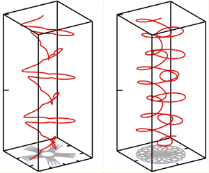
We illustrate the overall motion of the disk in the laboratory frame in figure 7 where we plot selected paths in the  $(\chi _{pitch},\chi _{roll})$-phase space (figure 7a–d), the corresponding trajectories of the disk's centre of mass,
 $\boldsymbol {r}_M(t)$, (figure 7e–h), and the time-traces of the disk's three Tait–Bryan angles (figure 7i–l). In each case, the disk is released at the origin,
 $\boldsymbol {r}_{M}^{[0]}=\boldsymbol {0}$, with zero yaw angle,
 $\chi _{yaw}^{[0]}=0$ (or, equivalently,
 $\chi _{yaw}^{[0]}=2{\rm \pi}$) and
 $\chi _{roll}^{[0]} = {\rm \pi}/2$. The plots show the trajectories resulting from four different initial values for the pitch angle. In figure 7(a) we start with a small value,
 $\chi _{pitch}^{[0]}=10^{-4}{\rm \pi}$, which results in a path close to the outermost boundary of the accessible phase plane, and a motion that alternates distinctly between pitching and rolling, with very little change to the yaw angle. (Note that
 ${\rm d}\chi _{yaw}/{\rm d}t|_{t=0} < 0$, therefore the yaw angle (which we normalised to be in the range
 $[0,2{\rm \pi} ]$) starts at
 $\chi _{yaw}^{[0]}=2{\rm \pi}$; similarly
 $\chi _{yaw}$ jumps by
 $2{\rm \pi}$ whenever
 $\chi _{yaw}$ is about to become negative.) Key points on the disk's trajectory are identified by the same labels as in figures 4 and 5: from A to B, the disk reorients predominantly by pitching; as discussed above, the rapid, approximately equal and opposite change to the roll and yaw angles when
 $\chi _{pitch}$ is close to
 ${\rm \pi} /2$ (from B to E) does not lead to a significant reorientation of the disk, and the pitching motion then continues from E to F. The disk then rights itself by rolling, via the path from F to
 ${\rm A}'$ in the phase plane. The disk now has retained its original inclination but is rotated by approximately 180
 $^\circ$ about the direction of gravity; a second loop around the phase plane, from
 ${\rm A}'$ to
 ${\rm A}''$, then returns the disk close to its original orientation.
The paths in the phase plane (a–d) for a disk released at the origin,  $\boldsymbol {r}_{M}^{[0]}=\boldsymbol {0}$, with
 $\chi _{yaw}^{[0]}=0$,
 $\chi _{roll}^{[0]} = {\rm \pi}/2$ and (a)
 $\chi _{pitch}^{[0]} = 10^{-4}{\rm \pi}$; (b)
 $\chi _{pitch}^{[0]} = \chi _{pitch}^{[centre]}-0.1{\rm \pi}$; (c)
 $\chi _{pitch}^{[0]} = \chi _{pitch}^{[centre]}-0.01{\rm \pi}$; (d)
 $\chi _{pitch}^{[0]} = \chi _{pitch}^{[centre]}$. The corresponding trajectories of the centre of mass in the laboratory frame of reference (e–h) and the time-evolution of the Tait–Bryan angles
 $\chi _{pitch}$ (black),
 $\chi _{roll}$ (blue) and
 $\chi _{yaw}$ (red) (i–l), respectively. See the supplementary material for animations of these figures available at https://doi.org/10.1017/jfm.2024.923.

During the pitching dominated phases, the horizontal drift of the disk's centre of mass is predominantly in the body-frame  $x_2$-direction, while it drifts predominantly in the
 $x_1$-direction when reorienting by rolling. Given that at the end of the first loop around the phase plane (from A to
 ${\rm A}'$), the disk has rotated by approximately 180
 $^\circ$ about the vertical axis, the direction of the horizontal drift during the second loop (from
 ${\rm A}'$ to
 ${\rm A}''$) occurs in the opposite direction. As a result, the projection of the trajectory onto the laboratory's
 $(x_1,x_2)$-plane (shown with grey lines in figure 7e–h) is approximately cross-shaped.
The reorientation by pitching can be seen to occur much more slowly than by rolling, consistent with the relative magnitudes of the rolling- and pitching-induced torques shown in figure 3, so the disk spends the majority of its time performing a slow pitching-dominated motion. During this phase, most paths in the phase plane (apart from those in the vicinity of the centre), converge towards a narrow region near  $\chi _{roll} \approx 0,{\rm \pi}$, see figure 5. This implies that during this phase, the disk is highly sensitive to perturbations in the roll angle. Small perturbations introduced by the numerical integration of the governing equations can therefore result in large deviations in the paths on later parts of the orbit. Such numerical perturbations were controlled by performing the time integration with sufficiently small time steps; the fact that the paths close confirms the accuracy of the computations. However, in laboratory experiments physical perturbations are unavoidable, and as a result it is unlikely that such exactly closed orbits will be observable experimentally. This is consistent with the experimental observations by Miara et al. (Reference Miara, Vaquero-Stainer, Pihler-Puzović, Heil and Juel2024).
In figure 7(b) we start with a larger initial pitching angle,  $\chi _{pitch}^{[0]}=\chi _{pitch}^{[centre]}-0.1{\rm \pi}$ for which the trajectory is closer to the interior of the phase plane. Pitching and rolling therefore occur continuously and the changes in
 $\chi _{pitch}$ and
 $\chi _{roll}$ induce a concomitant change in the yaw angle. Again
 $\chi _{roll}$ and
 $\chi _{yaw}$ undergo rapid opposing changes without any significant reorientation of the disk whenever
 $\chi _{pitch}$ approaches
 ${\rm \pi} /2$.
In figure 7(c) we start with a pitching angle close to the centre,  $\chi _{pitch}^{[0]}=\chi _{pitch}^{[centre]}-0.01{\rm \pi}$ where
 $\chi _{pitch}^{[centre]} = 0.44{\rm \pi}$. In the phase plane, the trajectory therefore remains close to the centre, with the reorientation dominated by small, periodic oscillations in roll angle, accompanied by a near constant rate of change in
 $\chi _{yaw}$; see the time-trace of the Tait–Bryan angles at the bottom of the figure. The changes in roll and pitch angles in figures 7(b) and 7(c) lead to a continual change in the direction of the horizontal drift, resulting in a spirograph-like patterns in the projection of the trajectories onto the laboratory
 $(x_1,x_2)$-plane.
Finally, in figure 7(d) the disk is released with  $( \chi _{pitch}^{[0]},\chi _{roll}^{[0]}) = (\chi _{pitch}^{[centre]},\chi _{roll}^{[centre]})$. Pitch and roll angles therefore remain constant while the yaw angle decreases at a constant rate, according to
 ${\rm d} \chi _{yaw}/{\rm d}t = f_{yaw}(\chi _{pitch}^{[centre]},\chi _{roll}^{[centre]})$. The ODE (3.7) for
 ${\rm d}\boldsymbol {r}_M/{\rm d}t$ then implies that the velocity of the disk's centre of mass varies periodically with the period of the yawing motion, resulting in a spiral trajectory in the laboratory frame and a circular projection onto the laboratory
 $(x_1,x_2)$-plane.
The supplementary material for this paper provides animations that illustrate the sedimentation of the disks along the trajectories shown in figure 7.
4.5. Dependence on the disk's radius of curvature
So far, we have focused on the motion of a U-shaped disk with a given radius of curvature. We found the behaviour of that disk to be fundamentally different from its flat equivalent: as mentioned in § 1, flat circular disks that sediment in an unbounded fluid at zero Reynolds number neither rotate nor change their inclination, and continue to drift in a fixed horizontal direction while sedimenting. The question therefore arises how these different behaviours can be reconciled in the limit as  $R_c \to \infty$, i.e. when the U-shaped disk turns into a flat one.
Figure 8(a) shows that, qualitatively, the phase plane describing the disk's inclination remains the same when we change the disk's radius of curvature: the inclination still undergoes periodic changes, with the paths in the  $(\chi _{pitch} ,\chi _{roll})$-phase plane following closed orbits around their respective centres. However, the rate at which the disk reorients decreases with an increase in
 $R_c$. This is illustrated in figure 8(b) where we plot
 \begin{equation} T_{period} = 2{\rm \pi} \left( \left. \frac{{\rm d}\chi_{yaw}}{{\rm d}t} \right|_{\left(\chi_{pitch}^{[centre]},\chi_{roll}^{[centre]}\right)} \right)^{{-}1}, \end{equation}
which is the time it takes for the disk to rotate by  $360^\circ$ about the direction of gravity when sedimenting along its spiral path at a fixed inclination. The solid line is a power-law curve fit to the computational data and suggests that
 $T_{period} \sim R_c^{1.63}$ as
 $R_c \to \infty$. Thus, nearly flat disks (with a very large radius of curvature) still move around their periodic orbits in the phase plane, but they do so increasingly slowly, so that their inclination remains approximately (and, in the actual limit
 $R_c \to \infty$, exactly) constant.
(a) Plot of the paths in the  $(\chi _{roll},\chi _{pitch})$-phase plane for disks of different radii of curvature (black,
 $R_c = 0.35$; red,
 $R_c = 0.5$; blue,
 $R_c = 2$). (b–d) Plots illustrating (b) the time
 $T_{period}$ for the periodic reorientation of the sedimenting disk, (c) the approach of
 $\chi _{pitch}^{{[centre]}}$ to
 ${\rm \pi} /2$, and (d) the Frobenius norm of the coupling tensor, all as a function of the disk's radius of curvature,
 $R_c$.

This behaviour is reflected in the fact that the entries in the off-diagonal coupling block,  $\boldsymbol {C}_M$, in the resistance matrix go to zero as the radius of curvature increases. This is illustrated in figure 8(d) by the plot of the Frobenius norm
 $||\boldsymbol {C}_M||_F = (\sum _i\sum _jC_{M,ij}^2)^{1/2}$ as a function of
 $R_c$ which can also be seen to follow an approximate power-law behaviour, with
 $||\boldsymbol {C}_M||_F \sim R_c^{-1}$, so that when
 $R_c \to \infty$ translational motions no longer induce rotations (and vice versa).
One possible interpretation of these results is that in the limit  $R_c \to \infty$, any initial inclination
 $(\chi _{pitch}^{[0]},\chi _{roll}^{[0]})$ becomes a fixed point in the sense that the motion along the paths in the
 $(\chi _{pitch},\chi _{roll})$-phase plane becomes infinitely slow. However, it is also of interest to see what happens to the centres (which are always fixed points) as the disk's radius of curvature is increased. Equation (4.2a,b) showed that
 $\chi _{roll}^{[centre]} = {\rm \pi}/2$, irrespective of the disk's radius of curvature, while
 $\chi _{pitch}^{{[centre]}}$ depends on the ratio of the coefficients
 $\mathbb {B}$ and
 $\mathbb {D}$, both of which are given in terms of the coefficients of the resistance matrix in Appendix B. As
 $R_c \to \infty$, the coefficients of the sub-blocks
 $\boldsymbol {K}$ and
 $\boldsymbol{\varOmega }_M$ approach the finite values for a flat disk (see figure 10 below) while the non-zero coefficients in the coupling matrix
 $\boldsymbol {C}_M$ go to zero, as shown in figure 8(d). However,
 $C_{12}$ goes to zero much more quickly than
 $C_{21}$ (the data suggests that
 $C_{12} \sim R_c^{-3}$ while
 $C_{21} \sim R_c^{-1}$ as
 $R_c \to \infty$ which implies that
 $\chi _{pitch}^{{[centre]}} \to {\rm \pi}/2$ as
 $R_c \to \infty$, consistent with the behaviour observed in figure 8(a), where the centres move towards the right as
 $R_c$ is increased (see also the plot of
 $\chi _{pitch}^{{[centre]}}$ as a function of
 $R_c$ in figure 8c).
To interpret this result we note that for  $\chi _{roll} = \chi _{roll}^{[centre]} = {\rm \pi}/2$ the body-fitted normal
 $\boldsymbol {n}^{{\mathcal {F}}_b}$ (pointing in the direction of
 $x_3^{{\mathcal {F}}_b}$) is oriented parallel to the laboratory frame
 $(x_1,x_2)$-plane, i.e.
 $\boldsymbol {n}^{{\mathcal {F}}_b} \boldsymbol {\cdot } \boldsymbol {e}_3 = 0$. When the disk is in this orientation, the continuous change to
 $\chi _{yaw}$ introduces a rigid body rotation about
 $x_3$, while a change to
 $\chi _{pitch}^{{[centre]}}$ rotates the disk about
 $\boldsymbol {n}^{{\mathcal {F}}_b}$ (recall again that the Tait–Bryan angles describe rotations that have to be applied consecutively, in the order
 ${\rm yaw}\rightarrow {\rm pitch}\rightarrow {\rm roll}$).
The effect of changes to the disk's radius of curvature on its orientation as it sediments along the spiral trajectory associated with  $(\chi _{pitch}^{{[centre]}}(R_c),\chi _{roll}^{{[centre]}} = {\rm \pi}/2 )$ is illustrated in figure 9: for a tightly curved disk, the body-fitted roll axis,
 $x_2^{{\mathcal {F}}_b}$, is strongly inclined away from the direction of gravity and the disk sediments along a wide spiral trajectory; see the black disk and the associated black dotted line which shows the trajectory of that disk's centre of mass in the laboratory frame. As the radius of curvature increases and
 $\chi _{pitch}^{{[centre]}} \to {\rm \pi}/2$, the disk rights itself and its roll axis approaches the
 $x_3$-axis in the laboratory frame (red and blue disks). As it approaches this configuration, the horizontal velocities go to zero while the vertical velocity approaches the finite sedimentation speed of a flat disk in its edge-on configuration. This leads to an increase in the pitch of the spiral trajectories whose radius (in the
 $(x_1,x_2)$-plane) shrinks to zero. Thus, in the limit as
 $R_c \to \infty$, a disk that sediments along the (nominally) spiral trajectory associated with the centre in the
 $(\chi _{pitch},\chi _{roll})$-phase plane sediments purely vertically, and in an edge-on orientation.
The helical trajectories of three disks with different curvatures, all released from  $\boldsymbol {r}_M^{[0]}= \boldsymbol {0}$ (green sphere), with an initial inclination
 $( \chi _{pitch}^{[0]},\chi _{roll}^{[0]}) = (\chi _{pitch}^{[centre]}(R_c),\chi _{roll}^{[centre]} = {\rm \pi}/2)$. The disk's inclination remains constant and it sediments along helical trajectories. The inset shows the inclination of the disks relative to the direction of gravity; (black,
 $R_c = 0.35$; red,
 $R_c = 0.5$; blue,
 $R_c = 2$.) As
 $R_c \to \infty$ the helical trajectories associated with this particular inclination degenerate to a straight vertical line and the disk sediments in an edge-on orientation.

5. Discussion and conclusions
We have studied the sedimentation of U-shaped rigid disks at zero Reynolds number and shown that, despite their non-chiral shape, they tend to sediment along complex spiral paths whose chirality depends on the disks’ initial orientation. We showed this to be due to the fact that the purely vertical sedimentation of such disks in their upright U orientation is stable (unstable) to perturbations about their roll (pitch) axes, with the reverse being true when they sediment in an upside-down U orientation. The instabilities cause the disks to continuously reorient by undergoing alternating rolling- and pitching-dominated rotations which are accompanied by a periodically varying horizontal drift. During each roll/pitch cycle, the disk performs a net rotation about the direction of gravity, which is generally an irrational multiple of  ${\rm \pi}$. The combination of these effects results in complex spiral trajectories, similar to those we observed in our experimental study (Miara et al. Reference Miara, Vaquero-Stainer, Pihler-Puzović, Heil and Juel2024).
The analysis was greatly facilitated by the fact that the numerical solution of the 3-D Stokes equations showed that wall effects (arising from a finite computational domain or, in an experiment, the finite size of the tank) only have a small effect on the pitching and rolling instabilities that are responsible for the disk's behaviour. This allowed us to analyse the disk's sedimentation in an unbounded fluid, using resistance matrices computed in finite domains. While this already led to a significant reduction in the computational effort (compared with time stepping the motion of the disk in the 3-D fluid domain), a further key simplification arose from the fact that for sedimentation in an unbounded fluid, only two of the disk's six rigid-body degrees of freedom (comprising the position of the disk's centre of mass and its orientation, the latter described in terms of three Euler angles) are genuine degrees of freedom. This allowed us to study the dynamics of the disk's sedimentation in a two-dimensional phase space comprising the Tait–Bryan pitch and roll angles. In this phase space, the periodic rolling–pitching reorientations appear as closed orbits. They enclose a centre which corresponds to the special case in which the disk sediments along a perfectly helical path while rotating at a fixed rate about the direction of gravity.
The behaviour of rigid U-shaped disks is therefore fundamentally different from that of their flat counterparts which maintain their inclination, and generally sediment with a constant horizontal drift. The latter effect causes dilute clouds of sedimenting flat disks to disperse horizontally; our findings imply that clouds of U-shaped disks will not spread horizontally.
The difference in the behaviour of the two types of disks must, of course, disappear when the curvature of the U-shaped disk is reduced to zero. We showed that the rate at which U-shaped disks reorient decreases with a reduction in their curvature, so that in the limit of zero curvature the disk's initial inclination changes infinitely slowly and thus remains constant.
We focused on the sedimentation of U-shaped disks because their shape resembles that observed for elastic disks in preliminary experiments by Miara (Reference Miara2024) and also in recent computations by Yu & Graham (Reference Yu and Graham2024) who found that, qualitatively, initially planar elastic sheets tended to deform into such shapes as they sediment.
The actual shape of a sedimenting elastic sheets is, of course, determined by the fluid traction acting on them, and therefore has to be obtained via the solution of a fully coupled, and in general time-dependent, fluid–structure interaction problem. However, thin elastic sheets have an extensional (membrane/in-plane) stiffness that is much larger than their bending stiffness. Therefore, they tend to deform approximately isometrically, with little in-plane stretching. This restricts the types of shapes that sedimenting elastic sheets can adopt. Our results suggest that once the sheet has deformed and reoriented itself into an upright U-shape, it will become subject to the (relatively slow) rotational instability about the pitching axis. This implies that, counter to the conjecture by Yu & Graham (Reference Yu and Graham2024), the upright U-shape is not actually a stable configuration for elastic sheets.
Supplementary movie
A supplementary movie is available at https://doi.org/10.1017/jfm.2024.923. This supplementary movie provides an animation of the static graphics shown in figure 7; it shows the trajectories of the disk's orientation through the pitch–roll phase-space, synchronised in time with the physical rigid-body dynamics in the lab frame. The initial conditions and therefore the subsequent trajectories correspond exactly to those shown in figure 7. In the lower animations, the disk's body-fitted axes are shown, centred on the centre of mass, with the dark blue arrows corresponding to the pitch axes,  $x_1^{{\mathcal {F}}_b}$, the cyan arrows corresponding to the roll axes,
 $x_2^{{\mathcal {F}}_b}$, and the magenta arrows corresponding to their cross product. The 3-D path of the centre of mass is shown by a yellow–red trace, coloured by vertical depth, and its projection onto the
 $x_1$–
 $x_2$ plane is shown by the red trace. With the exception of the left-most animation, the disks are unscaled in the
 $x_1$–
 $x_2$ directions, but are scaled appropriately in the
 $x_3$ direction so as to provide an orthographic projection of the disk on screen; the disks’ visible extent in the
 $x_3$ direction is therefore not representative and is merely for illustrative purposes. Owing to the correct
 $x_1$–
 $x_2$ scaling, the rightmost three disks appear different in size as a result of the different axis-limits chosen for the
 $x_1$–
 $x_2$ extent of the trajectories. The leftmost animation is, however, scaled by a factor of 10 for visual clarity, since the very large distances traversed in the
 $x_2$ direction would render the disk difficult to interpret if left unscaled. The effective frame-rate of this leftmost animation is also multiplied by a factor of three relative to the other animations, since there is a much greater orbital time period associated with trajectories very close to outermost limit, as evidenced in the animated phase-space traces above. It can be readily observed that the leftmost disk spends large periods of time translating near vertically in orientations which correspond to regions of the phase-space close to the saddle points (labelled as A and F in figure 7) as a result of the very small initial perturbation from the upright U orientation.
Funding
C.V.-S. and T.M. were funded by EPSRC DTP studentships. A.J. acknowledges funding by EPSRC (grant EP/T008725/1).
Declaration of interests
The authors report no conflict of interest.
Appendix A. Derivation of the evolution equations in an unbounded fluid
Figure 1 shows how the disk's orientation is described in terms of an intrinsic sequence of rotations by the Tait–Bryan angles  $\chi _{yaw}$,
 $\chi _{pitch}$ and
 $\chi _{roll}$. Starting from a reference orientation in which the disk's principal axes are aligned with the Cartesian coordinates
 $(x_1^{{\mathcal {F}}_{lab}}, x_2^{{\mathcal {F}}_{lab}},x_3^{{\mathcal {F}}_{lab}})$ in the laboratory frame,
 ${\mathcal {F}}_{lab}$, we apply rotations about the three coordinate axes, but in subsequent frames, so that
 \begin{equation} {{\mathcal{F}}_{lab}} = {{\mathcal{F}}_0} \stackrel{ {\chi_{yaw}\ \text{about}\ x_3^{{\mathcal{F}}_{lab}}}}{ \xrightarrow{} } {{\mathcal{F}}_{1}} \stackrel{{\chi_{pitch}\ \text{about}\ x_2^{{\mathcal{F}}_{1}}}}{ \xrightarrow{} } {{\mathcal{F}}_{2}} \stackrel{ {\chi_{roll}\ \text{about}\ x_1^{{\mathcal{F}}_{2}}}}{ \xrightarrow{} } {{\mathcal{F}}_{3}}= {{\mathcal{F}}_{b}} . \end{equation}
Given a vector  $\boldsymbol {a}$ with components
 $a_i^{{\mathcal {F}}_{j}}$ in frame
 ${\mathcal {F}}_{j}$, its components in the subsequent frame are given by
 \begin{equation} \left[ a_{1}^{{\mathcal{F}}_{j+1}}, a_{2}^{{\mathcal{F}}_{j+1}}, a_{3}^{{\mathcal{F}}_{j+1}} \right]^{\rm T} = {\mathcal{R}}_{{\mathcal{F}}_{j}}^{{\mathcal{F}}_{j+1}} \left[ a_{1}^{{\mathcal{F}}_{j}}, a_{2}^{{\mathcal{F}}_{j}}, a_{3}^{{\mathcal{F}}_{j}} \right]^{\rm T}, \end{equation}
where the matrices  ${\mathcal {R}}_{{\mathcal {F}}_{j}}^{{\mathcal {F}}_{j+1}}$ are standard orthogonal rotation matrices, e.g.
 \begin{equation}
{\mathcal{R}}_{{\mathcal{F}}_{0}}^{{\mathcal{F}}_{1}}
=\left( \begin{array}{@{}c@{\quad}c@{\quad}c@{}} \cos(\chi_{yaw}) &
\sin(\chi_{yaw}) & 0 \\ -\sin(\chi_{yaw}) &
\cos(\chi_{yaw}) & 0 \\ 0 & 0 & 1 \end{array}
\right)\quad\mbox{with}\
{\mathcal{R}}_{{\mathcal{F}}_{1}}^{{\mathcal{F}}_{0}} =
\left({\mathcal{R}}_{{\mathcal{F}}_{0}}^{{\mathcal{F}}_{1}}\right)^{{-}1}
=
\left({\mathcal{R}}_{{\mathcal{F}}_{0}}^{{\mathcal{F}}_{1}}\right)^{{\rm
T}}, \end{equation}
and each of these matrices depend only on the single angle describing the associated rotation. Thus, translating the velocity of the disk's centre of mass from  ${\mathcal {F}}_{lab}$ to
 ${\mathcal {F}}_{b}$ is achieved by
 \begin{equation} \left[ U_{1}^{{\mathcal{F}}_{b}}, U_{2}^{{\mathcal{F}}_{b}}, U_{3}^{{\mathcal{F}}_{b}} \right]^{\rm T} = {\mathcal{R}}_{{\mathcal{F}}_{lab}}^{{\mathcal{F}}_{b}} \left[ U_{1}^{{\mathcal{F}}_{lab}}, U_{2}^{{\mathcal{F}}_{lab}}, U_{3}^{{\mathcal{F}}_{lab}} \right]^{\rm T}, \end{equation}
where
 \begin{equation} {\mathcal{R}}_{{\mathcal{F}}_{lab}}^{{\mathcal{F}}_{b}} = {\mathcal{R}}_{{\mathcal{F}}_{2}}^{{\mathcal{F}}_{b}} {\mathcal{R}}_{{\mathcal{F}}_{1}}^{{\mathcal{F}}_{2}} {\mathcal{R}}_{{\mathcal{F}}_{lab}}^{{\mathcal{F}}_{1}}. \end{equation}
Furthermore, the rate of change in the Tait–Bryan angles (which perform rigid body rotations about coordinate axes aligned with subsequent frames, see (A1)) results in an overall rate of rotation  $\boldsymbol{\omega }$ whose components in the body frame are
 \begin{align} \left[\omega_{1}^{{\mathcal{F}}_{b}}, \omega_{2}^{{\mathcal{F}}_{b}}, \omega_{3}^{{\mathcal{F}}_{b}} \right]^{\rm T} & = {\mathcal{R}}_{{\mathcal{F}}_{2}}^{{\mathcal{F}}_{b}} {\mathcal{R}}_{{\mathcal{F}}_{1}}^{{\mathcal{F}}_{2}} \ \left[ 0,0,\frac{{\rm d}\chi_{yaw}}{{\rm d}t} \right]^{\rm T} +{\mathcal{R}}_{{\mathcal{F}}_{2}}^{{\mathcal{F}}_{b}} \left[ \frac{{\rm d}\chi_{pitch}}{{\rm d}t}, 0, 0 \right]^{\rm T} +\left[ 0,\frac{{\rm d}\chi_{roll}}{{\rm d}t}, 0 \right]^{\rm T}\nonumber\\ & = {\mathcal{S}} \left[\frac{{\rm d}\chi_{pitch}}{{\rm d}t}, \frac{{\rm d}\chi_{roll}}{{\rm d}t}, \frac{{\rm d}\chi_{yaw}}{{\rm d}t} \right]^{\rm T}, \end{align}
where
 \begin{equation} {\mathcal{S}} = \left(
\begin{array}{@{}c@{\quad}c@{\quad}c@{}} \cos(\chi_{roll}) & 0 &
-\cos(\chi_{pitch})\sin(\chi_{roll}) \\ 0 & 1 &
\sin(\chi_{pitch}) \\ \sin(\chi_{roll}) & 0 &
\cos(\chi_{pitch})\cos(\chi_{roll}) \end{array} \right)
\end{equation}
which is independent of  $\chi _{yaw}$.
This allows us to transform (2.6) into quantities in the laboratory frame of reference,
 \begin{align} &\left(\begin{array}{@{}c@{}}
{\mathcal{R}}_{{\mathcal{F}}_{2}}^{{\mathcal{F}}_{b}}(\chi_{roll})
{\mathcal{R}}_{{\mathcal{F}}_{1}}^{{\mathcal{F}}_{2}}(\chi_{pitch})
{\mathcal{R}}_{{\mathcal{F}}_{lab}}^{{\mathcal{F}}_{1}}(\chi_{yaw})\left[
\dfrac{{\rm d}r_{M,1}^{{\mathcal{F}}_{lab}}}{{\rm d}t},
\dfrac{{\rm d}r_{M,2}^{{\mathcal{F}}_{lab}}}{{\rm d}t},
\dfrac{{\rm d}r_{M,3}^{{\mathcal{F}}_{lab}}}{{\rm d}t}
\right]^{\rm T} \\ {\mathcal{S}}(\chi_{pitch},
\chi_{roll}) \left[ \dfrac{{\rm d}\chi_{pitch}}{{\rm d}t},
\dfrac{{\rm d}\chi_{roll}}{{\rm d}t}, \dfrac{{\rm
d}\chi_{yaw}}{{\rm d}t} \right]^{\rm T} \end{array} \right)
\nonumber\\ &\quad = \begin{pmatrix} \boldsymbol{K} &
\boldsymbol{C}_M^T \\ \boldsymbol{C}_M &
\boldsymbol{\varOmega}_M \end{pmatrix}^{{-}1}\left(
\begin{array}{c}
{\mathcal{R}}_{{\mathcal{F}}_{2}}^{{\mathcal{F}}_{b}}(\chi_{roll})
{\mathcal{R}}_{{\mathcal{F}}_{1}}^{{\mathcal{F}}_{2}}(\chi_{pitch})
{\mathcal{R}}_{{\mathcal{F}}_{\rm
lab}}^{{\mathcal{F}}_{1}}(\chi_{yaw})
\left[F_1^{{\mathcal{F}}_{lab}}, F_2^{{\mathcal{F}}_{lab}},
F_3^{{\mathcal{F}}_{lab}} \right]^{\rm T} \\[9pt]
{}{\mathcal{R}}_{{\mathcal{F}}_{2}}^{{\mathcal{F}}_{b}}(\chi_{roll})
{\mathcal{R}}_{{\mathcal{F}}_{1}}^{{\mathcal{F}}_{2}}(\chi_{pitch})
{\mathcal{R}}_{{\mathcal{F}}_{lab}}^{{\mathcal{F}}_{1}}(\chi_{yaw})
\left[ T_{pitch}^{{\mathcal{F}}_{lab}},
T_{roll}^{{\mathcal{F}}_{lab}},
T_{yaw}^{{\mathcal{F}}_{lab}} \right]^{\rm T} \end{array}
\right), \end{align}
which is easily rewritten in the form (3.2). The reason for keeping the equations in this form, and for spelling out explicitly the dependence of the rotation matrices on the various Tait–Bryan angles is that it shows that the equations are not affected by rigid body translations,  $r_{M,i}^{{\mathcal {F}}_{lab}}(t) \to r_{M,i}^{{\mathcal {F}}_{lab}}(t) + \delta r_{M,i}^{{\mathcal {F}}_{lab}}$ for arbitrary constants
 $\delta r_{M,i}^{{\mathcal {F}}_{lab}}$, because none of the coefficients depend on the position of the disk. Furthermore, since for free sedimentation we have
 $[F_1^{{\mathcal {F}}_{lab}}, F_2^{{\mathcal {F}}_{lab}}, F_3^{{\mathcal {F}}_{lab}}] = [0,0,-{\rm \pi} h/{{\mathcal {L}}}]$ and
 $T_{\{{roll,pitch,yaw}\}}^{{\mathcal {F}}_{lab}}=0$, a change in the yaw angle by an arbitrary constant
 $\delta \chi _{yaw}$ so that
 $\chi _{yaw}(t) \to \chi _{yaw}(t) + \delta \chi _{yaw}$, corresponding to a rigid body rotation about the vertical axis, does not affect the right-hand side, while on the left-hand side it simply subjects the trajectory to a rigid body rotation by that same angle, i.e.
 $[ r_{M,1}^{{\mathcal {F}}_{b}}(t), r_{M,2}^{{\mathcal {F}}_{b}}(t), r_{M,3}^{{\mathcal {F}}_{b}}(t) ]^{\rm T} \to {\mathcal {R}}_{lab}^{1}(\delta \chi _{yaw}) \ [ r_{M,1}^{{\mathcal {F}}_{b}}(t), r_{M,2}^{{\mathcal {F}}_{b}}(t), r_{M,3}^{{\mathcal {F}}_{b}}(t) ]^{\rm T}$. Thus, of the six initial conditions required for the solution of the governing equations, four translate into trivial rigid body modes. The shape of the trajectory and the rate at which the disk reorients relative to the direction of gravity while its centre of mass sediments along that path depend only on the initial values for the pitch and roll angles.
In fact, these two angles are the system's only genuine degrees of freedom: given the structure of  ${\mathcal {R}}_{{\mathcal {F}}_{lab}}^{{\mathcal {F}}_{1}}(\chi _{yaw})$, the right-hand side of (A8) depends only on
 $\chi _{pitch}$ and
 $\chi _{roll}$, and it has non-zero entries only in the first three rows. This implies that
 $\chi _{pitch}$ and
 $\chi _{roll}$ can be determined independently from the fourth and fifth row of the ODE system (A8) since these ODEs do not involve
 $r_{M,i}^{{\mathcal {F}}_{lab}}(t)$ and
 $\chi _{yaw}$. This leads to (3.3a,b). The evolution of the yaw angle
 $\chi _{yaw}(t)$ and the position of the centre of mass,
 $r_{M,i}^{{\mathcal {F}}_{lab}}(t)$, can then be determined a posteriori from the remaining four ODEs ((3.6) and (3.7) in § 3.2).
Appendix B. The structure of the resistance matrix and the derived quantities
The U-shaped disks considered in this study have two mutually orthogonal planes of symmetry. Happel & Brenner (Reference Happel and Brenner1983) show that for objects of this type the translation, rotation and coupling tensors have the form
 \begin{equation} \left.\begin{gathered} \boldsymbol{K} = \begin{pmatrix} K_{11} & 0 & 0 \\ 0 & K_{22} & 0 \\ 0 & 0 & K_{33} \end{pmatrix},\quad (\boldsymbol{\varOmega}_M) = \begin{pmatrix} \varOmega^{(M)}_{11} & 0 & 0 \\ 0 & \varOmega^{(M)}_{22} & 0 \\ 0 & 0 & \varOmega^{(M)}_{33} \end{pmatrix}, \\ \boldsymbol{C}_M = \begin{pmatrix} 0 & C^{(M)}_{12} & 0 \\ C^{(M)}_{21} & 0 & 0 \\ 0 & 0 & 0 \end{pmatrix}. \end{gathered}\right\} \end{equation}
The two diagonal blocks  $\boldsymbol {K}$ and
 $\boldsymbol {\varOmega }_M$ of the resistance matrix are diagonal, just as in the case of a flat disk. The key difference, which gives rise to non-trivial dynamics, arises from the translation–rotation coupling described by
 $\boldsymbol {C}_M$. For flat disks we have
 $\boldsymbol {C}_M = \boldsymbol {0}$, allowing them to sediment along simple, rotation-free trajectories. The fact that
 $C^{(M)}_{33}=0$ implies that our U-shaped disks can sediment along the body fitted
 $x_3^{\mathcal {F}_b}$ directions without reorienting or drifting sideways. This corresponds to the vertical sedimentation of the disk in its upright and upside-down U orientations. For all other orientations the non-zero entries in
 $\boldsymbol {C}_M$ imply that a translation in the
 $x_1^{\mathcal {F}_b}$ and
 $x_2^{\mathcal {F}_b}$ direction induce rotations about the
 $x_2^{\mathcal {F}_b}$ and
 $x_1^{\mathcal {F}_b}$ axes, respectively.
In terms of the non-zero entries in these three tensors, the coefficients featuring in the ODEs (3.3a,b), (3.6) and (3.7) in § 3.2 are then given by
 $$\begin{gather} \mathbb{B} = {K_{33}} \varOmega_{33} \left( {C_{12}}^{2} {C_{21}} + {C_{12}} \,{C_{21}}^{2} -{C_{12}} {K_{22}} \varOmega_{11} -{C_{21}} {K_{11}} \varOmega_{22} \right), \end{gather}$$
 $$\begin{gather}\mathbb{D} = {C_{21}} {K_{33}} \varOmega_{33} \left({C_{12}}^{2}-{K_{11}} \varOmega_{22}\right), \end{gather}$$
 $$\begin{gather}\mathbb{E} = \left({C_{21}}^{2} {K_{33}} -{K_{22}} {K_{33}} \varOmega_{11} \right) \left({C_{12}}^{2} \varOmega_{33} -{K_{11}} \varOmega_{22} \varOmega_{33} \right), \end{gather}$$
 $$\begin{gather}\mathbb{F} = \left({C_{21}}^{2}-{K_{22}} \varOmega_{11} \right) \left(\left({K_{33}} -{K_{11}} \right) \varOmega_{22} +{C_{12}}^{2}\right), \end{gather}$$
 $$\begin{gather}\mathbb{G} = \left({C_{21}}^{2}-{K_{22}} \varOmega_{11} \right) \left(\left({K_{33}} -{K_{11}} \right) \varOmega_{22} +{C_{12}}^{2}\right), \end{gather}$$
 $$\begin{gather}\mathbb{H} = {K_{33}} \left(\left(\left(-{K_{11}} +{K_{22}} \right) \varOmega_{11} -{C_{21}}^{2}\right) \varOmega_{22} +{C_{12}}^{2} \varOmega_{11} \right), \end{gather}$$
 $$\begin{gather}\mathbb{I} = {K_{33}} \left(\left(\left(-{K_{11}} +{K_{22}} \right) \varOmega_{22} +{C_{12}}^{2}\right) \varOmega_{11} -{C_{21}}^{2} \varOmega_{22} \right), \end{gather}$$
 $$\begin{gather}\mathbb{J} = {K_{33}} \varOmega_{11} \left({C_{12}}^{2}-{K_{11}} \varOmega_{22} \right), \end{gather}$$
 $$\begin{gather}\mathbb{K} = {K_{33}} \left({C_{21}}^{2}-{K_{22}} \varOmega_{11} \right) \left({C_{12}}^{2}-{K_{11}} \varOmega_{22} \right). \end{gather}$$
Appendix C. The importance of wall effects
The analysis presented in this paper relies heavily on the observation that wall effects only have a modest effect on the rolling and pitching behaviour of the disk. This allowed us to compute the resistance matrix for a disk sedimenting in an unbounded fluid by performing computations in a large but finite computational domain. The subsequent analysis was then performed by analysing the solutions of a small system of ODEs.
Given that in Stokes flow boundary effects are known to act over large distances, we briefly revisit the importance of the domain size (which features both in computations and in experiments) on our results. We showed in § 4.5 that the (in general) chiral sedimentation of U-shaped disks is due the non-zero off-diagonal blocks  $\boldsymbol {C}_M$ in the resistance matrix. We reconciled the behaviour of U-shaped disks with the flat counterpart by showing that these blocks to go zero as the disk's radius of curvature,
 $R_c$, increases. Figure 10(a) shows that the dependence of the off diagonal block
 $\boldsymbol {C}_M$ on the disk's radius of curvature is not visibly affected by an increase in the size of the computational domain. Conversely, the corresponding plots for the Frobenius norms of the two diagonal blocks
 $\boldsymbol {K}_M$ and
 $\boldsymbol{\varOmega }_M$ in figure 10(b) show that, as the disk's radius of curvature is increased, both norms approach constant values which are slightly above the theoretical values of
 $16 \sqrt {17}/3$ and
 $32 \sqrt {3}/3$ for a flat disk sedimenting in an unbounded fluid. The data computed in a domain of twice the (linear) size can be seen to be closer to the theoretical value for an unbounded fluid which is approached from above, indicating that the finite-size effects increase the translational and rotational drag (Brenner Reference Brenner1962; Caswell Reference Caswell1972).
The Frobenius norms of the submatrices  $\boldsymbol {K}, \boldsymbol {\varOmega }_M$ and
 $\boldsymbol {C}_M$, which comprise the resistance matrix, shown as a function of the radius of curvature of the disk and for box sizes
 $L=160$ (black ‘
 $+$’) and
 $L=320$ (red ‘
 $\times$’). (a) Log–log plot of the norm of the coupling tensor
 $\boldsymbol {C}_M$; the solid line shows a power-law fit to the final five data points, with the fitted exponent shown via the slope-triangle; (b) Semilogarithmic plot of the linear and rotational drag tensors
 $\boldsymbol {K}$ and
 $\boldsymbol {\varOmega }_M$; the dotted lines indicate the analytic values for a flat circular disk in an unbounded fluid.

To assess how this affects the disks’ behaviour figure 11 shows representative plots of (figure 11a) the trajectory of the disk's centre of mass, (figure 11b) the disk's closed orbits in the  $(\chi _{pitch},\chi _{roll})$-phase plane, and (figure 11c,d) the time evolution of the three Tait–Bryan angles. Solid and dashed lines represent the predictions obtained using the resistance matrix computed in domains of size
 ${\textit L} = 160$ and
 ${\textit L} = 320$, respectively. As anticipated from all the results presented so far, the
 $(\chi _{pitch},\chi _{roll})$-phase planes obtained from the two matrices are virtually identical. The slightly increased drag in the smaller domain results in small changes to the disk's predicted velocity, causing the two centre-of-mass trajectories shown in figure 11(a) to drift apart while the disk undergoes its periodic pitch–roll cycle. The time trace of the Tait–Bryan angles shows that the resistance matrix computed in the larger domain leads to a slight decrease in the period of the pitch–roll cycle which again causes the time-traces to drift apart. However, this has no effect on the qualitative behaviour within each roll-pitch cycle. This is illustrated by the close-up plot shown in figure 11(d), where the dash–dotted line was obtained by adding a suitable time offset to the dashed line in figure 11(c), so that the two time-traces are (re-)aligned at the beginning of that period. Following this realignment of the curves, the two time-traces are nearly indistinguishable again.
Trajectories for a disk with  $R_c=0.5$, released with initial conditions
 $\chi _{pitch}^{[0]} = 0.4{\rm \pi}, \chi _{roll}^{[0]} = 0.4{\rm \pi}$. Data was obtained with resistance matrices computed in domains of different sizes:
 $L = 160$ (solid) and
 $L = 320$ (dashed). (a) Trajectories of the centres of mass; (b) phase-space trajectory of the disk orientation; (c) time trace of the Tait–Bryan angles; (d) close-up time trace of the Tait–Bryan angles, with a time offset applied to the
 $L=320$ (dashed) trace to align the two trajectories at
 $\tilde {t} = 6.65$.

Appendix D. Validation
In order to construct a suitable validation case for our numerical scheme, we considered the special case of a flat, circular disk moving in an unbounded and otherwise quiescent fluid; for this case we have a closed-form exact solution  $(\boldsymbol {u}_{exact},p_{exact})$ (Happel & Brenner Reference Happel and Brenner1983), for which the force and torque on the disk are given by
 \begin{equation} \boldsymbol{F}_{exact} = \frac{16}{3} \begin{pmatrix} 2 & 0 & 0\\ 0 & 2 & 0 \\ 0 & 0 & 3 \end{pmatrix} \boldsymbol{\cdot}\boldsymbol{U}_M, \quad \boldsymbol{T}_{exact} = \frac{32}{3} \begin{pmatrix} 1 & 0 & 0\\ 0 & 1 & 0 \\ 0 & 0 & 1 \end{pmatrix} \boldsymbol{\cdot}\boldsymbol{\omega}. \end{equation}
We chose an arbitrary rigid body motion of the disk,  $\boldsymbol {U}_M = \{-0.7, -0.3, 0.6\}, \boldsymbol {\omega } =\{-3.1, 0.1, 0.9\}$, which we imposed via the boundary conditions (2.2) on the disk surface. On the outer boundaries of the computational domain (a cuboid of size
 $1.55\times 1.55 \times 0.55$) we applied the analytical velocity field as a Dirichlet conditions, except for the top surface where we imposed the analytical traction
 $\boldsymbol {\tau }_{exact} \boldsymbol {\cdot }\boldsymbol {n}$ as a Neumann condition. We then uniformly refined the mesh several times, and for each mesh computed the numerical solution using both classical Taylor–Hood elements and our augmented finite elements. The results of this convergence study are shown in figure 12, where we show the relative error between the analytical and computed values for drag and torque, obtained with both methods, as a function of the number of elements in the mesh. The figure demonstrates that the augmentation by singular functions described in § 3.1 not only outperforms the non-augmented elements by two orders of magnitude, but converges at a rate of more than twice the asymptotic order under mesh refinement.
Relative error (in per cent) of the computed drag (circles) and torque (squares) as a function of the mesh refinement, for a validation case in which a flat circular disk moves with  $\boldsymbol {U}_M = \{-0.7, -0.3, 0.6\}, \boldsymbol {\omega }=\{-3.1, 0.1, 0.9\}$. Filled symbols are for classical Taylor–Hood elements; hollow symbols are for the PDE-constrained solution where the velocity and pressure fields are augmented with appropriate singular functions, as described in § 3.1.


 Open access

