STANDARD MEASURES of POVERTY RELIEF

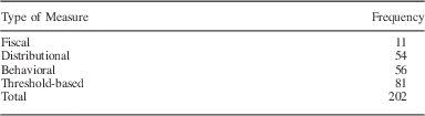
Social science traditionally relies on four broad strategies for characterizing social policy: fiscal, behavioral, distributional, and threshold-based measures (Table 1). Each measurement strategy offers analytic advantages, but also makes assumptions or obscures the effects of anti-poverty policy in ways that complicate substantive interpretations and comparative analysis. This paper begins by briefly describing each type of conventional measure. We focus more intently on the poverty reductions measures most closely related to our own poverty relief ratio and then use this discussion to motivate our measure of anti-poverty relief.

Table 1

Standard Measures of Poverty Relief in the Social Science Literature (2000–2012)

Note: This Table reports the type of measure used in the 68 articles analyzing social policy published in the social sciences between 2000 and 2012 and on JSTOR.

Fiscal measures report levels of government spending in social policy domains. Social expenditures, usually expressed as a percent of gross domestic product, are the most prominent of these fiscal measures, and scholars that use fiscal measures often implicitly assume that government spending directly, or at least disproportionately, benefits low-income households. However, there is evidence that fiscal measures do not straightforwardly measure redistribution or safety net program effectiveness (see Milanovic Reference Milanovic2000). For example, Moffitt and Sholz (Reference Moffitt and Scholz2009) find that in spite of increased social spending between 1984 and 2004, support for very poor families declined during this period. This likely reflects what Okun (Reference Okun1975) referred to as a “leaky bucket:” some of the money transferred from rich to poor “will simply disappear in transit” (quoted in Boadway and Keen Reference Boadway and Keen2000). Generally, fiscal measures are “input-oriented” and may insufficiently addressing the effects of social policy: who benefits and how much.

Distributional measures offer an alternative to fiscal measures and examine differences between labor market income and post-tax-and-transfer income distributions. Most often, Gini coefficients report the relationship between the cumulative income and the cumulative population rank distributions; the effects of redistribution are then measured as a proportion of market income inequality. Similar analyses use differences in the ratios of, for example, income at different percentiles of the distribution, or compare total income shares for high- and low-income earners. Notice, however, that distributional measures provide only limited information about the well-being of low-income households. Thompson and Smeeding (Reference Thompson and Smeeding2013), for example, combine their analysis of income inequality following the Great Recession with a separate analysis of poverty rates—both parts were necessary to show comprehensively the implications of the financial crisis. By focusing in the whole income distribution, distributional measures may therefore provide only limited information about the effects of policies for those at any specific place in the national income distributions.

Behavioral measures tie safety net program effectiveness to changes in, for example, program caseloads or the labor force participation rates of (former) safety net program participants (see e.g., Blank Reference Blank2002). Particularly following the Personal Responsibility and Work Opportunity Act (PRWOA) of 1996, which explicitly focused attention on behavioral outcomes like employment, recent analyses often use this measurement strategy to evaluate the effectiveness of current social policy. While behavioral measures have the advantage of tying program outcomes to specific program goals, there are at least two significant limitations: first, the relationship between behavioral outcomes and policy measures may be complicated by general economic conditions. Of the dramatic reduction in caseloads following welfare reform, for example, Lichter and Jayakody ask, “Is the decline in caseloads mostly due to the new welfare reform legislation or to a robust economy?” (Reference Lichter and Jayakody2002, 119). Second, the relationship between specific behaviors and economic well-being may be ambiguous. Some evidence suggests that while Temporary Assistance to Needy Families (TANF) programs (those implimented by the mid-1990s welfare reform) increase employment among low-income women, for example, significant proportions of welfare-to-work program participants have maintained incomes below the official poverty line (see e.g., Schoeni and Blank Reference Schoeni and Blank2000; Bavier Reference Bavier2001; Danziger et al. Reference Danziger, Heflin, Corcoran, Oltmans and Wang2002). Further, as Shaefer and Edin (Reference Shaefer and Edin2015) report, a focus on declining caseloads may obscure how TANF restrictions have forced increasing numbers of low-income households, particularly those with only tenuous connections to the labor market, into extreme poverty (see also Tach and Edin Reference Tach and Edin2017). For these reasons—complex relationships between policy and behavior, and ambiguous relationships between behavior and economic well-being—behavioral measures may provide limited or misleading information about the effectiveness of social policy.

Finally, the most commonly used measures for the analysis of social policy are threshold-based measures. As suggested above, threshold-based measures examine the frequency with which households earn less than some amount of income, believed necessary to meet basic needs, and characterize the difference between earnings and this specified amount (Ray Reference Ray2006). Of course, there is a large literature devoted to determining how this income amount—or threshold—ought to be calculated (for a recent summary, see Meyer and Sullivan Reference Meyer and Sullivan2012).Footnote ⁴ Nevertheless, empirical research on the United States typically uses (sometimes, percentages of) the official poverty line. Then, this class of measures reports estimates of the frequency of or weighted-average deviations from the poverty threshold. In their original formulation Foster, Greer and Thorbecke (Reference Foster, Greer and Thorbecke1984), for example, present the measure,

(1) $$P_{\gamma } \,{\equals}\,{1 \over n}\mathop{\sum}\limits_{i{\equals}1}^q \left( {{{\psi \,{\minus}\,y_{i} } \over \psi }} \right)^{\gamma } .$$

Here, ψ is the poverty threshold, y _i an individual’s income (ranked in increasing order of i), n the total population, and q the number of individuals with incomes less than ψ. Within this “Foster–Greer–Thorbecke (FGT)” framework, the impact of policy interventions is evaluated through the calculation of differences in P _γ , usually with parameter γ taking values <2. Notice that P ₀ gives the poverty rate, or the frequency with which individuals or households have incomes less than the poverty threshold. Further, P ₁ provides what is referred to as the poverty “gap,” or the average deviation of incomes from the poverty threshold (expressed as percentage of the poverty line) among low-income individuals or households. As γ increases, the earnings gap for the poorest household is weighted more heavily, and for this reason, within this literature, γ is referred to as the poverty aversion parameter.

Like the other measurement strategies considered here, the threshold-based measures offers important analytic advantages, as reflected by substantial, cumulative research building from Foster, Greer and Thorbecke’s (Reference Foster, Greer and Thorbecke1984) initial analysis. (For a discussion of this literature, see Foster, Greer and Thorbecke Reference Foster, Greer and Thorbecke2010.) However, as suggested above, and as should be obvious from Equation 1, comparisons across units or policies will be complicated by the relationship between q and ψ. That is, because the number of low-income households (q) will vary with poverty threshold (ψ), in ways that likely vary across observations, rankings of observations over P _γ will also vary with the poverty threshold, especially when γ=0 (i.e., poverty rates).Footnote ⁵ More extensive comparisons between the poverty relief ratio, $\scr R$ , and the FGT poverty gap measure will be made below; this brief discussion serves as an introduction to one of the key challenges associated with more standard threshold-based measures and an important justification for a new approach measuring the effectiveness of social policy.

MEASURING POVERTY RELIEF

In the United States, low-income households benefit from a portfolio of safety net programs, often administered at several different levels of government (for a discussion of the policy “patchwork,” see Moffitt and Scholz Reference Moffitt and Sholz2010). Program eligibility and benefit levels vary with earnings, even among low-income households. Further, because participation for some programs limits eligibility for others, the anti-poverty effectiveness of specific programs may be difficult to assess. Therefore, to understand American safety net effectiveness, we examine the total amount of transfers to low-income households.Footnote ⁶ Specifically, we use the relationship between total social transfers and total market income to derive summary statistics that characterize dimensions of safety net support in the United States. This section provides an overview of how these data are measured and some basic descriptive analysis; Appendix A (included in our on-line supplementary materials) reports more technical details.

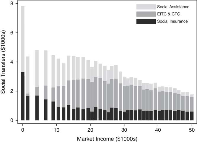
Figure 1 uses the CPS Annual Social and Economic (March) Supplement—our primary data source, and the best resource for cross-state analysis of household income dynamics—to estimate levels of social transfers by program type and market earnings. Here, we group social transfers into three program categories: social insurance, social assistance benefits, and refundable tax credits. Social insurance benefits include unemployment insurance and workers’ compensation. Social assistance amounts report traditional welfare benefits (e.g., TANF), as well as near-cash food and energy supplements. Finally, refundable tax credits include the earned income tax credit (EITC) and children’s tax credits (CTC), which are calculated by the US Census Bureau on the basis of information provided by respondents. The total working-aged household amounts of these social transfers—social insurance, social assistance, EITC, and CTC—are reported on the vertical axis of Figure 1. The horizontal axis reports working-aged household levels of market income, which include wages and salaries, income from self employment, farming, interest and dividends, rent, child support, alimony, veteran’s benefits, pension and retirement benefits (excluding social security), and assistance from friends and family members.Footnote ⁷

Fig. 1

Social transfers, by type and level of market earnings (2010–2014) Note: Figure 1 reports the relationship between social transfers by type and market income for the United States (2010–2014). Each bar represents the mean amount of social transfers for 1 percent of the pooled 2010–2014 sample. The main text provides details of program categories. All currency amounts are reported in thousands of 2014 US dollars. EITC=earned income tax credit; CTC=children’s tax credits.

Notice, in Figure 1, three dimensions of variation across market income levels: first, income groups vary in the total amount of support that they receive; those without market earnings received the largest amounts. Second, income groups vary in the programs they participate in: by design, households without market earnings do not receive EITC+CTC support. Third, low-income households vary in the composition of support they receive from each program type: compare, for example, income groups at the very low end of the income distribution. Those with no market earnings receive substantially more support from social assistance programs than households with slightly higher—but still very low—levels of market earnings. Here, we refer to the extent to which income support levels drop off with small differences in earnings as “relief falloff.”Footnote ⁸ When estimates of relief falloff are very high, this indicates that safety net support drops dramatically with small increases in earnings. Finally, Figure 1 demonstrates most clearly that attention to any one program, or even one type of program, provides an incomplete and potentially misleading impression of poverty relief in the United States. A focus on the effects of EITC, for example, ignores those households with no earnings. Similarly, an exclusive focus on TANF misses the anti-poverty relief the EITC provides to those who earn very little. Instead, comparative analysis of poverty relief ought to take a total income approach, that recognizes the varying structure of low-income households’ portfolios of support.

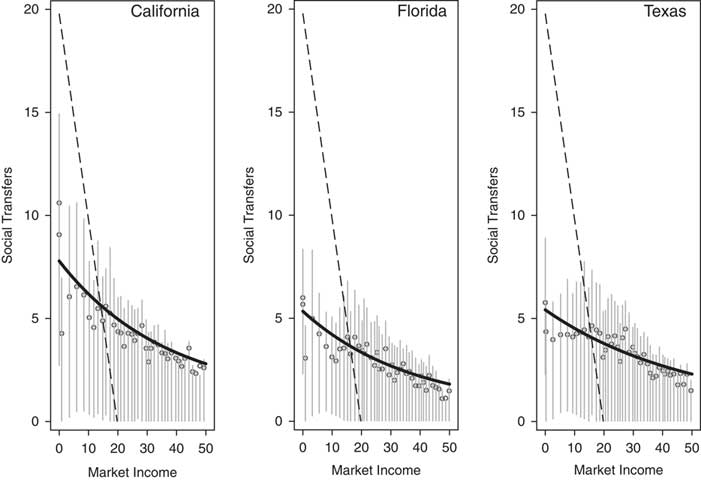
In fact, that the negative curvilinear relationship between social transfers and market income observed in Figure 1 is quite general (see Appendix B and Jusko 2008). We see similar relationships in Figure 2, for example, which reports the relationships between social transfers and market earnings in California, Florida, and Texas. In each panel, each data point represents 1 percent of the 2010–2014 pooled state sample; the vertical lines denote the interquartile range of social transfers for each group.Footnote ⁹ The diagonal, dashed line in each panel reports the amount of income needed at each income level to meet the poverty threshold; here, the 2014 official US poverty line (for a family of four, used here for consistency with later analysis), of $19,790.

Fig. 2

Social transfers, by market earnings, and States (2010–2014) Note: Figure 2 reports the relationship between social transfers by type and market income for California, New York, and Texas (2010–2014). Each data point represents 1 percent of the pooled 2010–2014 sample; error bars report the interquartile distribution at each income level. All currency amounts are reported in thousands of 2016 US dollars. The solid line reports predicted values for Equation 2. The dashed line reports predicted values for Equation 3.

There are, however, important differences in the relationships between social transfers and market income for these states: California provides generally higher levels of baseline relief to those with no market income (almost $7000) than does Florida or Texas (less than $5000). Second, the rate at which benefits decline is slightly lower in Texas than in the other two states. (Compare, e.g., where the curved line intersects the dashed line.) Finally, although we will not consider these differences extensively here, notice that the states differ in levels of support provided to those with relatively high incomes, at the right side of each panel. (This, of course, is not surprising: most of the income support received by those in households earning more than 20,000 is provided through social insurance programs, often administered by the states. In later analysis, we will use state unemployment benefits to validate our overall measure of poverty relief.)

Note that the solid lines in Figure 2 fit the relationships between market income and social transfers quite well for each state, and report predicted values from the following non-linear expression:

(2) $$ST_{{ij}}\, {\equals}\,\alpha _{j} {\plus}\beta _{{1j}} \rm exp(\beta _{{2j}} MI_{{ij}} ){\plus}e_{{ij}} .$$

Here, ST _ij denotes social transfer amounts and MI _i j denotes market income for individuals i=1 … n in states j=1 … J. The parameters α _j >0, β _1j >0, and β _2j <0 describe the bivariate relationship within each state and e _ij is a stochastic residual term.Footnote ¹⁰ As suggested above, the dashed line in Figure 2,

(3) $$ST_{{ij}} \,{\equals}\,\psi \,{\minus}\,MI_{{ij}} ,$$

reports the amount of income support needed so that all households have incomes at least equal to the poverty threshold, ψ, and will be important to our later analysis.

One important advantage of using Equation 2 to characterize the relationship between market income and social transfers is that the parameters have accessible, substantive interpretations. Notice, when β _2j <0,Footnote ¹¹ individuals who have no market income receive social transfers in the amount of α _j +β _1j —our measure of “baseline relief.” Similarly, for very high levels of MI _ij , ST _ij is expected to take on the value α _j . In the United States, this level corresponds to average social insurance benefits; outside the United States, this amount might include universal, non-means-tested non-contributory benefits like Germany’s universal allowance for families with children, Kindergeld. Finally, the expression β _1j (1−exp(β _2j )) can be used to estimate the rate at which benefit levels decline, with increased market earnings or the amount income support decreases with an increase from no market earnings to $1000. The parameters α _j , β _1j , and β _2j , therefore, jointly describe income support provided through a specific state’s safety net programs, and can be used as the basis for a comparison of poverty relief within a society over time, or across societies more generally.

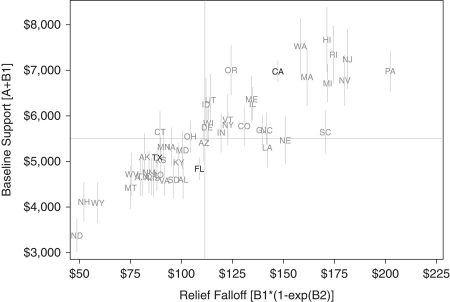
Figure 3 plots these estimates of baseline relief (α _j +β _1j ) against relief falloff (β _1j (1−exp(β _2j )) for pooled 2010–2014 state samples. The vertical axis reports the average amount of support provided to those with no market earnings, in each state. The horizontal axis reports estimates relief falloff—specifically, the increasing difference in the amount of benefits received by households with no earnings, and households with $1000 in earnings. For example, California households earning $1000 can expect $150 less in income support than households with no market income. Notice that, as observed above, although Texas provides considerably less baseline relief, the amount of relief falloff is also low, relative to California.Footnote ¹²

Fig. 3

Baseline relief and relief falloff, by State (2010–2014) Note: Figure 3 plots estimates of baseline relief (vertical axis)—α _j +β _1j —against relief falloff (horizontal axis)—β _1j ×(1−exp(β _2j )—for the US states, for pooled 2010–2014 state samples. Parameters are estimated for Equation 2. All currency amounts are reported in 2016 US dollars, for households. The solid lines report median values on each dimensions (2). Error bars report 95 percent confidence intervals.

The relationship between baseline relief and relief falloff, therefore, can be used to classify safety net programs: those states in the upper left quadrant, such as Connecticut, provide relatively high levels of baseline support, with comparatively low rates of relief falloff. Those state in the upper right quadrant, such as California and Washington, also provide high levels of baseline relief, but the rate at which benefits decline is quite high. States in the lower quadrants provide more limited baseline relief, but those on the right (e.g., Louisiana) have relatively high relief falloff, compared to those in the lower left quadrant (e.g., Texas).

Of course, a cross-state or time series comparison based on only one of the dimensions in Figure 3 would be an incomplete and potentially misleading measure of poverty relief in the United States. There are many examples of states with similar levels of baseline relief, for example, but quite different rates of relief falloff.Footnote ¹³ Nevertheless, we can use the relationship between market income and social transfers to develop a summary measure of poverty relief. The dashed line in Figure 2, Equation 3, reports the amount of income support that would bring all low-income families up to a poverty threshold, ψ.Footnote ¹⁴ Then, the ratio of the area under the curve defined by the observed relationship between market income and social transfers (Equation 2) to the triangular area defined by Equation 3 estimates of the amount of income support provided, relative to the total amount that would give all low-income households sufficient income to meet basic needs.Footnote ¹⁵ The poverty relief ratio $\scr R$ , then, can be estimated according to the following expression:

(4) $${\scr R}\,{\equals}\,{{{\int}_0^\tau (\alpha {\plus}\beta _{1} \cdot {\rm exp}(\beta _{2} \cdot {MI}))\partial {MI}{\plus}{\int}_\tau ^\psi (\psi {\minus}{MI})\partial {MI}} \over {{\int}_0^\psi (\psi \,{\minus}\,{MI})\partial {MI}}}.$$

Here, τ reports the point of intersection for Equations 2 and 3.Footnote ¹⁶ After integrating over the region of 0 to ψ, the poverty relief ratio $\scr R$ increases with baseline relief and as relief falloff decreases. Specifically

(5) $${{\partial \scr R} \over {\partial \alpha }},\,{{\partial \scr R} \over {\partial \beta _{1} }}{\rm ,}\,{\rm and}\,{{\partial \scr R} \over {\partial \beta _{2} }}\,\gt\,0.$$

Thus, for fixed ψ, the poverty relief ratio $\scr R$ provides a useful summary of safety net program support, with a meaningful substantive interpretation: $\scr R$ reports the average percentage of income support received by low-income households, of the support needed to have a total income equal to a specified poverty threshold.Footnote ¹⁷

To see how the poverty relief ratio is different from more standard poverty rate and poverty gap measures, compare Equation 1 to Equation 4. Foster, Greer and Thorbecke (Reference Foster, Greer and Thorbecke2010) recall the following example, given by Morduch (Reference Morduch1999, 99), that helpfully demonstrates an important difference between the poverty relief ratio and more commonly used FGT measures: suppose that a social program is able to target only relatively well-off low-income households (but not sufficiently to increase their incomes above the poverty line), while another provides benefits (in the same amount) to the very poor. Note that the poverty rate measure, P ₀, would be unable to distinguish between these policies: the number of low-income households remains unchanged. Further, the poverty gap measure (P ₁) would report that the policies are equally effective. (Only for γ>1 would differences in the implications of the policy be apparent.) Calculating the poverty relief ratio, however, draws attention to the important differences in the distribution of benefits: in the first case, the rate of relief falloff would likely be reduced. The second case would likely generate higher estimates of baseline relief. (The second program would be located higher on both dimensions presented in Figure 3.) Overall levels of poverty relief are also likely to be higher in the second case.

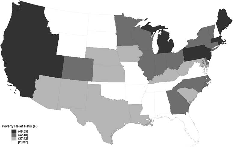
Figure 4 reports estimates of the poverty relief ratio for each state, with states grouped by quartile. (Appendix C reports estimates of the parameters α, β ₁, β ₂, and τ for each state, as well as estimates of the poverty relief ratio, $\scr R$ ; ψ is fixed at $19,790, the 2014 official poverty line.) On average, states provide about 46 percent of the poverty relief needed during this period, with some evidence of regional variation. Western states are over-represented in the highest quartile; all but two Southern states provided below-the-median levels of poverty relief.

Fig. 4

Poverty relief, by State (2010–2014) Note: Figure 4 reports estimates of the poverty relief ratio for each state, with states grouped by quartile. See the Appendices for estimation details.

Notice additionally that the poverty relief ratio $\scr R$ essentially orders the states as they appear in Figure 3, but distinguishes between states that offer similar levels of baseline benefits and have different levels of relief falloff. For example, in Figure 3, Connecticut and Louisiana provide approximately equal levels of baseline relief (about the median level), but rates of relief falloff are quite different in these states. Estimates of $\scr R$ take these differences into account and report higher values for those states (i.e., in this case, Connecticut) with lower rates of relief falloff. As Appendix C reports, average levels of poverty relief are estimated to be about 44 percent of the federal poverty line in Connecticut and 39 percent in Louisiana, a difference that represents about 23 percent of the entire range of $R$ values. Therefore, $\scr R$ provides an effective summary statistic for two key dimensions of safety net programs, baseline relief and relief falloff, and a substantively meaningful estimate of poverty relief in each state.

THE POVERTY RELIEF RATIO AND POLICY

Does $\scr R$ report meaningful differences (or changes) in safety net policy? If $\scr R$ is a valid measure of antipoverty relief, there should be some evidence of a positive relationship between our poverty relief ratio, $\scr R$ , and more generous safety net policy intentions. However, because $\scr R$ captures the multidimensionality of income support for low-income households, it likely correlates imperfectly with any given measure of policy.

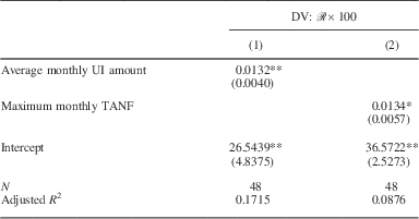
In fact, the evidence suggests that $\scr R$ is positively correlated with both state average unemployment benefits and with maximum TANF benefits. For example, those states that report the highest levels of unemployment benefits typically are in the highest quartile of the $\scr R$ distribution. Similarly, not surprisingly, states with relatively high maximum TANF benefit levels are typically associated with high estimates of poverty relief, although there is more variance in this bivariate relationship (Table 2).

Table 2

Poverty Relief and Policy (2010–2014)

Note: This Table reports ordinary least squares regression estimates of the relationship between poverty relief $\left( {\scr R{\times}}100} \right)$ and average monthly unemployment insurance (UI) and maximum Temporary Assistance to Needy Families (TANF) benefits.

Standard errors are reported in parentheses; **p<0.01, *p<0.05.

Sources: UI: Monthly Program and Financial Data: Summary Data for State Programs, by State (2010–2014); TANF: Welfare Rules Database (2010–2014).

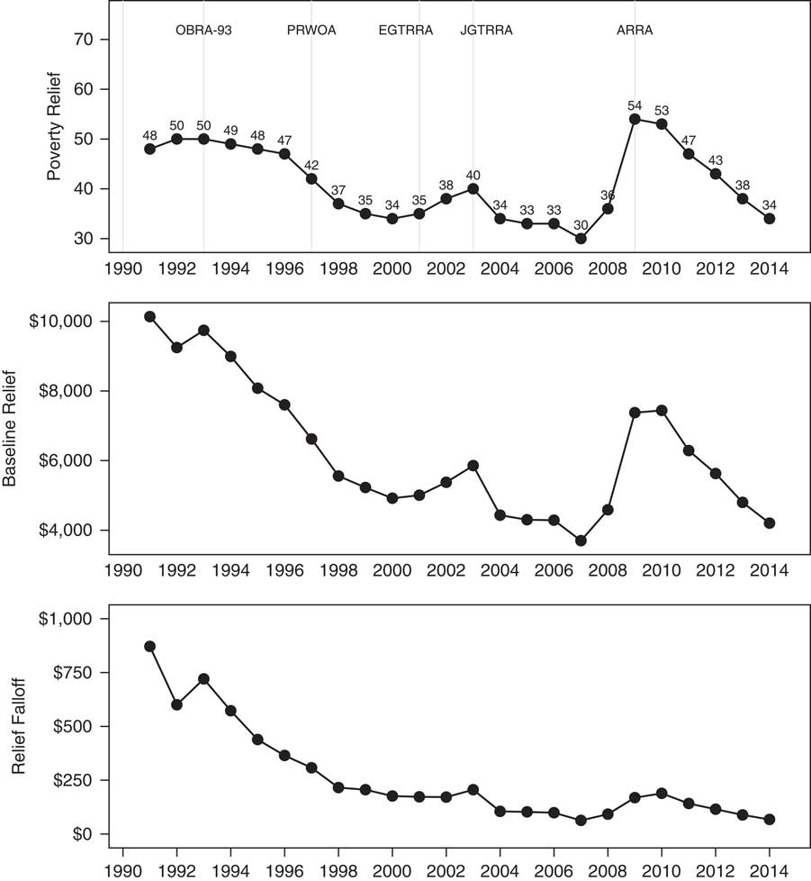
Finally, while a full evaluation of changes in American social policy is beyond the scope of this analysis, the fact that national estimates for $\scr R$ track major policy changes provides further evidence of the validity of our measure: Figure 5 reports estimates of the poverty relief ratio (top panel), baseline relief (middle panel), and relief falloff (bottom panel) for the United States from 1991 to 2014. At the end of this time series, only about 34 percent of the relief needed to bring an average low-income household’s income to the official poverty line is provided. While important shifts in safety net policy have changed levels of income support over this period, we observe a steady erosion of benefits following the Clinton-era welfare reform, with brief interruptions in the early 2000s and following the 2008 financial crisis. The middle panel demonstrates that most of this erosion comes from a dramatic decline in baseline relief—that is, support for those in deep poverty. The decline and leveling of relief falloff (seen in the bottom panel) reflects the expansion of EITC and increase in support for low-income working families.

Fig. 5

National poverty relief (1991–2014) Note: Figure 5 plots national estimates of the poverty relief ratio, baseline relief, and relief falloff for the 1991–2014 period.

Importantly, each major shift in policy corresponds to expected changes in $\scr R$ . For example, the initial increase in poverty relief observed in the top panel resulted from the Bush and Clinton administrations’ expansions of EITC (instituted by the Omnibus Budget Reconciliation Acts of 1990 and 1993), which dramatically decreased rates of relief falloff, observed in the bottom panel. Then, following the implementation of mid-1990s major welfare reform (PRWOA), we observe a significant decrease in baseline relief and a corresponding decline in overall poverty relief. Although we observe some safety net expansion following the Bush administration’s post-9/11 economic stimulus, levels of poverty relief remained steady until the major expansion implemented by President Obama in the American Recovery and Reinvestment Act of 2009, which temporarily expanded federal unemployment benefits as well as near-cash food and energy benefits.

Earlier, we suggested that $\scr R$ , compared to more standard threshold-based measures, has the advantage of generally preserving the rank order of observations across different poverty thresholds (here, values of ψ). This feature significantly allows the effects of policy to be examined in a consistent and reliable way. Before considering the implications of this analysis, here, we briefly demonstrate how, with other threshold-based measures, rank order varies with the poverty threshold, and how this might affect understanding of the impact of various policy measures.

The right panel of Figure 6 plots estimates of $\scr R$ for each state against estimates using 50, 150, and 200 percent of the official poverty line, against estimates generated using the original poverty threshold. For comparison, the left and middle panels of Figure 6 repeats this analysis, with the same data, but using the more common proportional reduction in poverty rate and gap measures (the most commonly used measures of social policy outcomes). The advantage of $\scr R$ over the poverty rate and gap measures is especially clear when comparing the relative ranking of North Dakota for each measure and threshold: when the effectiveness of safety net programs is measured using the poverty reduction rate measure, North Dakota ranks second, second, tenth, and fourth, for thresholds equal to 50, 100, 150, and 200 percent of the official poverty line, respectively, and tenth, third, fifth, and second, for the poverty gap measures, when states are ranked in order of increasingly effective programs. Regardless of threshold, however, North Dakota always ranks first (i.e., least effective) when $\scr R$ is used instead. More generally, Spearman’s rank-order correlation coefficients range from 0.38 to 0.52 for the poverty reduction rate measures estimated using different thresholds. Rankings using the poverty gap measure are more stable, with Spearman’s rank-order correlation coefficients ranging from 0.58 to 0.79, but still less than similar coefficients estimated for $\scr R$ , which exceed 0.96 across all of the various thresholds.

Fig. 6

Rank order with varying poverty thresholds Note: Figure 6 compares proportional reduction in poverty rate and gap estimates calculated for different poverty thresholds (50, 150, and 200 percent of the official poverty line), against estimates of $R$ calculated for the same thresholds.

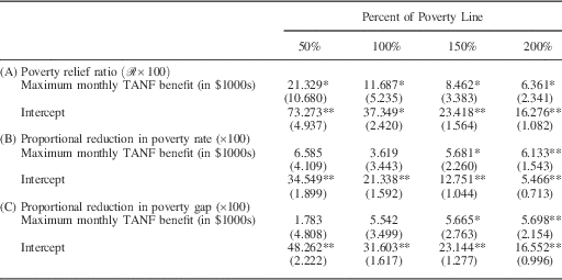
Table 3 demonstrates the importance of rank-order stability with a simple example, reporting the estimated relationship between the poverty relief ratio, proportional reduction in the poverty rates and gaps, and maximum TANF benefits. We might reasonably expect that, as a proximate measure of the generosity of transfers in each state, maximum TANF benefits will be strongly and consistently related to levels of poverty relief overall. In fact, this is the case when the poverty relief ratio is used as a measure of the effectiveness of anti-poverty policy. However, when alternate threshold-based measures of poverty reduction are used, instead, this expected relationship is estimated with considerably more variance than conventionally accepted, and would likely result in conflicting substantive conclusions. (Notice, e.g., that when the official poverty line is used, the generosity of TANF benefits has an ambiguous effect on the reduction of poverty rates or gaps.) In this case, if the effectiveness of anti-poverty policy is evaluated using existing measurement strategies, conclusions about whether TANF benefit amounts matter will depend on which poverty threshold is used.

Table 3

Regression Analysis Using Different Poverty Thresholds

Note: This Table reports the results of a simple experiment in which several versions of the poverty relief ratio and the proportional reduction in poverty rates and gaps, estimated using several poverty thresholds, are regressed on maximum monthly Temporary Assistance to Needy Families (TANF) benefits.

**p<0.01; *p<0.05.

IMPLICATIONS

In this discussion, we have presented a measure of poverty relief that offers several important advantages over standard measures used in the literature. Specifically, this measure uses a total income approach, which readily accommodates the portfolios of support on which low-income households rely. In combination with a poverty threshold, we have shown that the parameters that describe the relationship between market income and social transfers provide a useful way to distinguish social policy and can be used to generate a ratio estimate of the proportion of income support provided, relative to the account of support needed to raise all poor families’ incomes to a specified threshold. Thus, the poverty relief ratio incorporates explicit policy goals.

We anticipate three sets of concerns about the general utility of $\scr R$ :

First, some readers may question the utility of a parameterized model of poverty relief. Because the model generally fits the data well and can be easily estimated, we believe that there is little information lost through its estimation. Further, the values that the parameters α, β ₁, and β ₂ take provide important, substantively meaningful insight into the nature of poverty relief and can be used as the basis of comparative analysis. As suggested above, the non-linear set-up used here can easily accommodate a hierarchical model, in which levels of baseline relief or relief falloff are predicted by political and economic characteristics of each state.

Second, other readers may contend that $\scr R$ provides no information about the rate of poverty. This is undoubtedly true: we focus instead on levels of income support and the distribution of benefits among low-income households.

Finally, like other measures of safety net program effectiveness relying on individual-level surveys (i.e., the distributional and poverty reduction rate measures), $\scr R$ is susceptible to bias introduced by under-reporting of benefits and limited by available survey measures. To the extent that especially those with no market income understate the amount of support they receive, $\scr R$ may under-estimate levels of poverty relief. Wheaton (Reference Wheaton2007) suggests that CPS data may be especially problematic, although other income and labor force surveys also underreport safety net program participation. To provide some confidence in the substantive interpretation of the results presented here, a time series analysis evaluated national trends in poverty relief using Survey of Income and Program Participation data. While there are some differences in the annual estimates of $\scr R$ , for example, they are very small, and the bias introduced by the under-reporting of benefits does not complicate the substantive interpretation of the overtime analyses presented here. Readers may also be interested in the relative relief provided by federal and state programs; to the extent that surveys measure support for different programs, the poverty relief measure can facilitate this sort of analysis.

This paper has presented a new measure of poverty relief and its component parameters that provide a new way to characterize and evaluate safety net programs in the United States (and abroad). Here, we find substantial cross-state variation in the effectiveness of safety net programs: Some states, such as Alabama and Wyoming, provide only about a third of the income support needed to raise incomes to the poverty threshold. Other states, including Washington and Massachusetts provide about 50 percent. While most of the cross-state variation in poverty relief is attributable to differences in baseline relief (a bivariate regression generates estimates of R ²=0.98), $\scr R$ usefully distinguishes between states with different rates of relief falloff. In tracking federal policy from 1991 to 2014, we find that even at its most expansive level, the American safety net provided only about half of the support required to meet basic needs. The declining levels of support to those with no market income (our baseline relief) is especially concerning. To the extent that the official poverty line underestimates the amount needed, and because our estimates here includes near-cash transfers, as well as cash transfers, this analysis presents a particularly dire impression of the American social safety net.

What sets this analysis apart from existing work, importantly, is a strategy for evaluating the effectiveness of different anti-poverty policies, in a way that is invariant to how poverty is defined. The poverty relief ratio, therefore, provides both a reliable means of examining the impact of different policies, as well as a measurement that can be used for comparison across quite different systems.