


1 Introduction
Dynamical systems provide a mathematical framework for describing how a state evolves under repeated application of a rule. Two recurring themes in this theory are complexity and chaotic behavior. One way to quantify complexity is through entropy, which measures the exponential growth rate of distinguishable orbit patterns. Another approach is to describe chaos via the existence of large scrambled sets, as in Li–Yorke chaos. These notions are closely related in many classical settings, and understanding their relationship in structured symbolic systems is a central topic in topological dynamics.
In this paper, we study these themes in a class of symbolic systems built from monoid actions on trees. More precisely, we consider Markov-type constraints on labelings of a tree determined by an adjacency matrix, leading to the notion of a Markov tree-shift. Our first goal is to characterize several standard mixing properties for these systems. Our second goal is to compute their entropy via an explicit formula. As a third goal, we introduce a strengthened, structure-sensitive form of Li–Yorke chaos, which we call locally Li–Yorke chaos (see Section 1.3). The main result in this direction shows that, in our setting, positive entropy is equivalent to locally Li–Yorke chaos.
Let
$\Sigma $
 be a finite alphabet, M be a 0–1 matrix indexed by
$\Sigma $
 , and
$\Sigma _M$
 be the subshift of finite type on
$\mathbb {N}$
 with adjacency matrix M. Denote by
$\rho _M$
 the spectral radius of the matrix M. For
$n\geq 0$
 ,
$\Sigma _M^n$
 is the set of words (in
$\Sigma _M$
 ) of length n so that
$\Sigma _M^1 = \Sigma $
 and
$\Sigma _M^0 = \{\epsilon \}$
 , where
$\epsilon $
 stands for the empty word. Then,
$\Sigma _M^* = \bigcup _{n=0}^\infty \Sigma _M^n$
 is a monoid equipped with a binary operation
$\bullet :\Sigma _M^*\times \Sigma _M^* \to \Sigma _M^*$
 by

where
$u=i_1\cdots i_n\in \Sigma _M^n, v=j_1\cdots j_m\in \Sigma _M^m$
 and
$n,m\geq 1$
 , and
$\epsilon \bullet w=w$
 and
$w\bullet \epsilon =w$
 for all
$w\in \Sigma _M^* $
 . We write
$|v| = n$
 for
$v \in \Sigma ^n$
 so that
$|v|$
 is the length of the word v.
The set
$\Sigma _M^*$
 also has the structure of a countable tree, with
$v \preceq w$
 if and only if there exists u such that
$vu = w$
 with
$v \prec w$
 if
$v\bullet u \neq v$
 and so
$v \neq w$
 . For
$w \in \Sigma _M^*$
 , the set
$[w] = \{v : v \preceq w\}$
 is the set of all predecessors of w together with w itself. For
$v \in \Sigma _M^*$
 , the set
$(v\Sigma = \{vi : i \in \Sigma \})\setminus \{v\}$
 is the set of immediate successors of v. Thus,
$[\epsilon ] = \{\epsilon \}$
 and
$[i] = \{\epsilon , i\}$
 for
$i \in \Sigma $
 . If
$v = i_1 \cdots i_n \in \Sigma _M^n$
 , then the listing of the points of
$[v]$
 in order is the sequence
$\{\epsilon , i_1, i_1i_2, \ldots , i_1i_2 \ldots i_n\}$
 so that
$[v]$
 has cardinality
$n+1$
 . Thus, the listing for v is the unique sequence
$\{v_0, v_1, \ldots , v_n\}$
 in
$\Sigma _M^*$
 such that
$v_0 = \epsilon $
 ,
$v_n = v$
 , and
$v_i$
 is an immediate successor of
$v_{i-1}$
 for
$i = 1, \ldots , n$
 .
A subtree is a nonempty subset K of
$\Sigma _M^*$
 such that
$w \in K$
 implies
$[w] \subseteq K$
 . That is, a subtree K contains the predecessors of any element of K. In particular,
$\epsilon \in K$
 for any subtree K. Clearly,
$[w]$
 is the smallest subtree that contains w. The union and the intersection of any family of subtrees are each of the subtrees. For a subtree K, we define the boundary

That is,
$\partial K$
 consists of the elements of K that are maximal with respect to the partial order
$\preceq $
 . If a subtree is finite, then
$\partial K$
 is nonempty. For example,
$\Sigma _M^{\leq n} = \bigcup _{k=0}^n \Sigma _M^k$
 is a subtree with
$\partial \Sigma _M^{\leq n} = \Sigma _M^n$
 .
Assume that K and
$K_1$
 are subtrees and that
$v \in K$
 satisfies

That is, if
$i \in K_1$
 , then the successor
$vi$
 of v does not lie in K. For example, it suffices that
$v \in \partial K$
 since in that case,
$\{i \in \Sigma : vi \in K\} = \emptyset $
 . We then define the attachment of
$K_1$
 to K at v to be

with
$K \cap \{vw : w \in K_1\} = \{v\}$
 . Note that the intersection condition follows from (1-1). Clearly, for
$w \in K$
 ,
$[w] \subseteq K \subseteq K \oplus _v K_1$
 and for
$w \in K_1$
 ,
$[vw]=[v] \cup \{vu : u \in [w]\} \subseteq K \oplus _v K_1$
 . Thus,
$K \oplus _v K_1$
 is a subtree. In particular, if
$i \in \Sigma $
 and for
$v \in K$
 we have
$vi \notin K$
 , then we write
$K \oplus _v i$
 for
$K \oplus _v [i]$
 . That is,

We denote
$vK=\{vw : w\in K\}$
 for
$v\in \Sigma _M^*$
 and K a subtree. In particular, if
${K=\{\epsilon \}\cup \Sigma _M}$
 , then
$vK\setminus \{v\}$
 is the set of immediate successors of v. We now introduce types of subtrees of
$\Sigma _M^*$
 . For
$v\in \Sigma _M^*$
 , the follower set
$F_{\Sigma _M^*}(v)$
 of v in
$\Sigma _M^*$
 is defined as

It is straightforward to check that
$F_{\Sigma _M^*}(v)$
 is a subset of
$\Sigma _M^*$
 . Hence,
$F_{\Sigma _M^*}(v)$
 is a subtree. Note that
$\Sigma _M^*$
 can be represented as

where
$\sqcup $
 means disjoint union.
A relation R on a finite set of labels A is a subset of
$A \times A$
 with

We write
$R(a) = \{b \in A : (a, b) \in R\}$
 . Call the relation proper when
${R(a) \neq \emptyset }$
 for all
$a \in A$
 . The relation is surjective when R and
$R^{-1}$
 are both proper.
With A a finite set of labels, the full tree-shift is the action of the monoid
$\Sigma _M^*$
 on the space
$A^{\Sigma _M^*}$
 . That is,
$(tv)(w) = t(vw)$
 for all
$vw\in \Sigma _M^*$
 . In general, a tree-shift is the restriction of the action to a nonempty, closed subset of
$A^{\Sigma _M^*}$
 . To define a Markov tree-shift, we begin with an indexed family
$\mathcal {R} = \{R_i : i \in \Sigma \}$
 of proper relations on A and we let
$R = \bigcup _i R_i$
 so that

For K a subtree of
$\Sigma _M^*$
 , we define
$T_K$
 to be the closed subset of
$A^K$
 given by

We write T for
$T_{\Sigma _M^*}$
 . Thus,

That is,

If
$R_i=R_j$
 for all
$i,j \in \Sigma $
 , then T is called a hom Markov tree-shift.
It should be noted that the action of the monoid
$\mathbb {Z}^{d}$
 on a closed subset of
$A^{\mathbb {Z}^{d}}$
 with family of proper relations
$\mathcal {R}=\{R_i: 1\leq i \leq d\}$
 (also called Markov shift [Reference Lind and Marcus26]) is

where
$e_i$
 is the i th standard basis vector of
$\mathbb {Z}^d$
 . Markov shifts X are commonly used in statistical physics to model a variety of physical systems, for example, the hard-square model [Reference Baxter, Enting and Tsang10] and Ice model [Reference Lieb24]. The Markov tree-shift [Reference Aubrun and Béal1–Reference Ban and Chang3, Reference Petersen and Salama30, Reference Petersen and Salama31] has received increasingly more attention in recent times because of its intriguing dynamics and distinct phenomena from X [Reference Ban, Chang, Hu, Lai and Wu4, Reference Ban, Chang, Hu and Wu6]. The following three topics are the main purpose of this paper.
1.1 Mixing properties
The topological mixing properties are global features of a dynamical system [Reference Blanchard11]. They aim to understand how complicated a topological dynamical system could be, such as, irreducible (or topological transitive), totally transitive, topological mixing, block bluing, and strongly irreducible. We refer the reader to [Reference Foryś, Huang, Li and Oprocha13, Reference Huang, Li, Ye and Zhou19] for further developments. The formal definitions of mixing properties are given as follows. Let T be a Markov tree-shift. We define a metric
$d': \Sigma _M^*\times \Sigma _M^* \to [0,\infty )$
 by
$d'(u, v) = |[u]\setminus [v]|+|[v]\setminus [u]|$
 for all
$u,v \in \Sigma _M^*$
 . We denote the distance between two finite subsets
$F_1, F_2\subseteq \Sigma _M^*$
 by
$d(F_1, F_2)=\min _{u\in F_1,v\in F_2}d'(u, v)$
 . For any
$i,j\in \Sigma $
 , if
$ivj\in \Sigma _M^*$
 for some v with
$i\neq iv$
 and
$v\neq vj$
 , then we call T:
-
• irreducible (IR) if for any $h_1\in T_{K_{i,n}}$
 and
$h_2 \in T_{K_{j,m}}$
, there exist
$t \in T$
and
$w j \in F_{\Sigma _M^*}(i)$
with
$wj\neq w$
and
$|wj|\geq n$
such that
$t|_{K_{i,n}} =h_1$
and
$t|_{wjK_{j,m}} = h_2$
, where
${K_{i,n}=F_{\Sigma _M^*}(i)\cap \Sigma _M^{\leq n}}$
;
-
• totally transitive (TT) if for any $wj \in F_{\Sigma _M^*}(i)$
with
$wj\neq w$
and
$w\neq ww$
, there exist
$t \in T$
and
$N \in \mathbb {N}$
such that
$t|_{K_{i,n}} = h_1$
and
$t|_{w^NjK_{j,m} } = h_2$
; -
• topological mixing (TM) if for any finite subtrees $K_1 \subseteq F_{\Sigma _M^*}(i)$
and
$K_2 \subseteq F_{\Sigma _M^*}(j)$
, there exists
$N \in \mathbb {N}$
such that for any
$h_1\in T_{K_1}$
,
$h_2\in T_{K_2}$
, and
$wj\in F_{\Sigma _M^*}(i)$
with
$d(K_1, \{wj\})\geq N$
and
$w\neq wj$
, there exists
$t\in T$
such that
$t|_{K_1}=h_1$
and
$t|_{wjK_2}=h_2$
; -
• block gluing (BG) if there exists $N \in \mathbb {N}$
such that for any
$h_1\in T_{K_{i,n}}$
,
$h_2\in T_{K_{j,m}}$
, and
$wj \in F_{\Sigma _M^*}(i)$
with
$d(K_{i,n},\{wj\})\geq N$
and
$w \neq wj $
, there exists
$t \in T$
such that
$t|_{K_{i,n}} = h_1$
and
$t|_{wjK_{j,m}} = h_2$
; -
• strongly irreducible (SI) if there exists $N \in \mathbb {N}$
such that for any
$h_1\in T_{K_1}$
,
$h_2 \in T_{K_2}$
, and
$wj \in F_{\Sigma _M^*}(i)$
with
$d(K_1, \{wj\}) \geq N$
and
$w \neq wj$
, there exists
$t \in T$
such that
${t|_{K_1} = h_1}$
and
$t|_{wjK_2} = h_2$
.


Note that
$\text {SI}\Rightarrow \text {BG}\Rightarrow \text {TM}\Rightarrow \text {TT}\Rightarrow \text {IR}$
 .
Let
$\mathcal {R}=\{R_i: i\in \Sigma \}$
 be the family of proper relations corresponding to T. In fact, each relation
$R_i$
 can be written as an
$|A|\times |A|\, 0$
 –
$1$
 matrix
$A_i$
 defined by

We note that
$R_i$
 is a proper (respectively surjective) relation if and only if the row (respectively row and column) sums of
$A_i$
 are positive. For
$u=i_1\cdots i_n \in \Sigma _M^n$
 , denote
$A_{i_1}\cdots A_{i_n}$
 by
$A_u$
 .
We say T satisfies property:
-
(H1) if for all $a,b\in A$
and
$i,j\in \Sigma $
, whenever there exists
$v\in \Sigma _M^*$
such that
${vj\in F_{\Sigma _M^*}(i)}$
and
$v\neq vj$
, there exists
$u\in \Sigma _M^*$
with
$uj\in F_{\Sigma _M^*}(i)$
and
$u\neq uj$
such that
${(A_{uj})_{a,b}>0}$
; -
(H2) if $A_u$
is irreducible for all
$u \in \Sigma _M^*$
with
$u\neq uu$
; -
(H3) if there exists $N\in \mathbb {N}$
such that
$A_u$
is positive for all
$u\in \Sigma _M^*$
with
$|u|\geq N$
.


The first main result of this paper is given as follows.
Theorem 1.1. Let T be a Markov tree-shift. Then:
-
(1) T is IR $\iff \, T$
satisfies Property (H1); -
(2) T is TT $\iff \, T$
satisfies Property (H2); -
(3) T is SI $\iff \, T$
satisfies Property (H3).


In particular, if
$\rho _M=1$
 , then T is TT if and only if T is SI.
Remark 1.2. In general, T being IR does not necessarily imply that it is TT (even when
$\rho _M=1$
 ). For instance, consider the case where
$M=\big [\!\begin {smallmatrix} 0 & 1 \\ 1 & 0 \end {smallmatrix}\!\big ]$
 , and the
$A_i= \big [\!\begin {smallmatrix} 0 & 1 \\ 1 & 0 \end {smallmatrix}\!\big ]$
 for all
$i\in \Sigma $
 . It can be verified that T is IR but not TT.
1.2 Entropy
Compared with the mixing properties, the entropy is a local feature of a dynamical system [Reference Blanchard11]. It is a fundamental concept in topological dynamics that measures the complexity of a dynamical system (or a maximal subsystem). It quantifies the rate of growth of distinguishable orbits over time, reflecting the system’s unpredictability and chaotic behavior. We refer the reader to [Reference Huang and Jin16, Reference Huang, Li and Ye18, Reference Huang, Li, Ye and Zhou19] for recent developments on related topics. The formal definition of entropy is given as follows. Let T be a Markov tree-shift. The entropy of T is defined by

We remark that the authors [Reference Petersen and Salama30] provide the existence of limit of (1-3) when M is a full one matrix, and this also exists for a larger class of M [Reference Ban, Chang, Wu and Wu7].
The second main result is given as follows.
Theorem 1.3. Let T be a Markov tree-shift with
$\rho _M=1$
 . If T is TT, then

where
$p_\ell $
 ,
$S_\ell $
 ,
$j_{\ell ,r}$
 for all
$1\leq \ell \leq m$
 ,
$1\leq r\leq \vert S_\ell \vert $
 are defined in Section 2, and
${M_\ell =A_{u_{\ell ;0,|S_\ell |}}}$
 , where
$u_{\ell ;0,|S_\ell |}$
 is defined in (3-12).
We remark that if the assumption that T is TT is removed, then the ‘
$=$
 ’ in (1-4) becomes ‘
$\leq $
 ’. Theorem 1.3 has some applications.
Corollary 1.4. Let
$\rho _M=1$
 . The following assertions hold true.
-
(1) If T is a hom Markov tree-shift with primitive $A_i$
, then
$h(T)=h(\Sigma _{A_i})$
. -
(2) The set of entropies of TT Markov tree-shifts is dense in $[0,\infty )$
. -
(3) If T and $T'$
are TT Markov tree-shifts with
$A_{i}\leq A^{\prime }_{i}$
for all
$i\in \Sigma $
and there exists an
$1\leq \ell \leq m$
such that
$p_\ell>0$
,
$M_\ell <M^{\prime }_\ell $
, and
$M^{\prime }_\ell $
is irreducible, then
$h(T)<h(T')$
. -
(4) If T is TT and there exists an $1\leq \ell \leq m$
such that
$p_\ell>0$
and
$\rho _{M_\ell }>1$
, then
${h(T)>0}$
.


Corollary 1.4(1) indicates that the entropy of a hom Markov tree-shift is equal to the entropy of a shift of finite type. This conclusion has been revealed in [Reference Ban, Chang, Hu, Lai and Wu5] and Corollary 1.4 offers a distinct approach. Corollary 1.4(2) indicates that the set of all possible values of
$h(T)$
 , where T is TT, is abundant. The characterization for the monotonicity of
$h(T)$
 is given by Corollary 1.4(3). Finally, Corollary 1.4(4) presents a sufficient condition for the positivity of
$h(T)$
 . For related topics, we refer the reader to [Reference Lind25, Reference Lind and Marcus26, Reference Pavlov28, Reference Quas and Trow33]. We conclude Theorem 1.3 by making some remarks. Explicit computation of the entropy in (1-2) is generally difficult, since only a few examples admit closed formulas [Reference Baxter8, Reference Baxter9]. However, the explicit computation of
$h(X)$
 is of particular importance [Reference Georgii14] in statistical physics. Consequently, a variety of approximation methods have been developed for studying entropies [Reference Marcus and Pavlov27–Reference Pavlov29]. The study of the dynamics or thermodynamics of the shift on countable graphs has been extensively researched for a long time [Reference Grigorchuk and Stepin15, Reference Preston32, Reference Zachary35] and it is worth noting that Theorem 1.3 provides an explicit entropy formula for a type of multidimensional shift. However, the exact number of the entropy for a Markov tree-shift with
$\rho _M>1$
 is still unknown. We hope our perspective sheds some new light on the calculation of the entropies for general T (or X). Finally, if
$M=[1]$
 , then
$\Sigma _M^*=\mathbb {N}$
 and (1-4) shows that
$h(T)=\log \rho _{A_1}$
 , which is the well-known entropy formula for the
$\Sigma _{A_1}$
 [Reference Lind and Marcus26].
1.3 Li–Yorke chaos
Li–Yorke chaos [Reference Li and Yroke23] provides a definition of chaos based on the existence of scrambled (or chaotic) sets, which describe how points in a dynamical system behave in an unpredictable and nonperiodic manner. Blanchard, Glasner, Kolyada, and Maass [Reference Blanchard, Glasner, Kolyada and Maass12] proved that positive entropy implies Li–Yorke chaos (we remark that the authors obtained this result using ergodic methods, and for a combinatorial proof, see [Reference Kerr and Li20]). Moreover, the result also holds for sofic group actions by Kerr and Li [Reference Kerr and Li21, Corollary 8.4]. In this subsection, types of Li–Yorke chaos are introduced and, as an application of Theorem 1.3, we obtain that positive entropy is equivalent to locally Li–Yorke chaos, which is stronger than traditional Li–Yorke chaos. We also refer the reader to [Reference Huang and Jin16, Reference Huang, Li and Ye17, Reference Li and Ye22] for recent studies of related topics. The formal definitions are given as follows. Let
$v\in \Sigma _M^*$
 and
$t\in T$
 . Recall that
$tv(w)=t(vw)$
 for all
$vw\in \Sigma _M^*$
 . In particular, if
$M=[1]$
 , then
$tv(w)=t(v+w)$
 (for all
$v+w\in \mathbb {Z}$
 ) is the
$\mathbb {Z}$
 -action acting on
$\Sigma _{A_1}$
 . Let K be a subtree and
$h_1, h_2\in T_K$
 . The distance between
$h_1$
 and
$h_2$
 is a function
$f: T_K\times T_K \to [0,\infty )$
 defined as

A subset
$S\subseteq T$
 is called a chaotic set in the sense of Li–Yorke for
$\{v\}$
 if for any
$t_1, t_2 \in S$
 with
$t_1\neq t_2$
 ,

We say T is Li–Yorke chaotic (LY) if T contains an uncountable chaotic subset. An infinite subtree of the form
$\{\epsilon , i_1, i_1i_2, \ldots \}$
 is called a path in
$\Sigma _M^*$
 . Let
$S_1,\ldots ,S_m$
 be sinks in M and
$I_{S_\ell }\subseteq \Sigma $
 be the set of indices of
$S_\ell $
 . We say a path
$p=\{\epsilon , i_1, i_1i_2, \ldots \}$
 is in
$S_\ell $
 if there exists
$k\in \mathbb {N}$
 such that
$i_k\in I_{S_\ell }$
 . We say T is weakly Li–Yorke chaotic (WLY) if there exists a path p such that
$T_p$
 contains an uncountable chaotic subset. We say T is strongly Li–Yorke chaotic (SLY) if for any path p,
$T_p$
 contains an uncountable chaotic subset. We say T is locally Li–Yorke chaotic (LLY) if there exists
$1\leq \ell \leq m$
 with
$p_\ell>0$
 such that every path
$p\in S_\ell $
 satisfies that
$T_p$
 contains an uncountable chaotic subset. Note that SLY
$\Rightarrow $
 LLY
$\Rightarrow $
 WLY. However, the following example shows that the converse does not hold in general.
Example 1.5. Let
$A=\{a,b\}$
 ,
$\Sigma =\{1,2\}$
 , and

-
(1) If
$$ \begin{align*} A_1=\begin{bmatrix} 1 & 0\\ 0 & 1 \end{bmatrix} \quad\text{and}\quad A_2=\begin{bmatrix} 1 & 1\\ 1 & 1 \end{bmatrix}, \end{align*} $$then T is LLY but not SLY.
Indeed, M has exactly one sink, $S_1$
, with index set
$I_{S_1}=\{2\}$
, and hence,
$p_1=1$
. If p is a path that eventually enters
$S_1$
, then the labeling rule of
$A_2$
implies that
$T_p$
contains an uncountable chaotic set. Thus, T is LLY.However, if
$$ \begin{align*} p=\{\epsilon,1,11,\ldots\}, \end{align*} $$then $T_p=\{a^p,b^p\}$
, which is finite. Hence,
$T_p$
is not Li–Yorke chaotic, and therefore, T is not SLY.
-
(2) If
$$ \begin{align*} A_1=\begin{bmatrix} 1 & 1\\ 1 & 1 \end{bmatrix} \quad\text{and}\quad A_2=\begin{bmatrix} 1 & 0\\ 0 & 1 \end{bmatrix}, \end{align*} $$then T is WLY but not LLY.
If
$$ \begin{align*} p=\{\epsilon,1,11,\ldots\}, \end{align*} $$then $T_p=A^p$
, which contains an uncountable chaotic set. Hence, T is WLY.
However, if p is a path that eventually enters $S_1$
, then the labeling rule of
$A_2$
implies that every chaotic subset of
$T_p$
is finite. Therefore, T is not LLY.


The final main result is given as follows.
Theorem 1.6. Let T be a Markov tree shift with
$\rho _M=1$
 . Then:
-
(1) T is LLY $\Rightarrow $
T is LY; -
(2) if T is TT, then T is LLY if and only if $h(T)>0$
.


Remark 1.7. T being LY does not necessarily imply that it is LLY, as can be seen by considering the same setup as in Example 1.5(1).
Remark 1.8. The notion of locally Li–Yorke chaos introduced here relies essentially on the sink decomposition of the symbolic tree
$\Sigma _M^*$
 . In general dynamical systems
$(X,f)$
 , there is typically no canonical analogue of such a tree or path structure and, therefore, the present definition does not directly extend to arbitrary systems.
Conceptually, locally Li–Yorke chaos may be interpreted as Li–Yorke chaos occurring along distinguished invariant substructures with positive asymptotic weights. While the implication from positive entropy to Li–Yorke chaos is well understood in general settings (as discussed above), a systematic study of such a localized version of Li–Yorke chaos for general dynamical systems does not appear to have been developed so far. Extending this idea to broader classes of systems remains an interesting direction for future research.
The rest of this paper is organized as follows. In the next section, we introduce some notation that is beneficial for the proof of theorems. In Section 3, we provide the proofs of theorems. In Section 4, we give the flow of the proof of Theorem 1.3 through an example, and we obtain a Markov tree-shift T (T is not TT) where
$h(T)$
 is strictly less than the entropy formula in Theorem 1.3.
2 Preliminaries
In the following, we assume that all row and column sums of M are positive and let m be the number of sinks (submatrices of M) of M, say
$S_1,S_2,\ldots ,S_m$
 . For
$1\leq \ell \leq m$
 , let
$I_{S_\ell }$
 be the index set of
$S_\ell $
 and denote it by

where
$|S_\ell |$
 is the size of
$S_\ell $
 . Since
$\rho _M=1$
 , we may assume that
$S_\ell $
 is a cycle, that is,

and the other elements of
$S_\ell $
 are all
$0$
 .
For
$1\leq \ell \leq m$
 and
$1\leq k \leq n$
 , let

be the set of all words
$i_1i_2\cdots i_n\in \Sigma _M^n$
 , where the k th generator
$i_k$
 of the word is an element in
$I_{S_\ell }$
 and every generator before
$i_k$
 of this word is not in
$I_{S_\ell }$
 . Note that if
$i_1i_2\cdots i_n\in \Sigma _M^{n;k,\ell }$
 , since
$S_\ell $
 is a sink, we have
$i_r\in I_{S_\ell }$
 for all
$k\leq r\leq n$
 . Then, by
$S_\ell $
 being a cycle, we have that for
$k\geq 1$
 and
$1\leq \ell \leq m$
 , the cardinality
$|\Sigma _M^{n;k,\ell }|$
 of the set
$\Sigma _M^{n;k,\ell }$
 has the same quantity for all
$n\geq k$
 , and is obtained by

where
$M^0$
 is the
$d\times d$
 identity matrix. For
$1\leq r \leq |S_\ell |$
 , let

We observe that

Thus,
$|\Sigma _M^{n;k,\ell }|=\sum _{r=1}^{|S_\ell |}|\Sigma _M^{n;k,\ell ,r}|$
 .
For
$1\leq \ell \leq m$
 , define

if the limit exists. In fact, if the limit (2-4) exists, then the following limit exists:

and is equal to
$p_\ell $
 (see the proof of Theorem 1.3 for details). That is,
$p_\ell $
 is the probability of a vertex in
$\Sigma _M^*$
 belonging to
$\Sigma _M^{n;k,\ell }$
 for some n.
3 Proof of theorems
In this section, we prove Theorem 1.1 in Subsection 3.1, Theorem 1.3 in Subsection 3.2, and Theorem 1.6 in Subsection 3.3. The corresponding tools are provided in their respective subsections.
3.1 Proof of Theorem 1.1
In this subsection, we prove Theorem 1.1. The following lemma is needed before the proof.
Lemma 3.1. Let
$K_1,K_2\subseteq \Sigma _M^*$
 be finite subtrees,
$h_1\in T_{K_1}$
 and
$h_2\in T_{K_2}$
 . If
$K_2$
 attaches to
$K_1$
 at v and
$h_1(v)=h_2(\epsilon )$
 , then there exists
$h_3\in T_{K_1\oplus _v K_2}$
 such that
$h_3|_{K_1}=h_1$
 and
$h_3|_{vK_2}=h_2$
 .
Proof. It suffices to show this lemma in the case
$K_2 = [i] $
 , where
$i \in \Sigma $
 . Indeed, since
$(h_1(v),h_2(i))=(h_2(\epsilon ),h_2(i))\in R_i$
 , there exists
$h_3\in T_{K_1\oplus _v i}$
 such that
$h_3|_{K_1}=h_1$
 and
${h_3(vi)=h_2(i)}$
 . This implies
$h_3|_{vK_2}=h_2$
 .
Proof of Theorem 1.1.
(1) We claim that T is IR if and only if T satisfies Property (H1) (that is, for all
$a,b\in A$
 and
$i,j\in \Sigma $
 with
$v\neq vj\in F_{\Sigma _M^*}(i)$
 for some
$v\in \Sigma _M^*$
 , there exists
$u\neq uj\in F_{\Sigma _M^*}(i)$
 and
$t\in T$
 such that
$t(\epsilon )=a$
 and
$t(uj)=b$
 ). The necessity follows directly from the definition. To prove the converse, suppose that for
$i,j\in \Sigma $
 , there exists
$v\in \Sigma _M^*$
 such that
$vj\in F_{\Sigma _M^*}(i)$
 . For any
$h_1\in T_{K_{i,n}}$
 and
$h_2\in T_{K_{j,m}}$
 , suppose
$h_1(\epsilon )=a$
 and
$h_2(\epsilon )=b$
 . By Assumption (H1), there exists
$u\neq uj\in F_{\Sigma _M^*}(i)$
 with
$|u|\geq n$
 and
$t_1\in T$
 such that
$t_1(\epsilon )=a$
 and
$t_1(uj)=b$
 . Since
$u\neq uj\in F_{\Sigma _M^*}(i)$
 with
$|u|\geq n$
 ,
$uj=ww'j$
 for some
$|w|=n$
 , there exists a finite subtree
$K\subseteq F_{\Sigma _M^*}(i)$
 such that K attaches to
$K_{i,n}$
 at w and
$K_{j,m}$
 attaches to K at
$w'j$
 . Then, there exists
$h_3\in T_{K}$
 such that
$h_3(\epsilon )=h_1(w)$
 and
$h_3(w'j)=b=h_2(\epsilon ).$
 Applying Lemma 3.1, there exists
$h\in T_{(K_{i,n}\oplus _w K)\oplus _{uj}K_{j,m}}$
 such that
$h|_{K_{i,n}}=h_1$
 and
$h|_{ujK_{j,m}}=h_2$
 . Hence, there exists
$t\in T$
 such that
$t|_{K_{i,n}}=h_1$
 and
${t|_{ujK_{j,m}}=h_2}$
 . This implies that T is IR.
(2) We claim that T is TT if and only if T satisfies Property (H2) (that is, for all
$a,b\in A$
 and
$u\neq uu\in \Sigma _M^*$
 , there exists
$N\in \mathbb {N}$
 and
$t\in T$
 such that
$t(\epsilon )=a$
 and
${t(u^N)=b}$
 ). The necessity follows directly from the definition. To prove the converse, suppose that for
$i,j\in \Sigma $
 , there exists
$v\in \Sigma _M^*$
 such that
$vj\in F_{\Sigma _M^*}(i)$
 . For any
$h_1\in T_{K_{i,n}}$
 ,
$h_2\in T_{K_{j,m}}$
 and
$wj\in F_{\Sigma _M^*}(i)$
 with
$wj\neq w\neq ww$
 , there exists
$t_1\in T$
 such that
$t_1|_{K_{i,n}}=h_1$
 . Suppose
$t_1(\epsilon )=h_1(\epsilon )=a$
 ,
$t_1(w)=b$
 , and
$h_2(\epsilon )=c$
 . Since R is proper, there exists
$c'\in A$
 such that
$(c',c)\in R_j$
 . By assumption, there exists
$N\in \mathbb {N}$
 and
$t_2\in T$
 such that
$t_2(\epsilon )=b$
 and
$t_2(w^N)=c'$
 . Applying Lemma 3.1, we obtain that there exists
$t\in T$
 such that
$t|_{K_{i,n}}=h_1$
 and
$t|_{w^NjK_{j,m}}=h_2$
 . This implies T is TT.
(3) We claim that T is SI if and only if T satisfies Property (H3) (that is, there exists
$N\in \mathbb {N}$
 such that for all
$a,b\in A$
 and
$w\in \Sigma _M^*$
 with
$|w|\geq N$
 , there exists
$t\in T$
 such that
$t(\epsilon )=a$
 and
$t(w)=b$
 ). The necessity follows directly from the definition. To prove the converse, suppose that for
$i,j\in \Sigma $
 , there exists
$v\in T$
 such that
$vj\in F_{\Sigma _M^*}(i)$
 and
$N\in \mathbb {N}$
 in the assumption. For any finite subtrees
$K_1\subseteq F_{\Sigma _M^*}(i)$
 ,
$K_2\subseteq F_{\Sigma _M^*}(j)$
 ,
$h_1\in T_{K_1}$
 ,
$h_2\in T_{K_2}$
 , and
$w\neq wj\in F_{\Sigma _M^*}(i)$
 with
$d(K_1,\{wj\})\geq N.$
 By assumption and Lemma 3.1, we conclude that there exists
$t\in T$
 such that
$t|_{K_1}=h_1$
 and
$t|_{wjK_2}=h_2$
 . This implies T is SI.
Now, we claim that T satisfies Property (H3) if and only if it satisfies Property (H2). Before we prove the claim, the following equivalence is needed.

Indeed, the sufficient condition is true. For the necessary condition, suppose the assumption is true. If there exists
$u\neq uu\in \Sigma _M^*$
 such that
$A_u$
 is not primitive, then
$A_u$
 is of period
$p\in \mathbb {N}$
 with
$p>1$
 and
$u^p\in \Sigma _M^*$
 . However, we know that
$A_{u^p}=A^p_u$
 is not irreducible. Since
$u^p\neq u^pu^p$
 implies
$A_{u^p}$
 is irreducible, we have a contradiction. We now go back to the proof of claim. Applying (3-1), it satisfies to show that Property (H3) holds if and only if
$A_u$
 is primitive for all
$u\neq uu\in \Sigma _M^*$
 . Indeed, the necessary condition is true. For the sufficient condition, since
$\rho _M=1$
 , without loss of generality, we may assume the diagonal of M is of the form
$S',S_1,\ldots ,S_m$
 , where
$S',S_\ell $
 are cycles and
$S_\ell $
 are sinks for all
$1\leq \ell \leq m$
 . We denote the index set of
$S'$
 by
$\{j_1, \ldots , j_{|S'|}\}$
 . Since
$j_1\cdots j_{|S'|}\neq j_1\cdots j_{|S'|}j_1\cdots j_{|S'|}$
 gives
$A_{j_1\cdots j_{|S'|}}$
 is primitive, we let
$n'$
 be the primitive number of
$A_{j_1\cdots j_{|S'|}}$
 , and similarly, let
$n_\ell $
 be the primitive number of
$A_{j_{\ell ,1}\cdots j_{\ell ,|S_\ell |}}$
 for all
$1\leq \ell \leq m$
 (that is, for all
$n\geq n'$
 and
$n\geq n_\ell $
 ,
$A_{j_1\cdots j_\ell }^n$
 and
$A_{j_{\ell ,1}\cdots j_{\ell ,|S_\ell |}}^n$
 are positive). Choose
$N=n'|S'|-1+\max _{1\leq \ell \leq m}n_\ell |S_\ell |$
 . For all
$u=i_1\cdots i_n\in \Sigma _M^*$
 with
$|u|\geq N$
 , we have three cases. If
$i_1\in S_\ell $
 for some
$1\leq \ell \leq m$
 , then we have
$i_k\in S_\ell $
 for all
$1\leq k\leq n$
 . Since
$n\geq N>n_\ell |S_\ell |$
 ,
$A_u^n$
 is positive. If
$i_1\in S'$
 and
$i_k\in S'$
 for
$1\leq k\leq n'|S'|$
 , since
$n\geq N> n'|S'|$
 ,
$A_u^n$
 is positive. If
$i_1\in S'$
 and there exists
$1\leq k\leq n'|S'|$
 such that
$i_k\not \in S'$
 , then
$i_k\in S_\ell $
 for some
$1\leq \ell \leq m$
 . Hence,
$i_{k'}\in S_\ell $
 for all
$k\leq k'\leq n$
 . Since
$n\geq N>n'|S'|-1+n_\ell |S_\ell |$
 ,
$A_u$
 is positive. In any case, we have
$A_u$
 is positive for all
$u\in \Sigma _M^*$
 with
$|u|\geq N$
 .
Combining items (2), (3), and the claim, we obtain that T is SI if and only if T is TT. The proof is complete.
3.2 Proof of Theorem 1.3
In this subsection, we prove Theorem 1.3 and Corollary 1.4. The following lemmas are needed before the proofs.
Lemma 3.2. Let
$A_1,\ldots ,A_p$
 be
$k\times k\, 0$
 –
$1$
 matrices with positive row and column sums. Then,

where
$|A_{u_{r,n}}|$
 is the sum of all entries of
$A_{u_{r,n}}$
 and
$u_{r,n}=(r+1\cdots p1\cdots r)^\infty |_{\{1, \ldots , n\}}$
 .
Proof. Note that for
$r\geq 0$
 ,

Thus, it suffices to show that

Indeed, since
$A_1,\ldots ,A_p$
 have positive row and column sums, we have that for
$r> 0$
 ,

Dividing the inequality (3-3) by
$np$
 and taking n to infinity, we obtain the equality (3-2). This proof is complete.
Lemma 3.3. If (2-4) exists, then the limit

exists and is equal to
$p_\ell $
 .
Proof. Indeed, since
$\rho _M=1$
 and
$S_\ell $
 are sinks in M for all
$1\leq \ell \leq m$
 , we have

If
$p_\ell>0$
 and
$0<\epsilon < p_\ell $
 , by (3-4), there exists
$N\in \mathbb {N}$
 such that for all
$n\geq N$
 ,

Note that (2-2) implies

Combining (3-5) and (3-6), we obtain that for
$n\geq N$
 ,

where
$c_{\ell ,N-1}=|S_\ell |+\sum _{k=1}^{N-1}\sum _{i=1}^{|\Sigma |}\sum _{j\in I_{S_\ell }}(M^k)_{i,j}$
 .
However, since

and
$|\Sigma _M^{\leq n}|=1+|\Sigma |+\sum _{k=1}^{n-1}|M^k|$
 ,

By (3-7), (3-8), (3-9), and
$c_{\ell ,N-1}<\infty $
 , we obtain

Since
$\epsilon>0$
 is arbitrary, we have the limit exists and is equal to
$p_\ell $
 . If
$p_\ell =0$
 , by (3-10) and the fact that
$({\sum _{k=1}^n|\Sigma _M^{n;k,\ell }|(n-k+1)})/{|\Sigma _M^{\leq n}|}\geq 0$
 for all
$n\in \mathbb {N}$
 , we have the limit exists and is equal to
$0$
 . The proof is complete.
Proof of Theorem 1.3.
First, we claim that for
$n\in \mathbb {N}$
 ,

where

and

We further define

which is a generalization of (3-12).
For each
$n\in \mathbb {N}$
 and
$v_n=i_1i_2\cdots i_n\in \Sigma _M^n$
 , we recall

The set
$\Sigma _M^{\leq n}$
 can be decomposed as follows:

where
$V_n=\Sigma _M^{\leq n} \setminus D_n$
 and

Note that

Now, by (3-14),

However, for each
$v_n=i_1\cdots i_n\in \Sigma _M^{n;k,\ell }$
 and
$1\leq k\leq n-1$
 , the set
$[v_n]\setminus [v_{k-1}]$
 corresponds to the matrices
$A_{i_{k+1}}, \ldots , A_{i_n}$
 . Then,

Note that if
$v_n\in \Sigma _M^{n;k,\ell ,r}$
 (
$1\leq r\leq |S_\ell |$
 ), then we have
$i_k=j_{\ell ,r}$
 . By (3-12) and (3-17),


Combining (3-11), (3-13), (3-15), and (3-19), we obtain that

This completes the proof of the claim.
Second, we claim that

Indeed, we apply Lemma 3.2,

for all
$1\leq \ell \leq m.$

Given
$\epsilon>0,$
 we can choose
$N_1\in \mathbb {N}$
 large enough such that for all
$n\geq N_1,$
 the following inequality holds for all
$1\leq \ell \leq m$
 :

Note that, by the inequality (3-20),

where
$(*)=(*_1)+(*_2)$
 with

and

Note that

and

where E is a
$|A|\times |A|$
 fully one matrix.
However, since
$\rho _M=1$
 ,

Thus, combining (3-24), (3-25), and (3-26),

Applying the inequality (3-23) to
$(*_2)$
 , and using Lemma 3.3 and (3-26),

In fact, since
$\rho _M=1$
 , we have
$\lim _{n\to \infty }{|V_n|}/{|\Sigma _M^{\leq n}|}=0$
 implies

Hence, by (3-27), (3-28), and (3-29),

Since
$\epsilon>0$
 is arbitrary, this proves the claim.
Finally, since T is TT, we conclude from Theorem 1.1 that T is SI. Hence, there exists
$N\in \mathbb {N}$
 such that
$A_u$
 is positive for all
$u\in \Sigma _M^*$
 with
$|u|\geq N$
 . Then, set
$\Sigma _M^{\leq n}$
 can be decomposed as follows:

where
$V_n'=\Sigma _M^{\leq n}\setminus D_n'$
 and

Then,

From the limit in (3-22), for any
$\epsilon>0$
 , we can choose
$N_2\in \mathbb {N}$
 large enough such that for all
$n\geq N_2>N$
 , the following inequality holds for all
$1\leq \ell \leq m$
 :

Note that, by the inequality (3-30),

where
$(*')=(*_1')+(*_2')$
 with

and

By a similar estimate of
$(*_1)$
 and
$(*_2)$
 and (3-31),

Since
$\epsilon>0$
 is arbitrary and (3-21), we obtain (1-4). This proof is complete.
Proof of Corollary 1.4.
-
(1) Suppose T is a hom Markov tree-shift with primitive $A_i$
. Then, T is TT and (3-32) $$ \begin{align} \rho_{M_\ell}=\rho_{A_i^{|S_\ell|}}=\rho_{A_i}^{|S_\ell|}. \end{align} $$Combining (1-4) and (3-32),
$$ \begin{align*}h(T)=\sum_{\ell=1}^m\frac{p_\ell}{|S_\ell|}\log\rho_{M_\ell}=\sum_{\ell=1}^m\frac{p_\ell}{|S_\ell|}\log\rho_{A_i}^{|S_\ell|}=\log \rho_{A_i}=h(\Sigma_{A_i}).\end{align*} $$
-
(2) Applying Corollary 1.4(1), we have $\{h(\Sigma _{A_i}):A_i~\text {is primitive}\}\subseteq \{h(T):T~\text {is TT}\}$
. By [Reference Lind25, Theorem 1], we have that
$\{h(\Sigma _{A_i}):A_i~\text {is primitive}\}$
is dense in
$[0,\infty )$
. Therefore,
$\{h(T):T~\text {is TT}\}$
is dense in
$[0,\infty )$
. -
(3) Since $A_i\leq A_{i}'$
for all
$i\in \Sigma $
, (3-33) $$ \begin{align} \log \rho_{M_r}\leq \log \rho_{M^{\prime}_r}\quad\text{ for all } 1\leq r\leq m. \end{align} $$Due to [Reference Lind and Marcus26, Theorem 4.4.7],
(3-34) $$ \begin{align} \log \rho_{M_\ell}< \log \rho_{M^{\prime}_\ell}. \end{align} $$By Theorem 1.3 with (3-33) and (3-34), we get $h(T)<h(T')$
.
-
(4) The proof is directly by Theorem 1.3.


3.3 Proof of Theorem 1.6
In this subsection, we prove Theorem 1.6.
Proof of Theorem 1.6.
(1) Suppose T is LLY. Then, there exists
$1\leq \ell \leq m$
 with
$p_\ell>0$
 such that for any path p in
$S_\ell $
 ,
$T_p$
 contains an uncountable chaotic subset
$S'$
 . That is, for any
$t_1'\neq t_2'\in S'\subseteq T_p$
 ,

Now, by Lemma 3.1, define a subset of T by

We show that S is uncountable. Indeed, consider the restriction map

If
$t_1,t_2\in S$
 satisfy
$\pi (t_1)\neq \pi (t_2)$
 , then
$t_1\neq t_2$
 . Thus,
$\pi $
 is injective and, hence,
$|S|\ge |S'|$
 .
Similarly, by (3-35),

Hence, S is an uncountable chaotic subset of T, that is, T is LY.
(2) Suppose T is TT. Then, T is LLY if and only if there exists an
$1 \leq \ell \leq m$
 such that
$p_\ell> 0$
 and for any path p in
$S_\ell $
 ,
$T_p$
 contains an uncountable chaotic subset. According to [Reference Wang and Xiong34, Theorem 1.4], a subshift of finite type is Li–Yorke chaotic if and only if it has positive entropy. Therefore, we have
$h(T_p) = \log \rho _{M_\ell }> 0$
 , which implies
$\rho _{M_\ell }> 1$
 . By Corollary 1.4(4), it follows that
$h(T)> 0$
 .
Conversely, if
$h(T)> 0$
 , then by Theorem 1.3, there exists an
$1 \leq \ell \leq m$
 such that
$p_\ell> 0$
 and
$\rho _{M_\ell }> 1$
 . This implies
$h(T_p) = \log \rho _{M_\ell }> 0$
 for any path p in
$S_\ell $
 . By [Reference Wang and Xiong34, Theorem 1.4],
$T_p$
 contains an uncountable chaotic subset.
4 Examples
In this section, we provide examples for Theorem 1.3 and Corollary 1.4. The following example illustrates the proof of Theorem 1.3.
Example 4.1. This example demonstrates how the entropy formula in Theorem 1.3 applies to a specific Markov tree-shift defined by

Then,
$\Sigma _M^*$
 is a monoid with
$\Sigma =\{1,2,3\}$
 and
$\rho _M=1$
 . In this case, we have exactly one sink in M, say

Thus, the index set of
$S_1$
 is denoted by
$ I_{S_1} = \{2, 3\}$
 . Since M has exactly one sink, for
$n \in \mathbb {N}$
 ,
$1 \leq k \leq n$
 , and
$1 \leq r \leq |S_1|$
 , we simplify the notation
$\Sigma _M^{n;k,1}$
 to
$\Sigma _M^{n;k}$
 and
$\Sigma _M^{n;k,1,r}$
 to
$\Sigma _M^{n;k,r}$
 , where
$\Sigma _M^{n;k,1}$
 is defined in (2-1) and
$\Sigma _M^{n;k,1,r}$
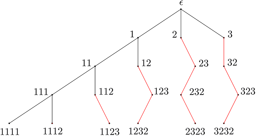
 is defined in (2-3). For example, if
$n = 4$
 (see Figure 1),

where
$ \Sigma _M^{4;1,1} = \{2323\} $
 and
$ \Sigma _M^{4;1,2} = \{3232\}$
 . Also,

and
$ \Sigma _M^{4;k,2} = \emptyset $
 for all
$2\leq k\leq 4$
 .
The graph of
$\Sigma _M^*$
 with
$ M $
 is defined in (4-1).

Figure 1 Long description
The diagram is a tree graph starting at a top root node labeled with the Greek letter epsilon.
Level 1: Three branches descend from epsilon to nodes labeled 1, 2, and 3 from left to right.
Level 2:
- Node 1 branches left to 11 and down to 12.
- Node 2 branches down to 23.
- Node 3 branches down to 32.
Level 3:
- Node 11 branches left to 111 and down to 112.
- Node 12 branches down to 123.
- Node 23 branches down to 232.
- Node 32 branches down to 323.
Level 4 (Leaf Nodes):
- Node 111 branches left to 1111 and down to 1112.
- Node 112 branches down to 1123.
- Node 123 branches down to 1232.
- Node 232 branches down to 2323.
- Node 323 branches down to 3232.
Visual styling: The leftmost path (epsilon to 1 to 11 to 111 to 1111) and the vertical branches from 1 to 12, 11 to 112, and 111 to 1112 are drawn with black lines. All other branching paths starting from nodes 12, 2, and 3 are drawn with red lines, often following a zigzag downward pattern.
Now, we calculate the entropy of the Markov tree-shift
$T = T_{\Sigma _M^*}$
 associated with a family
$\mathcal {R}$
 of relations, determined by
$(A_1, A_2, A_3)$
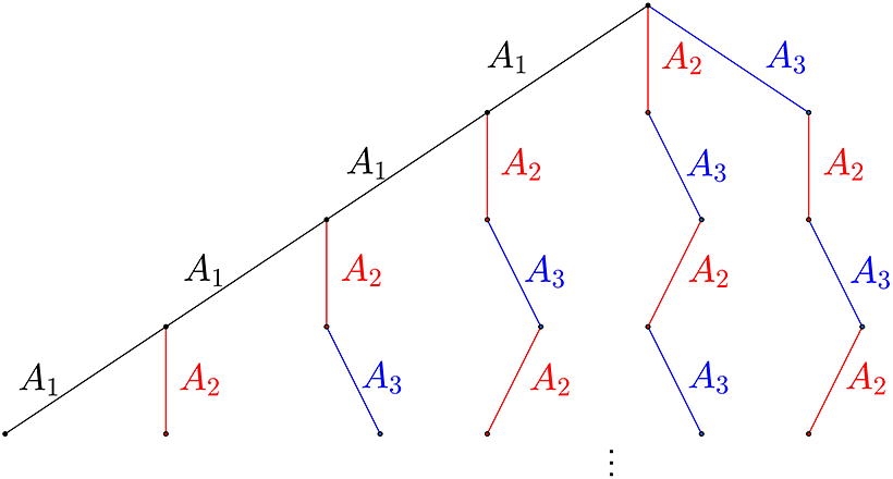
 (see Figure 2), with A being a finite set of labels. We simplify the notation
$u_{1;r,n}$
 to
$u_{r,n}$
 , where
$u_{1;r,n}$
 is defined in (3-12) for
$r=1,2$
 and
$n\in \mathbb {N}$
 . By Lemma 3.2,

Thus, for any
$\epsilon>0$
 , there exists
$N\in \mathbb {N}$
 such that for all
$n\geq N,$


and

The graph of the Markov tree-shift
$T=T_{\Sigma _M^*}$
 associated with a family
$\mathcal {R}$
 of relations, determined by
$(A_1,A_2,A_3)$
 and the matrix
$ M $
 is defined in (4-1).

First, we claim that

Note that for
$n\geq 1$
 ,

For example, when
$n=4$
 , we can express
$\Sigma _M^{\leq 4}$
 in the following form:

where

and

(see Figure 1 for
$D_4$
 (colored in red) and
$V_4$
 (colored in black)).
Then,

(see Figure 2).
By (4-2) and (4-5), we get that for any
$n\geq N,$


where
$c=\prod _{i=1}^{N-2}|A_{u_{2,i}}|$
 .
Dividing Inequality (4-6) by
$|\Sigma _M^{\leq n}|$
 and taking n to infinity,

Since
$\epsilon>0$
 is arbitrary, the inequality (4-4) holds.
Second, suppose T is TT. Then, there exists
$N'\in \mathbb {N}$
 such that
$A_u$
 is positive for all
$u\in \Sigma _M^*$
 with
$|u|\geq N'$
 . We claim that

Indeed,

For example, when
$n=4$
 and
$N'=2$
 (see Figure 1), we express
$\Sigma _M^{\leq 4}$
 in the following form:

where
$V_4'=\Sigma _M^{\leq 4}\setminus D_4'$
 and

Then,

Taking the logarithm of (4-8) and applying Inequality (4-3), we get for any
$n\geq N+N'$
 ,

where
$c'=\prod _{i=1}^{N'-2}\lvert A_{u_{2;N+1:N+i}}\rvert .$

Dividing Inequality (4-9) by
$|\Sigma _M^{\leq n}|$
 and taking n to infinity,

Since
$\epsilon>0$
 is arbitrary, the inequality (4-7) holds.
Finally, combining Inequalities (4-4) and (4-7),

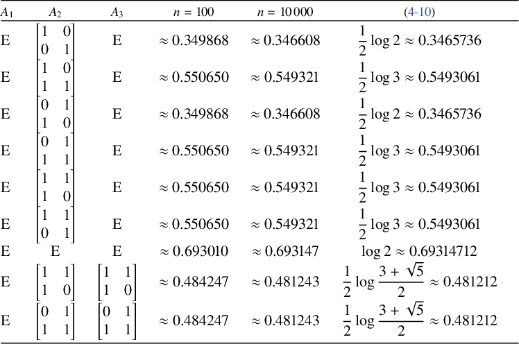
Now, we provide the results of the numerical computations. Figure 3 and Table 1 present the entropy of the Markov tree-shift
$ T = T_{\Sigma _M^*} $
 , which is TT. Let E be a
$2\times 2$
 full one matrix.
The graph shows the values of
$|\Sigma _M^{\leq n}|^{-1}\log | T_{\Sigma _M^{\leq n}}|$
 for
$1\leq n\leq 100$
 . The quantity
$|T_{\Sigma _M^{\leq n}}|$
 is a function of a family
$\mathcal {R}$
 of relations
$(\text {that is }|T_{\Sigma _M^{\leq n}}|=|T_{\Sigma _M^{\leq n}}(\mathcal {R})|)$
 , where the family
$\mathcal {R}_1$
 (respectively
$\mathcal {R}_2$
 ,
$\mathcal {R}_3$
 ,
$\mathcal {R}_4$
 ) is determined by
$(E,[1~0;0~1],E)\, (\text {respectively } (E,[1~0;1~1],E),(E,E,E),(E,[1~1;1~0],[1~1;1~0]) )$
 .

Figure 3 Long description
The horizontal x-axis is labeled n and ranges from 0 to 100. The vertical y-axis is labeled log absolute T sub Sigma M super less than or equal to n all over absolute Sigma M super less than or equal to n and ranges from 0.0 to 0.6. Four data series, represented by colored lines with circular markers, rise sharply from the origin and level off into horizontal plateaus.
* The green series, R sub 3, is the highest, converging to a red dashed line at log 2, approximately 0.69.
* The orange series, R sub 2, converges to a yellow dashed line at 1 half log 3, approximately 0.55.
* The purple series, R sub 4, converges to a dark blue dashed line at 1 half log open parenthesis 3 plus square root 5 close parenthesis all over 2, approximately 0.48.
* The blue series, R sub 1, is the lowest, converging to a green dashed line at 1 half log 2, approximately 0.35.
A legend on the right side maps the colors to the relations R sub 1 through R sub 4 and their corresponding mathematical limit constants.
Entropy of
$T_{\Sigma_M^*}$
 : numerical approximations and exact values.

Table 1 Long description
The table consists of six columns and nine data rows.
Column headers from left to right are: A sub 1, A sub 2, A sub 3, n = 100, n = 10,000, and a reference column for exact values (4-10).
Row 1: A sub 1 is E. A sub 2 is a 2 by 2 identity matrix (1, 0; 0, 1). A sub 3 is E. n = 100 is approximately 0.349868. n = 10,000 is approximately 0.346608. Exact value is 1/2 log 2, approximately 0.3465736.
Row 2: A sub 1 is E. A sub 2 is matrix (1, 0; 1, 1). A sub 3 is E. n = 100 is approximately 0.550650. n = 10,000 is approximately 0.549321. Exact value is 1/2 log 3, approximately 0.5493061.
Row 3: A sub 1 is E. A sub 2 is matrix (0, 1; 1, 0). A sub 3 is E. n = 100 is approximately 0.349868. n = 10,000 is approximately 0.346608. Exact value is 1/2 log 2, approximately 0.3465736.
Row 4: A sub 1 is E. A sub 2 is matrix (0, 1; 1, 1). A sub 3 is E. n = 100 is approximately 0.550650. n = 10,000 is approximately 0.549321. Exact value is 1/2 log 3, approximately 0.5493061.
Row 5: A sub 1 is E. A sub 2 is matrix (1, 1; 1, 0). A sub 3 is E. n = 100 is approximately 0.550650. n = 10,000 is approximately 0.549321. Exact value is 1/2 log 3, approximately 0.5493061.
Row 6: A sub 1 is E. A sub 2 is matrix (1, 1; 0, 1). A sub 3 is E. n = 100 is approximately 0.550650. n = 10,000 is approximately 0.549321. Exact value is 1/2 log 3, approximately 0.5493061.
Row 7: A sub 1 is E. A sub 2 is E. A sub 3 is E. n = 100 is approximately 0.693010. n = 10,000 is approximately 0.693147. Exact value is log 2, approximately 0.69314712.
Row 8: A sub 1 is E. A sub 2 is matrix (1, 1; 1, 0). A sub 3 is matrix (1, 1; 1, 0). n = 100 is approximately 0.484247. n = 10,000 is approximately 0.481243. Exact value is 1/2 log of the fraction (3 plus square root of 5) all over 2, approximately 0.481212.
Row 9: A sub 1 is E. A sub 2 is matrix (0, 1; 1, 1). A sub 3 is matrix (0, 1; 1, 1). n = 100 is approximately 0.484247. n = 10,000 is approximately 0.481243. Exact value is 1/2 log of the fraction (3 plus square root of 5) all over 2, approximately 0.481212.
The following example shows that the equality ‘
$=$
 ’ in Theorem 1.3 is not sufficient without TT.
Example 4.2. Let
$\Sigma _M^*$
 be a monoid with

Suppose
$A=\{a,b,c,d\}$
 and
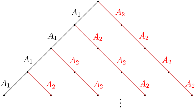
$T=T_{\Sigma _M^*}$
 (see Figure 4) is a Markov tree-shift associated with a family
$\mathcal {R}$
 of relations, determined by
$(A_1,A_2)$
 , where

The graph of a Markov tree-shift
$T=T_{\Sigma _M^*}$
 associated with a family
$\mathcal {R}$
 of relations, determined by
$(A_1,A_2)$
 , and the matrix M is defined in (4-11).

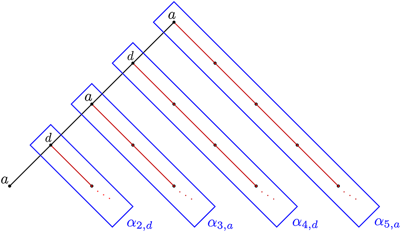
To clearly calculate the entropy, we introduce some notation. Let
$\alpha _{n,a}=|\{w_1w_2\cdots w_n\in \Sigma _{A_2}^n:w_1=a\}|$
 and
$\beta _{n,a} =|\{ t \in T_{\Sigma _M^{\leq n}} : t(\epsilon ) = a \}|$
 for
$a\in A$
 .
In this case, we have
$|\Sigma _M^{\leq n}|=({(n+1)(n+2)}/{2})$
 ,
$\alpha _{n,a}=2^{n-1}=\alpha _{n,b}$
 ,
$\alpha _{n,c}=\iota _1\mu _1^{n}+\iota _2\mu _2^{n}$
 , and
$\alpha _{n,d}=\iota _1\mu _1^{n-1}+\iota _2\mu _2^{n-1}$
 , where
$\iota _1=({5+\sqrt {5}})/{10}$
 ,
$\iota _2=({5-\sqrt {5}})/{10}$
 ,
$\mu _1=({1+\sqrt {5}})/{2}$
 , and
$\mu _2=({1-\sqrt {5}})/{2}$
 . From observing Figure 5, we obtain the following:

where
$d_{n,j}=\prod _{k=1}^{n+1}(\iota _1+\iota _2({\mu _2}/{\mu _1})^{2k+i-j})$
 for
$j=1,2,3$
 . It is straightforward to observe that for each
$i=0,1,2,3$
 ,

Thus,

This example suggests that if T is not TT, then the ‘
$=$
 ’ may be replaced by ‘
$<$
 ’.
The graph of a Markov tree-shift T has its root labeled a.

Acknowledgments
We would like to sincerely thank the anonymous referee for providing helpful suggestions for the first draft of this article. These improve the readability of the paper. All authors thank the National Center for Theoretical Sciences for partial support.