Introduction
Body size is a key trait of all organisms and correlates with almost every aspect of their physiology, ecology, and evolution (Roy Reference Roy2008). An organism's size reflects how it acquires and processes energy and provides valuable information regarding the resource partitioning between species along a range size (Peters Reference Peters1983; Ernest Reference Ernest2005; Anderson-Teixeira et al. Reference Anderson-Teixeira, Savage, Allen and Gillooly2009). The body-size distribution (BSD) of species in a guild, clade, or assemblage reflects their niche requirements and is the macroecological and macroevolutionary outcome of the many drivers that constrain body size (Calder Reference Calder1984; Roy et al. Reference Roy, Jablonski and Martien2000). The “null” shape of the BSD fits to a lognormal distribution (McKinney Reference McKinney and McNamara1990; McShea Reference McShea1994; Marquet and Taper Reference Marquet and Taper1998; Maurer Reference Maurer1998, Reference Maurer, Blackburn and Gaston2003; Kozłowski and Gawelczyk Reference Kozłowski and Gawelczyk2002; Maurer and Marquet Reference Maurer, Marquet, Felisa and Lyons2013), in which the minimum and maximum sizes are constrained by energetic requirements, biotic interactions, and environmental drivers (Brown et al. Reference Brown, Calder and Kodric-Brown1978, Reference Brown, Marquet and Taper1993; Schmidt-Nielsen Reference Schmidt-Nielsen1984; Marquet and Taper Reference Marquet and Taper1998; Allen et al. Reference Allen, Garmestani, Havlicek, Marquet, Peterson, Restrepo, Stow and Weeks2006; Maurer and Marquet Reference Maurer, Marquet, Felisa and Lyons2013; Smith et al. Reference Smith, Payne, Heim, Balk, Finnegan, Kowalewski, Lyons, McClain, McShea, Novack-Gottshall, Anich and Wang2016) and the height (or modal size) is the most common bin size used by different species or individuals (Maurer and Marquet Reference Maurer, Marquet, Felisa and Lyons2013). BSDs have been described for several marine assemblages (Warwick Reference Warwick1984; Kendall et al. Reference Kendall, Warwick and Somerfield1997; Roy et al. Reference Roy, Jablonski and Martien2000; Hildrew et al. Reference Hildrew, Raffaelli and Edmonds-Brown2007; Baltanas and Danielopol Reference Baltanas and Danielopol2013; Gearty et al. Reference Gearty, McClain and Payne2018) and tend to change in response to nutrient availability, the type of ecosystem, and the level of disturbance (Warwick Reference Warwick1984; McClain et al. Reference McClain, Gullett, Jackson-Ricketts and Unmack2012). For instance, lower levels of available energy result in assemblages of smaller-sized organisms (e.g., right-skewed BSD), with strategies that enable them to survive with lower levels of foraging and/or with mechanisms to cope with starvation (McClain Reference McClain2004; McClain et al. Reference McClain, Gullett, Jackson-Ricketts and Unmack2012). Assemblages that occur under higher levels of productivity have diverse taxa of larger-sized individuals and expensive life strategies (e.g., left-skewed BSD) (Rex and Etter Reference Rex and Etter1998; Roy et al. Reference Roy, Jablonski and Martien2000; McClain Reference McClain2004; McClain et al. Reference McClain, Gullett, Jackson-Ricketts and Unmack2012, Reference McClain, Barry and Webb2018). Therefore, the BSD may provide valuable insights into the determinants of species structure through episodes of environmental change, such as past biotic crises.
Body size is highly susceptible to environmental change (Gardner et al. Reference Gardner, Peters, Kearney, Joseph and Heinsohn2011). In marine animals, global warming is expected to lead to a reduction in body size due to the impacts of temperature rise, lower concentrations of dissolved oxygen, lower pH, and changes in productivity (Sheridan and Bickford Reference Sheridan and Bickford2011). Body-size reduction has also been demonstrated in a range of marine taxa during several past mass extinction events (Urbanek Reference Urbanek1993; Twitchett and Barras Reference Twitchett and Barras2004; He et al. Reference He, Twitchett, Zhang, Shi, Feng, Yu, Wu and Peng2010; Martinez-Diaz et al. Reference Martinez-Diaz, Phillips, Nyborg, Espinosa, Tavora, Centeno-Garcia and Vega2016). The temporary reduction in the body size of surviving species in the immediate aftermath of an extinction event was termed the “Lilliput Effect” by Urbanek (Reference Urbanek1993), and although there are several potential reasons why such a phenomenon could be recorded in the fossil record (Twitchett Reference Twitchett2007; Harries and Knorr Reference Harries and Knorr2009), in most cases, the smallest sizes are associated with peak temperatures and global warming, and so likely reflect responses to environmental change. During the recovery from mass extinction events, the sizes of surviving taxa and newly originating taxa increase as environmental conditions ameliorate (Payne Reference Payne2005; Barras and Twitchett Reference Barras and Twitchett2007; Novack-Gottshall Reference Novack-Gottshall2008; Metcalfe et al. Reference Metcalfe, Twitchett and Price–Lloyd2011; He et al. Reference He, Shi, Yang, Zhang, Yue, Xiao, Wu, Chen and Wu2016; Sigurdsen and Hammer Reference Sigurdsen and Hammer2016; Brom et al. Reference Brom, Salamon and Gorzelak2018; Atkinson et al. Reference Atkinson, Wignall, Morton and Aze2019; Atkinson and Wignall Reference Atkinson and Wignall2020; Foster et al. Reference Foster, Gliwa, Lembke, Pugh, Hofmann, Tietje, Varela, Foster, Korn and Aberhan2020).
Theoretical models would suggest that BSD would emerge throughout a cladogenetic diffusion model of species body size (McKinney Reference McKinney and McNamara1990, Reference McKinney1997; McShea Reference McShea1994; Clauset and Erwin Reference Clauset and Erwin2008), in which small-bodied species are expected to be common relative to larger-bodied species (Stanley Reference Stanley1973, Reference Stanley1979; Hayami Reference Hayami1978; Gould Reference Gould1988; McShea Reference McShea1994; Monroe and Bokma Reference Monroe and Bokma2013) (Fig. 1). However, the size diffusion process can be punctuated by episodes of biotic crisis (Gould Reference Gould1988; McKinney Reference McKinney and McNamara1990), and two possible BSD shapes may result depending on the selective nature of the disturbance (Fig. 1). If the extinction is size selective, then a curtailed BSD would result due to extinction of larger taxa, whereas extinction that is random with respect to size could lead to a platykurtic size distribution (McKinney Reference McKinney and McNamara1990) (Fig. 1). Although a number of previous studies have addressed size change during extinction events, most of the work has focused on changes within individual taxa. Hitherto, little attention has been paid to the relationship between the dynamics of within-lineage size change and the effect on the evolution of the overall BSD of species arranged along the entire size spectrum, or how the overall BSD is modified by a mass extinction event.
Body-size distribution (BSD) model across evolutionary time. Based on the model of McKinney (Reference McKinney and McNamara1990), the scheme shows how cladogenetic diffusion processes give rise to BSDs. Small sizes are more common and tend to accumulate around the modal size, while clades of larger sizes arriving gradually into the community expand the tail of the distribution. An extinction event punctuates the diffusion process, generating two outcomes depending on whether the extinction is selective or not. Larger sizes are eliminated under selective extinctions, while a nonselective event generates a flatter BSD due to a random probability of extinction.

Here, we study how the BSD of bivalves was affected by the Late Triassic mass extinction event (LTE) (~201.5 Ma; Wotzlaw et al. Reference Wotzlaw, Guex, Bartolini, Gallet, Krystyn, McRoberts, Taylor, Schoene and Schaltegger2014), the second biggest biodiversity loss of the Phanerozoic (Kocsis et al. Reference Kocsis, Reddin, Alroy and Kiessling2019). The LTE is directly linked to an intense greenhouse event (McElwain et al. Reference McElwain, Beerling and Woodward1999; Berner and Beerling Reference Berner and Beerling2007; Kidder and Worsley Reference Kidder and Worsley2010; Davies et al. Reference Davies, Marzoli, Bertrand, Youbi, Ernesto and Schaltegger2017; Dunhill et al. Reference Dunhill, Foster, Azaele, Sciberras and Twitchett2018) triggered by massive injection of CO2 into the ocean–atmosphere system (van de Schootbrugge et al. Reference van de Schootbrugge, Payne, Tomasovych, Pross, Fiebig, Benbrahim, Follmi and Quan2008; Ruhl and Kurschner Reference Ruhl and Kurschner2011; Ruhl et al. Reference Ruhl, Bonis, Reichart, Damste and Kurschner2011; Blackburn et al. Reference Blackburn, Olsen, Bowring, McLean, Kent, Puffer, McHone, Rasbury and Et-Touhami2013) during eruption of the Central Atlantic Magmatic Province (CAMP) (Fig. 1) (Zaffani et al. Reference Zaffani, Jadoul and Rigo2018). Secondary environmental effects resulting from global warming have also been inferred, including ocean acidification (Crne et al. Reference Crne, Weissert, Gorican and Bernasconi2011), widespread anoxia (Jaraula et al. Reference Jaraula, Grice, Twitchett, Böttcher, LeMetayer, Dastidar and Opazo2013; He et al. Reference He, Dal Corso, Newton, Wignall, Mills, Todaro, Di Stefano, Turner, Jamieson, Randazzo, Rigo, Jones and Dunhill2020), and rapid sea-level change (Hallam and Wignall Reference Hallam and Wignall1999). Evidence of body-size changes has been recorded in a variety of taxa at different spatial and temporal scales during the LTE (Dommergues et al. Reference Dommergues, Montuire and Neige2002; Barras and Twitchett Reference Barras and Twitchett2007; Atkinson et al. Reference Atkinson, Wignall, Morton and Aze2019; Atkinson and Wignall Reference Atkinson and Wignall2020), but no studies have examined how the ecological collapse associated with the LTE modified the BSD of marine organisms at local and regional scales.
Using data collected from three well-correlated study sites within the United Kingdom, we assess (1) whether the body sizes of individual bivalve taxa and the BSD as a whole changed significantly through the LTE, (2) whether the patterns and timing of changes varies between sites, and (3) whether the LTE was a size-selective extinction, by testing the null hypothesis that the BSD of bivalves does not exhibit measurable changes through the LTE.
Materials and Methods
Sample Sites and Stratigraphy
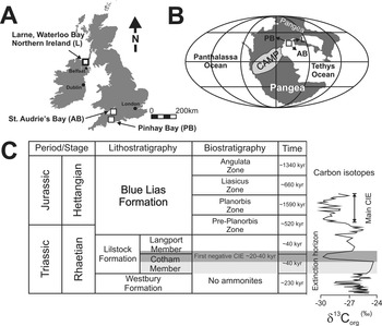
Fossil bivalves measured in this study came from three Triassic–Jurassic marine successions in the United Kingdom (Supplementary Fig. S1). The first study site was St. Audrie's Bay, Somerset, southwest England (51°10′0.36″N, 3°7′8.2″W) (Fig. 2), which has one of the most complete, well-known, and well-preserved Triassic–Jurassic marine fossil records (Warrington et al. Reference Warrington, Cope and Ivimey-Cook2008). The second site sampled was Larne, County Antrim, Northern Ireland (54°51′26″N, 5°48′18″W), which has a ~115-m-thick stratigraphically expanded section that spans from the upper part of the Mercia Mudstone Group (Triassic, Norian) through to the Bucklandi Zone of the Lias Group (Jurassic, Sinemurian) and is cut by minor faults (Simms and Jeram Reference Simms and Jeram2007). Only 62 m were sampled, from the base of Westbury Formation to the Liasicus Zone of the Blue Lias Formation (Supplementary Fig. 1). The third section extends from Pinhay Bay, Devon, to Lyme Regis, Dorset, southern England (50°42′44.94″N, 2°58′2.81″W) and spans from the Rhaetian upper Lilstock Formation through the Hettangian–Sinemurian Blue Lias Formation (e.g., Hallam Reference Hallam1960; Fig. 2). Only 21 m were sampled from the Pinhay Bay–Lyme Regis section: from the base of the Langport Member (Lilstock Formation) to the Angulata Zone (Blue Lias Formation). The studied sections contain abundant ammonites that enable correlation with each other and with other Triassic–Jurassic sections worldwide. Details relating to the geologic and paleoenvironmental setting, extinction horizon, and Triassic/Jurassic boundary are summarized in the Supplementary Text.
Stratigraphy, location, and paleogeography of study sites sampled in the United Kingdom. A, Sampled localities in this study (white squares). B, Global view of Pangea showing the paleogeographic location of United Kingdom during the Rhaetian–Hettangian (white square). C, Generalized stratigraphic and biostratigraphic scheme of the Triassic–Jurassic of the United Kingdom, with a carbon isotope curve from the section at St. Audrie's Bay, UK. The shaded gray area indicates the extinction horizon, which coincides with the first negative carbon isotope excursion (CIE) (Hesselbo et al. Reference Hesselbo, Robinson and Surlyk2004). Line with arrowheads indicates the position of the main negative carbon isotope excursion (Main CIE) (Hesselbo et al. Reference Hesselbo, Robinson and Surlyk2004); the durations of each unit were obtained from Ruhl et al. (Reference Ruhl, Deenen, Abels, Bonis, Krijgsman and Kurschner2010), Bonis et al. (Reference Bonis, Ruhl and Kurschner2010), Wotzlaw et al. (Reference Wotzlaw, Guex, Bartolini, Gallet, Krystyn, McRoberts, Taylor, Schoene and Schaltegger2014), and Weedon et al. (Reference Weedon, Page and Jenkyns2019). CAMP, Central Atlantic Magmatic Province.

Sampling Methods and Body-Size Measurements
Morphometric measurements of bivalves were collected from the base of the Westbury Formation (Rhaetian) to the Angulata Zone (Hettangian) in St. Audrie's Bay; from the base of the Langport Member to the Angulata Zone in Pinhay Bay; and from the Westbury Formation to the Liasicus Zone (Hettangian) in Larne (Supplementary Fig. 1, Supplementary Files). One sample of 1.5 ± 0.2 kg was collected from each major lithology (limestone and mudstone) on average every 1.98 ± 0.5 m. In addition, to increase the sample size of each stratigraphic horizon, individual measurements were made in the field from bedding plane exposures using a tape measure (SE ± 0.5 mm).
Samples from the different lithologies were processed in different ways. Limestone rock samples of 1.5 ± 0.2 kg (with dimensions of ca. 20 cm length × 20 cm width ×15 cm height) were cut perpendicular to the bedding plane surface, generating slabs approximately 8 cm wide (see Supplementary Fig. 2A). Using a chisel-tipped hammer, each slab (20 × 15 × 8 cm) was then split parallel to the bedding plane, which generated sampling plates of approximately 2 × 20 × 8 cm with specimens exposed on the surfaces of each slab for potential measurement (see Supplementary Fig. 2A). This technique minimized damage to the specimens in order to preserve entire individuals for measurement.
In contrast, sandstone and mudstone samples were broken into ~50 cm2 chips, and water was used to soak the rock and separate the fossils without damaging them. All the bivalves were classified from published information (Swift and Martill Reference Swift and Martill1999; Hodges Reference Hodges2000; Lord and Davis Reference Lord and Davis2010). In all cases, measurements of the length (maximum distance on the anterior-posterior axis) and height (maximum distance on the dorsal-ventral axis) were recorded only from complete, well-preserved specimens (Supplementary Fig. 2B,C). All morphometric variables were measured using electronic calipers (SE ± 0.01 mm).
Data Analysis
The body size of each specimen was calculated as the geometric mean (i.e., the square root of the product of length and width) and log2 transformed to reduce the heteroscedasticity and to facilitate graphic representation (Piazza et al. Reference Piazza, Duarte, Renaudie and Aberhan2019). Changes in the body sizes of bivalves through the LTE were evaluated in four different ways.
Body-Size Distribution across Space and Time
To evaluate body-size changes through the LTE and to test whether any changes occurred synchronously at the different localities, mean body sizes per species were pooled within each stratigraphic unit. The shapes of the BSDs of each stratigraphic unit were examined graphically by plotting standard statistical metrics such as the coefficient of variation, skewness, maximum and minimum values, and median. A Shapiro-Wilk test was performed to test the normality of each distribution. A Kruskal-Wallis test was performed to detect significant differences in median values between each stratigraphic unit. A test of homogeneity of variance (Bartlett's test) was performed on each stratigraphic unit to evaluate whether the changes in the variance between localities were synchronous. Finally, the residuals of the body sizes of each stratigraphic unit were calculated and plotted to graphically assess changes in BSD. Each residual value was calculated as the difference between the grand mean ( $\bar{X}$ = 12.63 mm; i.e., the average size of entire dataset) minus the average body size of each species present in each stratigraphic unit. To test significant differences in the residual distribution of each stratigraphic unit, 95% confidence intervals of the residuals were estimated by an iterative random resampling (9999 iterations). Differences were considered significant when the residual values fell outside the confidence intervals.
Taxonomic and Size Selectivity
To test whether the LTE was size selective, each bivalve taxon was assigned to one of three extirpation categories: (1) survivors, that is, those recorded in at least one locality and stratigraphic unit from both the pre-extinction and the recovery intervals; (2) colonizers, that is, those taxa that only occur after the extinction event (i.e., between the Cotham Member of the Lilstock Formation and Angulata Zone of the Blue Lias Formation). The extinction horizon coincides with the onset of a negative δ13Corg excursion that spans from the upper Cotham Member to the lower Langport Member (20–40 kyr) (Ruhl et al. Reference Ruhl, Deenen, Abels, Bonis, Krijgsman and Kurschner2010) and is characterized by high species turnover and low diversity (Mander et al. Reference Mander, Twitchett and Benton2008; Ruhl et al. Reference Ruhl, Deenen, Abels, Bonis, Krijgsman and Kurschner2010; Thibodeau et al. Reference Thibodeau, Ritterbush, Yager, West, Ibarra, Bottjer, Berelson, Bergquist and Corsetti2016; Atkinson and Wignall Reference Atkinson and Wignall2019) (see Fig. 2C and Supplementary Fig. S1). Finally, (3) extirpated taxa (hereafter referred to as “victims”) are those that recorded their last appearance either before, during, or after the LTE (i.e., from the upper Westbury Formation to the Langport Member of the Lilstock Formation). To detect significant changes in the BSD across the LTE, the coefficient of variation (i.e., standard deviation divided by the mean) was calculated for each category in each stratigraphic unit. In addition, residual values were calculated for each stratigraphic unit to track and assess the changes in BSD through time. For all dispersion parameters, the statistical differences between different stratigraphic units were evaluated through the estimation of 95% confidence intervals estimated by iterative random resampling (9999 iterations). Differences between successive bins were considered significant when their confidence intervals did not overlap.
Studies of the fossil record have demonstrated that selective extinction against specific lineages or ecological traits would drive important ecological and evolutionary modifications (Hallam and Wignall Reference Hallam and Wignall1997; Jablonski Reference Jablonski2008; Janevski and Baumiller Reference Janevski and Baumiller2009; Harnik Reference Harnik2011; Orzechowski et al. Reference Orzechowski, Lockwood, Byrnes, Anderson, Finnegan, Finkel, Harnik, Lindberg, Liow, Lotze, McClain, McGuire, O'Dea, Pandolfi, Simpson and Tittensor2015; Payne et al. Reference Payne, Bush, Chang, Heim, Knope and Pruss2016a,Reference Payne, Bush, Heim, Knope and McCauleyb). Substantial differences with respect to trait between taxonomic groups could change the distribution of the species within genera, families, and orders (Jablonski and Raup Reference Jablonski and Raup1995; Aberhan and Baumiller Reference Aberhan and Baumiller2003; Smith and Roy Reference Smith and Roy2006; Rivadeneira and Marquet Reference Rivadeneira and Marquet2007; Finnegan et al. Reference Finnegan, Heim, Peters and Fischer2012; Ros and Echevarria Reference Ros and Echevarria2012; Harnik et al. Reference Harnik, Fitzgerald, Payne and Carlson2014; Dishon et al. Reference Dishon, Grossowicz, Krom, Guy, Gruber and Tchernov2020). To test existence of phylogenetic effect in size selectivity in bivalves across the LTE, two methodological steps based on Rivadeneira and Marquet (Reference Rivadeneira and Marquet2007) were implemented. First, a Moran's autocorrelogram analysis was used to evaluate whether the differences in body size among species are related to their taxonomic distance (Gittleman and Kot Reference Gittleman and Kot1990; Rivadeneira and Marquet Reference Rivadeneira and Marquet2007). It has been suggested that this method is a good analytical strategy to assess whether a phylogenetic control may exist on quantitative traits when phylogenetic information is not available (Gittleman and Kot Reference Gittleman and Kot1990). In this case, a typical phylogenetic signature is evident by the decay in the rescaled Moran's I toward higher taxonomic levels (Gittleman and Kot Reference Gittleman and Kot1990; Rivadeneira and Marquet Reference Rivadeneira and Marquet2007). High phylogenetic inertia is interpreted as a high level of similarity among taxa or low variation of the trait between lineages (Gittleman and Kot Reference Gittleman and Kot1990). If phylogenetic inertia is identified at a taxonomic level, the second step is to identify the selectivity. For that, the body size of each species in each extirpation category is regressed against the mean body size of the taxonomic level with the most variation. If the number of extirpated taxa, for instance, increases significantly along with larger order, then we would be recording a selective extirpation. Linear square regressions were fit to each trait value, and a linear regression with a 0 intercept was fit to all data points. Finally, all the slopes and intercepts were compared. Moran's autocorrelogram analysis was estimated using the package APE (Paradis and Schliep Reference Paradis and Schliep2019), implemented in R v. 3.6.0 (R Core Team 2019).
Density Distribution and Generalized Linear Model of Different Tiers
All the recorded bivalves were classified according to their tiering habit (i.e., semi-infaunal, infaunal, and epifaunal) from information available in the Paleobiology Database (PBDB; https://paleobiodb.org) and Mander and Twitchett (Reference Mander and Twitchett2008). The body sizes of all individuals of each species were pooled to capture the complete size distribution of each tier in each stratigraphic unit. The modality of the BSDs in each stratigraphic unit was examined by plotting the frequency distribution of each mode of life with a bin size of 0.25 on a log2 scale. Subsequently, a continuous distribution to each mode of life was fit by using a combination of kernel density estimation and smoothed bootstrap resampling (based on 1000 randomizations) (Manly Reference Manly1996). This procedure approximates the probability density function of a random variable by determining the optimum modality of the data, testing whether a distribution with k + 1 modes fits significantly better than a distribution with k modes (Silverman Reference Silverman1981; Manly Reference Manly1996). In addition, measures of skewness and kurtosis were estimated for each distribution. A Lilliefors (Kolmogorov-Smirnov) test was performed to test the normality of each distribution, and a Kolmogorov-Smirnov two-sample test (K-S test) was used to compare BSDs between pairs of consecutive stratigraphic units. In this case, the probability values (p) were adjusted by the Bonferroni correction.
Generalized linear models (GLMs), assuming a Gaussian distribution with a log-link function, were used to examine differences in mean body size between the different tiers in each stratigraphic level. A full factorial design with two factors was implemented: factor 1 (tiering) had three levels (i.e., infaunal, semi-infaunal, and epifaunal); factor 2 (stratigraphic unit) had seven levels (horizons); while body size was used as the response variable. A Gaussian distribution was fit by Akaike information criterion (AIC = −1420.28), using the package propagate (Spiess Reference Spiess2018) implemented in R v. 3.6.0 (R Core Team 2019). Finally, a Newman-Keuls test was performed as an a posteriori test to determine which groups generated the differences.
Null Model
An unweighted null model was constructed to assess whether any changes in recorded body size could be explained purely by random assembly. A null model is based on randomization of ecological data to evaluate patterns of some ecological or evolutionary process of interest. Here, the randomization was designed to produce a pattern that would be expected in the absence of a particular ecological mechanism, with the aim of emphasizing the potential importance of stochastic mechanisms in producing natural patterns (Gotelli and Graves Reference Gotelli and Graves1996). The null model was built by unweighted randomization of the rows and columns (n × m) of a matrix of individual sizes arranged by species (n) and samples (m). For each randomization, an average value was produced for each sample (or sampling horizon), and after 9999 iterations, a grand mean and 2.5% and 97.5% percentiles were computed for each sample. Differences in mean body size were considered significant when confidence intervals did not overlap. This procedure was performed for each locality. All the analyses were performed using R v. 3.6.0 (R Core Team 2019). R code for the null model is described in the Supplementary Text.
Results
Taxonomic Richness
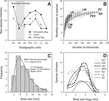
A total of 2247 individuals belonging to 39 species and 29 genera of bivalves were sampled in this study (see Supplementary Dataset), with an average of 15 (±2) species per stratigraphic unit. Lowest richness was recorded in the Cotham Member and in the Angulata Zone, with 9 and 10 species respectively (Fig. 3A,B). The first drop in richness coincides with the extinction horizon (Cotham Member; Fig. 2B). In contrast, highest richness was recorded immediately after the extinction event (Langport Member); here, the taxonomic richness of bivalves increased by 90% (19 species) in less than ~100 kyr (Bonis et al. Reference Bonis, Ruhl and Kurschner2010). Species richness in the Westbury Formation and the pre-Planorbis, Planorbis, and Liasicus Zones fluctuated between 17 and 18 species, with no significant differences (Fig. 3A,B).
Species richness and body-size patterns of bivalves through the Triassic–Jurassic of the UK sections. A, Raw species richness recorded for each stratigraphic unit and locality. B, Rarefied richness. Average values (±95% confidence intervals) of species richness estimated as sampling size increases. Significant differences were assumed if 95% confidence intervals did not overlap. WF, Westbury Formation; CM, Cotham Member; LM, Langport Member; PPZ, pre-Planorbis Zone, PZ, Planorbis Zone, LZ, Liasicus Zone, AZ, Angulata Zone. C, Body-size distribution of all bivalves recorded across the Triassic–Jurassic sections. A lognormal distribution was fit to the observed BSD. D, Bivariate relationships between body size and raw species richness plotted for each stratigraphic unit. Each line represents the kernel density fit to the data.

Body-Size Distribution across Time and Space
The BSD of all bivalve species (n = 39) fits to a lognormal distribution (r 2 = 0.87, p < 0.05) (Fig. 3C), with a modal size ~8 mm, significantly right-skewed with size distributions that range from minimum and maximum sizes of 3.40 and 30.8 mm, respectively. The relationship between species richness and body size (Fig. 3D) exhibits a platykurtic distribution during the extinction event (Cotham Member). Assemblages from the immediate aftermath of the LTE (Langport Member) record a leptokurtic distribution with a modal size of ~3.75 log2 mm (Fig. 3D). Most assemblages from the pre-extinction and recovery intervals record mesokurtic BSDs (mode ~3.1 log2 mm), except for the pre-Planorbis Zone, which exhibits a bimodal distribution (Fig. 3D). The Angulata Zone recorded a low species number but reports a higher mode (~4 log2 mm) and mesokurtic shape (Fig. 3D).
Bivalve assemblages from the Cotham Member record the lowest median size of all stratigraphic units in this study (Fig. 4A). Despite this, the Kruskal-Wallis test did not detect significant differences in median body size across the extinction event (χ2 = 5.51, p > 0.48; Fig. 4A). However, the dispersal parameters and shape of the BSD change significantly through the Triassic–Jurassic interval (Fig. 4B–D).
Temporal changes in the dispersal parameters of the body-size distributions (BSDs) of 37 Triassic–Jurassic bivalve taxa recorded in this study. A, Residual values of the log2 body size grouped by stratigraphic unit; each point represents one species, with each symbol indicating the locality from which it was sampled (St. Audrie's Bay; Larne, Northern Ireland; and Pinhay Bay). Log2 mean body size ± SE is indicated for each stratigraphic unit. Zero on the y-axis represents the grand mean estimated from all species. Dashed lines are 95% confidence intervals estimated by bootstrapping with replacement (9999 iterations). B, Mean coefficient of variation of body size for each stratigraphic unit (-●-). Thin lines are 95% confidence intervals estimated by the bootstrapping procedure. C, Minimum (Min.), mean (Mean: -●-), and maximum (Max.) size for each stratigraphic unit. D, Skewness of the BSDs for each stratigraphic unit. Positive values indicate a right skew with a long tail of the data to the right; negative values indicate a left skew to the data. Size kernel–density plots (pale gray) show changes in the BSD between each stratigraphic unit. Key to stratigraphic units as in Fig. 3.

In the Westbury Formation, the BSD of bivalves is centered around the grand mean and lies within the confidence intervals, despite its slightly right-skewed distribution (Fig. 4D, Table 1). However, during the Cotham Member, the coefficient of variation significantly increases (Fig. 4B) due to the occurrence of some smaller species that skew the distribution toward negative values (Fig. 4C,D, Table 1). The Langport Member assemblage records the highest leptokurtic BSD, with little size variation and a significant negative skew (Fig. 4B,D, Table 1, Supplementary Table 1), due to all species being clustered around the grand mean size in the extinction aftermath. The pre-Planorbis Zone records an expansion of the size spectrum, shown by an increase in the coefficient of variation, due to the occurrence of relatively larger taxa, but it retains a negative skew due to the overall high dominance of small taxa in the assemblage (Fig. 4, Table 1). The Planorbis and Liasicus Zones record a further significant expansion in variance, due to the high occurrence of even larger taxa in the assemblages (Fig. 4B,C, and Table 1). The Angulata Zone records the largest average sizes with a significant right-skewed distribution and a significant reduction in the coefficient of variation (Fig. 4, Table 1). Analysis of the homogeneity of body-size variance showed no significant differences between localities, indicating that the BSDs of bivalves expanded or contracted synchronously at the different study sites (Supplementary Table 2).
Statistical descriptors of the body size distributions (BSDs) of the bivalve species recorded in each stratigraphic unit. All size values are expressed in log2. S-W, Shapiro-Wilk test values. No significant differences from a normal distribution were detected, critical α value = 0.05. WF, Westbury Formation; CM, Cotham Member (Lilstock Formation); LM, Langport Member (Lilstock Formation); and Blue Lias Formation ammonite zones: PPZ, pre-Planorbis Zone; PZ, Planorbis Zone; LZ, Liasicus Zone; AZ, Angulata Zone.

Selectivity
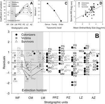
The coefficient of variation in the BSDs of victims and survivors is slightly higher in the Cotham Member than in the underlying Westbury Formation (~62%; Fig. 5A). Subsequently, during the Langport Member, variation of victims, survivors, and colonizers decreased (~40%). During the overlying Blue Lias Formation, the colonizers and survivors record gradual increases in their dispersion to a peak in the Liasicus Zone (~83%), followed by a decrease of 37% in the Angulata Zone (Fig 5A).
Body size and survivorship in bivalves during the Late Triassic mass extinction event and Hettangian recovery. A, The coefficient of variation for each extinction category through time. Thicker lines represent the mean value of the coefficient of variation, while the thinner lines represent the 95% confidence intervals estimated by bootstrapping. B, The residual values of log2 body size for each extinction category (survivors, victims, and postextinction colonizers). Each point represents the residual value of a single species within each stratigraphic unit. Zero on the y-axis represents the grand mean size estimated from all species. Dashed line is the 95% confidence intervals, estimated by bootstrapping. Black arrows indicate a reduction in size during the extinction horizon (shaded gray). Key to stratigraphic units as in Fig. 3. As, Astarte sp.; Ca, Camptonectes sp.; CR, Cardinia regularis; Cas, Cassianella sp.; CV, Chlamys valoniensis; Da, Dacryomya sp. GO, Gervillella ornata; GrO, Gryphaea obliquata.; GH, Grammatodon hettangiensis; IC, Isocyprina concentricum; IE, Isocyprina ewaldi; LB, Liostrea bristovi; LH, Liostrea hisingeri; MCa, Mactromya cardioides; Me, Mesomiltha sp.; MH, Modiolus hillanus; MM, Modiolus minimus; MS, Modiolus sodburiensis; Msp, Modiolus sp.; MV, Modiolus ventricosus; MY, Myoconcha psilonoti; MC, Mytilus cloacinus; OF, Oxytoma fallax; PE, Palaeoneilo elliptica; PN, Palaeonucula navis; Pe, Permophorus elongatus; Ph, Pholadomya sp.; PA, Placunopsis alpina; PG, Plagiostoma giganteum; PP, Plagiostoma punctatum; Pl, Pleuromya sp.; PR, Protocardia rhaetica; PD, Pseudolimea duplicata; Pt, ?Pteromya sp.; PCr, Pteromya crowcombeia; PL, Pteromya langportensis; RC, Rhaetavicula contorta; RB, Rollieria bronni; RT, Ryderia texturata. C, Phylogenetic correlogram for body size in Triassic–Jurassic bivalve species from the study sites. Moran's I coefficients are calculated from the mean sizes of the 37 species recorded in this study. Although the figure shows the phylogenetic gradient that would be expected if closely related species were more similar in size than distantly related species, the Moran's I coefficients are not significant at any taxonomic level (p > 0.05; see Supplementary Table 4). D, Phylogenetic effect on body-size selectivity. The plot shows the relationship between the average size of each species and its ordinal body size. The dashed line represents a linear regression fit to the data set; extinction selectivity against large body size would be indicated if the victim species were grouped above the regression line, while selection against small size would be indicated if victims grouped below the regression line.

The global extinction pulse, which occurred between the Westbury Formation and the Cotham Member, was not size selective and removed a total of seven species of different sizes from along the BSD (Fig. 5B). During the Cotham Member, the average size of the surviving taxa (nine species) declined by ~13%, with sizes ranging from  $\bar{X}\;$= 4.2 mm to
 $\bar{X}\;$= 19.2 mm (Supplementary Table 1). Both Modiolus sp. and Mytilus cloacinus underwent significant decreases in mean size (by ~54%), which increased the coefficient of variation of surviving taxa (Fig. 5B). The positive side of the residual distribution is occupied by larger taxa such as Cardinia regularis, Chlamys valoniensis, and Protocardia rhaetica (Fig. 5B). During the Cotham Member, three species disappeared. Of those, Placunopsis alpina and M. cloacinus record significant reductions in size (of ~63%) before disappearing, while Rhaetavicula contorta did not record any change in size before its extinction. The first colonizer, Pleuromya sp. (~19.2 ± 8.3 mm), is recorded in the Cotham Member assemblage (Fig. 5B).
The overlying Langport Member records the lowest variance in size and the first pulse of colonizers (Fig. 5A). Nineteen species were recorded in the Langport Member, of which four subsequently disappeared: Astarte sp. and Mesomiltha sp. represent single occurrences and local extinctions, while Liostrea bristovi and Isocyprina concentricum increased in mean body size by ~34% before becoming globally extinct (Fig. 5B). Eighty percent of surviving taxa (Modiolus sp., P. rhaetica, C. valoniensis, and Pteromya crowcombeia) increased in mean size by >35% from the Cotham Member, while C. regularis recorded no change (Fig. 5B). The high numbers of colonizing species in the Langport Member assemblages and the lowest coefficient of variation recorded (~40%) suggest that all species present in the aftermath of the LTE exhibited similar sizes (Fig. 5B).
Newly arriving/colonizing taxa gradually appear in the community, leading to an expansion in BSD toward both the positive and negative sides from the Langport Member to the Liasicus Zone (Fig. 5A,B). The first major expansion in body size happened between the Langport Member and the pre-Planorbis Zone, with 11 taxa contributing to a ~54% expansion in size variance (Fig. 5A,B) and shifting the skewness toward positive values (Fig 4D). The upper boundary of the BSD is driven by taxa such as Plagiostoma giganteum and Pholadomya sp., which record their first occurrences in the Langport Member, with mean sizes of 19.1 ± 5.2 mm and 19.1 ± 7.8 mm, respectively. Subsequently, both taxa expanded their body size by ~66% and 80% into the pre-Planorbis and the Planorbis Zones, respectively. The lower boundary of the BSD is defined by the smallest taxa, such as Gervillella ornata (in the Langport Member), Modiolus minimus (in the pre-Planorbis Zone), and extremely small taxa such as Palaeoneilo elliptica (4.5 mm) and Oxytoma fallax (2.2 mm), which expanded the variance of the BSD by ~34% (Fig. 5A,B) in the Planorbis Zone.
The Liasicus Zone assemblage records significantly larger taxa, such as R. texturata (27.0 ± 6.9 mm) and P. giganteum (37.2 ± 5.8 mm), while small-sized colonizing taxa are represented by Palaeonucula navis (4.7 ± 0.6 mm) (Fig. 5B). The BSD in the Angulata Zone records a significant reduction in variance (of ~20%). The maximum and minimum sizes were recorded by Liostrea hisingeri (16.7 ± 1.4 mm) and M. ventricosus (6.5 ± 0.1mm), respectively (Fig. 5B). After a dramatic decline during the Langport Formation, the size dispersion of surviving taxa increases significantly by ~63% until the Liasicus Zone, before being reduced by ~32% during the Angulata Zone (Fig. 5A,B).
Phylogenetic Signal
Moran's autocorrelogram for body size shows a typical phylogenetic pattern that decays from generic to ordinal level (Fig. 5C), although the results were not statistically significant (Supplementary Table 3). This indicates that the variation in size is distributed relatively uniformly throughout the different taxonomic levels and there is no difference in body size between taxonomic levels. In addition, no signal of selectivity was observed when the ordinal size and species size of each ecological category were regressed (Fig. 5D, Table 2); only the relationship between average ordinal body size and the size of colonizers recorded a significant slope (Table 2).
Regression of ordinal body size versus the average size per species for each extinction category. RE, regression equation; S ± SE, slope ± SE; In, intercept ± SE; r 2, coefficient of determination; Sy.x, SE of the regression; dfn, dfd = degree of freedom of the numerator (n) and denominator (d); F, value of F distribution. Significance value: **p < 0.05.

Body-Size Distribution and Tiering
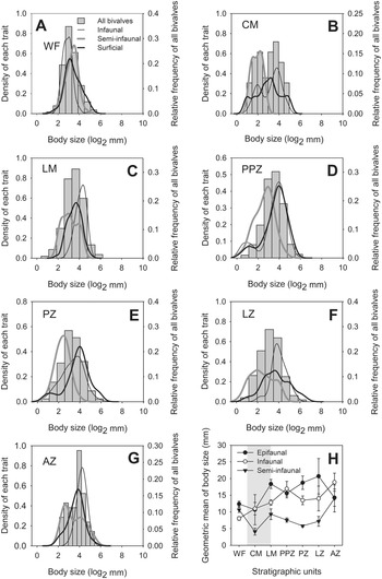
BSDs were highly variable between tiering categories and stratigraphic units, and only a third of BSDs were normally distributed (Fig. 6A–G, Supplementary Table 4). The BSDs of infaunal and semi-infaunal bivalves differed significantly in all stratigraphic units (K-S test: d = 0.51, p c < 0.01; Supplementary Table 5). The BSDs of semi-infaunal and epifaunal taxa were not significantly different from each other during the pre-extinction Westbury Formation and later postextinction Angulata Zone (K-S test: d = 0.27, p c > 0.01), whereas the infaunal and epifaunal BSDs had the same shapes during the Cotham Member, pre-Planorbis Zone, and Angulata Zone (K-S test: d = 0.209, p c > 0.01) (Supplementary Table 5). Only during the Langport Member and Planorbis Zone did all tiers have significantly different BSDs from one another (K-S test: d = 0.42, p c < 0.01; Supplementary Table 5).
Changes in the size–frequency distributions of the body sizes of infaunal, semi-infaunal, and epifaunal bivalves through the Triassic–Jurassic of the United Kingdom. A, Westbury Formation (WF); B, Cotham Member (CM; Lilstock Formation); C, Langport Member (LM; Lilstock Formation); D, pre-Planorbis Zone (PPZ); E, Planorbis Zone (PZ); F, Liasicus Zone (LZ); G, Angulata Zone (AZ). The fitting of each curve is based on a combination of kernel density estimation and smoothed bootstrap resampling using bin sizes of 0.25 on a log2 scale. All distributions are unimodal but with highly variable skewed frequency distributions. H, Changes in the weighted marginal geometric mean values (±SE) for each tier through time.

Dramatic changes in the shapes of the BSDs occurred during and soon after the extinction event (i.e., in the Cotham and Langport Members). For instance, between the Westbury Formation and Cotham Member, the BSDs of all tiers change from being slightly leptokurtic, right skewed, and not-normally distributed, to being mesokurtic with high dispersion (of ~36%), while epifaunal and semi-infaunal bivalves exhibit normal distributions (K-S test: d = 0.13, p c < 0.01) (Supplementary Tables 4, 5). During the Langport Member, the BSDs of the tiers were significantly different (d = 0.48, p c < 0.01) (Supplementary Table 5). In general, all the assemblages showed a higher kurtosis and a significantly lower coefficient of variation (~27%) compared with the Cotham Member assemblage (Supplementary Table 4).
In the lower Blue Lias Formation, from the pre-Planorbis Zone to the Liasicus Zone, BSDs tend to be mesokurtic, with a switch toward positive skews and with a progressive expansion of variance in all three tiers (Table 1). The Angulata Zone, however, records a contraction in the BSDs of all tiers by around ~18%. The BSDs of infaunal and epifaunal taxa record left-skewed distributions with high kurtosis (with mode ~4 log2 mm), while the BSD of semi-infaunal species is mesokurtic with a positive skew (Supplementary Table 4).
Significant differences were detected by GLMs between the mean body sizes of each tier (Wald χ2(2) = 53.29, p < 0.001). Epifaunal taxa recorded the largest mean size (15.7 ± 0.4 mm), infaunal taxa recorded intermediate mean sizes (12.4 ± 0.3 mm), and semi-infaunal bivalves recorded the smallest mean sizes (Fig. 6H, Supplementary Fig. 3). Although the GLMs did not find significant differences between the mean sizes of all bivalves from the Cotham Member (10.3 ± 0.2 mm) and Westbury Formation (8.5 ± 0.4 mm), both of those stratigraphic units record the smallest mean sizes in each section studied (Wald χ2(6) = 52.93, p < 0.05) (Supplementary Fig. 3, Supplementary Table 6). Bivalves from the Langport Member recorded a significant increase in size of ~30% (13.7 ± 0.2 mm) compared with those from the Cotham Member and Westbury Formation. Mean body size gradually increases from the Rhaetian Langport Member through the overlying Hettangian Blue Lias Formation, reaching an average size of 15.7 ± 0.3 mm in the Angulata Zone (Supplementary Fig. 3, Supplementary Table 6).
The mean body size of each mode of life significantly increases through the Triassic–Jurassic interval (Wald χ2(12)=153.96, p < 0.05) (Fig. 6H, Supplementary Table 6). However, during the extinction event, semi-infaunal bivalves are the only tier to record a significant decrease in mean body size; from 10.4 ± 0.4 mm in the Westbury Formation to 4.0 ± 0.4 mm in the Cotham Member. This decrease is probably due to there being only a single taxon, Modiolus sp., representing this mode of life in the extinction horizon.
Comparison with the Null Model
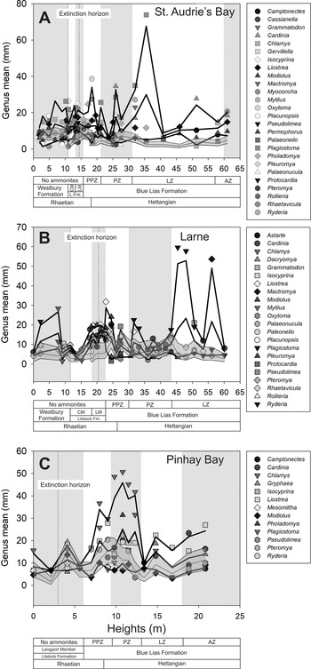
Comparison of the mean body size of each species per sample with the average curves from the null model shows that the bivalves record a significant directional trend toward larger body size through the study interval (Fig. 7, Table 3). This pattern is broadly consistent across the region, although there appears to be some variation at the local scale during the recovery: mean size in the St. Audrie's Bay section increases significantly in the late Liasicus Zone (35 m above base of measured section); at Larne, larger sizes are recorded from the early Liasicus Zone (at 45 m); while at Pinhay Bay, a significant expansion of body size is recorded during the pre-Planorbis Zone (at 7.5 m). In all cases, the expansion toward larger size was driven by genera such as Plagiostoma, Mactromya, Cardinia, Pholadomya, and Liostrea (Fig. 7A–C). Finally, although sizes were not significantly smaller than expected by chance during the extinction event, the recurrent overlap of the randomized and sampled data during the Cotham and Langport members does indicates a high occurrence of smaller-sized taxa during those units.
Contrasting null models of Triassic–Jurassic bivalve body size from St. Audrie's Bay (A), Larne (B), and Pinhay Bay (C). Each point represents the mean size of a specific genus recorded at the stratigraphic height shown (see Supplementary Data for detailed stratigraphic logs). Genus-level body sizes were plotted to avoid overcrowding of data points. Thick black lines show the average size of all individual bivalves from each sample, estimated from raw data, with 2.5% and 97.5% percentiles. The gray shaded area with thin black lines represents the null model, with 2.5% and 97.5% percentiles, calculated by row permutation (number of iterations = 9999) of the geometric mean of each individual by species through the samples. Key to stratigraphic units as in Fig. 3.

Observed and randomized mean body-size values for each Triassic–Jurassic section. Loc., locality; AB, St. Audrie's Bay; PB, Pinhay Bay; L, Larne, Northern Ireland. t-value, t-distribution value. Significance values: *p < 0.05; ***p < 0.001.

Discussion
Patterns of Change in Body Size during the Extinction and Recovery Event
Results indicate that the LTE simultaneously affected different localities, within the temporal resolution of the stratigraphic units analyzed. The BSDs of recorded bivalve species changed through the event and recovery, with a flattening of the BSD immediately after the LTE (Fig. 5A,B), followed by a narrowing of BSD and later rapid expansion of the body-size range during the recovery phase. The patterns of body-size changes recorded in this study resemble those recorded in studies of other extinction events (Payne Reference Payne2005; Morten and Twitchett Reference Morten and Twitchett2009; He et al. Reference He, Twitchett, Zhang, Shi, Feng, Yu, Wu and Peng2010; Rego et al. Reference Rego, Wang, Altiner and Payne2012; Martinez-Diaz et al. Reference Martinez-Diaz, Phillips, Nyborg, Espinosa, Tavora, Centeno-Garcia and Vega2016; Sigurdsen and Hammer Reference Sigurdsen and Hammer2016; Rita et al. Reference Rita, Natscher, Duarte, Weis and De Baets2019; Piazza et al. Reference Piazza, Duarte, Renaudie and Aberhan2019; Foster et al. Reference Foster, Gliwa, Lembke, Pugh, Hofmann, Tietje, Varela, Foster, Korn and Aberhan2020) and add new insights to previous studies of the LTE. For instance, Mander et al. (Reference Mander, Twitchett and Benton2008), Atkinson and Wignall (Reference Atkinson and Wignall2019, Reference Atkinson and Wignall2020), Atkinson et al. (Reference Atkinson, Wignall, Morton and Aze2019), and Wignall and Atkinson (Reference Wignall and Atkinson2020) reported changes in species composition between the Westbury Formation and Cotham Member (Lilstock Formation) and recorded an apparent reduction of body size of new arrivals and surviving taxa during the early recovery interval (i.e., the Langport Member). This study confirms the same changes during the extinction interval, although the changes in body size are complex.
The first extinction pulse, between the Westbury Formation and Cotham Member, was not size selective and so generated gaps across the BSD (Fig. 5B). In addition, the BSD of bivalve species in the Cotham Member has a negative skew due to the presence of surviving taxa that record a decrease in body size below the grand mean. These taxa include Isocyprina concentricum, Modiolus sp., Placunopsis alpina, and Mytilus cloacinus (Fig. 5B). Immediately after the extinction event (i.e., in the Langport Member), the variance of the BSD decreases significantly, because all recorded taxa cluster around the grand mean (Figs. 4B–D and 5A). In the overlying Blue Lias Formation, an expansion in size is recorded from the pre-Planorbis Zone, and the BSDs shift toward a positive skew due the occurrence of larger taxa during the recovery (Figs. 4D, 5A,B).
Similar increases in body size during the Early Jurassic recovery are also recorded from other studies in the United Kingdom and elsewhere. The trace fossils Thalassinoides, Diplocraterion, and Arenicolites show a substantial size increase from the Langport Member to the Angulata Zone in the southwest United Kingdom (Twitchett and Barras Reference Twitchett and Barras2004; Barras and Twitchett Reference Barras and Twitchett2007, Reference Barras, Twitchett, Mangano and Buatois2016). Ammonites that survived the LTE expanded their body size by more than 10% toward the top of the Hettangian (Dommergues et al. Reference Dommergues, Montuire and Neige2002). Studies at community level from sites within the United Kingdom confirm a progressive accumulation of larger bivalve taxa through the Blue Lias Formation (Mander et al. Reference Mander, Twitchett and Benton2008), and recent studies (Atkinson and Wignall Reference Atkinson and Wignall2019, Reference Atkinson and Wignall2020) confirm our observations, demonstrating that body-size increase is driven mainly by newly originated clades.
Similar size increases in marine animals during postextinction recovery intervals have been recorded for other extinction events. Following the end-Devonian mass extinction, crinoids exhibited significant body-size increase (Brom et al. Reference Brom, Salamon and Gorzelak2018). Conodonts exhibit significant increase in size and high disparity level after the Frasnian–Famennian crisis (Girard and Renaud Reference Girard and Renaud2012). Brachiopods, bivalves, gastropods, and trace fossils show a directional trend to larger sizes during the recovery after the late Permian mass extinction (Twitchett Reference Twitchett2007; Metcalfe et al. Reference Metcalfe, Twitchett and Price–Lloyd2011; Pietsch et al. Reference Pietsch, Petsios and Bottjer2016; Foster et al. Reference Foster, Danise, Price and Twitchett2017, Reference Foster, Danise, Price and Twitchett2018, Reference Foster, Gliwa, Lembke, Pugh, Hofmann, Tietje, Varela, Foster, Korn and Aberhan2020). Similar results were recorded by Rego et al. (Reference Rego, Wang, Altiner and Payne2012) with foraminifera from the late Permian to the Late Triassic. Cephalopods and bivalves recorded an increase in body size after the early Toarcian extinction event (Morten and Twitchett Reference Morten and Twitchett2009; Rita et al. Reference Rita, Natscher, Duarte, Weis and De Baets2019), and venerid bivalves recorded increases in body size after the Cretaceous/Paleogene (K/Pg) boundary (Lockwood Reference Lockwood2005).
The temporal trajectory of the body size of each species, expressed as residuals in this study, resembles the diffusion model in which all species move away from the lower bound or “small mean size” (see Figs. 1, 5B). This could represent a physiological optimum (Brown et al. Reference Brown, Marquet and Taper1993; McShea Reference McShea1994) wherein macroevolutionary forces such as extinction risk and selective advantage determine the length of the right and the left tail of the BSD, respectively (Clauset and Erwin Reference Clauset and Erwin2008), and constrain the upper and lower limits of a taxon's body size around a physiological optimum size.
Testing the Lilliput Effect Model
Twitchett (Reference Twitchett2007) and Harries and Knorr (Reference Harries and Knorr2009) described four potential and nonexclusive scenarios to explain why small-sized animals dominate fossil assemblages after extinction events: (1) the preferential survival of small taxa and/or selective extinction of large taxa; (2) the postextinction origination of many newly evolved lineages at small initial body size; (3) a potential bias in the preservation of larger taxa in the immediate extinction aftermath; and (4) the Lilliput effect sensu stricto of Urbanek (Reference Urbanek1993), whereby surviving taxa undergo temporary size reduction in the immediate aftermath of the extinction event. In the case of Triassic–Jurassic bivalves, our study shows that there was no size selection during the LTE, at least in the UK sections we studied. It appears that the LTE did not selectively eliminate larger or smaller taxa; rather, each body-size class had the same probability of extinction (Fig. 5B). During the extinction event (Cotham Member), the mean body size of the entire community did not change significantly compared with the pre-extinction Westbury Formation. However, the BSD remained highly platykurtic, because taxa were extirpated randomly with respect to body size, which resulted in a redistribution of species along the size axis (Fig. 5B). For instance, M. cloacinus, P. alpina, Modiolus sp., and I. concentricum record apparent dwarfism (i.e., the Lilliput Effect sensu stricto), three taxa record size increases (Pteromya crowcombeia, Cardinia regularis, and Chlamys valoniensis), two species do not record any changes (Rhaetavicula contorta and Protocardia rhaetica), and only one taxon (Pleuromya sp.) emerges at the upper side of the BSD (Fig. 5B).
Langport Member assemblages record a highly leptokurtic BSD with lower coefficient of variation immediately after the extinction, because the sizes of the survivors and victims were centered around the grand mean size, with a skew close to zero (see Figs. 4D, 5A). The clustering of species around the mean size immediately after the LTE (Langport Member) is influenced by the arrival of comparatively smaller species belonging to new clades, which could indicate the presence of environmental constraints on size. Subsequently, newly arriving taxa expand through morphospace by increasing their size, and larger taxa become more common, which extends the right tail of the BSD.
Thus, the size changes recorded in bivalves through the LTE in the UK sections studied appear to be caused by a combination of the Lilliput effect sensu stricto and the appearance of new, small-sized taxa in the extinction aftermath, and not by selective extinction. The BSD patterns observed during the Cotham and Langport members are also consistent with McKinney's (Reference McKinney and McNamara1990) suggestion that after a nonselective extinction event, the BSD changes to a flatter version of the pre-extinction BSD as result of an equal chance of extinction of each size class. Each size bin had the same probability of extinction, and so tails of the BSD may be more susceptible to disappear, because they contain proportionally fewer taxa. Finally, even though the mechanisms of body-size reduction were not evaluated here, several physiological responses to cope with warming events have been identified in some organisms. For instance, shifts in cell sizes, reduction of the metabolic rate, growth, and/or modification of life cycles (Atkinson Reference Atkinson, Begon and Fitter1994; Millien et al. Reference Millien, Kathleen Lyons, Olson, Smith, Wilson and Yom-Tov2006; Daufresne et al. Reference Daufresne, Lengfellner and Sommer2009; Forster et al. Reference Forster, Hirst and Atkinson2012; Hermaniuk et al. Reference Hermaniuk, van de Pol and Verberk2021; Verberk et al. Reference Verberk, Atkinson, Hoefnagel, Hirst, Horne and Siepel2021). Recently, Rita et al. (Reference Rita, Natscher, Duarte, Weis and De Baets2019) suggested that the high occurrence of juvenile belemnites during the Pliensbachian–Toarcian extinction event could be an ecophysiological response to cope with high temperatures. The faster maturity at smaller sizes could reduce the resource-dependent mortality and intraspecific competition in warm conditions (Sheridan and Bickford Reference Sheridan and Bickford2011; Forster et al. Reference Forster, Hirst and Atkinson2012; Le Bris et al. Reference Le Bris, Pershing, Gaudette, Pugh and Reardon2017; Verberk et al. Reference Verberk, Calosi, Brischoux, Spicer, Garland and Bilton2020, Reference Verberk, Atkinson, Hoefnagel, Hirst, Horne and Siepel2021). In this sense, we could expect a similar ecological signal for bivalves across the end-Triassic extinction, considering the similarity of the environmental drivers. However, further data are required to unravel the mechanisms that drove size changes through the end-Triassic hyperthermal event.
Potential Abiotic Factors and Timing of Recovery
Two questions arise regarding the trajectory of the body-size changes: (1) What drove the changes in bivalve body size during the recovery stage? (2) How does the rate of recovery recorded in our study compare with results from previous studies of the LTE? Regarding the potential drivers of size change, a number of studies have identified abiotic factors that could have driven body-size changes in marine organisms during past extinction events (Twitchett Reference Twitchett2007; Zhang and He Reference Zhang and He2008; Wade and Twitchett Reference Wade and Twitchett2009; He et al. Reference He, Shi, Yang, Zhang, Yue, Xiao, Wu, Chen and Wu2016) and in relation to present-day climate change (e.g., Daufresne et al. Reference Daufresne, Lengfellner and Sommer2009; Stige and Kvile Reference Stige and Kvile2017). The dissolved oxygen content of aquatic systems has been invoked as one of the main factors in structuring body size and species diversity at different temporal scales (Payne et al. Reference Payne, McClain, Boyer, Brown, Finnegan, Kowalewski, Krause, Lyons, McShea, Novack-Gottshall, Smith, Spaeth, Stempien and Wang2011; Riding et al. Reference Riding, Liang, Lee and Virgone2019; Rubalcaba et al. Reference Rubalcaba, Verberk, Hendriks, Saris and Woods2020).
Increases in oxygen levels through the Phanerozoic have had a strong control upon the ecological complexity of marine systems and the body size of marine taxa (Novack-Gottshall Reference Novack-Gottshall2008; Payne et al. Reference Payne, McClain, Boyer, Brown, Finnegan, Kowalewski, Krause, Lyons, McShea, Novack-Gottshall, Smith, Spaeth, Stempien and Wang2011), especially during environmental stress. For example, by using the relative abundance of the rare earth element cerium, which is a proxy for paleo-oxygenation of marine environments, He et al. (Reference He, Twitchett, Zhang, Shi, Feng, Yu, Wu and Peng2010) demonstrated that during the late Permian mass extinction event, the body size of brachiopods decreased strongly with increasing hypoxia. Similar size responses have been described for other taxa during extinction events that are associated with oceanic anoxic episodes: for example, Pliensbachian–Toarcian ammonites (Morten and Twitchett Reference Morten and Twitchett2009) and belemnites (Rita et al. Reference Rita, Natscher, Duarte, Weis and De Baets2019) and Permian–Triassic gastropods and bivalves (Metcalfe et al. Reference Metcalfe, Twitchett and Price–Lloyd2011). The burrow diameters of infaunal benthic marine macroinvertebrates also record similar changes through many past extinction events (Twitchett and Barras Reference Twitchett and Barras2004), including through the LTE (Barras and Twitchett Reference Barras and Twitchett2007).
The LTE was ultimately caused by a major episode of global warming due to CAMP eruptions, with a rise in atmospheric CO2 from ca. 750 to ca. 2000 ppmv and an increase of 3°C–4°C in mean seawater temperature (McElwain et al. Reference McElwain, Beerling and Woodward1999; Greene et al. Reference Greene, Martindale, Ritterbush, Bottjer, Corsetti and Berelson2012). Widespread hypoxia and anoxia are a predicted consequence of global warming due to lower dissolved oxygen concentrations in warmer seawater, weakness of thermohaline ocean circulation, increased likelihood of stratification, and shallowing of euxinic conditions (Kidder and Worsley Reference Kidder and Worsley2010; Breitburg et al. Reference Breitburg, Levin, Oschlies, Grégoire, Chavez, Conley, Garçon, Gilbert, Gutiérrez, Isensee, Jacinto, Limburg, Montes, Naqvi, Pitcher, Rabalais, Roman, Rose, Seibel, Telszewski, Yasuhara and Zhang2018). Jaraula et al. (Reference Jaraula, Grice, Twitchett, Böttcher, LeMetayer, Dastidar and Opazo2013) used biomarker evidence (e.g., the abundance of isorenieratane) to suggest that fluctuations between dysoxic, anoxic, and euxinic conditions could be one of the main factors constraining the post-LTE recovery phase. Oxygen concentration is only one of the major marine biogeochemical parameters predicted to change during warming events (Rubalcaba et al. Reference Rubalcaba, Verberk, Hendriks, Saris and Woods2020) but has the potential to trigger drastic physiological modifications in marine ectotherms (Sheridan and Bickford Reference Sheridan and Bickford2011; Rubalcaba et al. Reference Rubalcaba, Verberk, Hendriks, Saris and Woods2020; Verberk et al. Reference Verberk, Atkinson, Hoefnagel, Hirst, Horne and Siepel2021). Regarding the timescale, our study indicates that the extinction episode and the appearance of the first colonizers was faster than previously proposed (Thibodeau et al. Reference Thibodeau, Ritterbush, Yager, West, Ibarra, Bottjer, Berelson, Bergquist and Corsetti2016). However, recent studies performed by Weedon et al. (Reference Weedon, Page and Jenkyns2019) would assign to the Hettangian a longer duration (4.1 Myr) compared with previous observations (1.7–2 Myr) (Schaltegger et al. Reference Schaltegger, Guex, Bartolini, Schoene and Ovtcharova2008; Schoene et al. Reference Schoene, Guex, Bartolini, Schaltegger and Blackburn2010; Wotzlaw et al. Reference Wotzlaw, Guex, Bartolini, Gallet, Krystyn, McRoberts, Taylor, Schoene and Schaltegger2014) and cyclostratigraphy (Ruhl et al. Reference Ruhl, Deenen, Abels, Bonis, Krijgsman and Kurschner2010, Reference Ruhl, Hesselbo, Hinnov, Jenkyns, Xu, Riding, Storm, Minisini, Ullmann and Leng2016; Hüsing et al. Reference Hüsing, Beniest, van der Boon, Abels, Deenen, Ruhl and Krijgsman2014). This would suggest that recovery during the Hettangian was slower than previously indicated (Thibodeau et al. Reference Thibodeau, Ritterbush, Yager, West, Ibarra, Bottjer, Berelson, Bergquist and Corsetti2016; Lindström et al. Reference Lindström, Erlström, Piasecki, Nielsen and Mathiesen2017), whereby the ecological impact of the LTE requires a reevaluation.
The most current chronology of the biotic and abiotic events associated with the LTE establishes that CAMP activity began around the last occurrence of Choristoceras marshi (~201.52 ± 0.14 Ma) (Lindström et al. Reference Lindström, Erlström, Piasecki, Nielsen and Mathiesen2017), which coincides with the initial negative δ13Corg excursion, which had a duration of ~20–40 kyr (Ruhl et al. Reference Ruhl, Deenen, Abels, Bonis, Krijgsman and Kurschner2010). Thibodeau et al. (Reference Thibodeau, Ritterbush, Yager, West, Ibarra, Bottjer, Berelson, Bergquist and Corsetti2016) divides the composition changes of the marine fauna with respect to CAMP activity into two stages: first, the “extinction interval” that spans from C. crickmayi to the first occurrence of Psiloceras spelae, that is, the base of the Jurassic; and second, the “depauperate interval” that spans from P. spelae to the Kammerkarites Zone. In the UK succession, the first stage would equate to the interval spanning the Cotham Member to the Triassic/Jurassic boundary (i.e., in the pre-Planorbis Zone), and the second stage would span from the base of the Hettangian to the base of the Liasicus Zone (Fig. 2C).
Our data show that newly colonizing taxa begin to arrive during the Langport Member, and the BSDs increase significantly in variance in all localities (Fig. 5) before the Triassic/Jurassic boundary. Using the timescale of Ruhl et al. (Reference Ruhl, Deenen, Abels, Bonis, Krijgsman and Kurschner2010) and Ruhl and Kurschner (Reference Ruhl and Kurschner2011), this suggests that initial recovery in the United Kingdom had already begun by ca. 100–120 kyr after the extinction, that is, before peak warming and the depauperate interval of Thibodeau et al. (Reference Thibodeau, Ritterbush, Yager, West, Ibarra, Bottjer, Berelson, Bergquist and Corsetti2016) and while CAMP volcanism was still active. Several studies have shown that after the LTE, marine communities along the western coast of Pangea had lower diversity than those in Tethys (Damborenea et al. Reference Damborenea, Echevarría and Ros-Franch2013; Ritterbush et al. Reference Ritterbush, Bottjer, Corsetti and Rosas2014), although these apparent differences in recovery rates have not been explored in detail.
Our results agree with previous studies that have suggested that final recovery in the United Kingdom is reached in the late Hettangian (e.g., Barras and Twitchett Reference Barras and Twitchett2007; Mander et al. Reference Mander, Twitchett and Benton2008; Pugh et al. Reference Pugh, Danise, Brown and Twitchett2014; Atkinson and Wignall Reference Atkinson and Wignall2019, Reference Atkinson and Wignall2020; Atkinson et al. Reference Atkinson, Wignall, Morton and Aze2019). Although not sampled in this study, previous analyses have also demonstrated that the sizes of benthic marine invertebrates continued to increase into the early Sinemurian (e.g., Barras and Twitchett Reference Barras and Twitchett2007). The absolute rates of recovery and size change depend on estimates of the duration of the Hettangian stage. Most studies have concluded that the Hettangian lasted between 1.7 and 2 Myr (e.g., Ruhl et al. Reference Ruhl, Deenen, Abels, Bonis, Krijgsman and Kurschner2010, Reference Ruhl, Hesselbo, Hinnov, Jenkyns, Xu, Riding, Storm, Minisini, Ullmann and Leng2016; Hüsing et al. Reference Hüsing, Beniest, van der Boon, Abels, Deenen, Ruhl and Krijgsman2014; Gradstein et al. Reference Gradstein, Ogg, Schmitz and Ogg2020); although Weedon et al. (Reference Weedon, Page and Jenkyns2019) suggest a longer duration of 4.1 Myr. If correct, this would suggest that recovery during the Hettangian was significantly slower in absolute terms than previously suggested (Thibodeau et al. Reference Thibodeau, Ritterbush, Yager, West, Ibarra, Bottjer, Berelson, Bergquist and Corsetti2016; Lindström et al. Reference Lindström, Erlström, Piasecki, Nielsen and Mathiesen2017).
Selectivity
Although there is no clearcut phylogenetic signal associated with the body sizes of survivors or extirpated taxa, our data show that semi-infaunal bivalves were most strongly affected during the extinction event (recorded as a decrease in body size) (Fig. 6H, Supplementary Tables S4, S6). These results suggest that ecology was more important in determining the body size in surviving taxa than historical (phylogenetic) aspects. The lack of a phylogenetic signal in the sizes of surviving or extirpated taxa is consistent with the premise that there is no size-related selectivity during mass extinction, meaning that the loss of taxa from any hierarchical level is no different from what would be expected by chance (Jablonski and Raup Reference Jablonski and Raup1995; McRoberts and Newton Reference McRoberts and Newton1995). Variability in size-selective extinction has been reported commonly in bivalves (Lockwood Reference Lockwood2005; Smith and Roy Reference Smith and Roy2006; Rivadeneira and Marquet Reference Rivadeneira and Marquet2007); however, the lack a phylogenetic signal in our data could be explained by the low variance in size between taxonomic levels and/or simply because the LTE was not selective at different extirpation categories and taxonomic levels.
Selective extinction against infaunal taxa has also been reported from previous studies of the LTE (Kiessling et al. Reference Kiessling, Aberhan, Brenneis and Wagner2007) and other extinction events (Jablonski and Raup Reference Jablonski and Raup1995; Rivadeneira and Marquet Reference Rivadeneira and Marquet2007), and this study found that 55% (6 out of 11) of the infaunal taxa went extinct during the LTE compared with 43% (3 out of 7) of the epifaunal forms. However, as demonstrated by Mander and Twitchett (Reference Mander and Twitchett2008), infaunal suspension feeders are relatively poorly preserved through the extinction interval, particularly in the southwest United Kingdom, and so rock record bias may explain part of this apparent selectivity (Mander and Twitchett Reference Mander and Twitchett2008). When we decomposed the infaunal group into semi-infaunal and shallow-infaunal forms, we found that semi-infaunal bivalves appear to be more strongly affected by the extinction event (80%, 4 out of 5 genera), with Modiolus sp. the only survivor. This may explain why semi-infaunal bivalves record a platykurtic distribution and smallest size during the Cotham Member (Fig. 5B).
Of the 13 taxa that disappear between Cotham Member and Langport Member, 5 have completely aragonitic skeletons, 7 are aragonitic with low Mg-calcite, and just 1 taxon has purely calcitic skeletal mineralogy. There is, however, a strong link between life mode and mineralogy, with almost all infaunal and semi-infaunal bivalves recorded in the Triassic–Jurassic of the United Kingdom having aragonitic skeletons (Mander and Twitchett Reference Mander and Twitchett2008). While this likely explains the taphonomic bias in the infaunal record, it also means that it is not possible to determine whether mineralogy or life habit was most important in determining selectivity.
Several studies have hypothesized that the LTE was accompanied by a biocalcification crisis due to ocean acidification, as evidenced by the extinction of hypercalcified taxa, occurrences of skeletal structures with malformations, decreases in shell thickness, and the high abundance of noncalcareous disaster taxa with organic-walled structures (Kiessling et al. Reference Kiessling, Aberhan, Brenneis and Wagner2007; Hautmann et al. Reference Hautmann, Benton and Tomasovych2008; Crne et al. Reference Crne, Weissert, Gorican and Bernasconi2011). However, in their multivariate analysis of all available global data, Dunhill et al. (Reference Dunhill, Foster, Azaele, Sciberras and Twitchett2018) recently showed that calcification is not a strong predictor of extinction selectivity during the LTE and concluded that ocean acidification was not a major factor in the extinctions. Indeed, benthic mollusks are able to survive in surprisingly acidic conditions, and their shells record characteristic dissolution and repair features when affected by in vivo acidification (Garilli et al. Reference Garilli, Rodolfo-Metalpa, Scuderi, Brusca, Parrinello, Rastrick, Foggo, Twitchett, Hall-Spencer and Milazzo2015). The presence of such features in fossil mollusks would provide unequivocal evidence of acidified conditions, but thus far has not been reported from the Triassic–Jurassic record.
Taphonomic Effects and Biases within the Dataset
Taphonomic biases are known to affect the fossil record, and it is possible that changes in BSDs through time could be affected by several potential biases, such as lithology, preservation, and changing water depth (Behrensmeyer et al. Reference Behrensmeyer, Kidwell and Gastaldo2000; Holland Reference Holland2000; Hunt Reference Hunt2004). Mander and Twitchett (Reference Mander and Twitchett2008) documented in detail the preservational and facies changes affecting the bivalve record of the southwest UK Triassic–Jurassic successions. They also undertook a gap analysis at the genus level to assess the relative completeness of the same stratigraphic units that were sampled in this study and concluded that, in most cases, between 54% and 61% of the genera expected in each unit actually occurred as fossils, and only the pre-Planorbis Zone was substantially worse (recording only 41% of expected genera; Mander and Twitchett Reference Mander and Twitchett2008). In their analysis of different tiers, Mander and Twitchett (Reference Mander and Twitchett2008) indicates that infaunal suspension feeders have a relatively poor fossil record overall, but particularly through the extinction and in the pre-Planorbis Zone. In addition, epifaunal bivalves are relatively poorly represented in the Blue Lias Formation compared with the underlying Westbury and Lilstock formations; and semi-infaunal bivalves are better represented from the Planorbis Zone onward than in the underlying stratigraphic units (Mander and Twitchett Reference Mander and Twitchett2008).
Certainly, the pre-Planorbis Zone does not appear to be anomalous, in terms of body size, or in any of our comparative analyses of the entire fauna (Figs. 2–4, Supplementary Fig. S4). Indeed, if preservation acted as a significant factor constraining our observations, then we would not expect to have recorded BSDs with similar shapes to those reported in other marine communities (cf. Warwick Reference Warwick1984; Labra et al. Reference Labra, Hernandez-Miranda and Quinones2015) (see Fig. 3D). In addition, our data have filled in some of the gaps in ranges of several genera reported by Mander and Twitchett (Reference Mander and Twitchett2008). Thus, we are confident that our size data are robust, with respect to taphonomy, and the differences found between the null model and the raw body-size data through the Triassic–Jurassic (Fig. 6) capture a true ecological signal and are not artifacts of preservation bias.
In terms of changing lithofacies, the Cotham Member is much sandier than the other units, representing a much shallower depositional setting, and the Langport Member is more carbonate dominated than other units, representing a lagoonal or ramp setting (Hesselbo et al. Reference Hesselbo, Robinson and Surlyk2004; Mander and Twitchett Reference Mander and Twitchett2008). Although it is unlikely that lithofacies is biasing preservation, and hence diversity, through most of the study interval, it is possible that the depositional setting controls recorded body size in the Lilstock Formation. The relatively small size of the Cotham Member assemblage may be at least partially explained by the environment if, for example, salinity was lower due to greater freshwater influence in those more proximal settings (Wignall Reference Wignall2001; Hesselbo et al. Reference Hesselbo, Robinson and Surlyk2004; Warrington et al. Reference Warrington, Cope and Ivimey-Cook2008). If salinity was normal, then we might expect bivalve species in shallower marine settings to be larger (Hauton Reference Hauton2016). The presence of localized, small, patchy stromatolites within the Cotham Member at some locations in southwest United Kingdom, though not those sampled in this study, also likely indicates abnormal, schizohaline conditions or may reflect the postextinction expansion of stromatolites (Radley et al. Reference Radley, Twitchett, Mander and Cope2008). Evidence of fluctuating salinities has also been recorded at some horizons in the overlying Langport Member (Boomer et al. Reference Boomer, Duffin, Swift, Swift and Martill1999). Thus, the small size of Cotham Member bivalves (Figs. 4D, 5B) and the low coefficient of variation in Langport Member assemblages (Figs. 4B, 5A) seem to be due to an environmental (salinity?) control.
Relative water depths also vary between the study sites. The sections at Pinhay Bay, St. Audrie's Bay, and Larne represent a depth gradient, from inshore to offshore (Hesselbo et al. Reference Hesselbo, Robinson and Surlyk2004). Despite this gradient, however, changes in BSDs happen simultaneously at the different localities (Fig. 4A), suggesting that relative position on the shelf does not significantly affect the timing of recorded body-size changes and overall trends.
Local and global sea levels, and hence water depth, did not remain constant through the studied interval. If fossil richness and abundance of the fossil record are correlated with sea level (Mander and Twitchett Reference Mander and Twitchett2008; Holland Reference Holland2016), then covariation between body size and sea level could be expected. High-quality fossils (abundant and well preserved) would be expected during transgressive to early-highstand phases (e.g., the lower Westbury Formation, Langport Member, and lower pre-Planorbis Zone; Hesselbo et al. Reference Hesselbo, Robinson and Surlyk2004; Mander and Twitchett Reference Mander and Twitchett2008). Moderate quality fossils would be expected during the highstand phases (upper Westbury Formation), and poor fossil quality would likely be observed during late-highstand and regressive phases (i.e., the Cotham Member; Mander and Twitchett Reference Mander and Twitchett2008). The raw species richness and rarefaction analyses of the Cotham Member are potentially consistent with this (Fig. 3A,B). The significant increase in the mean body size of the bivalve community from the Langport Member to the Angulata Zone apparently occurred without significant change in either sea level or lithofacies (Supplementary Fig. S4), suggesting that other factors were shaping the BSD during the postextinction interval. Smaller sizes were recorded in the Westbury Formation and, in particular, in the Cotham Member (Supplementary Fig. S4), and a narrowing of the BSD was recorded during transgressive to early-highstand phases (Langport Member) (Fig. 3D, Supplementary Fig. S4).
Alternatively, the nature of the preservation processes, as time averaging and/or transport, could affect the shape of BSD (Fagerstrom Reference Fagerstrom1964; Mancini Reference Mancini1978). Preburial transportation of loose shells by strong currents, could constrain the BSD toward the accumulation of larger sizes or generation of leptokurtic distributions (Fagerstrom Reference Fagerstrom1964), as we see in the Langport Member, for instance. On the other hand, increased degree of time averaging/condensation could lead to a more platykurtic BSD (e.g., Hunt Reference Hunt2004), as was recorded at the Cotham Member. However, the relatively low-energy Bahamian type that prevailed during the deposition of the Cotham Member and the Langport Member (Hallam Reference Hallam1960; Radley Reference Radley2002; Hesselbo et al. Reference Hesselbo, Robinson and Surlyk2004) preclude the accumulation of large size and/or development of leptokurtic BSD in bivalves. Alternatively, the platykurtic BSD observed in the Cotham Member resulted in very short period of time (~20 kyr). (Ruhl et al. Reference Ruhl, Deenen, Abels, Bonis, Krijgsman and Kurschner2010, Reference Ruhl, Bonis, Reichart, Damste and Kurschner2011) in the disappearance of species and the size expansion–reduction of some survivor taxa, whereby the potential effect of time averaging does not seem to fit from the pattern observed in the Cotham Member. Thus, the pattern of change in the BSD recorded in this study represents a true paleoecological signal.
One clear sampling bias is apparent in our data from the Angulata Zone, which are evidently undersampled (Fig. 3B, Supplementary Fig. S4). The lowest richness and lowest variance in body size recorded from this stratigraphic unit could be related to the relatively low number of samples compared with other units. However, despite that bias, this study still records similar trends in bivalve body size as those recorded by Atkinson et al. (Reference Atkinson, Wignall, Morton and Aze2019). Thus, the sustained increase in body size recorded after the extinction event in the whole assemblage and in individual taxa is unlikely to be the result of sampling or taphonomic biases, especially given the nature of the Blue Lias Formation rock record (Mander and Twitchett Reference Mander and Twitchett2008) and the fact that similar increases are recorded in other taxa, such as trace fossils (Barras and Twitchett Reference Barras and Twitchett2007).
By sampling three locations in one region (northwest Europe), this study better represents the true changes in body size through the Triassic–Jurassic extinction and recovery interval than previous studies that have relied on single sites, and it also reduces the effects of variation between localities, species, and stratigraphic units. As noted by Bambach (Reference Bambach1977) and Novack-Gottshall (Reference Novack-Gottshall2008), comparison of size trends among phylogenetically and ecologically unrelated taxa living in the same habitat is an important and powerful test of ecosystem-level processes, because environmental changes will often affect entire communities of organisms in a similar manner. Our data show that taphonomic heterogeneity does not strongly affect the BSD patterns found here. Despite this, it is noted that random effects can be more influential when sample sizes are low (Novack-Gottshall Reference Novack-Gottshall2008).
Our study agrees with previous empirical and theoretical studies of body size (McKinney Reference McKinney and McNamara1990, Reference McKinney1997) and provides new knowledge of the dynamics of body-size change through the LTE and subsequent Early Jurassic recovery. Our results suggest that the LTE acted rapidly and synchronously on the marine bivalve fauna across multiple sites, decreasing taxic richness and strongly modifying the shape of body-size distributions. No significant phylogenetic, ecological, and/or size-selective signals were found. This nonselective extinction resulted in a negatively skewed and platykurtic BSD in the shallow-marine, nearshore Cotham Member, probably controlled at least in part by the local environment. In the overlying Langport Member, the BSD still shows a negative skew, with the body sizes of surviving and extinct taxa accumulated around the median size, recording a low coefficient of variation. Newly colonizing taxa were also small, with body sizes near that of the median (“rebound size”). Thereafter, recovery of body size was relatively rapid, and later in the Hettangian, when the environmental conditions improved, larger individuals were recorded, and so the right tail of the BSD extended significantly.
Acknowledgments
Data collection occurred during L.F.O.'s Ph.D. studies, supported by the Alβan Programme (the European Union Programme of High Level Scholarships for Latin America; scholarship no. E07D402767CL) and CONICYT, Beca de Doctorado en el Extranjero por Gestión Propia 2007, Postdoctoral CONICYT. In addition, L.F.O. thanks the Kowalewski lab, (Florida Museum of Natural History) where this article was produced, and Postdoctoral Fondecyt No. 3160191 (CONICYT, Chilean Government). L.F.O. thanks R. Rivadeneira and S. Danise for useful comments that improved the article and S. Abades for help building the null model. For their advice and help in the field, L.F.O. thanks K. Page, I. Erlander, A. Jeram, and M. Simms.
Data Availability Statement
Data available from the Dryad Digital Repository: https://doi.org/10.5061/dryad.3xsj3txhc.