1. Introduction
The interaction between surface waves and deformable structures lies at the heart of hydroelasticity, a field that merges fluid dynamics with structural mechanics to study the coupled response of elastic bodies in a hydrodynamic environment. In polar and subpolar regions, a floating ‘ice plate’, a term frequently used throughout this study that refers to continuous sea ice (Williams & Squire Reference Williams and Squire2007; Montiel & Squire Reference Montiel and Squire2017; Squire Reference Squire2020), is subject to dynamic loading from wave action, atmospheric forces and anthropogenic sources, leading to complex hydroelastic responses. Of particular importance is the scenario in which the ice plate is mechanically constrained by a vertical boundary, a configuration commonly encountered in coastal infrastructure, harbours and ice barriers, where the ice freezes onto rigid structures like harbour walls, piers or platforms (Williams & Squire Reference Williams and Squire2002; Sharapov & Shkhinek Reference Sharapov and Shkhinek2014; van der Stap, Nielsen & Hendrikse Reference van der Stap, Nielsen and Hendrikse2024). Over the time scale of short-period dynamic loading, such frozen-in contact produces a locally clamped interface that strongly restricts ice motion. Similar edge constraints also arise in ice-covered canals, fjords and artificial ice barriers designed for coastal protection (Beltaos Reference Beltaos2004; Løset & Marchenko Reference Løset and Marchenko2009; Pogorelova, Zemlyak & Kozin Reference Pogorelova, Zemlyak and Kozin2019; Ren, Wu & Li Reference Ren, Wu and Li2020; Yang, Wu & Ren Reference Yang, Wu and Ren2021).
Physically realistic configurations in which floating ice interacts with rigid vertical boundaries arise in both natural and engineered environments. Ice covers may become temporarily frozen (adfrozen) to harbour walls, offshore gravity-based platforms, wind-turbine monopiles, docking structures or steep rocky shorelines during periods of sustained low air temperatures, producing strong kinematic restraint at the ice–structure interface (Løset & Marchenko Reference Løset and Marchenko2009; Sharapov & Shkhinek Reference Sharapov and Shkhinek2014). Such frozen-in conditions are recognised in engineering practice and standards (e.g. ISO 19906), and have been documented for offshore structures in Arctic and sub-Arctic seas, as well as for freshwater ice in lakes and harbours. In freshwater systems, ice commonly freezes directly to rock or concrete shorelines, forming anchored ice covers capable of sustaining significant elastic stresses under wind- or wave-induced motion (Gold Reference Gold1994; Beltaos Reference Beltaos2004). Similar boundary conditions are routinely employed in laboratory ice-tank experiments, where ice is frozen to rigid side walls, and in glaciomechanics, where ice shelves are idealised as thin elastic plates clamped at the grounding line (Holdsworth & Glynn Reference Holdsworth and Glynn1978; Kalyanaraman et al. Reference Kalyanaraman, Bennetts, Lamichhane and Meylan2019; Bennetts, Liang & Pitt Reference Bennetts, Liang and Pitt2022; Liang, Pitt & Bennetts Reference Liang, Pitt and Bennetts2024).
Motivated by these settings, the present study investigates the hydroelastic response of a floating ice plate clamped to a vertical wall and subjected to oscillatory loading. While long-term clamping of sea ice in the open ocean may be disrupted by tidal motion and the formation of tide cracks, the present study focuses on short-duration, localised oscillatory forcing. Examples include dynamic loading generated by vehicles, snowmobiles, aircraft or stationary machinery operating on or near ice, where excitation occurs on time scales of seconds to minutes (Khabakhpasheva & Korobkin Reference Khabakhpasheva and Korobkin2021). Over these intervals, ice that is strongly bonded to a rigid boundary may respond elastically as if clamped, providing a meaningful limiting case of high kinematic restraint (Nelson & Phukan Reference Nelson and Phukan1988; Sharapov Reference Sharapov2023). The clamped-edge configuration therefore offers a physically motivated and practically useful framework for examining wave reflection, stress localisation and nonlinear strain amplification near rigidly constrained boundaries.
The clamped boundary condition employed here is an idealised representation of the ice–structure interface. It implies that both the ice deflection and its normal derivative vanish at the contact line, corresponding to zero relative displacement and rotation between the ice and the rigid boundary. Such an approximation is appropriate when adhesion between ice and the structure is strong, which typically occurs at sufficiently low air and surface temperatures, when the structure is much stiffer than the ice and the ice response remains predominantly elastic (Nelson & Phukan Reference Nelson and Phukan1988; van der Stap et al. Reference van der Stap, Nielsen and Hendrikse2024). Under these conditions, and for loading that is quasi-static or oscillatory over short durations, the characteristic time scale of forcing is shorter than that associated with creep relaxation or debonding, and the adhesion strength can exceed the tensile strength of the ice, preventing separation at the interface. Conversely, the clamped assumption is not expected to hold when temperatures approach the melting point, during rapid ice motion or impact loading, in the presence of ice-phobic or low-adhesion surface coatings, or under prolonged cyclic loading that may lead to progressive debonding (Azimi Dijvejin et al. Reference Azimi Dijvejin, Jain, Kozak, Zarifi and Golovin2022; Donadei et al. Reference Donadei, Koivuluoto, Sarlin, Niemelä-Anttonen, Varis and Vuoristo2022). It is likewise inappropriate in regimes dominated by cracking, crushing or plastic deformation, which lie outside the elastic framework adopted here. The present study therefore focuses on the elastic, short-time response of ice strongly restrained at a rigid boundary, for which the clamped condition provides a physically meaningful limiting case and a useful reference for assessing nonlinear hydroelastic effects.
Although linear theories based on thin elastic plate models coupled with potential flow have offered foundational insights into wave scattering and flexural-gravity wave propagation beneath ice (Nevel Reference Nevel1958; Schulkes & Sneyd Reference Schulkes and Sneyd1988; Squire et al. Reference Squire, Hosking, Kerr and Langhorne1996), they inherently neglect nonlinear interactions that become crucial near flexural-gravity (hydroelastic) wave resonance, where the forced primary wave motion nonlinearly self-interacts. This harmonic resonance leads to the excitation of flexural-gravity waves at twice the primary frequency and wavelength, a condition not captured by linear models (Fox & Squire Reference Fox and Squire1994), and can result in secular terms in the perturbation expansion that manifest as unbounded growth in the second-order solution (Vanden-Broeck & Părău Reference Vanden-Broeck and Părău2011; Teng et al. Reference Teng, Liang, Gou, Korobkin and Malenica2020; Liang, Teng & Gou Reference Liang, Teng and Gou2022; Pambela et al. Reference Pambela, Ma, Maeda and Iijima2023).
This omission is particularly critical for the scenario of a wall-attached ice plate subject to localised loading, which is related to practical problems in ice-related seismology near rocks and shorelines. For instance, linear theory may underestimate fatigue damage and crack initiation at the base of offshore wind turbine monopiles in ice-covered waters, or mispredict the failure of landfast ice near rocky shorelines due to resonant forcing from repeated wave impacts or vehicle traffic (Høyland et al. Reference Høyland2021; Braun et al. Reference Braun, Dörner, Ter Veer, Willems, Seidel, Hendrikse, Høyland, Fischer and Ehlers2022). Unlike freely floating plates, wall-attached ice plates experience asymmetries in stress distribution and altered modal behaviour due to boundary-imposed constraints (Brocklehurst, Korobkin & Părău Reference Brocklehurst, Korobkin and Părău2010; Korobkin, Părău & Vanden-Broeck Reference Korobkin, Părău and Vanden-Broeck2011). When such a system is excited by oscillatory external loads such as stationary vehicles (e.g. snowmobiles, aircraft) or operational forces (e.g. construction equipment, vibrating machinery, wave impacts), the combination of localised forcing and boundary reflection strongly excites the system near its resonant frequencies. This is a fundamental and physically relevant nonlinear phenomenon that cannot occur in an infinite domain. The resulting nonlinear hydroelastic response leads to pronounced strain concentrations that are not uniformly distributed, with peaks emerging near the point of load application. These effects, which linear theory fails to predict, are of direct relevance to ice failure prediction and design of coastal and offshore infrastructure in cold regions (Høyland et al. Reference Høyland2021; Braun et al. Reference Braun, Dörner, Ter Veer, Willems, Seidel, Hendrikse, Høyland, Fischer and Ehlers2022).
Recent research has increasingly highlighted the importance of incorporating higher-order geometric nonlinearities into hydroelastic models. This need is amplified by the ongoing thinning of polar ice due to climate change and the rising levels of human activity in ice-covered marine environments (Timco & Weeks Reference Timco and Weeks2010; Selivanova, Iovino & Cocetta Reference Selivanova, Iovino and Cocetta2024). While material nonlinearity is indeed significant over long time scales, this study focuses on the short-term, dynamic response to oscillatory loading, where the large-deflection, geometric nonlinearity of the ice plate and the associated nonlinear fluid flow dominate the initial response. This approach provides a necessary first step before incorporating more complex material models. Nonlinear effects arising from geometric nonlinearity, fluid–structure interaction and intermodal coupling can profoundly influence strain localisation, stress magnitudes and the mechanisms governing wave-induced responses in ice plates. Nevertheless, the second-order behaviour of wall-attached ice covers remains relatively underexplored. Notable contributions include the extension of the plate Green’s function method to second-order problems by Hegarty & Squire (Reference Hegarty and Squire2008), and the work of Iijima & Ma (Reference Iijima and Ma2019), who investigated nonlinear wave behaviour along very large floating structures (VLFS) and identified a critical frequency at which the second-order wave amplitude grows considerably. Teng et al. (Reference Teng, Liang, Gou, Korobkin and Malenica2020) examined the reflection of second-order flexural–gravity waves from a vertical wall using an eigenfunction expansion technique, demonstrating that these waves can become unbounded at specific frequencies. Liang et al. (Reference Liang, Teng and Gou2022) employed both the plate Green’s function method and a higher-order boundary element method to assess the influence of plate length on second-order hydroelastic responses. In addition, Pambela et al. (Reference Pambela, Ma, Maeda and Iijima2023) conducted both analytical and experimental studies on nonlinear deflection waves propagating along a thin elastic plate floating on the water surface, further underscoring the significance of nonlinear effects in hydroelastic systems.
As introduced earlier, vertical boundaries play a pivotal role in modulating hydroelastic wave interactions and the resulting strain distribution within floating ice covers. These boundaries introduce reflection and interference phenomena, which lead to complex spatial variations in wave amplitude and associated mechanical responses. Investigations by Brocklehurst et al. (Reference Brocklehurst, Korobkin and Părău2010), Bhattacharjee & Soares (Reference Bhattacharjee and Soares2012) and Korobkin, Malenica & Khabakhpasheva (Reference Korobkin, Malenica and Khabakhpasheva2018) examined wave scattering by ice plates attached to vertical walls, demonstrating the critical influence of boundary conditions on the resulting wave field. Their findings revealed that ice clamping imposes a constraint on the incident wave amplitude to ensure that the strain in the ice plate remains below its critical yield, particularly at the point of attachment, where the strain is maximal. As a result, the permissible wave amplitude is significantly reduced compared with unclamped scenarios. The studies also showed that clamping modifies the deflection profile of the ice plate, causing the first peak, closest to the wall, to be the smallest. Building on this, Kalyanaraman et al. (Reference Kalyanaraman, Meylan, Bennetts and Lamichhane2020) and Meylan et al. (Reference Meylan, Ilyas, Lamichhane and Bennetts2021) explored wave reflection and mode trapping in ice shelves with fixed vertical boundaries, showing that linear flexural–gravity resonances can lead to large displacements at specific frequencies. These linear resonances are distinct from the nonlinear second-order resonances discussed later in this work. More recently, Bennetts, Williams & Porter (Reference Bennetts, Williams and Porter2024) analysed the strain field in a semi-infinite ice shelf using the thin plate approximation and reported that wave-induced strains are notably higher at low forcing frequencies. Together, these studies emphasise the need for accounting boundary-induced nonlinear amplification when evaluating the structural integrity and failure risk of ice-covered ocean environments.
The present study builds on the foundational work of researchers such as Squire et al. (Reference Squire, Hosking, Kerr and Langhorne1996), who pioneered the study of wave–ice interactions, and Fox & Squire (Reference Fox and Squire1994), who developed early models of hydroelastic vibrations in ice plates. More recent contributions by Bennetts, Biggs & Porter (Reference Bennetts, Biggs and Porter2007), Brocklehurst et al. (Reference Brocklehurst, Korobkin and Părău2010) and Hossain & De (Reference Hossain and De2024) have advanced our understanding of ice plate dynamics, particularly in the context of wave propagation and scattering. However, these studies have largely focused on linear effects, leaving a critical gap in our understanding of how nonlinearities influence the hydroelastic response of ice covers near rigid boundaries. This gap is particularly relevant for engineering applications, where accurate predictions of stress concentrations and fracture formation are essential for structural design and risk assessment. While ice exhibits complex viscoelastic and rate-dependent behaviour, this study employs an elastic plate model to isolate the fundamental role of geometric and fluid dynamic nonlinearities, a necessary first step before introducing material complexity. This approach is justified for the short-duration, dynamic forcing considered here, where the instantaneous elastic response is the primary driver of initial strain localisation and potential fracture initiation.
This work seeks to address the identified gaps by investigating the hydroelastic response of an ice plate clamped to a vertical wall under external pressure. The problem is formulated using nonlinear thin plate theory coupled with nonlinear water wave theory. To explore the influence of nonlinearity, second-order corrections to ice response are obtained. These corrections arise due to nonlinear interactions between the ice plate deflection and the hydrodynamic forces. The presence of a vertical wall introduces additional complexity, as wave reflection and diffraction significantly alter the pressure distribution on the ice plate. The problem is initially formulated for a general form of the external pressure distribution, allowing the model to capture a broad spectrum of realistic loading conditions. However, further analysis focuses on a specific case involving an oscillating point pressure, which serves as a fundamental representation of localised loading effects. A primary objective is to determine whether nonlinearity mitigates or amplifies stress concentrations in the ice plate. Previous research on second-order wave interactions with floating bodies has shown that nonlinear effects can either intensify or redistribute stresses, leading to different structural responses (Faltinsen Reference Faltinsen1993; Liu & Yue Reference Liu and Yue1998; Hegarty & Squire Reference Hegarty and Squire2008). The present study extends this understanding to ice-covered waters, revealing conditions under which second-order hydroelastic effects enhance or reduce stress levels. The influence of boundary constraints and localised forcing on the nonlinear wave field is central to this analysis.
The remainder of this paper is organised as follows. Section 2 presents the mathematical formulation of the governing equations and boundary conditions. Section 3 outlines the perturbation approach for obtaining the linear and second-order solutions. Section 4 provides a detailed discussion of the results and implications of nonlinear effects. Finally, § 5 summarises the key findings and outlines potential directions for future research.
2. Problem formulation
This study explores weakly nonlinear effects, focusing specifically on those up to the second order. The challenge lies in determining how to introduce nonlinearity into the problem, which can be achieved through three feasible avenues: incorporation within the plate equation, within the fluid layer or a combination of both. These avenues yield three distinct scenarios: a nonlinear plate coupled with nonlinear flow, a linear plate coupled with nonlinear flow and a nonlinear plate coupled with linear flow. However, it will be demonstrated later that within the framework of a weakly nonlinear perturbation analysis, based on small-amplitude forcing, with spatial and temporal variations occurring on the characteristic scales of the problem, and a thin elastic plate assumption, the nonlinearities inherent in the plate equation are negligible for the second-order solution. Consequently, employing a linear plate equation works well for investigating second-order problems. As a result, the contribution stemming from nonlinearity is solely attributed to the fluid equations.
Schematic of an ice-covered water domain of finite depth
 $H^\prime$
, with the left edge of the ice clamped to a rigid vertical wall and subjected to external pressure. Note that the ice draft (submerged portion) is not shown to scale.

We investigate the two-dimensional problem of hydroelastic vibrations of a semi-infinite ice plate clamped to a vertical wall and subjected to an external pressure forcing. While the governing equations are formulated for a general external pressure distribution, the subsequent analysis is specialised to an oscillating point load. A Cartesian coordinate system
 $(x^{\prime },y^{\prime })$
is such that the
 $x^\prime\text{-}$
axis,
 $y^\prime =0,\,$
 $x^{\prime }\gt 0,$
corresponds to the ice/water interface at equilibrium and
 $x^{\prime }=0$
to the vertical rigid wall, where
 $-H^{\prime } \lt y^{\prime } \lt 0$
, with
 $H^{\prime }$
as the uniform water depth, see figure 1. A prime stands for dimensional variables. The deflection of the ice plate, which is modelled as a thin elastic plate, is described by the equation
 $y^\prime = w^{\prime } (x^{\prime }, t^{\prime } )$
. The problem is formulated under the assumptions of potential flow with the velocity potential
 $\phi ^{\prime } (x^{\prime }, y^{\prime }, t^{\prime } )$
. The velocity potential satisfies
Laplace’s equation,
 \begin{equation} {\nabla} ^{2} \phi ^{\prime }\left (x^{\prime }, y^{\prime }, t^{\prime } \right )=0 \quad (-H^{\prime } \leqslant y^{\prime } \leqslant w^{\prime }\left (x^{\prime }, t^{\prime }\right ), \ \ x^{\prime } \gt 0), \end{equation}
the kinematic condition on the ice/water interface,
 \begin{equation} \frac {\partial w^{\prime }}{\partial t^{\prime }}=\frac {\partial \phi ^{\prime }}{\partial y^{\prime }}-\frac {\partial \phi ^{\prime }}{\partial x^{\prime }} \frac {\partial w^{\prime }}{\partial x^{\prime }} \quad (y^{\prime }=w^{\prime }\left (x^{\prime }, t^{\prime }\right ), \ \ x^{\prime } \gt 0), \end{equation}
a dynamic condition which follows from the thin plate equation and the Bernoulli equation for the hydrodynamic pressure,
 \begin{align} D \left [ \frac {1}{\sqrt {1+w_{x^{\prime }}^{\prime 2}}} \frac {\partial }{\partial x^{\prime }}\left [\frac {1}{\sqrt {1+w_{x^{\prime }}^{\prime 2}}} \frac {\partial }{\partial x^{\prime }}\left (\frac {w_{x^{\prime } x^{\prime }}^{\prime }}{\left (1+w_{x^{\prime }}^{\prime }\right )^{3 / 2}}\right )\right ]+\frac {1}{2}\left (\frac {w_{x^{\prime } x^{\prime }}^{\prime }}{\left (1+w_{x^{\prime }}^{\prime 2}\right )^{3 / 2}}\right )^{3}\right ] + M \frac {\partial ^{2} w^{\prime }}{\partial t^{\prime 2}} \\ \nonumber =-\rho g w^{\prime } -\rho \frac {\partial \phi ^{\prime }}{\partial t^{\prime }}-\frac {\rho }{2}\left (\boldsymbol{\nabla }\phi ^{\prime }\right )^{2} -p_{\textit{ext}}^{\prime }\left (x^{\prime }, t^{\prime }\right ) \quad \quad \big(y^{\prime }=w^{\prime } (x^{\prime }, t^{\prime } ), \ \ x^{\prime } \gt 0\big), \end{align}
where
 $D$
and
 $M$
are the flexural rigidity and mass per unit area of the ice plate, respectively. Note that the nonlinearity on the left-hand side of the plate (2.3) comes from the Cosserat model (Plotnikov & Toland Reference Plotnikov and Toland2011) of thin elastic plates. The right-hand side of (2.3) consists of the hydrodynamic pressure and a given external pressure
 $p_{\textit{ext}}^{\prime } (x^{\prime }, t^{\prime } )$
. The hydrodynamic pressure is related to the velocity potential by the Bernoulli equation, where
 $\rho$
is the water density and
 $g$
is the gravitational acceleration. Other conditions include the edge conditions at the vertical wall,
 \begin{equation} w^{\prime }=0, \ \ w_{x^{\prime }}^{\prime }=0 \quad \big(x^{\prime }=0, \ \ t^\prime \geqslant 0\big), \end{equation}
the no flow condition across the vertical wall,
 \begin{equation} \frac {\partial \phi ^{\prime }}{\partial x^{\prime }}=0 \quad \big(x^{\prime }=0, \ \ -H^{\prime } \leqslant y^{\prime } \leqslant 0\big), \end{equation}
and the no flow condition across the flat bottom,
 \begin{equation} \frac {\partial \phi ^{\prime }}{\partial y^{\prime }}=0 \quad \big(y^{\prime }=-H^{\prime }, \ \ x^{\prime }\gt 0\big). \end{equation}
Initially
 $(t^{\prime } = 0)$
, both the ice plate and the fluid are at rest,
 \begin{equation} w^{\prime }(x^{\prime },0) = w^{\prime }_{t^{\prime }}(x^{\prime },0) = 0, \quad \phi ^{\prime }\big (x^{\prime }, y^{\prime }, 0 \big ) = 0, \end{equation}
with
 $p_{\textit{ext}}^{\prime } (x^{\prime }, 0 ) = 0.$
Within the initial value problem starting from the rest, the ice deflection
 $w^{\prime }(x^{\prime },t^\prime )$
and the velocity potential
 $\phi ^{\prime }(x^{\prime },y^\prime , t^\prime )$
decay as
 $x^\prime \to \infty$
at any time instant.
The problem is formulated in the dimensionless variables,
 \begin{equation} \begin{aligned} x^{\prime }&=L x, \quad y^{\prime }=L y, \quad t^{\prime }=T \ t, \quad T=\sqrt {\frac {L}{g}}, \\ p_{\textit{ext}}^{\prime } \big(x^{\prime }, t^{\prime }\big)&=p_{\textit{sc}} \ p_{\textit{ext}}(x, t), \\ w^{\prime } \big(x^{\prime }, t^{\prime }\big)&=w_{s c} \ w(x, t)=\frac {p_{\textit{sc}}}{\rho g} \ w(x, t), \\ \phi ^{\prime } \big(x, y^{\prime }, t^{\prime }\big)&=\phi _{s c} \ \phi (x, y, t)=\frac {w_{s c} L}{T} \ \phi (x, y, t)=w_{s c} \sqrt {g L} \ \phi (x, y, t), \end{aligned} \end{equation}
where
 $p_{\textit{sc}}$
is the known pressure scale,
 $p_{\textit{ext}}(x,t)$
is the dimensionless function describing the shape and time evolution of the external pressure, and
 $L = ({D}/{\rho g} )^{1 / 4}$
is the characteristic length of the ice plate, see Squire et al. (Reference Squire, Hosking, Kerr and Langhorne1996). The dimensionless variables are represented by the same symbols without primes.
The kinematic condition (2.2) reads in the non-dimensional variables,
 \begin{align} \frac {\partial w}{\partial t}=\frac {\partial \phi }{\partial y}-\varepsilon \frac {\partial \phi }{\partial x} \frac {\partial w}{\partial x} \quad \quad (y=\varepsilon w(x, t), \ \ x\gt 0), \end{align}
where
 $\varepsilon =w_{s c}/L = p_{s c}/(\rho g L)$
is a small parameter of the problem.
Similarly, the dynamic condition (2.3) in the dimensionless variables takes the form
 \begin{align} \frac {1}{\sqrt {1+\varepsilon ^{2} w_{x}^{2}}} \frac {\partial }{\partial x}\left [\frac {1}{\sqrt {1+\varepsilon ^{2} w_{x}^{2}}} \frac {\partial }{\partial x}\left (\frac {w_{x x}}{\left (1+\varepsilon ^{2} w_{x}^{2}\right )^{3 / 2}}\right )\right ]+\frac {\varepsilon ^{2}}{2} \left (\frac {w_{x x}}{\left (1+\varepsilon ^{2} w_{x}^{2}\right )^{3 / 2}}\right )^{3} \\ \nonumber +\, \alpha \frac {\partial ^{2} w}{\partial t^{2}}=-w-\frac {\partial \phi }{\partial t}-\frac {\varepsilon }{2}(\boldsymbol{\nabla }\phi )^{2}-p_{\textit{ext}}(x, t) \quad \quad (y=\varepsilon w(x, t), \ \ x\gt 0), \end{align}
where
 $\alpha =M/(\rho L)=(\rho _{i} h_{i})/(\rho L)$
,
 $\rho _{i}$
is the ice density and
 $h_{i}$
is the ice thickness.
The boundary conditions (2.9) and (2.10) are approximated using series expansions of each term in them around
 $y=0$
, retaining terms up to
 $O (\varepsilon )$
as
 $\varepsilon \to 0$
. We obtain
 \begin{equation} w_{t}=\phi _{y}-\varepsilon \left (w \phi _{x}\right )_{x}+O \big(\varepsilon ^{2}\big ) \quad \quad (y=0, \ \ x\gt 0). \end{equation}
Correspondingly, the condition (2.10) provides
 \begin{equation} \frac {\partial ^{4} w}{\partial x^{4}}+\alpha \frac {\partial ^{2} w}{\partial t^{2}}+w+p_{\textit{ext}}(x,t)=-\phi _{t}-\varepsilon \!\left (w \phi _{t y}+\frac {1}{2}(\boldsymbol{\nabla }\phi )^{2}\! \right )+O \big(\varepsilon ^{2}\big) \!\quad\! (y=0, \ \ x\gt 0). \end{equation}
Therefore, the nonlinearity on the left-hand side of (2.10) can be neglected with the accuracy
 $O (\varepsilon ^{2} )$
as
 $\varepsilon \to 0$
. This implies that the plate can be treated as linear within the second-order approximation. The structural nonlinearity is important for higher-order problems where terms of order
 $O (\varepsilon ^{2} )$
and higher matter (Hegarty & Squire Reference Hegarty and Squire2008; Iijima & Ma Reference Iijima and Ma2019).
The plate deflection
 $w(x,t)$
and the velocity potential
 $\phi (x,y,t)$
are sought in the form
 \begin{align} w(x, t) & =w^{(1)}(x, t)+\varepsilon w^{(2)}(x, t)+O\big (\varepsilon ^{2}\big ), \end{align}
 \begin{align} \phi (x, y, t)& =\phi ^{(1)}(x, y, t)+\varepsilon \phi ^{(2)}(x, y, t)+O\big (\varepsilon ^{2}\big ) \end{align}
for
 $\varepsilon \to 0$
. All unknown functions
 $w^{(1)}, w^{(2)}, \phi ^{(1)}$
and
 $\phi ^{(2)}$
, and their spatial and temporal derivatives are assumed to remain order one with respect to the perturbation parameter
 $\varepsilon$
, ensuring that the asymptotic series are well ordered. The dimensionless parameter
 $\alpha ,$
which is small within the theory of thin elastic plates and independent of the linearisation parameter
 $\varepsilon ,$
is taken to be of order
 $O(1)$
in the present analysis. This assumption corresponds to the regime
 $\alpha \gg \varepsilon$
, or equivalently
 $p_{\textit{sc}} \ll \rho _i g h_i$
. If this inequality is not satisfied, the parameter
 $\alpha$
may be set to zero in the leading-order approximation.
By substituting (2.13) and (2.14) in the Laplace equation (2.1), the boundary conditions (2.11), (2.12), (2.4)–(2.7), and collecting terms with like powers of
 $\varepsilon$
, we arrive at the leading order problem with respect to
 $w^{(1)}(x,t)$
and
 $\phi ^{(1)} (x, y, t )$
,
 \begin{align} {\nabla} ^{2} \phi ^{(1)}\left (x, y, t \right )=0 \quad & \left ( -H \leqslant y \leqslant 0, \ \ x \gt 0 \right ),\\[-30pt]\nonumber\end{align}
 \begin{align} w_{t}^{(1)} =\phi _{y}^{(1)} \quad& \left ( y=0, \ \ x\gt 0 \right ),\\[-30pt]\nonumber\end{align}
 \begin{align} w_{x x x x}^{(1)}+\alpha w_{t t}^{(1)}+w^{(1)}+p_{\textit{ext}}(x,t)&=-\phi _{t}^{(1)}(x,0,t) \quad \left ( y=0, \ x\gt 0 \right ),\\[-30pt]\nonumber\end{align}
 \begin{align} w^{(1)}(0,t)=0, \ \ w_{x}^{(1)}(0,t)=0 \quad& \left ( t \geqslant 0 \right ),\\[-30pt]\nonumber\end{align}
 \begin{align} \frac {\partial \phi ^{(1)}}{\partial x}=0 \quad& \left (x=0, \ \ -H \leqslant y \leqslant 0\right ),\\[-30pt]\nonumber\end{align}
 \begin{align} \frac {\partial \phi ^{(1)}}{\partial y}=0 \quad& \left ( y=-H, \ \ x\gt 0\right ),\\[-30pt]\nonumber\end{align}
 \begin{align} w^{(1)}(x,0) = w^{(1)}_t(x,0) = 0, \quad& \phi ^{(1)}(x,y,0) = 0,\\[-30pt]\nonumber\end{align}
 \begin{align} w^{(1)} \to 0, \quad& \phi ^{(1)} \to 0 \quad \text{ as }\quad x \to \infty ,\end{align}
where
 $H = H^{\prime }/L$
is the dimensionless water depth.
Correspondingly, collecting the terms proportional to
 $\varepsilon$
, we arrive at the second-order problem with respect to
 $w^{(2)}(x,t)$
and
 $\phi ^{(2)} (x, y, t )$
,
 \begin{align} {\nabla} ^{2} \phi ^{(2)}\left (x, y, t \right )=0 \quad& \left ( -H \leqslant y \leqslant 0, \ \ x \gt 0 \right ),\\[-30pt]\nonumber\end{align}
 \begin{align} w_{t}^{(2)} =\phi _{y}^{(2)}-\left (w^{(1)} \phi _{x}^{(1)}\right )_{x} \quad & \left ( y=0, \ x\gt 0 \right ),\\[-30pt]\nonumber\end{align}
 \begin{align} w_{x x x x}^{(2)}+\alpha w_{t t}^{(2)}+w^{(2)}=-\phi _{t}^{(2)} &- \left \{w^{(1)} w_{t t}^{(1)}+\frac {1}{2}\left (w_{t}^{(1)}\right )^{2}+\frac {1}{2}\left (\phi _{x}^{(1)}\right )^{2}\right \} \!\quad\! \left ( y=0, \ x\gt 0 \right ),\end{align}
 \begin{align} w^{(2)}(0,t)=0, \ \ & w_{x}^{(2)}(0,t)=0 \quad \left ( t \geqslant 0 \right ),\\[-30pt]\nonumber\end{align}
 \begin{align} \frac {\partial \phi ^{(2)}}{\partial x}=0 \quad & \left ( x=0, \ \ -H \leqslant y \leqslant 0 \right ),\end{align}
 \begin{align} \frac {\partial \phi ^{(2)}}{\partial y}=0 \quad & \left ( y=-H, \ \ x\gt 0 \right ),\\[-30pt]\nonumber\end{align}
 \begin{align} w^{(2)}(x,0) = w^{(2)}_t(x,0) = 0, \quad & \phi ^{(2)}(x,y,0) = 0,\\[-30pt]\nonumber\end{align}
 \begin{align} w^{(2)} \to 0, \quad & \phi ^{(2)} \to 0 \quad \text{ as }\quad x \to \infty.\end{align}
It is noteworthy that the second-order problem (2.23)–(2.30) is similar to the leading order problem (2.15)–(2.22), but with a fictitious external pressure
 \begin{equation} p_{\textit{ext}}^{(2)}(x,t)=w^{(1)} w_{tt}^{(1)}+\frac {1}{2}\left (w_{t}^{(1)}\right )^{2}+\frac {1}{2}\left (\phi _{x}^{(1)}\right )^{2} \end{equation}
and extra forcing in the kinematic boundary condition (2.24).
We consider
 $p_{{ext}}(x,t)$
to be time periodic with a dimensionless frequency
 $\omega$
,
 \begin{equation} p_{\textit{ext}}(x,t)={\textrm{Re}}\,\left \{P_{\textit{ext}}(x) \ \textrm{e}^{-\textrm{i} \omega t}\right \}, \end{equation}
where
 $P_{\textit{ext}}(x)$
is a given dimensionless function. The dimensional frequency is
 $\omega ^{\prime } = \omega \sqrt {g/L}$
. This time-harmonic form does not satisfy the homogeneous initial condition
 $p_{\textit{ext}}(x,0)=0$
, as it represents the forcing for the steady-state, time-periodic response. In the present study, we limit ourselves to the steady-state solution, which corresponds to the limit as
 $t \to \infty$
after the decay of initial transients. Consequently, the precise form of the transient adjustment and, hence, of the forcing function that would satisfy the initial condition, has no influence on the steady-state solution of interest. The far-field conditions (2.22) and (2.30) are replaced with the condition that the steady-state solutions contain no incident waves as
 $x \to \infty$
.
Then, the solution of the leading order problem (2.15)–(2.22) is sought in the form
 \begin{align} w^{(1)}(x, t) & ={\textrm{Re}}\,\left \{W^{(1)}(x) \ \textrm{e}^{-\textrm{i} \omega t}\right \}, \end{align}
 \begin{align} \phi ^{(1)}(x, y, t) & ={\textrm{Re}}\,\left \{\left ( -\textrm{i} \omega \right ) \varphi ^{(1)}(x, y) \ \textrm{e}^{-\textrm{i} \omega t}\right \}. \end{align}
The kinematic (2.16) and dynamic (2.17) conditions provide
 \begin{align} W^{(1)} & =\varphi _{y}^{(1)}(x,0),\\[-30pt]\nonumber\end{align}
 \begin{align} W_{x x x x}^{(1)}+\left (1-\alpha \omega ^{2}\right ) W^{(1)}+P_{\textit{ext}}(x) & =\omega ^{2} \varphi ^{(1)}(x,0).\end{align}
It is seen that the leading-order solution depends on the product
 $\alpha \omega ^{2}$
, rather than on
 $\alpha$
itself. This product is independent of the plate rigidity
 $D$
and can be written as
 \begin{equation} \alpha \omega ^{2} = \frac {\rho _i}{\rho }\,\frac {\omega ^{\prime 2} h_i}{g}. \end{equation}
Consequently, the product
 $\alpha \omega ^{2}$
may be of order
 $O(1)$
at sufficiently high frequencies even when
 $\alpha$
is small. Analysing the forcing terms in the kinematic condition (2.24) and the dynamic condition (2.25) of the second-order problem, we conclude that the solution of the second-order problem has the form
 \begin{align} w^{(2)}(x, t) & ={\textrm{Re}}\,\left \{W^{(2)}(x) \ \textrm{e}^{-2 {i} \omega t}+W_{0}^{(2)}(x)\right \}, \end{align}
 \begin{align} \phi ^{(2)}(x, y, t) &={\textrm{Re}}\,\{(-2i\omega)\phi^{(2)}(x,y)e^{-2i\omega t}+(-2i\omega)\phi_0^{(2)}(x,y)\}.\end{align}
The kinematic condition (2.24) gives
 \begin{align} W^{(2)} & =\varphi _{y}^{(2)}-\frac {1}{4}\left (W^{(1)} \varphi _{x}^{(1)}\right )_{x}, \end{align}
 \begin{align} \varphi _{0y}^{(2)} & =-\frac {1}{4}\left (W^{(1)} \bar {\varphi }_{x}^{(1)}\right )_{x}. \end{align}
The bar stands for complex conjugates starting from this line. The dynamic condition (2.25) gives
 \begin{align} W_{x x x x}^{(2)}+\big (1-4 \alpha \omega ^{2}\big ) W^{(2)} & =4 \omega ^{2} \varphi ^{(2)}+\frac {\omega ^{2}}{2}\left \{\frac {3}{2}\left (W^{(1)}\right )^{2}+\frac {1}{2}\left (\varphi _{x}^{(1)}\right )^{2}\right \}, \end{align}
 \begin{align} W_{0 x x x x}^{(2)}+W_{0}^{(2)} & =\frac {\omega ^{2}}{4}\left \{\left |W^{(1)}\right |^{2}-\left |\varphi _{x}^{(1)}\right |^{2}\right \}. \end{align}
The solution of the leading order problem
 \begin{align} {\nabla} ^2 \varphi ^{(1)} &= 0, \quad \left (-H \lt y\lt 0, \ \ x\gt 0 \right ), \end{align}
 \begin{align} \varphi ^{(1)}_x(0,y) &= 0, \quad \left (-H \lt y\lt 0, \ \ x=0 \right ), \end{align}
 \begin{align} \varphi ^{(1)}_y(x,-H) &= 0, \quad \left (x\gt 0, \ \ y=-H \right ), \end{align}
 \begin{align} W^{(1)} (0) &= W^{(1)}_x(0) = 0, \end{align}
with the boundary conditions (2.35) and (2.36) at the boundary
 $y=0,\ x\gt 0,$
can be represented using a Green’s function approach. Specifically, the velocity potential and deflection can be presented in the form of convolution integrals,
 \begin{align} \varphi ^{(1)}(x,y) &= \int _0^\infty P_{\textit{ext}} (\xi ) \ \varPsi (x,\xi ,y) \ \textrm{d} \xi , \end{align}
 \begin{align} W^{(1)}(x) &= \int _0^\infty P_{\textit{ext}} (\xi ) \ \mathcal{W} (x,\xi ) \ \textrm{d} \xi , \end{align}
where
 $\varPsi (x,\xi ,y)$
and
 $\mathcal{W} (x,\xi )$
are the Green’s functions representing the solutions for the velocity potential and plate deflection, respectively. They are defined as the solutions for the leading order problem (2.35), (2.36), (2.44)–(2.47), subject to a unit point load at
 $x=\xi$
with
 $P_{\textit{ext}} (x) = \delta (x-\xi )$
in (2.36), where
 $\delta (x-\xi )$
is the delta function centred at
 $x=\xi$
. In the present study, we focus on the response to a concentrated load, setting
 \begin{equation} P_{\textit{ext}}(x) = \delta (x-\xi ). \end{equation}
This models highly localised forcing, as produced by a vehicle or aircraft on an ice plate. The delta function is a standard approximation of the load which is acting on the area much smaller than other linear dimensions (depth, distance to the wall) of the problem. Mathematically, this provides the Green’s function, from which the response to any pressure distribution
 $P_{\textit{ext}} (x)$
can be reconstructed via superposition. Analysing this fundamental case is therefore essential for understanding the core nonlinear interactions from localised forcing near a boundary.
The obtained leading and second-order problems are solved using the vertical mode method in the following section.
3. Solution by the vertical mode method
3.1. Solution of the leading order problem
The dynamic boundary condition (2.36), where
 $0\lt x\lt \xi$
and
 $x\gt \xi$
, is homogeneous for the point external load (2.50). Therefore, general solutions of the problem can be obtained using the vertical mode method separately in
 $0\lt x\lt \xi$
and
 $x\gt \xi$
. These solutions should be matched at
 $x=\xi$
. The vertical modes (Korobkin, Malenica & Khabakhpasheva Reference Korobkin, Malenica and Khabakhpasheva2019; Wu et al. Reference Wu, Khabakhpasheva, Ni and Korobkin2023a
,
Reference Wu, Khabakhpasheva, Ni and Korobkinb
)
 $f_n(y)$
normalised with the condition
 $f_n^{\prime }(0) = 1$
are given by
 \begin{equation} f_{n}(y)=\frac {\cosh \kappa _{n}\left (y+H\right )}{\kappa _{n} \sinh \left (\kappa _{n} H\right )}, \quad n \geqslant -2, \end{equation}
where
 $\kappa _n$
are solutions of the dispersion relation
 \begin{equation} \left ( \kappa ^{4}+1-\alpha \omega ^{2}\right ) \ \kappa \tanh \left (H \kappa \right )=\omega ^{2}. \end{equation}
This relation has two real roots
 $\pm \kappa _{0}, \ \kappa _{0}\gt 0$
, infinite number of pure imaginary roots
 $\kappa _{n}= \pm \textrm{i} \mu _{n}, \ \mu _n \gt 0, \ n \geqslant 1$
, and four complex roots
 $\kappa _{-2}=-a+\textrm{i} b,$
 $ \kappa _{-1}=a+\textrm{i} b,$
 $ -\kappa _{-2}, -\kappa _{-1},$
 $ \ {\text{ where }} a\gt 0, \ b\gt 0$
. The modes (3.1) corresponding to
 $\kappa _0$
and
 $-\kappa _0$
as well as to
 $+\textrm{i} \mu _n$
and
 $-\textrm{i} \mu _n$
,
 $\kappa _{-2}$
and
 $-\kappa _{-2}$
, and
 $\kappa _{-1}$
and
 $-\kappa _{-1}$
, are identical.
The vertical modes
 $f_n(y)$
are non-orthogonal in a standard sense, but they obey the orthogonality relation (Manam, Bhattacharjee & Sahoo Reference Manam, Bhattacharjee and Sahoo2006)
 \begin{equation} \left \langle f_{m}, f_{n}\right \rangle =\delta _{m n} Q_{n}, \quad n,m \geqslant -2, \end{equation}
where the scalar product is defined by
 \begin{align} \left \langle F, G\right \rangle = \int _{-H}^{0} F(y) G(y) \ \textrm{d} y+\frac {1}{\omega ^{2}} \Big (F^{\prime \prime \prime }(0) \ G^{\prime }(0) + F^{\prime }(0) \ G^{\prime \prime \prime }(0)\Big ) \end{align}
and
 \begin{equation} Q_{n}=\frac {H \kappa _{n}^{2}\left (\kappa _{n}^{4}+1-\alpha \omega ^{2}\right )^{2}+\omega ^{2}\left (5 \kappa _{n}^{4}+1-\alpha \omega ^{2}-\omega ^{2}H\right )}{2 \kappa _{n}^{2}\omega ^{4}}. \end{equation}
The general solutions of the leading order problem in the region
 $x\gt \xi$
subject to the far-field condition, which implies that there are no incident waves at the infinity, and in the region
 $0\lt x\lt \xi$
have the forms
 \begin{align} \varphi ^{(1)}(x,y) = \begin{cases} \sum _{n=-2}^{\infty } A_{n} \ \textrm{e}^{\textrm{i} \kappa _{n} x} f_{n}(y) & \quad \xi \lt x\lt \infty , \\[3pt] \sum _{n=-2}^{\infty } \left [B_{n} \ \textrm{e}^{\textrm{i} \kappa _{n} x} + C_{n} \ \textrm{e}^{-\textrm{i} \kappa _{n} x} \right ] f_{n}(y) & \quad 0\lt x\lt \xi , \end{cases} \end{align}
where
 $A_n, B_n, C_n \ (n\geqslant -2)$
are unknown complex coefficients to be determined. The solutions (3.6) satisfy the Laplace equation, the bottom boundary condition at
 $y=-H$
and the homogeneous condition (2.36) at
 $y=0$
. The kinematic condition (2.35) yields
 \begin{align} W^{(1)}(x) = \begin{cases} \sum _{n=-2}^{\infty } A_{n} \ \textrm{e}^{\textrm{i} \kappa _{n} x}, & \quad \xi \lt x\lt \infty , \\[3pt] \sum _{n=-2}^{\infty } B_{n} \ \textrm{e}^{\textrm{i} \kappa _{n} x} + C_{n} \ \textrm{e}^{-\textrm{i} \kappa _{n} x}, & \quad 0\lt x\lt \xi . \end{cases} \end{align}
The matching conditions at
 $x=\xi$
for the deflection
 $W^{(1)}(x)$
follow from the dynamic condition (2.36) where
 $P_{{ext}}(x) = \delta (x-\xi )$
. Integrating the resulting equation with respect to
 $x$
from
 $\xi -\epsilon$
to
 $\xi +\epsilon ,$
and taking the limit
 $\epsilon \rightarrow 0$
, we obtain
 \begin{equation} \left [W^{(1)}_{xxx}\right ]=-1, \end{equation}
while
 $W^{(1)}(x)$
and its derivatives up to the second order are continuous at
 $x=\xi$
,
 \begin{equation} \left [W^{(1)}_{xx}\right ]=\left [W^{(1)}_{x}\right ]=\left [W^{(1)}\right ]=0, \end{equation}
where
 \begin{equation} [h] \equiv h(\xi +0)-h(\xi -0). \end{equation}
The matching velocity potential at
 $x=\xi$
requires
 \begin{equation} \left [\varphi ^{(1)}\right ]=\left [\varphi ^{(1)}_{x}\right ]=0, \end{equation}
where
 $-H\lt y\lt 0$
.
To obtain the unknown complex coefficients
 $A_n, B_n, C_n \ (n\geqslant -2)$
, we make use of the condition at the vertical wall (2.19), the solution (3.6) and the orthogonality condition (3.3), see supplementary material S1 available at https://doi.org/10.1017/jfm.2026.11327 for the complete derivation.
The coefficients in the solution (3.6) are obtained as
 \begin{align} A_m &= \frac {\textrm{e}^{\textrm{i} \kappa _{m} \xi } + \textrm{e}^{-\textrm{i} \kappa _{m} \xi } - 2 W^{(1)}_{xxx}(0)}{2 \textrm{i} \kappa _m \omega ^2 Q_m},\\[-11pt]\nonumber \end{align}
 \begin{align} B_m &= \frac {\textrm{e}^{\textrm{i} \kappa _{m} \xi } - 2 W^{(1)}_{xxx}(0)}{2 \textrm{i} \kappa _m \omega ^2 Q_m},\\[-11pt]\nonumber\end{align}
 \begin{align} C_m &= \frac {\textrm{e}^{\textrm{i} \kappa _{m} \xi }}{2 \textrm{i} \kappa _m \omega ^2 Q_m}. \end{align}
The derivative
 $W^{(1)}_{xxx}(0)$
is still unknown in (3.12)–(3.14). This derivative is determined by the condition
 $W^{(1)}(0) =0,$
see (2.47). Equations (3.7), (3.13) and (3.14) at
 $x=0$
yield
 \begin{align} W_{x x x}^{(1)}(0) = \left ( \sum _{n=-2}^{\infty } \frac {\textrm{e}^{\textrm{i} \kappa _{n} \xi }}{ \kappa _{n} Q_n} \right ) \Big / \left ( \sum _{n=-2}^{\infty } \frac {1}{ \kappa _{n} Q_n} \right ). \end{align}
It is convenient to introduce a function
 \begin{equation} P(x) = \sum _{n=-2}^{\infty } \frac {\textrm{e}^{\textrm{i} \kappa _{n} x}}{ \kappa _{n} Q_n}. \end{equation}
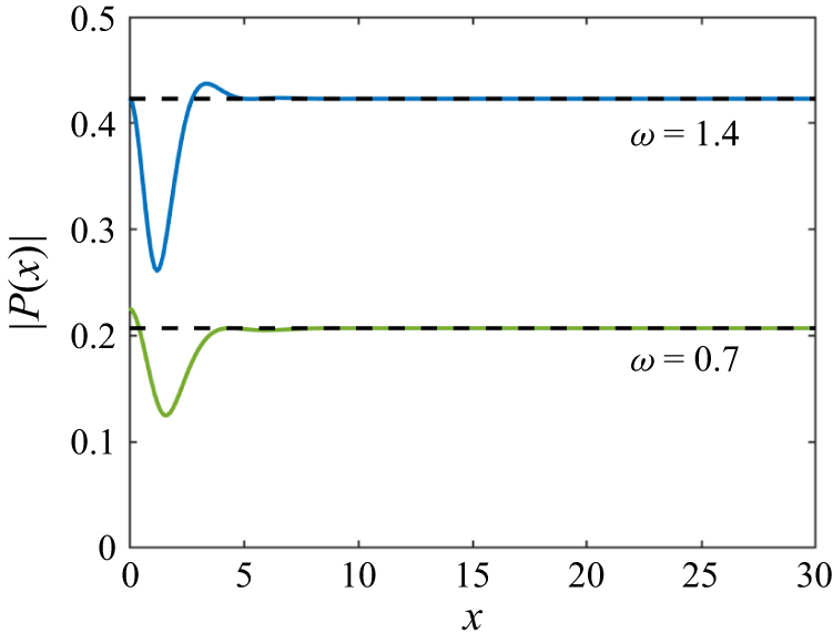
The absolute value of this function is plotted in figure 2 for two values of dimensionless frequency
 $\omega$
and the parameters of the problem listed in § 4.2. The dashed lines in the figure represent the convergence of
 $|P(x)| \to |1/(\kappa _0 Q_0)|$
for large values of
 $x$
. The shear force on the wall (3.15) can now be written as
 \begin{equation} W_{x x x}^{(1)}(0) = \frac {P(\xi )}{P(0)}. \end{equation}
Plot of the series
 $P(x)$
for two values of the dimensionless frequency
 $\omega$
with the dashed line (- - -) depicting the convergence of
 $P(x)$
as
 $x \to \infty$
.

Equations (3.7), (3.12)–(3.14) provide
 \begin{align} W^{(1)}(x) &= \frac {1}{2 \textrm{i} \omega ^{2}} \sum _{n=-2}^{\infty } \frac {1}{\kappa _{n} Q_{n}}\left \{\textrm{e}^{\textrm{i} \kappa _{n}(x+\xi )}+\textrm{e}^{\textrm{i} \kappa _{n}(x-\xi )}- 2 W_{x x x}^{(1)}(0) \textrm{e}^{\textrm{i} \kappa _{n} x}\right \} \quad (x\gt \xi ), \end{align}
 \begin{align} W^{(1)}(x) &= \frac {1}{2 \textrm{i} \omega ^{2}} \sum _{n=-2}^{\infty } \frac {1}{\kappa _{n} Q_{n}}\left \{\textrm{e}^{\textrm{i} \kappa _{n}(x+\xi )}+\textrm{e}^{-\textrm{i} \kappa _{n}(x-\xi )} -2 W_{x x x}^{(1)}(0) \textrm{e}^{\textrm{i} \kappa _{n} x}\right \} \quad (0\lt x\lt \xi ). \end{align}
It is seen that the representations (3.18) and (3.19) of the leading-order deflection in
 $x\gt \xi$
and
 $0\lt x\lt \xi$
are similar. Note that for
 $n \geqslant 1$
, we have
 $\kappa _{n}=i \mu _{n}, \mu _{n}\gt 0$
,
 \begin{align} & \textrm{e}^{\textrm{i} \kappa _{n}(x+\xi )}=-\textrm{e}^{-\mu _{n}(x+\xi )}, \quad \textrm{e}^{\textrm{i} \kappa _{n}(x-\xi )}=\textrm{e}^{-\mu _{n}(x-\xi )} \quad (x\gt \xi ), \end{align}
 \begin{align} & \textrm{e}^{-\textrm{i} \kappa _{n}(x-\xi )}=\textrm{e}^{-\mu _{n}(\xi -x)}, \quad \textrm{e}^{\textrm{i} \kappa _{n} x}=\textrm{e}^{-\mu _{n} x} \quad (0\lt x\lt \xi ). \end{align}
The terms in (3.20) and (3.21) decay exponentially as
 $n \rightarrow \infty$
in the corresponding intervals of
 $x$
. The only value of the
 $x$
coordinate, where the series (3.18) and (3.19) do not converge exponentially, is
 $x=\xi$
, where
 \begin{equation} W^{(1)}(\xi ) = \frac {1}{2 \textrm{i} \omega ^{2}} \sum _{n=-2}^{\infty } \frac {1}{\kappa _{n} Q_{n}}\left \{\textrm{e}^{2{i} \kappa _{n} \xi }+1- 2 W_{x x x}^{(1)}(0) \textrm{e}^{\textrm{i} \kappa _{n} \xi }\right \}. \end{equation}
The series (3.22) converges as
 $O (n^{-9} )$
, which is still quick convergence for numerical evaluations of the corresponding series.
The second derivative of the leading-order deflection at the wall, which is required to estimate the strains there, is
 \begin{align} W_{x x}^{(1)}(0) & =\sum _{n=-2}^{\infty }-\kappa _{n}^{2}\left ( B_{n}+ C_{n}\right ) \end{align}
 \begin{align} & =\frac {P(\xi )P''(0) - P''(\xi )P(0)}{\textrm{i} \omega ^2}. \end{align}
Similarly, the expression for the leading order potential
 $\varphi ^{(1)}(x,y)$
obtained from (3.6), (3.12)–(3.14) is
 \begin{align} \varphi ^{(1)}(x,y) &= \frac {1}{2 \textrm{i} \omega ^{2}} \sum _{n=-2}^{\infty } \frac {f_n(y)}{\kappa _{n} Q_{n}}\left \{\textrm{e}^{\textrm{i} \kappa _{n}(x+\xi )}+\textrm{e}^{\textrm{i} \kappa _{n}(x-\xi )}- 2 W_{x x x}^{(1)}(0) \textrm{e}^{\textrm{i} \kappa _{n} x}\right \} \quad (x\gt \xi ), \end{align}
 \begin{align} \varphi ^{(1)}(x,y) &= \frac {1}{2 \textrm{i} \omega ^{2}} \sum _{n=-2}^{\infty } \frac {f_n(y)}{\kappa _{n} Q_{n}}\left \{\textrm{e}^{\textrm{i} \kappa _{n}(x+\xi )}+\textrm{e}^{-\textrm{i} \kappa _{n}(x-\xi )} -2 W_{x x x}^{(1)}(0) \textrm{e}^{\textrm{i} \kappa _{n} x}\right \} \quad (0\lt x\lt \xi ). \end{align}
A detailed verification that the leading-order solution satisfies all boundary conditions and matching conditions at
 $x=\xi$
is provided in supplementary material S2.
3.2. Double frequency component of the second-order solution
The second-order potential
 $\varphi ^{(2)}(x,y)$
in (2.39) and the deflection
 $W^{(2)}(x)$
are solutions of the following boundary value problem, see (2.40) and (2.42),
 \begin{align} \begin{array}{cl} {\nabla} ^{2} \varphi ^{(2)}=0 \quad \left (-H \leqslant y \leqslant 0, \ \ x\gt 0 \right ), \\[6pt] \displaystyle W^{(2)}=\varphi _{y}^{(2)}-\frac {1}{4}\left (W^{(1)} \varphi _{x}^{(1)}\right )_{x} \quad \left (y=0, \ \ x\gt 0\right ), \\[8pt] \displaystyle W_{x x x x}^{(2)}+\big (1-4 \alpha \omega ^{2}\big ) W^{(2)}=4 \omega ^{2} \varphi ^{(2)}+\frac {\omega ^{2}}{2}\!\left \{\frac {3}{2}\!\left (W^{(1)}\!\right )^{2}+\frac {1}{2}\left (\varphi _{x}^{(1)}\!\right )^{2}\right \} \!\quad\! \left (y=0, \ \ x\gt 0 \right ), \\[10pt] W^{(2)}(0)=W_{x}^{(2)}(0)=0, \\[6pt] \dfrac {\partial \varphi ^{(2)}}{\partial x}=0 \quad \left (x=0, \ \ -H \leqslant y \leqslant 0 \right ), \\[8pt] \dfrac {\partial \varphi ^{(2)}}{\partial y}=0 \quad \left ( y=-H, \ x\gt 0 \right ),\\[-18pt] \end{array}\\[-11pt]\nonumber \end{align}
with the far-field condition that there are no incident waves.
The solution to this problem is more complicated than the solution derived in § 3.1. We shall consider solutions in
 $x\gt \xi$
and
 $0\lt x\lt \xi$
separately.
3.2.1. Solution in
 $x\gt \xi$

Using the expressions for
 $\varphi ^{(1)}$
and
 $W^{(1)}$
from (3.6) and (3.7), respectively, we have the following boundary value problem in the sub domain
 $x\gt \xi :$
 \begin{align} & \varphi ^{(2)}_{xx} + \varphi ^{(2)}_{yy}=0 \quad \quad \left (-H \leqslant y \leqslant 0, \ x\gt \xi \right ),\\[-30pt]\nonumber\end{align}
 \begin{align} W^{(2)}=\varphi _{y}^{(2)}+ \frac {1}{4} \left [\sum _{n=-2}^\infty \sum _{m=-2}^\infty \left (\kappa _{n}+\kappa _{m}\right ) \kappa _{m} \ f_{m}(0) \ A_{n} A_{m} \ \textrm{e}^{\textrm{i}\left (\kappa _{n}+\kappa _{m}\right ) x}\right ] \quad \left (y=0, \ x\gt \xi \right ), \\[-30pt] \nonumber \end{align}
 \begin{align}& W_{x x x x}^{(2)}+\left (1-4 \alpha \omega ^{2}\right ) W^{(2)}=4 \omega ^{2} \varphi ^{(2)} \nonumber \\ & +\frac {\omega ^{2}}{4} \sum _{n=-2}^\infty \sum _{m=-2}^\infty A_{n} A_{m} \ \textrm{e}^{\textrm{i}\left (\kappa _{n}+\kappa _{m}\right ) x} \left (3 -\kappa _{n} \kappa _{m} \ f_{n}(0) f_{m}(0)\right ) \quad \left (y=0, \ x\gt \xi \right ), \\[-30pt] \nonumber \end{align}
 \begin{align} \varphi ^{(2)}_y=0 \quad \quad \left (y=-H, \ x\gt \xi \right ). \\[0pt] \nonumber \end{align}
There are no incoming waves from
 $x \to \infty$
.
The special forms of the forcing terms in (3.29) and (3.30) suggest to search a general solution of the problem (3.28)–(3.31) as
 \begin{equation} \begin{aligned} W^{(2)}(x)&= W_p^{(2+)}(x) + W^+(x), \\ W_p^{(2+)}(x) &= \sum _{n=-2}^\infty \sum _{m=-2}^\infty A_{n} A_{m} \ \textrm{e}^{\textrm{i}\left (\kappa _{n}+\kappa _{m}\right ) x} \boldsymbol{\cdot }E_{n m}, \end{aligned} \end{equation}
and
 \begin{equation} \begin{aligned} \varphi ^{(2)}(x, y)&= \varphi ^{(2+)}_p(x, y) + \varPhi ^+(x, y), \\ \varphi ^{(2+)}_p(x, y) &= \sum _{n=-2}^\infty \sum _{m=-2}^\infty A_{n} A_{m} \ \textrm{e}^{\textrm{i}\left (\kappa _{n}+\kappa _{m}\right ) x} \boldsymbol{\cdot }G_{n m}(y). \end{aligned} \end{equation}
Here,
 $W_p^{(2+)}(x)$
and
 $\varphi ^{(2+)}_p(x, y)$
are particular solutions of the problem, and
 $W^+(x)$
and
 $\varPhi ^+(x, y)$
are general solutions of the problem without forcing terms in (3.29) and (3.30), which are obtained in the same way as in § 3.1.
To find a particular solution of the problem, we need the coefficients
 $E_{n m}$
in (3.32) and the functions
 $G_{n m}(y)$
in (3.33). We notice that the forcing term in (3.30) has a symmetric form. This means that changing
 $n \leftrightarrow m$
does not change this term. The forcing term in (3.29) is not in symmetric form, but it should be the same if we change
 $n \leftrightarrow m$
in it. This observation makes it possible to present the forcing term in (3.29) in the following symmetric form:
 \begin{equation} W^{(2)}(x)=\varphi _{y}^{(2)}+ \frac {1}{8} \left [\sum _{n=-2}^\infty \sum _{m=-2}^\infty \left (\kappa _{n}+\kappa _{m}\right ) \left (\kappa _{n} f_{n}(0) + \kappa _{m} f_{m}(0)\right ) \ A_{n} A_{m} \ \textrm{e}^{\textrm{i}\left (\kappa _{n}+\kappa _{m}\right ) x}\right ]. \end{equation}
The symmetry of the forcing terms suggest that
 $E_{n m} = E_{m n}$
and
 $G_{n m}(y) = G_{m n}(y)$
.
The Laplace equation (3.28), the bottom boundary condition (3.31) and the series in (3.33) provide the boundary value problem for
 $G_{n m}(y)$
,
 \begin{align} G_{n m}^{\prime \prime }(y)-\left (\kappa _{n}+\kappa _{m}\right )^{2} G_{n m}(y) &= 0 \quad (-H \lt y \lt 0), \end{align}
 \begin{align} G_{n m}^{\prime }(-H) &= 0, \end{align}
which has a solution
 \begin{equation} G_{n m}(y)= G_{n m}(0) \ \frac {\cosh \left [\left (\kappa _{n}+\kappa _{m}\right )\left (y+H\right )\right ]}{ \cosh \left [\left (\kappa _{n}+\kappa _{m}\right ) H\right ]}. \end{equation}
In particular,
 \begin{equation} G_{n m}^{\prime }(0)= G_{n m}(0) \ (\kappa _n + \kappa _m) \tanh \left [\left (\kappa _{n}+\kappa _{m}\right ) H\right ]. \end{equation}
The series in (3.32), (3.33), the kinematic boundary condition (3.29) and the relation (3.38) give
 \begin{equation} E_{n m}=G_{n m}(0) \left (\kappa _{n}+\kappa _{m}\right ) \tanh \left [\left (\kappa _{n}+\kappa _{m}\right ) H\right ] +\frac {1}{8}\left (\kappa _{n}+\kappa _{m}\right ) \left (\kappa _{n} f_{n}(0) + \kappa _{m} f_{m}(0)\right ). \end{equation}
Correspondingly, the dynamic condition (3.30) gives
 \begin{equation} \left [\left (\kappa _{n}+\kappa _{m}\right )^4 + 1-4 \alpha \omega ^{2}\right ] E_{n m} =4 \omega ^{2} G_{n m}(0)+\frac {\omega ^{2}}{4} \left (3 -\kappa _{n} \kappa _{m} \ f_{n}(0) f_{m}(0)\right ). \end{equation}
The algebraic system (3.39) and (3.40) confirms that the coefficients
 $E_{n m}$
and
 $G_{n m}(y)$
are symmetric,
 $E_{n m}=E_{m n}$
and
 $G_{n m}(y)=G_{m n}(y)$
. It will be shown later that the coefficients
 $E_{n m}$
and
 $G_{n m}(0)$
increase as
 $n$
and/or
 $m$
tend to infinity. However, the coefficient
 $A_n$
given by (3.12) quickly decay as
 $n \rightarrow \infty$
. It will be shown that the products
 $A_{n} A_{m} E_{n m}$
and
 $A_{n} A_{m} G_{n m}(0)$
in (3.32) and (3.33) respectively decay quickly enough to guarantee convergence of double series in (3.32) and (3.33). Note also that the terms
 $\textrm{e}^{\textrm{i} \kappa _{n} x}$
and
 $\textrm{e}^{\textrm{i} \kappa _{m} x}$
for
 $x\gt \xi$
and
 $n \rightarrow \infty , m \rightarrow \infty$
behave as
 $\textrm{e}^{-\mu _{n} x}$
and
 $\textrm{e}^{-\mu _{m} x}$
, where
 $\mu _{n}\gt 0, \mu _{m}\gt 0$
and
 $\mu _{n}=\mathcal{O}(n)$
as
 $n \rightarrow \infty$
. This implies that the series in (3.32) and (3.33) converge exponentially.
To solve the system (3.39) and (3.40) in a form convenient for calculations of the coefficients
 $E_{n m}$
and
 $G_{n m}(0)$
, the following quantities are introduced:
 \begin{align} R_{n m} &= \left (\kappa _{n}+\kappa _{m}\right ) \tanh \left [\left (\kappa _{n}+\kappa _{m}\right ) H\right ], \end{align}
 \begin{align} S_{n m} &= \frac {\omega ^{2}}{4} \left (3 -\kappa _{n} \kappa _{m} \ f_{n}(0) f_{m}(0)\right ), \end{align}
 \begin{align} N_{n m} &= \frac {\left (\kappa _{n}+\kappa _{m}\right ) \left (\kappa _{n} f_{n}(0) + \kappa _{m} f_{m}(0)\right )}{8}, \end{align}
 \begin{align} V_{n m} &= \left (\kappa _{n}+\kappa _{m}\right )^4 + 1-4 \alpha \omega ^{2}. \end{align}
Then, the solution of the system is
 \begin{align} E_{n m} &= \frac {S_{n m} R_{n m} - 4 \omega ^2 N_{n m}}{R_{n m} V_{n m} - 4 \omega ^2}, \end{align}
 \begin{align} G_{n m}(0) &= \frac {S_{n m} - V_{n m} N_{n m}}{R_{n m} V_{n m} - 4 \omega ^2}. \end{align}
The case
 $R_{n m} V_{n m}=4 \omega ^{2}$
defines the primary resonance of the second-order solution. It can be shown that the denominator
 $R_{n m} V_{n m} - 4 \omega ^2$
is equal to zero at such frequencies
 $\omega$
that
 $\kappa _n,\kappa _m$
are solutions of the dispersion relation (3.2) and the sum
 $\kappa _n + \kappa _m$
is solution of the same equation, but for the double frequency
 $2 \omega$
. At this resonance condition, the (3.39) and (3.40) are linearly dependent and we can take, for example,
 $E_{n m}=R_{n m}+N_{n m}, G_{n m}(0)=1$
as a particular solution, without loss of generality. If the denominator in (3.45) and (3.46) is close to zero, but not equal to zero, then the values of the coefficients
 $E_{n m}$
and
 $G_{n m}(0)$
are large. This signifies a resonant amplification of the double-frequency component of the second-order solution, leading to its dominant contribution to the total deflection and strain. This resonant interaction is the key mechanism responsible for the substantial second-order effects reported in this study.
The coefficients
 $E_{n m}$
and
 $G_{n m}(0)$
can be rewritten in the following computationally efficient form (details in supplementary material S3):
 \begin{align} E_{n m} &= \frac {\kappa _n^5 \kappa _m^5}{(\kappa _n + \kappa _m)^4} \ \widetilde {E}_{n m}, \end{align}
 \begin{align} G_{n m}(0) &= \kappa _n^5 \kappa _m^5 \widetilde {G}_{n m}, \end{align}
where
 $\widetilde {E}_{n m}$
and
 $\widetilde {G}_{n m}$
are bounded for any
 $n$
and
 $m$
.
The particular solution
 $\varphi ^{(2+)}_p(x, 0)$
at
 $y=0$
can now be written in the following form using (3.12) and (3.48),
 \begin{equation} \varphi ^{(2+)}_p(x, 0)= - \sum _{n=-2}^{\infty } \sum _{m=-2}^{\infty } \frac {\kappa _n^4 \kappa _m^4}{4 \omega ^2 Q_n Q_m} \widetilde {A}_{n} \widetilde {A}_{m} \ \widetilde {G}_{n m} \ \textrm{e}^{\textrm{i}\left (\kappa _{n}+\kappa _{m}\right ) (x-\xi )}, \end{equation}
where
 $\widetilde {A}_{n}=1+\textrm{e}^{2 {i} \kappa _{n} \xi }-2 W_{x x x}^{(1)}(0) \: \textrm{e}^{\textrm{i} \kappa _{n} \xi }$
and
 $\widetilde {A}_{n} \rightarrow 1$
exponentially as
 $n \rightarrow \infty$
. The double series in (3.49) can be calculated as a repeated series, see § 4.1,
 \begin{equation} \varphi ^{(2+)}_p(x, 0)= - \frac {1}{4 \omega ^2} \sum _{n=-2}^{\infty } \frac {\kappa _n^4}{Q_n} \ \widetilde {A}_{n} \ \textrm{e}^{\textrm{i} \kappa _{n} (x-\xi )} \ \sum _{m=-2}^{\infty } \frac {\kappa _m^4}{Q_m} \ \widetilde {A}_{m} \ \widetilde {G}_{n m} \ \textrm{e}^{\textrm{i} \kappa _{m} (x-\xi )}. \end{equation}
Correspondingly, (3.32) yields
 \begin{align} W^{(2+)}_p(x)= - \frac {1}{4 \omega ^2} \sum _{n=-2}^{\infty } \frac {\kappa _n^4}{Q_n} \ \widetilde {A}_{n} \ \textrm{e}^{\textrm{i} \kappa _{n} (x-\xi )} \ \sum _{m=-2}^{\infty } \frac {\kappa _{m}^{4}}{Q_{m}\left (\kappa _{n}+\kappa _{m}\right )^{4}} \ \widetilde {E}_{n m} \ \textrm{e}^{\textrm{i} \kappa _{m}(x-\xi )}. \end{align}
It should be noted that writing the double series (3.49) in the repeated form (3.50) offers improved clarity and practical advantages for numerical implementation, allowing independent control over convergence of the inner and outer sums.
The boundary value problem for the functions
 $W^+(x)$
and
 $\varPhi ^+(x,y)$
in (3.32) and (3.33) is formulated as
 \begin{align} {\nabla} ^{2} \varPhi ^+=0 \quad & \left (-H \leqslant y \leqslant 0, \ \ x\gt \xi \right ),\\[-32pt]\nonumber\end{align}
 \begin{align} W^+=\varPhi ^+_{y} \quad & \left ( y=0, \ \ x\gt \xi \right ),\\[-32pt]\nonumber\end{align}
 \begin{align} W^+_{x x x x}+\big (1-4 \alpha \omega ^{2}\big ) W^+=4 \omega ^{2} \varPhi ^+ \quad & \left ( y=0, \ \ x\gt \xi \right ),\\[-32pt]\nonumber\end{align}
 \begin{align} \varPhi ^+_y=0 \quad & \left ( y=-H, \ \ x\gt \xi \right ).\end{align}
There are no incident waves from
 $x = \infty$
and no forcing in (3.52)–(3.55).
The homogeneous problem (3.52)–(3.55), where
 $x\gt \xi$
, is similar to (2.35) and (2.36), but with
 $\omega$
being replaced by
 $2 \omega$
and
 $P_{\textit{ext}}(x) =0$
. The dispersion relation for the problem (3.52)–(3.55) is the relation (3.2) with
 $\omega$
replaced with
 $2 \omega$
. The roots of this dispersion relation with
 $\omega \to 2 \omega$
are different from
 $\kappa _n$
and are denoted as
 $\widehat {\kappa }_n$
. They are calculated independently. Similar to the solution of the leading-order problem in § 3.1, we can write
 \begin{align} \varPhi ^+(x,y) &= \sum _{n=-2}^{\infty } \widehat {A}_{n} \ \textrm{e}^{\textrm{i} \widehat {\kappa }_{n} x} \widehat {f}_{n}(y) \quad \left (-H \leqslant y \leqslant 0, \ \ x\gt \xi \right ), \end{align}
 \begin{align} W^+(x) &= \sum _{n=-2}^{\infty } \widehat {A}_{n} \ \textrm{e}^{\textrm{i} \widehat {\kappa }_{n} x} \quad \quad \quad \quad (x\gt \xi ), \end{align}
see (3.6) and (3.7), with undetermined coefficients
 $\widehat {A}_{n}$
. Here
 $\,\widehat {}\,$
stands for quantities related to the second-order problem with
 $\widehat {A}_{n} \neq A_{n}$
,
 $\widehat {\kappa }_{n} \neq \kappa _{n}$
and
 $\widehat {f}_{n}(y) \neq f_{n}(y)$
,
 $\widehat {\kappa }_{n}$
are the roots of the dispersion relation
 \begin{equation} \big ( \widehat {\kappa }^{4}+1- 4 \alpha \omega ^{2}\big ) \ \widehat {\kappa } \tanh \left (H \widehat {\kappa } \right )= 4 \omega ^{2}, \end{equation}
and the vertical modes
 $\widehat {f}_{n}(y)$
are given by
 \begin{equation} \widehat {f}_{n}(y)=\frac {\cosh \widehat {\kappa }_{n}\left (y+H\right )}{\widehat {\kappa }_{n} \sinh \left (\widehat {\kappa }_{n} H\right )}, \quad n \geqslant -2. \end{equation}
Similar to the modes
 $f_{n}(y)$
, the vertical modes
 $\widehat {f}_{n}(y)$
(3.59) are non-orthogonal in a standard sense, but obey the orthogonality relation
 \begin{equation} \left \langle \widehat {f}_{m}, \widehat {f}_{n}\right \rangle =\delta _{m n} \widehat {Q}_{n}, \quad n,m \geqslant -2, \end{equation}
where the above-mentioned scalar product is defined as
 \begin{align} \left \langle \widehat {F}, \widehat {G}\right \rangle = \int _{-H}^{0} \widehat {F}(y) \widehat {G}(y) \ \textrm{d} y+\frac {1}{4\omega ^{2}} \Big (\widehat {F}^{\prime \prime \prime }(0) \ \widehat {G}^{\prime }(0) + \widehat {F}^{\prime }(0) \ \widehat {G}^{\prime \prime \prime }(0)\Big ) \end{align}
and
 \begin{equation} \widehat {Q}_{n}=\frac {H \widehat {\kappa }_{n}^{2}\left (\widehat {\kappa }_{n}^{4}+1-4\alpha \omega ^{2}\right )^{2}+4\omega ^{2}\left (5 \widehat {\kappa }_{n}^{4}+1-4\alpha \omega ^{2}-4\omega ^{2}H\right )}{32\: \widehat {\kappa }_{n}^{2} \: \omega ^{4}}. \end{equation}
Next, a general solution in the sub-domain
 $0\lt x\lt \xi$
will be determined and matched at
 $x=\xi$
with the solution in the sub-domain
 $x\gt \xi$
to arrive at the second-order solution of the original problem with double frequency.
3.2.2. Solution in
$0\lt x\lt \xi$

The boundary value problem (3.27) in the sub-domain
 $0\lt x\lt \xi$
reads
 \begin{align} \varphi ^{(2)}_{xx} + \varphi ^{(2)}_{yy}=0 \quad \quad (-H \leqslant y \leqslant 0, \ 0\lt x\lt \xi ), \\[-30pt]\nonumber \end{align}
 \begin{align} & W^{(2)}=\varphi _{y}^{(2)} \nonumber \\ & \hspace {0cm} + \frac {1}{4} \!\sum _{n=-2}^{\infty } \!\sum _{m=-2}^{\infty } \Bigg \{ \left (\kappa _{n}+\kappa _{m}\right ) \left [ B_{n} B_{m} \ \textrm{e}^{\textrm{i}\left (\kappa _{n}+\kappa _{m}\right ) x}+ C_{n} C_{m} \ \textrm{e}^{-\textrm{i}\left (\kappa _{n}+\kappa _{m}\right ) x} \right ] (\kappa _{n} f_{n}(0) + \kappa _{m} f_{m}(0)) \nonumber \\ & \hspace {0cm} +\left (\kappa _{n}-\kappa _{m}\right ) \left [ B_{n} C_{m} \ \textrm{e}^{\textrm{i}\left (\kappa _{n}-\kappa _{m}\right ) x} + B_{m} C_{n} \ \textrm{e}^{-\textrm{i}\left (\kappa _{n}-\kappa _{m}\right ) x} \right ] \left (\kappa _{n} f_{n}(0) - \kappa _{m} f_{m}(0)\right ) \Bigg \} \nonumber \\ & \hspace {4cm} \quad (y=0, \ 0\lt x\lt \xi ), \\[-30pt]\nonumber \end{align}
 \begin{align} & W_{x x x x}^{(2)}+\left (1-4 \alpha \omega ^{2}\right ) W^{(2)}=4 \omega ^{2} \varphi ^{(2)} \nonumber \\ & \hspace {0cm} +\frac {\omega ^{2}}{4} \sum _{n=-2}^{\infty } \sum _{m=-2}^{\infty } \Bigg \{ \left (3 -\kappa _{n} \kappa _{m} \ f_{n}(0) f_{m}(0)\right ) \left [ B_{n} B_{m} \ \textrm{e}^{\textrm{i}\left (\kappa _{n}+\kappa _{m}\right ) x} + C_{n} C_{m} \ \textrm{e}^{-\textrm{i}\left (\kappa _{n}+\kappa _{m}\right ) x} \right ] \nonumber \\ & \hspace {0cm} + \left (3 + \kappa _{n} \kappa _{m} \ f_{n}(0) f_{m}(0)\right ) \left [ B_{n} C_{m} \ \textrm{e}^{\textrm{i}\left (\kappa _{n}-\kappa _{m}\right ) x} + B_{m} C_{n} \ \textrm{e}^{-\textrm{i}\left (\kappa _{n}-\kappa _{m}\right ) x} \right ] \Bigg \} \nonumber \\ & \hspace {4cm} \quad (y=0, \ 0\lt x\lt \xi ),\\[-27pt]\nonumber \end{align}
 \begin{align} & W^{(2)}=W_{x}^{(2)}=0 \quad \quad (x=0),\\[-30pt]\nonumber\end{align}
 \begin{align} & \varphi ^{(2)}_x=0 \quad \quad \quad \quad \quad (x=0, \ -H \leqslant y \leqslant 0),\\[-30pt]\nonumber\end{align}
 \begin{align} & \varphi ^{(2)}_y=0 \quad \quad \quad \quad \quad (y=-H, \ 0\lt x\lt \xi ).\end{align}
We seek a general solution in the form
 \begin{align} W^{(2)}(x) &= W^{(2-)}_p(x) + W^-(x), \nonumber \\ W^{(2-)}_p(x) & = \sum _{n=-2}^{\infty } \sum _{m=-2}^{\infty } \Big [B_{n} B_{m} \ \textrm{e}^{\textrm{i}\left (\kappa _{n}+\kappa _{m}\right ) x} \ F_{n m}^{(1)} + C_{n} C_{m} \ \textrm{e}^{-\textrm{i}\left (\kappa _{n}+\kappa _{m}\right ) x} \ F_{n m}^{(2)} \nonumber \\ & \hspace {0cm} + B_{n} C_{m} \ \textrm{e}^{\textrm{i}\left (\kappa _{n}-\kappa _{m}\right ) x} \ F_{n m}^{(3)} +B_{m} C_{n} \ \textrm{e}^{-\textrm{i}\left (\kappa _{n}-\kappa _{m}\right ) x} \ F_{n m}^{(4)} \Big ], \end{align}
and
 \begin{align} \varphi ^{(2)}(x, y) & = \varphi ^{(2-)}_p(x, y) +\varPhi ^-(x, y), \nonumber \\ \varphi ^{(2-)}_p(x, y) &= \sum _{n=-2}^{\infty } \sum _{m=-2}^{\infty } \Big [B_{n} B_{m} \ \textrm{e}^{\textrm{i}\left (\kappa _{n}+\kappa _{m}\right ) x} \ H_{n m}^{(1)}(y) + C_{n} C_{m} \ \textrm{e}^{-\textrm{i}\left (\kappa _{n}+\kappa _{m}\right ) x} \ H_{n m}^{(2)}(y) \nonumber \\ & +B_{n} C_{m} \ \textrm{e}^{\textrm{i}\left (\kappa _{n}-\kappa _{m}\right ) x} \ H_{n m}^{(3)}(y) +B_{m} C_{n} \ \textrm{e}^{-\textrm{i}\left (\kappa _{n}-\kappa _{m}\right ) x} \ H_{n m}^{(4)}(y) \Big ]. \end{align}
Here, the functions
 $W^{(2-)}_p(x)$
and
 $\varphi ^{(2-)}_p(x, y)$
correspond to a particular solution of the problem, while
 $W^-(x)$
and
 $\varPhi ^-(x, y)$
are general solutions of the problem in the sub-domain
 $0\lt x\lt \xi$
without forcing terms in (3.64), (3.65), and with non-homogeneous boundary and edge conditions at
 $x=0$
.
The derivation of the coefficients
 $F_{n m}^{(i)}$
and
 $H_{n m}^{(i)}(y), \,i=1,2,3,4$
follows the same procedure as that outlined in § 3.2.1. The detailed calculations are provided in supplementary material S3. Finally, we have
 \begin{align} W^{(2-)}_p(x) & = \sum _{n=-2}^{\infty } \sum _{m=-2}^{\infty } \Big [B_{n} B_{m} \ \textrm{e}^{\textrm{i}\left (\kappa _{n}+\kappa _{m}\right ) x} + C_{n} C_{m} \ \textrm{e}^{-\textrm{i}\left (\kappa _{n}+\kappa _{m}\right ) x} \Big ] \ E_{n m} \nonumber \\ & + \sum _{n=-2}^{\infty } \sum _{m=-2}^{\infty } \Big [ B_{n} C_{m} \ \textrm{e}^{\textrm{i}\left (\kappa _{n}-\kappa _{m}\right ) x} +B_{m} C_{n} \ \textrm{e}^{-\textrm{i}\left (\kappa _{n}-\kappa _{m}\right ) x} \Big ] \ F_{n m}. \end{align}
The functions
 $W^-(x)$
and
 $\varPhi ^-(x,y)$
appearing in the expressions (3.69) and (3.70), respectively, satisfy the following equations:
 \begin{align} {\nabla} ^{2} \varPhi ^-&=0 \quad \quad (-H \leqslant y \leqslant 0, \ 0\lt x\lt \xi ),\\[-36pt]\nonumber\end{align}
 \begin{align} W^-&=\varPhi ^-_{y} \quad \quad (y=0, \ 0\lt x\lt \xi ),\\[-36pt]\nonumber\end{align}
 \begin{align} W^-_{x x x x}+\left (1-4 \alpha \omega ^{2}\right ) W^-&=4 \omega ^{2} \varPhi ^- \quad \quad (y=0, \ 0\lt x\lt \xi ),\\[-36pt]\nonumber\end{align}
 \begin{align} \dfrac {\partial \varPhi ^-}{\partial y}&=0 \quad \quad (y=-H, \ 0\lt x\lt \xi ),\\[-36pt]\nonumber\end{align}
 \begin{align} \dfrac {\partial \varPhi ^-}{\partial x}(0,y)&= - \sum _{n=-2}^{\infty } \sum _{m=-2}^{\infty } \Bigg \{ \textrm{i}\left (\kappa _{n}+\kappa _{m}\right ) G_{n m}(y) \Big [ B_{n} B_{m} - C_{n} C_{m} \Big ] \nonumber \\ & \quad + \textrm{i} \left (\kappa _{n}-\kappa _{m}\right ) H_{n m}(y) \Big [ B_{n} C_{m} - B_{m} C_{n} \Big ] \Bigg \} \quad (-H \leqslant y \leqslant 0),\\[-36pt]\nonumber\end{align}
 \begin{align} W^-(0) &= - \sum _{n=-2}^{\infty } \sum _{m=-2}^{\infty } E_{n m} \Big [B_{n} B_{m} + C_{n} C_{m} \Big ] + F_{n m} \Big [ B_{n} C_{m} + B_{m} C_{n} \Big ],\\[-36pt]\nonumber\end{align}
 \begin{align} W^{-\prime }(0) &= -\sum _{n=-2}^{\infty } \sum _{m=-2}^{\infty } \Bigg \{ \textrm{i}\left (\kappa _{n}+\kappa _{m}\right ) E_{n m} \Big [ B_{n} B_{m} - C_{n} C_{m} \Big ] \nonumber \\ & \hspace {0cm} + \textrm{i} \left (\kappa _{n}-\kappa _{m}\right ) F_{n m} \Big [ B_{n} C_{m} - B_{m} C_{n} \Big ] \Bigg \}.\end{align}
Following the analysis for the region
 $x\gt \xi$
in § 3.2.1, we notice that the problem (3.72)–(3.78) for
 $0\lt x\lt \xi$
is similar to (2.35) and (2.36) with
 $\omega$
replaced with
 $2 \omega$
and
 $P_{\textit{ext}} =0$
. Additionally, now we have the non-homogeneous boundary condition (3.76) and two non-zero edge conditions (3.77) and (3.78) at
 $x=0$
, unlike the leading order problem in the sub-domain
 $0\lt x\lt \xi$
, where these boundary conditions were homogeneous.
The functions
 $\varPhi ^-(x,y)$
and
 $W^-(x)$
are searched in the region
 $0\lt x\lt \xi$
in the form
 \begin{align} \varPhi ^-(x,y) &= \sum _{n=-2}^{\infty } \widehat {B}_{n} \ \textrm{e}^{\textrm{i} \widehat {\kappa }_{n} x} \widehat {f}_{n}(y) + \widehat {C}_{n} \ \textrm{e}^{-\textrm{i} \widehat {\kappa }_{n} x} \widehat {f}_{n}(y) \quad \left (-H \leqslant y \leqslant 0, \ \ 0\lt x\lt \xi \right ), \end{align}
 \begin{align} W^-(x) &= \sum _{n=-2}^{\infty } \widehat {B}_{n} \ \textrm{e}^{\textrm{i} \widehat {\kappa }_{n} x} + \widehat {C}_{n} \ \textrm{e}^{-\textrm{i} \widehat {\kappa }_{n} x} \quad \quad \quad \quad \quad \quad (0\lt x\lt \xi ). \end{align}
Note that
 $\widehat {B}_{n} \neq B_{n}$
,
 $\widehat {C}_{n} \neq C_{n}$
,
 $\widehat {\kappa }_{n} \neq \kappa _{n}$
and
 $\widehat {f}_{n}(y) \neq f_{n}(y)$
.
The coefficients
 $\widehat {A}_{n},$
 $\widehat {B}_{n}$
and
 $\widehat {C}_{n}$
appearing in (3.56), (3.57), (3.79) and (3.80) are determined using the boundary condition (3.76) at the vertical wall, the edge conditions (3.77), (3.78) and the continuity of the potential together with its horizontal first derivative at
 $x=\xi$
. It is important to note that, unlike in § 3.1, the expressions of these coefficients here are quite complex, which is due to the discontinuity of the particular solution at
 $x=\xi$
. The details are provided in supplementary material S4. Finally, in this way, we obtain the deflection
 $W^{(2)}(x)$
and the velocity potential
 $\varphi ^{(2)}(x,y)$
of the double frequency component of the second-order solution.
3.3. Time-independent component of the second-order solution
The second-order potential
 $\varphi ^{(2)}_0(x,y)$
in (2.39) and the deflection
 $W^{(2)}_0(x)$
are solutions of the following boundary value problem, see (2.41) and (2.43):
 \begin{align} {\nabla} ^{2} \varphi ^{(2)}_0=0 \quad & \left (-H \leqslant y \leqslant 0, \ x\gt 0 \right ),\\[-30pt]\nonumber\end{align}
 \begin{align} \displaystyle \frac {\partial \varphi _{0}^{(2)}}{\partial y}=-\frac {1}{4}\left (W^{(1)} \bar {\varphi }_{x}^{(1)}\right )_{x} \quad & \left (y=0, \ x\gt 0\right ),\\[-30pt]\nonumber\end{align}
 \begin{align} \displaystyle \frac {\partial ^{4} W_{0}^{(2)}}{\partial x^{4}}+W_{0}^{(2)}=\frac {\omega ^{2}}{4}\left \{\left |W^{(1)}\right |^{2}-\left |\varphi _{x}^{(1)}\right |^{2}\right \} \quad & \left (y=0, \ x\gt 0\right ),\\[-30pt]\nonumber\end{align}
 \begin{align} W_0^{(2)}=W_{0x}^{(2)}=0 \quad & \left ( x=0\right ),\\[-30pt]\nonumber\end{align}
 \begin{align} \dfrac {\partial \varphi _0^{(2)}}{\partial x}=0 \quad & \left (x=0, \ -H \leqslant y \leqslant 0\right ),\\[-30pt]\nonumber\end{align}
 \begin{align} \dfrac {\partial \varphi _0^{(2)}}{\partial y}=0 \quad & \left (y=-H, \ x\gt 0\right ).\end{align}
The solution to this problem is obtained in a manner similar to that used for the double frequency component of the second-order solution in § 3.2. The solution of the problem should contain no incident waves as
 $x \to \infty$
. Note that the problem (3.81)–(3.86) is decoupled, which means that the plate deflection and the velocity potential can be solved for independently rather than simultaneously as was done in § 3.2. The deflection
 $W_0^{(2)}(x)$
is obtained as the solution of the problem (3.83)–(3.84), which satisfies the far-field condition. Then, the potential
 $\varphi ^{(2)}_0(x,y)$
is determined as the solution of the problem (3.81), (3.82), (3.85) and (3.86). As before, we start with the general solutions in regions
 $x\gt \xi$
and
 $0\lt x\lt \xi$
separately.
The forcing term on the right-hand side of the dynamic condition (3.83) can be expressed using the leading order solutions
 $ W^{(1)}(x)$
and
 $ \varphi ^{(1)}(x, y)$
given by (3.7) and (3.6) as
 \begin{equation} F(x) = \frac {\omega ^2}{4} \sum _{n=-2}^{\infty } \sum _{m=-2}^{\infty } \left ( 1 - \kappa _n \bar {\kappa }_m f_n(0) \bar {f}_m(0) \right ) A_n \bar {A}_m \textrm{e}^{\textrm{i} (\kappa _n - \bar {\kappa }_m) x} \quad ( x \gt \xi ) \end{equation}
and
 \begin{align} F(x) &= \frac {\omega ^{2}}{4} \sum _{n=-2}^{\infty } \sum _{m=-2}^{\infty } \Bigg \{ \left (1 -\kappa _{n} \bar {\kappa }_{m} \ f_{n}(0) \bar {f}_{m}(0)\right ) \left [ B_{n} \bar {B}_{m} \ \textrm{e}^{\textrm{i}\left (\kappa _{n}-\bar {\kappa }_{m} \right ) x} + C_{n} \bar {C}_{m} \ \textrm{e}^{-\textrm{i}\left (\kappa _{n}-\bar {\kappa }_{m}\right ) x} \right ] \nonumber \\ & \hspace {0cm} + \left (1 + \kappa _{n} \bar {\kappa }_{m} \ f_{n}(0) \bar {f}_{m}(0)\right ) \left [ B_{n} \bar {C}_{m} \ \textrm{e}^{\textrm{i}\left (\kappa _{n}+\bar {\kappa }_{m}\right ) x} + \bar {B}_{m} C_{n} \ \textrm{e}^{-\textrm{i}\left (\kappa _{n}+\bar {\kappa }_{m}\right ) x} \right ] \Bigg \}, \end{align}
where
 $ 0 \lt x \lt \xi$
.
The form of the forcing term (3.87), suggests the following form of the general solution
 $W_0^{(2)}(x)$
in the sub-domain
 $ x \gt \xi$
:
 \begin{align} W_0^{(2)}(x) &= W_{0p}^{(2+)}(x) + W_{0g}^+(x), \nonumber \\ W_{0p}^{(2+)}(x) &= \sum _{n=-2}^{\infty } \sum _{m=-2}^{\infty } A_n \bar {A}_m \textrm{e}^{\textrm{i} (\kappa _n - \bar {\kappa }_m) x} \ E_{0nm}, \end{align}
where
 $W_{0p}^{(2+)}(x)$
is the particular solution and
 $W_{0g}^{+}(x)$
is the general solution of the problem in the sub-domain
 $x\gt \xi$
without the forcing term in (3.83).
Substituting the expression (3.89) for the particular solution
 $W_{0p}^{(2+)}(x)$
and the forcing term (3.87) in (3.83), and then comparing both sides, we find
 \begin{equation} E_{0nm} = \frac {\omega ^2 \left [1 - \kappa _n \bar {\kappa }_m f_n(0) \bar {f}_m(0) \right ] }{4 \left (1 + (\kappa _n - \bar {\kappa }_m)^4\right )}. \end{equation}
The general solution
 $W_{0g}^+(x)$
satisfies (3.83) with zero right-hand side. A general solution of this fourth-order linear homogeneous ordinary differential equation, which satisfies the far-field condition, reads
 \begin{equation} W_{0g}^+(x) = \mathcal{A}_1 \ \textrm{e}^{(-1+{i}) \mu x} + \mathcal{A}_2 \ \textrm{e}^{(-1-{i}) \mu x} \quad (x\gt \xi ), \end{equation}
where
 $\mu = 1/\sqrt {2}$
, and
 $\mathcal{A}_1,$
 $\mathcal{A}_2$
are unknown coefficients to be determined.
Similarly, analysing the form of the forcing term from (3.88), we seek the general solution for
 $W_0^{(2)}(x)$
in the sub-domain
 $ 0\lt x \lt \xi$
in the form
 \begin{align} W_0^{(2)}(x) &= W^{(2-)}_{0p}(x) + W_{0g}^-(x), \nonumber \\ W^{(2-)}_{0p}(x) & = \sum _{n=-2}^{\infty } \sum _{m=-2}^{\infty } \Big [B_{n} \bar {B}_{m} \ \textrm{e}^{\textrm{i}\left (\kappa _{n}-\bar {\kappa }_{m}\right ) x} \ F_{0n m}^{(1)} + C_{n} \bar {C}_{m} \ \textrm{e}^{-\textrm{i}\left (\kappa _{n}-\bar {\kappa }_{m}\right ) x} \ F_{0n m}^{(2)} \nonumber \\ & + B_{n} \bar {C}_{m} \ \textrm{e}^{\textrm{i}\left (\kappa _{n}+\bar {\kappa }_{m}\right ) x} \ F_{0n m}^{(3)} +\bar {B}_{m} C_{n} \ \textrm{e}^{-\textrm{i}\left (\kappa _{n}+\bar {\kappa }_{m}\right ) x} \ F_{0n m}^{(4)} \Big ]. \end{align}
Here,
 $W_{0p}^{(2-)}(x)$
is the particular solution and
 $W_{0g}^{-}(x)$
is the general solution of the problem in the sub-domain
 $0\lt x\lt \xi$
without the forcing term in (3.83).
Using the particular solution
 $W^{(2-)}_{0p}(x)$
from (3.92) and the forcing term (3.88) in (3.83), we obtain
 \begin{align} F_{0n m}^{(1)} = F_{0n m}^{(2)} &= E_{0nm}, \end{align}
 \begin{align} F_{0n m}^{(3)} = F_{0n m}^{(4)} &= F_{0nm} = \frac {\omega ^2 \left [1 + \kappa _n \bar {\kappa }_m f_n(0) \bar {f}_m(0) \right ] }{4 \left (1 + (\kappa _n + \bar {\kappa }_m)^4\right )}. \end{align}
Note that the expression on the right-hand side of (3.94) is the same as the expression of
 $E_{0nm}$
in (3.90), but with
 $\bar {\kappa }_m$
replaced with
 $-\bar {\kappa }_m$
.
The function
 $W_{0g}^-(x)$
is a general solution of (3.83) with zero right-hand side,
 \begin{align} W_{0g}^-(x) = \mathcal{B}_1 \ \textrm{e}^{(1+{i}) \mu x} + \mathcal{B}_2 \ \textrm{e}^{(1-{i}) \mu x} + \mathcal{B}_3 \ \textrm{e}^{(-1+{i}) \mu x} + \mathcal{B}_4 \ \textrm{e}^{(-1-{i}) \mu x} \quad (0\lt x\lt \xi ), \end{align}
where
 $\mathcal{B}_1, \mathcal{B}_2, \mathcal{B}_3$
and
 $\mathcal{B}_4$
are the unknown coefficients to be determined. The derivation of these coefficients along with the coefficients
 $\mathcal{A}_1, \mathcal{A}_2$
appearing in (3.91) is provided in supplementary material S5. This yields the deflection
 $W_{0}^{(2)}(x)$
of the time-independent component of the second-order solution.
4. Results and discussion
4.1. Summation of double series with symmetric elements
The double series such as (3.49)–(3.51), as well as many others, in § 3 can be written in the form
 \begin{equation} \mathcal{S} = \sum _{n=-2}^{\infty } \sum _{m=-2}^{\infty } A_{n m}, \end{equation}
where
 $A_{n m} = A_{m n}$
for any
 $n, m \geqslant -2$
. We have
 \begin{align} \mathcal{S} = \sum _{n=-2}^{\infty } A_{n n} + \sum _{n=-1}^{\infty } \sum _{m=-2}^{n-1} A_{n m} + \sum _{m=-1}^{\infty } \sum _{n=-2}^{m-1} A_{n m} = 2 \sum _{n=-1}^{\infty } \sum _{m=-2}^{n-1} A_{n m} + \sum _{n=-2}^{\infty } A_{n n}. \end{align}
For example, the formula (3.51) for
 $x\gt \xi$
would read as
 \begin{align} W^{(2+)}_p(x) &= - \frac {1}{4 \omega ^2} \sum _{n=-2}^{\infty } \frac {\kappa _n^8}{(2 \kappa _n)^4 Q_n^2} \ \tilde {E}_{n n} \ \textrm{e}^{2 {i} \kappa _{n} (x-\xi )} \nonumber \\ & \quad - \frac {1}{2 \omega ^2} \sum _{n=-1}^{\infty } \frac {\kappa _n^4}{Q_n} \textrm{e}^{\textrm{i} \kappa _{n} (x-\xi )} \sum _{m=-2}^{n-1} \frac {\kappa _{m}^{4}}{Q_{m}\left (\kappa _{n}+\kappa _{m}\right )^{4}} \ \tilde {E}_{n m} \ \textrm{e}^{\textrm{i} \kappa _{m}(x-\xi )}. \end{align}
Equation (4.2) helps to accelerate convergence of double series with symmetric elements.
4.2. Convergence of the numerical results
The numerical results corresponding to the hydroelastic vibrations of an ice plate fixed to a wall and subjected to an oscillating point pressure at
 $x=\xi$
are obtained and investigated for ice density
 $\rho _i = 917 \,\textrm{kg m}^{-3}$
, Young’s modulus
 $E = 4.2 \times 10^9 \,\textrm{N m}^{-2}$
, Poisson’s ratio
 $\nu = 0.33$
and ice thickness
 $h_i = 1.5 \,\textrm{m}$
(Squire et al. Reference Squire, Robinson, Langhorne and Haskell1988). Thus, the mass of the ice plate per unit area is
 $M = 1375.5 \,\textrm{kg m}^{-2}$
and the flexural rigidity is
 $D = 1.32\times 10^9\,\textrm{N m}$
. Further, the water density is
 $\rho = 1026 \,\textrm{kg m}^{-3}$
and the physical water depth is
 $H^{\prime } = 15 \,\textrm{m}$
. Hence, the characteristic length of this ice plate is
 $L = 19.05 \,\textrm{m}$
and, correspondingly,
 $\alpha = M/(\rho L) = 0.0704$
. Similar characteristics of ice have been used in several earlier studies, see for example Brocklehurst et al. (Reference Brocklehurst, Korobkin and Părău2010) and Wu et al. (Reference Wu, Khabakhpasheva, Ni and Korobkin2023a
). The water depth is comparable with the characteristic length
 $L$
, which implies that the finite depth matters in our analysis. The frequency and position of the external point pressure will vary in the following calculations.
We obtain the roots
 $\kappa _n$
of the dispersion relation (3.2) using the Wolfram Mathematica software. To check the correctness of the numerical values of these roots, and decide upon a truncation number
 $N$
for the series in (3.6) and (3.7), we calculate the following series ((47) and (88) of Korobkin et al. Reference Korobkin, Malenica and Khabakhpasheva2019):
 \begin{align} l_0 (\omega ) = \sum _{n=-2}^{\infty } \frac {1}{Q_n}, \quad l_1(\omega ) - \omega ^2 = \sum _{n=-2}^{\infty } \frac {\kappa _n^2}{Q_n} - \omega ^2, \quad l_2(\omega ) = \sum _{n=-2}^{\infty } \frac {\kappa _n^4}{Q_n}, \end{align}
which must all be equal to zero for any dimensionless frequency
 $\omega$
.
After performing the numerical calculations for higher values of
 $\omega$
(up to 100), it was observed that the series
 $l_j(\omega ) \,(j=0,1,2)$
keep growing quadratically and their values remain no more close to zero. It is only within the interval
 $(0,3.77)$
that the accuracy of the series
 $l_j$
is in the range
 $10^{-9} {-} 10^{-20}$
, see figures 3 and 4. The decreasing accuracy with increasing
 $\omega$
can be attributed to numerical sensitivity. At high frequencies, the large and oscillatory nature of the wavenumbers
 $\kappa _n$
not only complicates root-finding, but also leads to catastrophic cancellation in the calculation of
 $Q_n$
, where the subtraction of large terms significantly amplifies round-off errors. Similar behaviour of the series was reported by Korobkin et al. (Reference Korobkin, Malenica and Khabakhpasheva2019), where the roots
 $\kappa _n$
were determined using another algorithm. Thus, for all the results hereafter, the dimensionless frequency
 $\omega$
is considered only in the interval
 $(0,3.77)$
, which is for long waves. For a characteristic length
 $L=19.05 \,\textrm{m}$
, this corresponds to a dimensional angular frequency
 $\omega ^\prime$
in the range
 $(0,2.70) \, \textrm{rad s}^{-1}$
, covering long flexural-gravity waves with wavelengths greater than approximately 70 m
 $(\kappa _0^\prime = \kappa _0/L = 1.7431/L)$
. All series in our calculations are truncated at 200 imaginary roots of the dispersion relation (3.2).
Convergence of series
 $l_2$
with the number of imaginary roots of the dispersion relation (3.2) for
 $\omega = 2$
.

The series
 $l_0$
,
 $l_1 - \omega ^2$
and
 $l_2$
against dimensionless frequency
 $\omega$
.

4.3. Limiting cases
4.3.1. Static deflection and the small-frequency limit
In the static regime
 $(\omega \to 0)$
, the fluid is at rest and the velocity potential vanishes,
 $\phi = 0$
. In our original formulation, the static problem reduces to the plate (2.3), where
 $\phi = 0$
, subject to the boundary conditions (2.4) and the far-field condition
 $w \to 0$
as
 $x \to \infty$
. This solution would be valid for arbitrary values of
 $\varepsilon$
. It should be noted that this is a nonlinear problem, which implies that correction to the linear solution is of order
 $\mathcal{O} (\varepsilon ^2 )$
and is due to the nonlinearity of the plate equation only. This nonlinear boundary value problem can be solved numerically. We limit ourselves to the case of small
 $\varepsilon$
.
In the leading order approximation as
 $\varepsilon \to 0,$
the static linear solution can be obtained analytically. Since there is no fluid motion, the right-hand side of (2.17) becomes zero and the leading-order problem reduces to the static fourth-order ordinary differential equation with a point load, whose solution is given by
 \begin{align} W^{(1)}_{\textit{static}}(x) = \begin{cases} \mathcal{C}_1 \ \textrm{e}^{(-1+\textrm{i}) \mu x} + \mathcal{C}_2 \ \textrm{e}^{(-1-\textrm{i}) \mu x} \quad (x\gt \xi ), \\ \mathcal{D}_1 \ \textrm{e}^{(1+\textrm{i}) \mu x} + \mathcal{D}_2 \ \textrm{e}^{(1-\textrm{i}) \mu x} + \mathcal{D}_3 \ \textrm{e}^{(-1+\textrm{i}) \mu x} + \mathcal{D}_4 \ \textrm{e}^{(-1-\textrm{i}) \mu x} \quad (0\lt x\lt \xi ), \end{cases} \end{align}
where
 $\mu = 1/\sqrt {2}$
, and the unknown coefficients
 $\mathcal{C}_1,$
 $\mathcal{C}_2,$
 $\mathcal{D}_1, \mathcal{D}_2, \mathcal{D}_3$
and
 $\mathcal{D}_4$
are determined using the edge conditions (2.18) at the wall, and the matching conditions (3.8) and (3.9) at
 $x=\xi$
.
The second-order problem (2.23)–(2.30) in the static case gives
 $w^{(2)} = 0$
. This is because in the static regime, all time-dependent terms vanish and the fluid potential is zero, reducing (2.25) to a homogeneous equation with homogeneous boundary conditions, see (2.26) and (2.30). Thus, within the second-order approximation, the static deflection is given by
 \begin{equation} w_{\textit{static}}(x) = {\textrm{Re}}\,\{W^{(1)}_{\textit{static}}(x)\} + \mathcal{O}\big (\varepsilon ^2\big ). \end{equation}
To validate our dynamic formulation, we compute the full second-order unsteady solution, derived in § 3, for a small frequency
 $\omega =0.01$
and compare it with the static solution (4.5). In this quasi-static limit, the inertial effects in both the fluid and the ice plate are expected to be negligible. Therefore, no propagating waves are present and the dynamic solution should converge to the static displacement profile. This is confirmed in figure 5, where the second-order dynamic solution for
 $\omega =0.01$
, shown by the solid black curve, matches closely the static solution (4.6) shown by the blue circles.
Comparison of the static deflection profile (4.6) with the unsteady second-order solution for
 $\omega =0.01$
.

4.3.2. Oscillating point pressure at large distance from the wall
Within the leading-order approximation, the wave is generated by an oscillating point pressure applied far from the wall
 $(\xi \gg 1)$
, and propagating towards it can be regarded as an incident wave with frequency
 $\omega$
and dimensionless wavenumber
 $\kappa _0$
. The amplitude of this wave depends on the strength of the external pressure, but is independent of the presence of the wall. For the point pressure given in (2.50), the wave amplitude is equal to
 $|C_0|= 1/(2 \omega ^2 \kappa _0 Q_0)$
, see (3.7) and (3.14). Therefore, our leading-order results for large
 $\xi$
can be directly compared with those of Brocklehurst et al. (Reference Brocklehurst, Korobkin and Părău2010), who studied ice deflection near the wall due to an incident wave. All physical parameters in our calculations, see § 4.2, match those of Brocklehurst et al. (Reference Brocklehurst, Korobkin and Părău2010), except for the water depth and ice thickness, which were
 $H^\prime =350 \,\textrm{m}$
and
 $h_i = 1.6 \,\textrm{m}$
, respectively, in their study. Consequently, this requires updating
 $L = 19.8942 \,\textrm{m}$
and
 $\alpha = 0.0719$
.
We choose
 $\omega = 0.5295$
for the comparison and set
 $\xi =500$
. This frequency
 $\omega$
was selected so as to fit the characteristics of the incident wave used by Brocklehurst et al. (Reference Brocklehurst, Korobkin and Părău2010). Note that Brocklehurst et al. (Reference Brocklehurst, Korobkin and Părău2010) used the water depth as the characteristic length scale, so the dimensionless distance from the wall in their notation was
 $x^{*} = x^\prime /H^\prime$
. To enable a direct comparison, we rescale our results using the same scales. The ice deflection near the wall,
 $0\lt x^*\lt 3$
, is presented in figure 6, where the blue solid line represents our solution and the red dots correspond to data extracted from figure 9(a) of Brocklehurst et al. (Reference Brocklehurst, Korobkin and Părău2010). The comparison demonstrates good agreement between the two solutions.
While the presented framework can be extended to wave scattering problems, this study intentionally focuses on the foundational case of a localised force to systematically isolate and understand the key nonlinear mechanisms such as resonant second-harmonic generation and strain localisation without the added complexity of a full wave scattering problem. While the framework in this subsection demonstrates its capability to model an incident wave field, we chose not to pursue the second-order response for that specific case in this work to maintain a sharp focus on the novel physics of the forced response near a boundary.
Comparison of ice plate deflection near the vertical wall
 $(x=0)$
for waves generated by a distant oscillating pressure
 $(\xi \gg 1)$
and for the incoming wave case studied by Brocklehurst et al. (Reference Brocklehurst, Korobkin and Părău2010).

4.4. Comparison of leading order and second-order strains
The relative elongations (or contractions) of the filaments (or fibres) of an elastic plate are referred to as strains. The elastic strains are maximal on the upper and lower surfaces of the ice plate. In dimensionless variables, they are given by
 \begin{equation} \epsilon (x, t) = \mp \epsilon _{\textit{sc}} \ \frac {\partial ^2 w}{\partial x^2}, \end{equation}
where
 $\epsilon _{\textit{sc}} = (h_i \varepsilon )/(2 L)$
is the strain scale. The negative sign applies to the upper surface of the plate, while the positive sign corresponds to the lower surface. Tensile strain is indicated by a positive value, whereas compressive strain is represented by a negative value. The yield strain for ice
 $\epsilon _Y$
is estimated as
 $8 \times 10^{-5}$
, see Brocklehurst et al. (Reference Brocklehurst, Korobkin and Părău2010) and Korobkin & Khabakhpasheva (Reference Korobkin and Khabakhpasheva2025) for discussions on this value. We assume that the elastic strains in a continuous ice caused by an external load cannot exceed the yield strain value. We use this value as a reference threshold to identify regions where the induced elastic strain is critically high. It is important to note that this value applies to the failure of a free-floating ice plate. The fracture process at the clamped wall is more complex, likely involving localised crushing, spalling or a different failure mode due to the extreme stress concentration and constraint. Therefore, while strains exceeding this yield value in the interior strongly indicate a high risk of crack initiation, the actual failure mechanism at the wall boundary itself may differ and require a separate, more localised analysis (Zou, Xiao & Jordaan Reference Zou, Xiao and Jordaan1996).
Using the asymptotic expansion (2.13) for the ice deflection
 $w(x,t)$
and the expressions (2.33), (2.38) for the leading order deflection
 $w^{(1)}(x,t)$
and the second-order deflection
 $w^{(2)}(x,t)$
, respectively, we obtain the first-order strain
 $\epsilon ^{(1)}(x,t)$
as
 \begin{equation} \frac {\epsilon ^{(1)}}{\epsilon _{\textit{sc}}} =\mp \textrm{Re}\, \left \{ W_{xx}^{(1)}(x) \ \textrm{e}^{-\textrm{i} \omega t}\right \} \end{equation}
and the full second-order strain
 $\epsilon ^{(2)}(x,t)$
as
 \begin{align} \frac {\epsilon ^{(2)}}{\epsilon _{\textit{sc}}} = \mp {Re}\left \{ W_{xx}^{(1)}(x) \textrm{e}^{-\textrm{i} \omega t} + \varepsilon \ W_{xx}^{(2)}(x) \ \textrm{e}^{-2 {i} \omega t} + \varepsilon \ W_{0xx}^{(2)}(x)\right \}. \end{align}
Both strains
 $\epsilon ^{(1)}(x,t)$
, which is predicted by the linear theory, and
 $\epsilon ^{(2)}(x,t)$
, which is the second-order strain determined in the present study, are periodic in time with the period
 $2\pi /\omega$
. In the following, we focus on the maximum in time amplitudes:
 \begin{equation} \epsilon _m^{(1)}(x)= \max _{0 \lt t \lt \frac {2 \pi }{\omega }} |\epsilon ^{(1)}(x,t)| = \epsilon _{\textit{sc}} \ |W^{(1)}_{xx} (x)|, \quad \epsilon _m^{(2)}(x)=\max _{0\lt t \lt \frac {2 \pi }{\omega }} |\epsilon ^{(2)}(x,t)|. \end{equation}
The linear strain amplitude
 $\epsilon _m^{(1)}(x)$
depends on the scale
 $\epsilon _{\textit{sc}}$
, which is proportional to the strength of the external load through the small parameter
 $\varepsilon$
, and the function
 $W^{(1)}(x)$
, which depends on the structural parameter
 $\alpha$
, the dimensionless frequency
 $\omega$
, the dimensionless distance of the application of the load
 $\xi$
from the wall and the dimensionless water depth
 $H$
. Correspondingly, the inequality
 $\epsilon _m^{(1)}(x)\lt \epsilon _Y$
can be treated as a restriction in terms of the parameter
 $\varepsilon$
and finally in terms of the strength of the external point load.
To contextualise the magnitude of the forcing, we define a critical value
 $\varepsilon _*$
that estimates when the linear strain would reach the yield threshold. This provides a reference scale to ensure our weakly nonlinear analysis remains in a physically plausible regime where the ice would not have already fractured according to a linear model. Thus, acceptable values of
 $\varepsilon$
lie in the range
 $0\lt \varepsilon \lt \varepsilon _*$
, where
 \begin{equation} \varepsilon _* = \frac {2 L}{h_i} \: \frac {\epsilon _Y}{\max _{x\geqslant 0} | W_{xx}^{(1)}(x)|}. \end{equation}
We restrict our analysis to
 $0\lt \varepsilon \lt \varepsilon _*$
, ensuring that the linear component of the strain does not surpass the yield strain
 $\epsilon _Y$
. This does not imply the plate model is invalid up to this point; rather, it is a conservative criterion to maintain the relevance of our elastic model before the onset of pervasive plastic deformation or fracture.
Magnitude of
 $W^{(1)}_{xx}(x)$
in the ice plate as a function of
 $x$
for (a) varying values of
 $\xi$
and fixed dimensionless frequency
 $\omega =1.4$
and (b) varying values of
 $\omega$
for fixed
 $\xi = 10$
.

The function
 $|W^{(1)}_{xx}(x)|$
is shown in figure 7 for different
 $\xi$
and the frequency
 $\omega$
. Other parameter values are listed in § 4.2. The figure reveals how the load position
 $\xi$
and frequency
 $\omega$
govern the failure risk. The key finding is a fundamental shift in the location of maximum strain, which dictates where the ice is most likely to fracture. For low frequencies (
 $\omega \lt 0.5$
) and loads positioned away from the wall (
 $\xi \gt 2$
), the maximum strain occurs not at the wall, but directly beneath the load itself (see figure 7
b). Physically, the ice responds quasi-statically, bending locally under the oscillating load. As the frequency increases or the load moves closer to the wall, the behaviour of the system changes. Wave reflection from the rigid boundary becomes dominant, creating a standing wave pattern that pins the maximum strain at the clamped edge (
 $x=0$
), as seen in figure 7(a). The wall, not the load, becomes the critical point of failure.
To illustrate the physical implications, consider a point load
 $190.5\,\textrm{m}$
from the wall (
 $\xi =10$
) oscillating at
 $\omega ^\prime = 0.6\,\textrm{rad s}^{-1}$
(
 $\omega =0.84$
). Our analysis gives
 $\varepsilon _* \approx 0.0036$
, corresponding to a total load magnitude of approximately
 $13.15 \times 10^3 \, \textrm{N m}^{-1}$
, which provides a conservative threshold for critically high elastic strains in the ice plate. This threshold serves as a practical reference for assessing strain localisation under oscillatory loading, rather than a prediction of fracture at the wall. Table 1 summarises this for the parameters in figure 7. A practical problem addressed in this paper concerns engineering activities on floating ice. These include the use of vibrators placed on the ice to investigate ice properties and bottom topography, to detect subsurface flows and moving objects beneath the ice, and to image subsurface geological structures, particularly in the context of oil and gas exploration (Holdsworth & Glynn Reference Holdsworth and Glynn1978; Eisen et al. Reference Eisen, Hofstede, Diez, Kristoffersen, Lambrecht, Mayer, Blenkner and Hilmarsson2015).
Maximum values of the linear strain
 $|W^{(1)}_{xx}(x)|$
and corresponding critical strain amplitudes
 $\varepsilon _*$
for various parameter combinations. Results are extracted from figure 7.

The maximum value
 $\varepsilon _*$
of the small parameter
 $\varepsilon$
as a function of frequency
 $\omega$
and load location
 $\xi$
: (a) full parameter range and (b) magnified view highlighting cases where the load is applied very close to the wall.

To further understand the dependence of ice plate strain response on the frequency and position of the point load, we compute
 $\varepsilon _*$
using the formula (4.11) over a range of non-dimensional frequencies
 $\omega \in (0,3.5]$
and loading locations
 $\xi \in (0,10]$
, see figure 8(a). We observe a minimum values of strains for
 $\xi \gt 3$
and
 $0.5 \lt \omega \lt 3.5$
, and maximum values of strains for small
 $\xi$
. The magnified view in figure 8(b) focuses on cases where the load is applied very close to the wall. To contextualise these values in a physical scenario, we relate the parameter
 $\varepsilon _*$
to a physical load via
 $F_{phys} = \varepsilon _* \rho g L^2$
N m−1. For our parameters (
 $\rho =1026 \,\textrm{kg m}^{-3}$
,
 $L=19.05$
m), the range
 $\varepsilon _* = 0.004-0.022$
investigated corresponds to physical loads of
 $14.6$
kN m−1 to
 $80.4$
kN m−1. Distributed over a characteristic width, this represents the load of a snowmobile (over 0.5 m) up to light aircraft or industrial equipment (over 3 m), confirming the analysis addresses realistic forcing. The figures show that
 $\varepsilon _*$
is more sensitive to the distance of the load from the wall than to the frequency of the load. Note that
 $\xi =0.2$
corresponds to
 $3.81 \,\textrm{m}$
in the dimensional variables, which is small compared with the water depth of
 $15\,\textrm{m}$
in our calculations. The locations,
 $x_{{max}}(\omega ,\xi )$
, where the maximum strains are achieved, are shown in figure 9. Only for frequencies smaller than 0.5 and dimensionless distances
 $\xi \gt 2$
, the maximum strain is achieved not at the wall. For the range
 $\omega \lt 0.5$
and
 $\xi \gt 2$
, the position
 $x_{{max}}$
of the maximum strain tends to coincide with the load position
 $\xi$
. Overall, these findings highlight the strong influence of both the loading frequency and position on the strain distribution. They provide valuable guidance for the design and safe operation of floating structures and point-load systems acting on ice plates.
The
 $x$
-coordinate of the point on the ice plate,
 $x_{{max}}$
, where the maximum of
 $|W^{(1)}_{xx}(x)|$
is achieved.

Strain components for
 $\xi = 0.2$
showing (a,b) magnitude of the leading order scaled strain
 $\epsilon ^{(1)}_m(x)/\epsilon _Y$
and (c,d) the difference between leading and second-order strains scaled by
 $\varepsilon _*$
,
 $(\epsilon _m^{(2)}(x) - \epsilon _m^{(1)}(x) )/\epsilon _Y/\varepsilon _*$
, both as functions of the distance
 $x$
from the wall. Results are shown for (a, c)
 $\omega = 0.0056$
,
 $\varepsilon _* = 0.0117$
and (b,d)
 $\omega = 2.8$
,
 $\varepsilon _* = 0.0132$
.

Strain components for
 $\xi = 5$
showing (a,b) magnitude of the leading order scaled strain
 $\epsilon ^{(1)}_m(x)/\epsilon _Y$
and (c,d) the difference between leading and second-order strains scaled by
 $\varepsilon _*$
,
 $(\epsilon _m^{(2)}(x) - \epsilon _m^{(1)}(x) )/\epsilon _Y/\varepsilon _*$
, both as functions of the distance
 $x$
from the wall. Results are shown for (a, c)
 $\omega = 0.0056$
,
 $\varepsilon _* = 0.00575$
and (b,d)
 $\omega = 2.8$
,
 $\varepsilon _* = 0.00522$
.

Strain components for
 $\xi = 10$
showing (a,b) magnitude of the leading order scaled strain
 $\epsilon ^{(1)}_m(x)/\epsilon _Y$
and (c,d) the difference between leading and second-order strains scaled by
 $\varepsilon _*$
,
 $(\epsilon _m^{(2)}(x) - \epsilon _m^{(1)}(x) )/\epsilon _Y/\varepsilon _*$
, both as functions of the distance
 $x$
from the wall. Results are shown for (a, c)
 $\omega = 0.0056$
,
 $\varepsilon _* = 0.00574$
and (b,d)
 $\omega = 2.8$
,
 $\varepsilon _* = 0.00522$
.

The scaled leading order strains
 $\epsilon _m^{(1)}(x)/\epsilon _Y$
are shown in panels (a,b) of figures 10, 11 and 12 for two dimensionless frequencies,
 $\omega = 0.0056$
and
 $\omega =2.8$
, and three load distances from the wall,
 $\xi = 0.2, 5, 10$
. Panels (c,d) in the same figures compare the magnitude of the leading order strains with the magnitude of the second-order strains
 $\epsilon _m^{(2)}(x)/\epsilon _Y$
(see (4.10)) for the same parameter combinations. In each case,
 $\varepsilon$
is taken as its upper limit
 $\varepsilon _*$
defined by (4.11). The second-order strain (nonlinear strain) in the ice plate is obtained from (4.9) using the expressions for
 $W^{(1)}(x)$
,
 $W^{(2)}(x)$
and
 $W_0^{(2)}(x)$
derived in §§ 3.1, 3.2 and 3.3, respectively. Note that here, we focus on the second-order corrections to the leading order strain.
The results illustrate the pronounced influence of second-order corrections on the strain field, particularly for frequencies close to the resonant frequencies. We did not calculate all resonant frequencies in the present study. One of such frequencies detected is
 $\omega = 0.0014$
. At this frequency,
 $2 \kappa _0$
is the real root of the dispersion relation (3.2) for the double frequency
 $2 \omega$
, where
 $\kappa _0$
is the real root of (3.2) for the original frequency
 $\omega$
. In the low-frequency case of
 $\omega = 0.0056$
, a marked deviation is observed between the nonlinear strain and the linear prediction. This deviation becomes especially significant due to the near-singular behaviour of the second-order coefficients
 $E_{nm}$
(see (3.45) and the discussion following the equation).
For a load placed very close to the wall at
 $\xi =0.2$
, the leading order strain attains its maximum at the wall and decays rapidly with distance, see figure 10(a), and approaches a constant value in the far field for moderate frequencies, see figure 10(b). The sharp changes of strains in figure 10(a,b) indicate that the strain derivative is not continuous at
 $x=\xi$
, see (3.8), for a point load. However, as the load is moved away from the wall to
 $\xi =5$
(figure 11
a), the peak of the linear strain shifts towards the load location and exhibits increased amplitude and spatial extent. Figure 10(c) shows that the second-order correction of the strains is small for the loads applied near the wall. The maximum deviation of the second-order strains from the leading order ones is achieved at the wall, where it is estimated as
 $-0.4 \varepsilon _* \epsilon _Y$
. The nonlinear effects reduce the strains at the wall, but increase them at the place where the load is applied, see figures 10(c) and 10(d). However, for
 $\xi =5$
, see figure 11(c), the normalised second-order correction reaches values as low as
 $-12 \varepsilon _* \epsilon _Y$
, highlighting the dominance of second-order effects at resonance and remote loading. The nonlinear effects reduce the maximum strains for small frequencies, see figures 10(c), 11(c), 12(c). Their contributions for moderate frequencies are less clear, see figures 10(d), 11(d), 12(d). A similar pattern is observed at
 $\xi =10$
, see figure 12, where the leading-order strain peaks near the load and the second-order correction remains significant, with a maximum deviation of approximately
 $-10 \varepsilon _* \epsilon _Y$
. The nonlinear correction becomes increasingly important for remote loading cases
 $(\xi =5,10)$
and low frequencies, with deviations from the linear prediction reaching up to 10 times
 $\varepsilon _* \epsilon _Y$
. This indicates that for accurate modelling, especially for frequencies close to the resonant frequencies, second-order effects must be retained, particularly when the load is placed far from the boundary.
In contrast, at a moderate frequency of
 $\omega = 2.8$
, the linear strain response behaves differently. For all values of the load position
 $\xi$
, the maximum linear strain consistently occurs at the wall, rather than at the location of the load. For instance, when
 $\xi = 5$
(see figure 11
b), the normalised linear strain
 $\epsilon _m^{(1)}(x)/\epsilon _Y$
at
 $x = 5$
drops below 1, indicating that the ice is not close to yielding at the load point. Additionally, the second-order correction across the domain remains small, with normalised deviations within
 $\pm 1$
, confirming the weak influence of nonlinear effects. These results highlight that in contrast to the low-frequency regime, the moderate-frequency case exhibits a weak strain response and minimal nonlinear effects. Nonlinear effects become significant primarily in the low-frequency regime, particularly when the applied load is positioned away from the wall. In these cases, the second-order contributions noticeably alter the strain field. In contrast, at relatively higher frequencies, the linear solution remains a reliable and accurate approximation across all load positions
 $\xi$
, indicating that nonlinear corrections are minimal in this regime. Importantly, the second-order corrections are seen to be both positive and negative, indicating that nonlinearity may either amplify or reduce the leading-order strain depending on the spatial location and loading configuration, an effect that could influence the onset and localisation of material failure in practice.
Contour plot showing the scaled difference
 $\Delta \varepsilon = (\epsilon _m^{(2)}(x_{{max}}) - \epsilon _m^{(1)}(x_{{max}}) )/\epsilon _Y/\varepsilon _*$
across the parameter space of
 $\omega$
and
 $\xi$
. The quantity represents the difference between the maxima of second-order strain and maxima of leading order strain normalised by
 $\varepsilon _Y$
and the scale
 $\varepsilon _*$
.

Figure 13 presents the scaled difference between the maximum second-order strain and the maximum leading order strain,
 $\Delta \varepsilon = (\epsilon _m^{(2)}(x_{{max}}) - \epsilon _m^{(1)}(x_{{max}}) )/\epsilon _Y/\varepsilon _*$
, over the
 $(\omega , \xi )$
parameter space. Owing to the definition of the reference scale
 $\varepsilon _*$
, see (4.11), which is based on the maximum of the leading order strain, the scaled leading order maximum is identical for all
 $(\omega , \xi )$
, and the observed variation in
 $\Delta \varepsilon$
therefore reflects solely the behaviour of the second-order strain. A distinct transition is evident near
 $\xi =2$
. As shown in figure 9, this value of
 $\xi$
marks a change in the location of the maximum leading order strain, from a region adjacent to the wall for
 $\xi \lt 2$
to a region close to the oscillating point load for
 $\xi \gt 2$
. This spatial reorganisation of the dominant strain location leads to a marked change in the second-order strain. Consequently, the difference between the second- and first-order strain maxima exhibits a sharp variation across
 $\xi =2$
, separating a wall-dominated regime from a load-dominated regime in the weakly nonlinear response.
The finding that nonlinearities are most significant at lower frequencies, not relatively higher, stems from two key factors. First, resonant energy transfer is crucial. At low frequencies, the system is near resonance for second-harmonic generation, where the self-interaction of the primary wave efficiently pumps energy into a freely propagating second harmonic, leading to large, growing nonlinear strains. At moderate frequencies, the system is off-resonance, suppressing this mechanism. Second, the role of the wall evolves with frequency. At moderate frequencies, wave reflection from the wall creates a standing-wave pattern that localises the maximum strain at the boundary itself. This strong linear boundary-layer effect dominates the response, leaving little room for nonlinearities to manifest. At low frequencies, however, the influence of the wall is more geometric, setting up a domain where resonant, propagating nonlinear waves can develop and dominate the strain field away from the boundary.
The significant second-order effects reported here are fully consistent with, and confined to, the regime of validity of the present weakly nonlinear formulation. The perturbation expansion is constructed under the explicit assumptions that all dependent variables and their spatial and temporal derivatives remain order one, that the ice behaves as a thin elastic plate (
 $\alpha \lt 1$
), and that the excitation frequency
 $\omega$
lies within the long-wave regime. Together with the requirement
 $\varepsilon _* \ll 1$
, these conditions ensure that the series remains asymptotically ordered. For the results presented, the values of the critical parameter (
 $\varepsilon _* \leqslant 0.022$
, see figure 8) satisfy this condition, confirming that the large second-order corrections constitute a meaningful correction without violating the underlying assumptions. A violation of this condition very close to resonance would signify a breakdown of the weakly nonlinear theory, necessitating a more advanced analysis to capture the fully saturated state.
5. Conclusion
In this study, a comprehensive second-order hydroelastic analysis of a thin ice plate clamped to a vertical wall and subjected to localised oscillatory pressure is presented. By combining nonlinear thin plate theory with nonlinear potential flow theory, the influence of second-order nonlinearities on hydroelastic vibrations and strain distributions in the ice plate are systematically explored. It is shown that nonlinearities in the plate equation are negligible when considering effects up to the second order. Consequently, employing a linear plate equation works well for investigating second-order problems. The results reveal that second-order effects neglected in classical linear models play a critical role in shaping the hydroelastic response, particularly for frequencies close to resonant frequencies. Importantly, it is found that at these frequencies, the strain field within the ice plate is significantly modified by nonlinear interactions. It is demonstrated that nonlinear self-interaction of the primary wave mode can excite freely propagating second harmonics, leading to secular growth in the second-order solution. This harmonic resonance is further amplified by the presence of a rigid vertical boundary, which alters the modal structures and facilitates the confinement of a strong strain at the point of the applied external pressure. In contrast, for external loads oscillating with frequencies higher than the resonant frequency, the maximum strain amplitude is observed in close proximity to the wall along with a highly oscillatory spatial pattern as a result of repeated wave reflection from the wall. Although linear theory predicts strain peaks near the boundary, the second-order model shows that localised loading can shift and amplify these peaks, leading to pronounced stress concentrations away from the wall, most notably beneath the forcing location. This has direct implications for assessing the structural integrity of ice plates and predicting the onset of fractures in engineering and environmental applications.
The framework developed here provides a foundation for extending hydroelastic models to more realistic geometries, variable ice properties and complex forcing scenarios. While the presented analysis can be extended to wave scattering problems, this study has focused on a localised force to systematically isolate the fundamental nonlinear mechanisms that underpin the response near a boundary. Building on this foundation, future work can include coupling with viscoelastic rheologies, modelling fracture initiation or incorporating wave–ice interactions in three dimensions. While a clamped edge has been adopted here as a limiting case of strong ice–structure coupling, alternative boundary conditions, such as hinged or partially compliant interfaces, are relevant in other physical settings and represent a natural extension of the present framework. From a theoretical perspective, the analysis also highlights several mathematical issues that merit further investigation. In particular, the first- and second-order solutions rely on vertical modal expansions associated with a non-self-adjoint spectral problem, for which the modes do not form a complete orthogonal set in a rigorous sense. Open questions remain regarding the range of validity of modal identities, the completeness of the expansion and the properties of the roots of the dispersion relation, which may include multiple (double or even triple) roots. Addressing these issues, together with incorporating second-order effects, is essential for strengthening the theoretical foundations of hydroelastic models and enabling accurate predictions of wave–ice interactions near rigid boundaries across broader frequency ranges and more complex configurations.
Supplementary material
Supplementary material is available at https://doi.org/10.1017/jfm.2026.11327.
Acknowledgements
The authors express their sincere gratitude to Professor E. I. Părău and Dr A. Alberello for their invaluable support during the early stages of this work.
Funding
M.S. acknowledges the generous funding from the Prime Minister’s Research Fellowship (PMRF), an initiative of the Government of India, and the IMA (QJMAM Fund), which supported her research visit to the University of East Anglia, where this work was initiated.
Declaration of interests
The authors report no conflict of interest.