2.1. Problem formulation

We consider a NACA0012 airfoil with a chord length denoted as $c$, undergoing combined heave and pitch motion. Figure 1($a$) illustrates the basic configuration of the computational domain utilised in our simulations. The pitch angle $\theta (t)$, which rotates about a pivot point located at a distance ${x_p}$ (normalised by $c$) from the leading edge, leads a phase angle $\phi$ regarding the heave position $h(t)$. The motion of the oscillating foil can be described by the following equations:

(2.1)$$\begin{gather} h(t) = {h_0}\sin (2{\rm \pi} ft), \end{gather}$$

(2.2)$$\begin{gather}\theta (t) = {\theta_0}\sin (2{\rm \pi} ft + \phi ), \end{gather}$$

where $f$ is the oscillation frequency in hertz, ${h_0}$ denotes the heave amplitude and ${\theta _0}$ represents the pitch amplitude. In a uniform inflow with a velocity ${U_\infty }$, the instantaneous effective angle of attack $\alpha (t)$, depicted in figure 1($b$), can be mathematically described as

(2.3)\begin{equation} \alpha (t) = \arctan \left(\frac{1}{{{U_\infty }}}\frac{{\mathrm{d}h(t)}}{{\mathrm{d}t}}\right) - \theta (t). \end{equation}

The maximum value of $\alpha (t)$ plays a crucial role in influencing the performance of oscillating foils (Triantafyllou, Techet & Hover Reference Triantafyllou, Techet and Hover2004). Specifically, when the phase angle between pitch and heave is equal to $\phi = 90^\circ$, the maximum angle of attack, denoted as ${\alpha _0}$, can be calculated by

(2.4)\begin{equation} {\alpha_0} = \arctan \left(\frac{{2{\rm \pi} {h_0}f}}{{{U_\infty }}}\right) - {\theta_0}. \end{equation}

The non-dimensional parameters of particular importance for an oscillating foil are the chord-based Reynolds number $Re$ ($Re = {U_\infty }c/\nu$, where $\nu$ is the kinematic viscosity of the fluid) and the amplitude-based Strouhal number $S{t_A}$, defined as

(2.5)\begin{equation} S{t_A} = \frac{{2{h_0}f}}{{{U_\infty }}}. \end{equation}

Note that the expression of $S{t_A}$ is assuming that the characteristic width of the wake is equivalent to the transverse displacement of the foil (Triantafyllou et al. Reference Triantafyllou, Triantafyllou and Gopalkrishnan1991; Anderson et al. Reference Anderson, Streitlien, Barrett and Triantafyllou1998).

Figure 1.

Schematic of (a) the computational domain and (b) the foil kinematics.

We consider a linearly density-stratified flow with a constant free stream velocity ${U_\infty }$ (see figure 1$a$). The undisturbed background density is set to

(2.6)\begin{equation} {\rho_b}(y) = {\rho_0} - \gamma y, \end{equation}

where ${\rho _0}$ represents the reference fluid density at the midpoint depth, $\gamma$ is the vertical density gradient and $y$ denotes the vertical coordinate directed towards the negative direction of gravitational acceleration $\boldsymbol {g}$. The oscillating foil in this study executes a heave motion aligned with the gravitational direction, indicating that the propulsor moves horizontally at a consistent depth. It is important to acknowledge that the propulsion behaviours of a swimmer moving along the direction of density gradient might significantly differ from the findings observed in the current study. However, exploring such distinctions falls outside the scope of our investigation. For a density-stratified flow past an immersed foil, we can quantify the stratification strength using non-dimensional internal Froude number,

(2.7)\begin{equation} Fr = \frac{{{U_\infty }}}{ND}, \end{equation}

where $D$ is the maximum thickness of the foil, and $N$ is the Brunt–Väisälä frequency, defined as

(2.8)\begin{equation} N = \sqrt {\frac{{\gamma g}}{{{\rho_0}}}}, \end{equation}

which signifies the natural oscillation frequency of fluid particles in a stratified fluid (Lin & Pao Reference Lin and Pao1979).

Our main focus lies in the stratification effect characterised by $Fr$. To avoid introducing a massive parameter space, we choose a single variable, the maximum angle of attack, to signify the influence of foil kinematics in evaluating performance. It should be noted that the solely varying ${\alpha _0}$ may not comprehensively capture the kinematic aspects influencing oscillating foil performance. Given that propulsion behaviours are influenced by multiple key parameters, future investigations may consider a combined approach involving the maximum angle of attack and the Strouhal number (or the reduced frequency), offering a more comprehensive kinematic metric for assessing oscillating foil behaviours.

2.2. Performance metrics

An oscillating foil, experiencing coupled heave and pitch motion, is subjected to time-varying forward force $X(t)$, transverse force $Y(t)$ and torque $Q(t)$ about the rotation axis. The instantaneous thrust and lift coefficients are defined as

(2.9a,b)\begin{equation} {C_t} = \frac{{X(t)}}{{0.5{\rho_0}U_\infty ^2cs}},\quad {C_l} = \frac{{Y(t)}}{{0.5{\rho _0}U_\infty ^2cs}}, \end{equation}

where $s$ represents the foil span, which is set as the unit length in two-dimensional simulations. The time-averaged thrust production and input power over one oscillation period $T$ can be calculated as follows:

(2.10)$$\begin{gather} \bar F = \frac{1}{T}\int_0^T {X(t)\,\mathrm{d}t}, \end{gather}$$

(2.11)$$\begin{gather}\bar P = \frac{1}{T}\left(\int_0^T {Y(t)\frac{{\mathrm{d}h(t)}}{{\mathrm{d}t}}\mathrm{d}t + } \int_0^T {Q(t)\frac{{\mathrm{d}\theta (t)}}{{\mathrm{d}t}}\mathrm{d}t}\right)\!. \end{gather}$$

We thus define the time-averaged thrust and power coefficients as follows:

(2.12a,b)\begin{equation} {C_T} = \frac{{\bar F}}{{0.5{\rho_0}U_\infty ^2cs}},\quad {C_P} = \frac{{\bar P}}{{0.5{\rho_0}U_\infty ^3cs}}. \end{equation}

The propulsive efficiency is computed as the ratio of output power to input power:

(2.13)\begin{equation} \eta = \frac{{\bar F{U_\infty }}}{{\bar P}} = \frac{{{C_T}}}{{{C_P}}}. \end{equation}

The majority of studies simplify the problem of oscillating-foil swimming by utilising a fixed incoming flow, wherein the free stream velocity is deemed to be a pivotal parameter influencing propulsion performance. Consequently, the free stream velocity is commonly used as the velocity scale for normalising oscillating foil performance in the literature. However, recent research has questioned this tradition, suggesting that flow speed minimally affects the propulsive characteristics of oscillating foils (Van Buren et al. Reference Van Buren, Floryan, Wei and Smits2018). Instead, new scaling relations based on more appropriate velocity scales for normalising force, power and efficiency have emerged in the community (Floryan et al. Reference Floryan, Van Buren, Rowley and Smits2017; Moored & Quinn Reference Moored and Quinn2019; Van Buren, Floryan & Smits Reference Van Buren, Floryan and Smits2019). These newly proposed scaling relations demonstrate a greater applicability in representing non-dimensional performance of oscillating foils.

2.3. Computational method

The stratified fluid is governed by incompressible Navier–Stokes equations, under the Boussinesq approximation assuming that the density variation is negligible compared with the reference density and only appears in the buoyancy force term. Within the density stratification regime, the flow fields of density and pressure can be determined by combining background quantities with perturbation quantities arising from fluid motion. Specifically, we express the density as $\rho = {\rho _b} + \rho '$ and the pressure as $p = {p_b} + p'$. The governing equations can then be written as follows:

(2.14)$$\begin{gather} \boldsymbol{\nabla} \boldsymbol{\cdot} \boldsymbol{u} = 0, \end{gather}$$

(2.15)$$\begin{gather}\frac{{\partial \boldsymbol{u}}}{{\partial t}} + \boldsymbol{u} \boldsymbol{\cdot} \boldsymbol{\nabla} \boldsymbol{u} = \nu {\nabla^2}\boldsymbol{u} - \frac{1}{{{\rho_0}}}\boldsymbol{\nabla} p' + \frac{{\rho '}}{{{\rho_0}}} \boldsymbol{g}. \end{gather}$$

Here, $\boldsymbol {u}$ represents the velocity vector. To solve temporal and spatial evolution of the density field, we introduce a transport equation of density perturbation into the governing equations,

(2.16)\begin{equation} \frac{{\partial \rho '}}{{\partial t}} + \boldsymbol{u} \boldsymbol{\cdot} \boldsymbol{\nabla} \rho ' + \boldsymbol{u} \boldsymbol{\cdot} \boldsymbol{\nabla} {\rho_b} = \frac{\nu }{Pr}{\nabla^2}({\rho_b} + \rho '), \end{equation}

where $Pr$ is the Prandtl number, indicating the ratio of momentum diffusivity to thermal diffusivity. We set the grid spacing to resolve both the momentum and density boundary layers, with their respective thicknesses estimated through boundary-layer theory (Doostmohammadi et al. Reference Doostmohammadi, Dabiri and Ardekani2014):

(2.17)$$\begin{gather} {\delta_m} \sim O\left( {\frac{D}{{\sqrt {Re} }}} \right)\!, \end{gather}$$

(2.18)$$\begin{gather}{\delta_d} \sim O\left( {\frac{D}{{\sqrt {RePr} }}} \right)\!. \end{gather}$$

Density stratification in ocean waters can arise from temperature or salinity gradients along the gravitational direction. A typical Prandtl number for temperature-stratified water stands at 7, while for salt stratification, it is notably higher at 700, also known as the Schmidt number. Increasing $Pr$ incurs higher computational costs due to the need for finer spatial resolution to resolve density perturbations (as shown in (2.18)). Study by de Stadler, Sarkar & Brucker (Reference de Stadler, Sarkar and Brucker2010) indicated that adopting $Pr = 1$ adequately approximates temperature-induced stratification, a convention broadly accepted in related studies (Chongsiripinyo & Sarkar Reference Chongsiripinyo and Sarkar2020; Howland, Taylor & Caulfield Reference Howland, Taylor and Caulfield2021). Employing $Pr = 1$ allows for solving momentum and density boundary layers at an identical spatial resolution, mitigating computational overheads from a high Prandtl number. Results from $Pr = 1$ are expected to qualitatively infer large-scale scalar diffusion in high Prandtl number salinity-induced stratification, albeit unable to resolve finer-scale scalar field details (Doostmohammadi et al. Reference Doostmohammadi, Dabiri and Ardekani2014; Okino & Hanazaki Reference Okino and Hanazaki2019).

Since density stratification is inherently integrated into the governing equations, the pressure field and ensuing hydrodynamic forces acting on the oscillating foil are directly acquired under stratified conditions. No additional stratification considerations are needed during force processing. Nevertheless, simulations under considerably strong stratification might face non-physical internal wave reflections at computational domain boundaries. To mitigate the influence of reflected waves, a generously sized computational domain ($100c \times 100c$, as depicted in figure 1$a$) is utilised. Our results demonstrate that within the range of $Fr$ examined, the oscillating foil maintains satisfactory periodicity in hydrodynamic features and flow patterns, devoid of disturbances from reflected waves.

We utilise a finite-volume code within the framework of OpenFOAM to simulate the two-dimensional stratified flow around an oscillating foil. The governing equations are solved on a moving grid domain using the arbitrary Lagrangian-Eulerian formulation. The computational domain consists of two zones that are interconnected through a circular sliding interface. The inner zone with the radius of $10c$ undergoes a rigid rotation to account for the pitch of the oscillating foil, while the outer zone incorporates mesh deformation to represent the foil's heave. The temporal discretisation is performed by the first-order implicit Euler scheme. For the spatial discretisation of the convection and diffusion terms, we employ the second-order upwind and central-difference schemes, respectively. The pressure–velocity coupling is resolved using the ‘pressure implicit with splitting of operators’ algorithm. In our study, the Reynolds number is fixed at $Re = 1000$, corresponding to a laminar flow, and thus, the turbulence closure model is not employed in the implemented fluid solver.

The boundary condition for the oscillating foil is set to be a moving wall with no flux normal to the body surface. We specify the inlet boundary as a uniform fixed velocity, while a convective outflow boundary condition is employed at the outlet. For top and bottom boundaries, the zero normal gradient for velocity is imposed. The pressure is fixed on the top boundary, while the pressure field gradient is set to zero on other boundaries. As for the density perturbation, the zero-gradient boundary condition is imposed on all boundaries.

The present numerical solver has been employed to simulate the stratified flow around both the stationary object (Deng & Kandel Reference Deng and Kandel2022) and the moving body (Kandel & Deng Reference Kandel and Deng2022; Wang et al. Reference Wang, Deng, Kandel and Sun2023). Extensive verification and validation of the computational method can be found in these studies. To further demonstrate the accuracy of our simulations, we compare the forces predicted by the present numerical model with the experimental measurements by Read et al. (Reference Read, Hover and Triantafyllou2003) for an oscillating foil in a homogeneous flow, as depicted in figure 2. The close agreement in both the time-averaged thrust production and input power suggests that the current simulations can provide precise predictions of forces for a combined heaving and pitching foil. Note that the Reynolds number in this experiment was 40 000, implying the insignificant three-dimensional effects on the force characteristics of an oscillating foil at a finite $Re$. Additionally, previous investigations (Das, Shukla & Govardhan Reference Das, Shukla and Govardhan2016; Zurman-Nasution, Ganapathisubramani & Weymouth Reference Zurman-Nasution, Ganapathisubramani and Weymouth2020) affirm that two-dimensional computations adequately capture primary flow structures at low Reynolds numbers. Given this, our two-dimensional numerical simulations can faithfully represent the propulsion attributes of an oscillating foil, particularly at a relatively low Reynolds number such as $Re = 1000$, considered in the current study.

Figure 2.

Comparison of the (a) time-averaged thrust coefficient and (b) power coefficient between the computational predictions obtained in this study and the experimental measurements conducted by Read et al. (Reference Read, Hover and Triantafyllou2003) for an oscillating foil in a homogeneous flow.

However, it is essential to note that within the stratified regime, three-dimensional effects often play a crucial role in flow instabilities, wave breakdown and turbulent mixing (Riley & Lelong Reference Riley and Lelong2000; Dauxois et al. Reference Dauxois, Joubaud, Odier and Venaille2018). Given the inherent three-dimensionality of internal waves (Godoy-Diana, Chomaz & Donnadieu Reference Godoy-Diana, Chomaz and Donnadieu2006), we anticipate a greater sensitivity to the three-dimensional influence in the low-$Fr$ regime, where induced internal waves dominate. Furthermore, the suppression impact from the restoring force of buoyancy on tip and spanwise vortex behaviours in a finite-span oscillating foil could significantly alter force characteristics. These aspects remain open questions that require further exploration.

A sensitivity analysis addressing temporal and spatial resolutions within the context of stratified flow around an oscillating foil is conducted. Focusing on the most extreme scenario in the parameter space, characterised by the highest stratification level ($Fr = 1.0$) and the largest angle of attack (${\alpha _0} = 30^\circ$), we start by examining five different time step sizes: $\Delta {t_1} = T/500$; $\Delta {t_2} = T/1000$; $\Delta {t_3} = T/2000$; $\Delta {t_4} = T/3000$; and $\Delta {t_5} = T/4000$. Figure 3 illustrates the time-varying force coefficients for an oscillating foil at $Fr = 1.0$ with ${\alpha _0} = 30^\circ$ using various time step sizes. The agreement between the results using $\Delta {t_4}$ and $\Delta {t_5}$ indicates that achieving time-accurate force predictions in a stratified flow necessitates a temporal resolution surpassing 3000 time steps per oscillation cycle. Specifically, stratified simulations demand smaller time step sizes compared with homogeneous computations, where accurate predictions are often achieved using over 2000 time steps per oscillation cycle. To ensure adequate capture of flow structures within the stratified regime, a time step size of $\Delta {t_5} = T/4000$ is employed for all simulations in this study.

Figure 3.

Time history of the (a) thrust coefficient and (b) lift coefficient over a periodic cycle for an oscillating foil in a stratified flow ($Fr = 1.0$ and ${\alpha _0} = 30^\circ$) using different temporal resolutions.

Subsequently, by varying the number of nodes on the foil surface and adjusting grid spacing with different growth ratios, we explore four spatial resolutions: a coarse mesh (Mesh1 with 122 074 cells); two medium meshes (Mesh2 with 203 481 cells and Mesh3 with 343 105 cells); and a fine mesh (Mesh4 with 574 553 cells). Figure 4 depicts the time-dependent variations of thrust and lift coefficients for an oscillating foil at $Fr = 1.0$ with ${\alpha _0} = 30^\circ$ across different mesh resolutions. Deviations in both the maximum instantaneous values (${C_t}$ and ${C_l}$) and the cycle-averaged values (${C_T}$ and ${C_P}$) observed with Mesh3 are within $1\,\%$ when compared with computations using Mesh4. This suggests that the medium mesh with 343 105 cells ensures satisfactory spatial accuracy, and hence, Mesh3 is utilised for computations in this study.

Figure 4.

Time history of the (a) thrust coefficient and (b) lift coefficient over a periodic cycle for an oscillating foil in a stratified flow ($Fr = 1.0$ and ${\alpha _0} = 30^\circ$) using different spatial resolutions.

3.1. Comparison of stratified cases with homogeneous flow

A comprehensive comparison of the propulsive performance between stratified cases and homogeneous results is presented in figure 5. In the homogeneous flow, the thrust production exhibits an increasing trend with the maximum angle of attack when ${\alpha _0} < 25^\circ$, followed by a slight decrease at the relatively large ${\alpha _0}$. However, the power data shows a monotonic increase as the maximum angle of attack becomes higher. The results indicate that propulsive efficiency in the homogeneous regime increases markedly with the maximum angle of attack smaller than $15^\circ$, after which it begins to decrease as ${\alpha _0}$ further increases. Consequently, the highest propulsive efficiency of $45.6\,\%$ is achieved at the maximum angle of attack around $15^\circ$. This optimal ${\alpha _0}$ in the homogeneous flow has been widely observed in both experimental measurements (Anderson et al. Reference Anderson, Streitlien, Barrett and Triantafyllou1998) and numerical simulations (Tuncer & Kaya Reference Tuncer and Kaya2005).

Figure 5.

Propulsive performance of an oscillating foil as a function of maximum angle of attack in the stratified flow with different stratification levels, compared with the results in a homogeneous flow: (a) time-averaged thrust coefficient; (b) time-averaged power coefficient; (c) propulsive efficiency.

The thrust production and input power in the stratified regime show a similar dependence on the maximum angle of attack to the homogeneous results. However, the propulsive efficiency exhibits a significant discrepancy between different stratification levels. A monotonically decreasing trend in efficiency with the increase of ${\alpha _0}$ is observed at $Fr = 1.0$, whereas the efficiency is found to be insensitive to the maximum angle of attack at $Fr = 2.0$. For moderate-to-weak stratifications ($3 \le Fr \le 10$), the propulsive efficiency initially increases and then decreases at an increasing maximum angle of attack, resembling the behaviour in the homogeneous flow. Moreover, it is observed that the propulsive efficiency at lower stratification levels exhibits a stronger dependence on the maximum angle of attack, with $Fr = 1.0$ being an exception. Regarding the dependence on stratification strength, when $Fr \ge 3$, the thrust production tends to increase at a stronger stratification, while the power data remains almost independent of $Fr$. A sharp increase in both the thrust production and input power is observed at relatively high stratification levels of $Fr = 1.0$ and 2.0. Given the increasing intensity of internal waves at a stronger stratification strength, the significant variation of ${C_T}$ and ${C_P}$ in the low-$Fr$ regime suggests an increasingly dominant effect by induced internal waves on the propulsion performance of an oscillating foil. The efficiency exhibits an increasing trend with stratification strength within the moderate-to-weak stratification regime, while the stratification effect begins to reduce the propulsive efficiency at relatively high stratification levels.

We observe the high propulsive efficiency of over $80\,\%$ in the stratified flow with moderate stratifications. Our results indicate that the effect of density stratification can substantially enhance the propulsive performance of an oscillating foil in terms of both thrust production and efficiency improvement within the whole range of maximum angle of attack considered. For instance, the oscillating foil operating in the stratified regime with $Fr = 4.0$ at ${\alpha _0} = 15^\circ$ can produce 2.02 times the thrust and achieve 1.88 times the propulsive efficiency compared with the homogeneous results.

3.2. Propulsion properties in the stratified fluid

The overall propulsion properties of an oscillating foil in the density-stratified regime are shown in figure 6. The parameter space includes the Froude number ($Fr$) ranging from 1 to 10 and the maximum angle of attack (${\alpha _0}$) ranging from $5^\circ$ to $30^\circ$. Contour plots are used to visualise the results, with increments of $\Delta Fr = 0.5$ in $Fr$ and $\Delta { \alpha _0} = 2.5^\circ$ in ${ \alpha _0}$. It is evident that the generation of high thrust and input power primarily concentrates on low Froude numbers with a relatively weak dependence on the maximum angle of attack (see figure 6$a$,$b$). As $Fr$ increases, the role of ${\alpha _0}$ is found to be increasingly important. For the parameter space considered, a region characterised by $3 \le Fr \le 6$ and $15^\circ \le {\alpha _0} \le 20^\circ$ produces a satisfactory level of thrust production. This region exhibits a transition of thrust distribution from longitudinal bands at low Froude numbers to oblique bands at high Froude numbers.

Figure 6.

Contour plots of (a) time-averaged thrust coefficient, (b) time-averaged power coefficient and (c) propulsive efficiency for an oscillating foil in the stratified flow. The parameter space includes the Froude number with an increment of $\Delta Fr = 0.5$ and the maximum angle of attack with an increment of $\Delta {\alpha _0} = 2.5^\circ$.

It is noteworthy that the impact of the maximum angle of attack on the propulsive efficiency is highly dependent on the stratification levels. The optimal ${\alpha _0}$ achieving the highest efficiency in the stratified regime appears to be slightly higher than that in a homogeneous flow. Remarkably, our findings indicate a notable region with significantly high propulsive efficiency exceeding $80\,\%$, bounded by $3.5 \le Fr \le 4$ and $15^\circ \le {\alpha _0} \le 17.5^\circ$ (see figure 6$c$). We furthermore observe that the oscillating foil operating in the stratified flow consistently maintains an efficiency of over $50\,\%$ across the entire range of stratification levels considered, as along as the maximum angle of attack remains below $20^\circ$. When focusing on the stratifications of $3 \le Fr \le 5$, this stable efficiency outcome can be further increased to over $70\,\%$ with a wide range of maximum angle of attack ($5^\circ \le {\alpha _0} \le 25^\circ$).

The highest propulsive efficiency observed in the current parametric sweep is $80.6\,\%$, achieved by the combination of $Fr = 3.5$ and ${\alpha _0} = 17.5^\circ$. Such a remarkably high propulsive efficiency is infrequently reported for oscillating foil propulsors in the existing literature. In homogeneous flows, potential-flow models, such as linear theory and panel methods, often overestimate the propulsive efficiency of oscillating foils due to the assumption of inviscid flow and other simplifications, leading to the observations of high-efficiency performance (Platzer et al. Reference Platzer, Jones, Young and Lai2008). The documented maximum propulsive efficiency of flapping foils from experimental measurements was provided by Anderson et al. (Reference Anderson, Streitlien, Barrett and Triantafyllou1998), who reported a high efficiency of $87\,\%$ achieved by an appropriate parameter combination. Nevertheless, their thrust data were measured by defining the zero level of streamwise force after the carriage movement (prior to foil oscillation), suggesting the exclusion of steady drag and therefore overprediction of the thrust. By making a correction to this measurement, Read et al. (Reference Read, Hover and Triantafyllou2003) obtained a lower maximum efficiency of approximately $71.5\,\%$ using the same experimental apparatus. Recent viscous-flow simulations with a higher fidelity for oscillating foil propulsion rarely report efficiencies exceeding $80\,\%$, even when incorporating the beneficial effects, such as flexibility, dual-foil configurations and specific oscillation laws (Ho et al. Reference Ho, Nassef, Pornsinsirirak, Tai and Ho2003; Shyy et al. Reference Shyy, Aono, Chimakurthi, Trizila, Kang, Cesnik and Liu2010).

Additionally, the maximum propulsive efficiency of $80.6\,\%$ corresponds to a time-averaged thrust coefficient of 0.76, which is considered acceptable for practical application. It is conceivable that this thrust coefficient can be further increased by manipulating relevant parameters and implementing larger foil motions. Note that the optimum propulsive efficiency typically does not coincide with the maximum thrust output for oscillating foil propulsors or conventional screw propellers, indicating a trade-off between thrust requirements and efficiency. Particularly for oscillating foils in the homogeneous flow, the highest efficiency is frequently accompanied by a low thrust coefficient below 0.2 (Tuncer & Platzer Reference Tuncer and Platzer2000; Young & Lai Reference Young and Lai2007).

The propulsive efficiency of an oscillating foil in the stratified flow exhibits varying behaviours at different stratification levels, as depicted in figure 6($c$). At strong stratifications ($1 \leq Fr < 1.5$), the efficiency demonstrates a monotonically decreasing trend with the increase in maximum angle of attack. Optimum efficiency tends to be attained at moderate stratifications ($3 \leq Fr < 5$). We define the transition range from moderate to strong stratifications as transitional stratifications ($1.5 \leq Fr < 3$), where the propulsive efficiency shows a low dependence on the maximum angle of attack. Apparent effects of the maximum angle of attack on propulsive efficiency are observed for weak stratifications ($5 \leq Fr \leq 10$). Our primary interest lies in understanding the mechanisms that lead to propulsion enhancement through stratification effects and the different efficiency behaviours observed at varying stratification strengths.

4.1. Effect of stratification strength

We explore the stratification effect by choosing three typical maximum angles of attack, ${\alpha _0} = 5^\circ$, $15^\circ$ and $25^\circ$. In the homogeneous flow, the maximum angle of attack of ${\alpha _0} = 5^\circ$ is below the critical value for dynamic stall, indicating that an attached boundary layer forms around the foil surface. When the oscillating foil has a maximum angle of attack of ${\alpha _0} = 25^\circ$, which exceeds the dynamic-stall threshold, it generally experiences massive flow separation. The kinematics resulting in a maximum angle of attack around ${\alpha _0} = 15^\circ$ tend to yield the satisfactory performance for an oscillating foil propulsor. Figures 7–9 illustrate the time variations of thrust and lift coefficients for ${\alpha _0} = 5^\circ$, $15^\circ$ and $25^\circ$, respectively. In the homogeneous results, the time-dependent thrust coefficient exhibits a positive peak per half-oscillation-cycle, with the peak occurring earlier as ${\alpha _0}$ increases. The instantaneous lift coefficient shows a negative peak at the first half-cycle, followed by a positive peak at the second half-cycle. In the same manner, the increasing ${\alpha _0}$ gives rise to the earlier appearance of peak lift coefficient. Such a phase difference in terms of instantaneous forces is induced by the increasing extent of flow separation with a higher maximum angle of attack.

We observe that the instantaneous force coefficients in stratified flows with $Fr = 5.0$ and 10.0 exhibit a consistent trend with the results from homogeneous flows, indicating that the hydrodynamic characteristics are predominantly influenced by the kinematics in weakly stratified flows. However, as the stratification level increases to $Fr = 3.0$, a noticeable discrepancy emerges in both the thrust and lift coefficients between stratified and homogeneous scenarios, suggesting that the stratification effect characterised by the induced internal waves and the restoring force of buoyancy begins to play a comparable role to the kinematics in moderate stratifications. Furthermore, a striking difference is observed in the time-dependent force coefficients between homogeneous results and stratified cases with $Fr = 1.0$ and 2.0, where the stratification effect tends to dominate the hydrodynamic characteristics in transitional and strong stratifications. We thus attribute the disparate efficiency behaviours at varying stratification levels to different contributions from the stratification effect and kinematics, respectively. Notably, the highest propulsive efficiency observed at $Fr = 3.5$ indicates that a combined effect of stratification and kinematics tends to produce optimum performance for an oscillating foil operating in stratified flows.

The magnitude of the time-dependent thrust coefficient shows a general increasing trend with stratification strength, implying a considerable enhancement in cycle-averaged thrust production. The stratification effect on the time-dependent lift coefficient is characterised by an increase in both the positive and negative peaks as the Froude number decreases. An abrupt jump in the magnitude of these peaks is observed when the stratification level is enhanced from $Fr = 3.0$ to $Fr = 1.0$ and 2.0. However, compared with the instantaneous thrust coefficient, the increase in the time-dependent lift coefficient with stratification level is less significant when $Fr \ge 3$. Additionally, the stratification effect is found to influence the phase of the instantaneous lift coefficient. Figures 7($b$), 8($b$) and 9($b$) include the time-varying heave velocity of the oscillating foil to indicate the synchronisation between force and velocity. For the stratification levels of $Fr \ge 3$, the results suggest that the increase in input power due to higher peaks of instantaneous lift coefficient is partly compensated by the improvement in synchronisation between the vertical force and heave velocity, i.e. the lift force is in the same direction as the heave motion of the foil. As a result, the cycle-averaged input power exhibits a low dependence on stratification strength when $Fr \ge 3$, as shown in figure 5($b$). However, for the stratification levels of $Fr < 3$, the increase in power data resulting from the increasing lift magnitude is too large to be offset by this synchronisation change, leading to a strong dependence on the Froude number in transitional and strong stratifications (see figure 5$b$).

Figure 7.

Effect of stratification strength on the time-dependent (a) thrust coefficient and (b) lift coefficient for the maximum angle of attack of ${\alpha _0} = 5^\circ$.

Figure 8.

Effect of stratification strength on the time-dependent (a) thrust coefficient and (b) lift coefficient for the maximum angle of attack of ${\alpha _0} = 15^\circ$.

Figure 9.

Effect of stratification strength on the time-dependent (a) thrust coefficient and (b) lift coefficient for the maximum angle of attack of ${\alpha _0} = 25^\circ$.

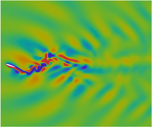
Figure 10 presents a comparison of typical field patterns for velocity and pressure between the stratified case at $Fr = 3.5$ and homogeneous flow. From a distant viewpoint, it can be seen that the oscillating foil in the homogeneous flow generates alternating wake structures along the centreline (see figure 10$a$,$b$), which are less apparent in the stratified flow (see figure 10$d$,$e$). Instead, in the stratified regime, wave beams can be clearly identified in both the velocity and pressure fields due to the induced internal waves. These wave beams are found to propagate in all directions, giving rise to a flow pattern that covers the entire domain. The effective angle of attack, determined by the combination of foil kinematics and flow conditions, is a dominant parameter that affects the force characteristics of an oscillating foil. As shown in figures 10($d$) and 10($e$), the stratification effect is found to recompose the velocity of incoming flow, suggesting a change in resulting effective angle of attack. In contrast with the typical pressure field in a homogeneous flow (see figure 10$c$), the specific pressure distribution around the oscillating foil under stratification influence, as seen in figure 10($\,f$), definitely contributes to the aforementioned force behaviours in the stratified flow. Therefore, we conjecture that the enhancement of force production in the stratified realm can be attributed to two reasons: the change in incoming flow conditions improving the effective angle of attack and the formation of a favourable pressure field that benefits the pressure distribution along the foil surface.

Figure 10.

Contour plots of the instantaneous velocity and pressure fields from a distant viewpoint for an oscillating foil with ${\alpha _0} = 15^\circ$ in (a–c) homogeneous flow and (d–f) stratified flow at $Fr = 3.5$. The velocity and pressure are normalised by ${U_\infty }$ and ${\rho _0}U_\infty ^2$, respectively. The snapshot corresponds to the instant when the oscillating foil moves through the centreline after an oscillation cycle ($t = T$).

We first explore the formation of a favourable pressure field in the stratified regime. The pressure distribution around an oscillating foil with ${\alpha _0} = 15^\circ$ is presented in figure 11, which includes four representative stratified cases along with the homogeneous scenario. We consider the instant of $t = 3/8T$ here, corresponding to the noticeable disparity in the instantaneous force coefficients between the homogeneous and stratified results (see figure 8). In the homogeneous flow, the oscillating foil generally encounters a high-pressure region on the lower surface of the leading edge during the downstroke motion, accompanied by a low-pressure region around the upper surface of the foil, as illustrated in figure 11($e$). The pressure field around the trailing edge is characterised by a series of low-pressure regions resulting from vortex shedding. When introducing a weak stratification, as shown in figure 11($d$), the low-pressure region around the trailing edge in the homogeneous flow is displaced by a wide high-pressure region that approximately covers half the foil surface. With the increase in stratification strength, the newly formed high-pressure region tends to approach the rear of the foil, becoming more concentrated and intense. Consequently, a high-pressure region in the form of a slender tail pinned at the trailing edge of the oscillating foil is observed in figure 11($a$–$c$). This pressure distribution generates a considerable horizontal pressure difference, directing force towards the advancement, thus amplifying thrust production.

Figure 11.

Detailed distribution of the instantaneous velocity field and pressure contour normalised by ${\rho _0}U_\infty ^2$ around the oscillating foil with ${\alpha _0} = 15^\circ$ for (a) $Fr = 1.0$, (b) $Fr = 2.5$, (c) $Fr = 3.5$, (d) $Fr = 8.0$ and (e) $Fr = \infty$ (homogeneous flow). The snapshot corresponds to the instant of $t = 3/8T$ during the downstroke of an oscillation cycle. The zoom-in results at the lowest row illustrate the comparison of free stream velocity vectors near the leading edge of the oscillating foil between homogeneous scenario and stratified case of $Fr = 3.5$.

Moreover, as the stratification strength increases, the upper and lower surfaces of the foil are enveloped by two narrowed low-pressure regions. During the downstroke oscillation, the upper low-pressure region exhibits a wider range and lower pressure intensity than that on the lower foil surface, leading to a suction force on the upper surface, thereby contributing to lift generation. This mechanism mirrors during the upstroke oscillation, where the suction force acts on the lower foil surface.

The emergence of such a favourable pressure field, which enhances the force production in stratified flows, stems from the momentum redistribution facilitated by induced internal waves and the confined impact on the vertical evolution of flow structures due to the restoring force of buoyancy. Unlike the homogeneous scenario, where fluid motion is primarily driven by boundary stresses or flow instabilities, dynamics in the stratified realm largely arise from the transfer of energy and momentum through internal waves (Ivey et al. Reference Ivey, Winters and Koseff2008; Dauxois et al. Reference Dauxois, Joubaud, Odier and Venaille2018). Consequently, the pressure distribution around the oscillating foil tends to follow the path of wave propagation, resulting in the distinct pressure field observed. Moreover, aside from radiating as internal waves, energy is diverted into horizontal advective motions within stratified flows, aiding the streamwise development of vortices (Godoy-Diana et al. Reference Godoy-Diana, Chomaz and Donnadieu2006). Hence, the suppression of vertical movements, coupled with the promotion of horizontal flow structures, leads to the stretched and compressed pressure profiles evident in the stratified regime.

We subsequently investigate the alterations in incoming flow conditions induced by stratification. The velocity fields around an oscillating foil at ${\alpha _0} = 15^\circ$ are depicted in figure 11. Specifically, the bottom contour plots provide a detailed comparison of velocity vectors near the foil's leading edge between the homogeneous scenario and the stratified case at $Fr = 3.5$. The circled regions indicate that the influence of density stratification on the incoming velocity field is primarily characterised by changes in flow direction, while the magnitude of velocity vectors remains nearly constant compared with the homogeneous flow. For an oscillating foil during the downstroke motion, the stratified effect tends to deflect the velocity direction of the incoming flow upward. This deflection significantly affects the behaviour of the foil boundary layer, considering that the angle of attack required to trigger dynamic stall has a threshold of approximately $20^\circ$ to $25^\circ$ in the homogeneous flow, depending on the kinematics (Akbari & Price Reference Akbari and Price2003).

Figure 12 illustrates the dependence of instantaneous force characteristics on the change of incoming flow conditions. We adopt an analysis strategy similar to that of Muscutt et al. (Reference Muscutt, Weymouth and Ganapathisubramani2017), who studied the effects of the vortex-induced velocities by the fore foil on the force generation of the hind foil in a tandem configuration. Here, we use subscripts $h$ and $s$ to denote the homogeneous and stratified cases, respectively. The decomposed drag and lift resulting from the effective velocity are denoted as $D$ and $L$, respectively. Based on the observations in figure 11, we assume that the velocity of incoming flow in the stratified regime has a deflected angle $\sigma$ relative to the homogeneous free stream flow, while their magnitudes remain the same. Compared with the homogeneous flow, the stratification effect leads to a decrease in the streamwise velocity component ($\Delta u$) but induces a cross-flow velocity component ($\Delta v$). Since the cross-flow component of the stratification-induced velocity ($\Delta v$) shares the same direction as the heave velocity of the oscillating foil ($\mathrm {d}h(t)/\mathrm {d}t$), the magnitude of the resultant velocity in the stratified flow gains an increase, suggesting the enhancement of thrust production at the considered instant. In addition, the combined effect of $\Delta u$ and $\Delta v$ results in a higher effective angle of attack in the stratified regime, consequently increasing lift production. We note that the same directional relationship between $\Delta v$ and $\mathrm {d}h(t)/\mathrm {d}t$, as well as the behaviour of ${\alpha _s} > {\alpha _h}$, are observed during both the downstroke and upstroke motions due to the periodicity of kinematics, indicating the augmentation of forces throughout the entire oscillation cycle. We further observe a less significant variation in the deflected angle $\sigma$ as the stratification level increases. Therefore, we believe that, compared with the formation of favourable pressure fields, the change of incoming flow conditions plays a secondary role in enhancing force production in the stratified regime.

Figure 12.

Schematic illustration of the influence of velocity components induced by the stratification effect on the force characteristics of an oscillating foil.

4.2. Effect of maximum angle of attack

The specific ${\alpha _0}$ for a given parameter combination is derived by adjusting ${\theta _0}$ in (2.4). Figure 13 displays the time-dependent variation of the angle of attack over one oscillation cycle with different ${\alpha _0}$, stemming from (2.3). It is notable that the angle of attack profiles at ${\alpha _0} = 5^\circ$ and $10^\circ$ exhibit multiple peaks per cycle, attributed to the presence of high-order harmonics in the first term on the right-hand side of (2.3) (Read et al. Reference Read, Hover and Triantafyllou2003). Consequently, the actual ${\alpha _0}$ slightly exceeds the desired value for these cases. While this deviation in the angle of attack profile could be rectified by adjusting the foil motion, our study demonstrates that the observed degradation in the angle of attack is negligible, as depicted in figure 13. Hence, there is no necessity to modify the foil motion. Our main focus lies in examining the varying dependence of propulsive performance on the maximum angle of attack across different stratification levels. Notably, the low sensitivity to ${\alpha _0}$ observed at transitional stratifications is of particular interest.

Figure 13.

Instantaneous effective angle of attack over one periodic cycle for different ${\alpha _0}$.

Figures 14–18 display the instantaneous thrust and lift coefficients with different maximum angles of attack for four stratified cases and the homogeneous scenario. We can see that both the thrust and lift coefficients tend to achieve their peaks immediately after the highest effective angle of attack is reached. In the homogeneous case, the peak of the time-dependent lift coefficient exhibits a monotonically increasing trend with increasing ${\alpha _0}$, while the maximum instantaneous thrust coefficient occurs at ${\alpha _0} = 25^\circ$. The influence of ${\alpha _0}$ on the time evolution of force characteristics is significant throughout the entire oscillation cycle in the homogeneous flow (see figure 14). For the case of $Fr = 8.0$, the force profiles as a function of ${\alpha _0}$ bear a striking resemblance to the homogeneous results (see figure 15), indicating the dominance of kinematics at weak stratifications. Owing to that, the high dependence of propulsive performance on the maximum angle of attack is observed in the weakly stratified flow.

Figure 14.

Effect of the maximum angle of attack on the time-dependent (a) thrust coefficient and (b) lift coefficient in the homogeneous flow ($Fr = \infty$).

Figure 15.

Effect of the maximum angle of attack on the time-dependent (a) thrust coefficient and (b) lift coefficient at the stratification level of $Fr = 8.0$.

Figure 16.

Effect of the maximum angle of attack on the time-dependent (a) thrust coefficient and (b) lift coefficient at the stratification level of $Fr = 3.5$.

Figure 17.

Effect of the maximum angle of attack on the time-dependent (a) thrust coefficient and (b) lift coefficient at the stratification level of $Fr = 2.5$.

Figure 18.

Effect of the maximum angle of attack on the time-dependent (a) thrust coefficient and (b) lift coefficient at the stratification level of $Fr = 1.0$.

As the stratification strength is further increased to moderate ($Fr = 3.5$) and transitional ($Fr = 2.5$) levels, the time-dependent forces show more complex behaviours with varying ${\alpha _0}$, as depicted in figures 16 and 17. These behaviours clearly deviate from the homogeneous counterpart. Specifically, the role of ${\alpha _0}$ is found to be less significant during the first quarter cycle, after which its impact tends to be amplified in the second quarter cycle. We note that the peak thrust production at $Fr = 2.5$ occurs at ${\alpha _0} = 30^\circ$, in contrast to the stratified case of $Fr = 3.5$ and the homogeneous case, both of which yield the highest thrust coefficient at ${\alpha _0} = 25^\circ$. This distinction suggests that the oscillating foil experiences different dynamic-stall events at the stratification level of $Fr = 2.5$ compared with the other two cases.

Figure 18 illustrates that the instantaneous force characteristics at strong stratifications exhibit a sinusoidal-like profile resembling the results obtained in the homogeneous case, albeit with a certain phase difference. Our observations regarding flow patterns suggest that the boundary-layer behaviours are predominantly influenced by the induced internal waves under the strong stratifications, where the foil kinematics play an insignificant role. Referring to the results presented in figure 5, the decline in propulsive efficiency at $Fr = 1.0$ with increasing ${\alpha _0}$ mainly stems from the surge in required power. The peak lift coefficient at $Fr = 1.0$ as a function of the maximum angle of attack exhibits a notable increasing trend for ${\alpha _0} \le 25^\circ$, followed by a slight decrease with a plateau of high-scale lift generation at ${\alpha _0} = 30^\circ$, which gives rise to the surge of input power. We attribute the lift augmentation with the maximum angle of attack under strong stratifications to two potential reasons. First, a higher ${\alpha _0}$ indicating a less stable boundary layer can enhance the induction of internal waves. Second, since the desired ${\alpha _0}$ is achieved by adjusting the pitching magnitude ${\theta _0}$ in our computations, a high ${\alpha _0}$ actually corresponds to a low ${\theta _0}$, which tends to alleviate the viscous diffusion of induced internal waves around the oscillating foil. Both behaviours can strengthen the wavelike flow patterns and lead to a longer duration of flow structures near the foil, contributing to the lift augmentation. As a consequence, the optimum propulsive efficiency under strong stratifications is achieved at the lowest ${\alpha _0}$.

Considering the vertical inhibition of boundary-layer evolution by stratification effect and aforementioned force characteristics in the stratified flow, it is reasonable to associate the low sensitivity to ${\alpha _0}$ at $Fr = 2.5$ with dynamic-stall events. It should be noted that we cannot determine whether the dynamic stall occurs or not based on figures 14 to 18 because the presented force coefficients (${C_t}$ and ${C_l}$) only represent the superposition of streamwise and cross-flow projection components of lift and drag induced by the effective velocity (see figure 12). Dynamic stall refers to the phenomenon that the onset of stall for an airfoil executing unsteady motion is delayed to angles significantly exceeding the static-stall angle (Carr Reference Carr1988). The occurrence of dynamic stall is accompanied by a sudden decrease in lift and a rapid increase in drag, indicating a reduction in thrust production and an increase in input power for an oscillating foil. Thus, we can qualitatively identify the onset of dynamic stall by observing the degradation of cycle-averaged performance for a combined heaving and pitching foil (Isogai, Shinmoto & Watanabe Reference Isogai, Shinmoto and Watanabe1999). Figure 19 compares the cycle-averaged propulsion characteristics in stratified flows at $Fr = 2.5$ and 3.5 with the homogeneous counterpart. It is evident that the increasing trend of thrust production observed in the homogeneous flow markedly slows down when the maximum angle of attack exceeds $16.3^\circ$, whereas this threshold extends to $24.5^\circ$ for the stratified case of $Fr = 3.5$. Throughout the entire range of ${\alpha _0}$ considered, the cycle-averaged thrust coefficient shows a monotonic increase for $Fr = 2.5$ (see figure 19$a$), indicating that the threshold angle of attack triggering dynamic-stall events in the stratified flow is higher than that in the homogeneous flow. This feature becomes even more prominent when examining the variation of propulsive efficiency, as shown in figure 19($b$). To assess the sequence of dynamic stall onset for the three considered cases, we introduce a parameter ${\alpha _{te}}$ that represents the threshold maximum angle of attack beyond which the efficiency starts to deteriorate. Although ${\alpha _{te}}$ does not precisely quantify the stalling angle of an unsteady heaving and pitching foil, it provides a qualitative indication for the dynamic-stall onset. Our results indicate that the ${\alpha _{te}}$ values corresponding to $Fr = \infty$ (homogeneous), $Fr=3.5$ and $Fr=2.5$ are $14.3^\circ$, $17.2^\circ$ and $21.1^\circ$, respectively. This behaviour signifies that an oscillating foil in the homogeneous flow first experiences dynamic-stall events as the maximum angle of attack continuously increases, followed by dynamic stall occurring at the stratification level of $Fr = 3.5$. The propulsion performance in the stratified flow with $Fr = 2.5$ exhibits the highest tolerance for the effective angle of attack, as it requires the highest ${\alpha _0}$ to trigger dynamic stall among the three cases.

Figure 19.

Variation of the (a) time-averaged thrust coefficient and (b) propulsive efficiency as a function of the maximum angle of attack for both homogeneous flow and stratified cases at $Fr = 2.5$ and 3.5. The parameter ${\alpha _{te}}$ represents the threshold value of the maximum angle of attack, beyond which the propulsive performance begins to decline.

Inherently, the dynamic stall results from massively separated unsteady flow. The significant variations in propulsion performance of an oscillating foil, particularly during dynamic stall, primarily arise from the occurrence of leading-edge flow separation. This behaviour is typified by the formation, convection and shedding of a vortex at the leading-edge region, inducing nonlinear fluctuation in pressure distribution and transient alterations in force characteristics (Carr Reference Carr1988; Akbari & Price Reference Akbari and Price2003; Lee & Gerontakos Reference Lee and Gerontakos2004). In light of this, we explore the mechanism that gives rise to the delay of dynamic stall in the stratified regime by examining the vortex characteristics around the oscillating foil. Figure 20 presents the instantaneous contour plots of the vorticity field for three distinct cases. Specifically, we focus on the instant of $t = T/8$ when substantial flow separation becomes evident over one oscillation cycle. The maximum angles of attack considered, namely ${\alpha _0} = 15^\circ$, $25^\circ$ and $30^\circ$, encompass the transition from an attached boundary layer to a fully separated flow in the homogeneous case.

Figure 20.

Comparison of instantaneous vorticity contours between homogeneous flow and stratified cases at $Fr = 2.5$ and 3.5 for (a) ${\alpha _0} = 15^\circ$, (b) ${\alpha _0} = 25^\circ$ and (c) ${\alpha _0} = 30^\circ$. The vorticity field is visualised using red and blue colours to represent positive (anticlockwise) and negative (clockwise) values, respectively, with contour levels ranging from $-$5 to 5, normalised by ${U_\infty }/c$. The snapshot corresponds to the instant of $t = 1/8T$ during the upstroke of the oscillation cycle.

Our findings indicate that the leading-edge flow separation is greatly inhibited by density stratification, resulting in a heightened threshold angle of attack necessary to trigger dynamic-stall events in stratified flows. At ${\alpha _0} = 15^\circ$, we observe that the boundary layer remains largely attached across all three cases, except for a thin layer of flow reversal (FR) detected at the lower surface of the oscillating foil in the homogeneous flow, as depicted in the inset of figure 20($a$). This flow reversal, emanating from the rear and progressing towards the front, signifies an effective angle of attack surpassing the static-stall angle, instigating the subsequent development of leading-edge vortices (LEVs) (Lee & Gerontakos Reference Lee and Gerontakos2004). In contrast, the unsteady boundary layer in the stratified flow exhibits greater stability compared with its homogeneous counterpart, with the absence of the flow reversal phenomenon in the cases of $Fr = 2.5$ and 3.5.

Increasing the maximum angle of attack to ${\alpha _0} = 25^\circ$ results in prominent leading-edge separation (LE-S) in the homogeneous flow. However, in the stratified scenario with $Fr = 3.5$, the disturbance in the boundary layer at the foil's front is delayed towards the rear, manifesting as a trailing-edge separation (TE-S) with reduced extent (see figure 20$b$). Surprisingly, at a stratification level of $Fr = 2.5$, the boundary layer around the oscillating foil remains attached even at ${\alpha _0} = 25^\circ$. Elevating the maximum angle of attack to ${\alpha _0} = 30^\circ$ in the homogeneous flow leads to extensive LE-S accompanied by significant vortex shedding from the foil's front, as displayed in figure 20($c$). In contrast, both stratified cases of $Fr = 2.5$ and 3.5 at ${\alpha _0} = 30^\circ$ exhibit a tendency to delay boundary-layer instability growth and shift the separation point towards the foil's rear. This results in a prolonged duration of vortex presence over the foil surface, consequently culminating in trailing-edge flow separation (see figure 20$c$). Notably, the intensity and extent of flow separation, along with the distance between the separation point and the foil's trailing edge, diminish as the stratification strength increases.

Therefore, density stratification emerges as a significant stabilising factor for boundary-layer motion, facilitating the shift from extensive leading-edge flow separation observed in homogeneous flows to restricted trailing-edge flow separation in the stratified regime. The stabilising influence on flow structure evolution in the stratified regime has been widely acknowledged through both numerical simulations and experimental measurements (Boyer et al. Reference Boyer, Davies, Fernando and Zhang1989; Godoy-Diana et al. Reference Godoy-Diana, Chomaz and Donnadieu2006; Chongsiripinyo et al. Reference Chongsiripinyo, Pal and Sarkar2017). Owing to this mechanism, dynamic-stall occurrences in an oscillating foil are notably mitigated and delayed within the stratified flow, which accounts for the diminished dependence of propulsion performance on the maximum angle of attack in transitional stratifications. These findings hold promise in providing valuable insights into flow control strategies, particularly concerning vortex manipulation and mitigation of extensive separation.

5.1. Vortex structures

We begin by investigating the influence of stratification on the spatiotemporal characteristics of vortex topology. Figure 21 presents the wake patterns characterised by vortex structures for four representative stratification levels, with the homogeneous case serving as a reference frame. We consider three maximum angles of attack: ${\alpha _0} = 5^\circ$, $15^\circ$ and $25^\circ$, which span the range from an attached boundary layer to a massively separated flow in the homogeneous case. It can be seen that the tightly attached boundary layer in the homogeneous flow with ${\alpha _0} = 5^\circ$ results in a smooth shedding of vortices from the trailing edge of the oscillating foil, whereas the LEV plays a minor role in the wake formation. As the detached trailing-edge vortex (TEV) advects farther downstream, it bifurcates into two segments, leading to a 2P wake mode. At an increasing ${\alpha _0}$, the wake undergoes a transition from the 2P mode to the 2S reverse von Kármán mode in the homogeneous flow, as observed in figure 21($b$,$c$). This transition is attributed to the growing influence of the LEV on wake structures.

Figure 21.

Instantaneous vorticity contours at different stratification levels for (a) ${\alpha _0} = 5^\circ$, (b) ${\alpha _0} = 15^\circ$ and (c) ${\alpha _0} = 25^\circ$. The vorticity field is represented by red and blue colours for positive (anticlockwise) and negative (clockwise) values, respectively, with contour levels ranging from $-$1.25 to 1.25, normalised by ${U_\infty }/c$. The snapshot corresponds to the instant when the oscillating foil crosses the centreline after completing an oscillation cycle ($t = T$).

Several distinct wake patterns that significantly differ from the observations in the homogeneous flow are identified in the stratified regime. For a weak stratification ($Fr = 8.0$), the wake pattern exhibits a triangular configuration, in which a central wake advects along the centreline and two symmetric oblique wakes deflect from the centreline. Particularly, at relatively high ${\alpha _0}$ values, we observe an exotic vortex package structure characterised by a well-formed core vortex encircled by other stretched vortices (see figure 21$c$). The moderate ($Fr = 3.5$) and transitional ($Fr = 2.5$) stratifications produce a downstream-radial wake configuration, where vortex perturbations travel in all directions with a dominant downstream advection. We note that, as the maximum angle of attack increases, the interactions between vortices become more pronounced, leading to the distortion and splitting of vortex structures. Consequently, a relatively chaotic region can be seen in the near wake of the oscillating foil. In contrast to the vortex package identified at $Fr = 8.0$, increasing the stratification level to such an extent produces multiple dipole-like pairs consisting of counter-rotating vortices with comparable circulation strength. For strong stratifications ($Fr = 1.0$), the wake arrangement shows an upstream-radial pattern, in which the vortex perturbations spread towards all directions with a dominant upstream advection. This upstream dominance of vortex topology becomes more pronounced as the maximum angle of attack increases. At such high stratification levels, wave–vortex interactions become prominent, resulting in a significantly disordered near wake and a less visible far wake.

The formation and evolution of the upstream-radial configuration at strong stratifications are indicated to be determined by induced internal waves principally, with a low dependence on foil kinematics and boundary layer roll-up. We will provide more details regarding the behaviours of internal waves in subsequent subsections. Here, we focus our attention on the characteristics of the triangular wake pattern at weak stratifications and the downstream-radial wake arrangement at transitional and moderate stratifications. We specifically consider the scenario with ${\alpha _0} = 25^\circ$, since both the vortex topology and wake pattern are more discernible at a higher maximum angle of attack.

To provide a basis for reference, we briefly outline the formation process of the 2S reverse von Kármán vortex street in the homogeneous flow, as depicted in figure 22. Here, superscripts $a$ and $b$ denote the previous and current oscillation cycles, respectively. When the oscillating foil moves away from the mean position during the upstroke motion, the roll-up of the boundary layer induces a lower-surface LEV (LEV${1^b}$). At $t = T/4$, the LEV${1^b}$ grows close to the point of detachment (see figure 22$b$). During the following downstroke oscillation, the LEV${1^b}$ is shed from the midchord position of the oscillating foil, accompanied by the detachment of a TEV in the same sense of rotation (see figure 22$c$). Due to its relatively low circulation strength and small size compared with the LEV${1^b}$, the TEV merges into the LEV${1^b}$ in the subsequent advection. As the foil further moves downward, a new LEV (LEV${2^b}$) forms on the upper surface of the oscillating foil. It experiences a similar process of development and evolution as the LEV${1^b}$. As a result, two primary LEVs are shed into the wake per oscillation cycle, generating a reverse von Kármán vortex street. Such a wake configuration creates a momentum surplus, indicating thrust production.

Figure 22.

Contour plots of the instantaneous vorticity field, depicting the wake evolution in the homogeneous flow for ${\alpha _0} = 25^\circ$ during one oscillation cycle. The positive (anticlockwise) and negative (clockwise) vorticity values are represented by red and blue colours, respectively. The contour levels range between $-$2 and 2, normalised by ${U_\infty }/c$.

We now examine the formation process of wake patterns in stratified flows. Figure 23 shows the temporal evolution of vortex topology at the stratification level of $Fr = 8.0$. The primary feature of the triangular flow pattern produced by such a weak stratification is the formation of a distinctive vortex package, as highlighted by the black dashed square in figure 23($a$). Since the development of this vortex package takes a longer period of time than one oscillation cycle, we track the vortices shed in the previous cycle of foil motion. The creation of the vortex package begins with the interaction between the LEV${2^a}$ shed from the upper foil surface and the TEV${2^a}$ detached from the lower foil surface, as depicted in figure 23($a$). Due to their opposite sense of rotation and unequal circulation strength, the LEV${2^a}$ is enveloped by the TEV${2^a}$ that undergoes significant distortion due to the combined effects of vortex interactions and internal waves (see figure 23$b$,$c$). Meanwhile, a mutual induced vortex (MIV) (MIV${2^a}$) forms in the downstream wake region, resulting from the previous-cycle detached TEV coupled with the inductive effect of wave propagation (see figure 23$a$). As the LEV${2^a}$ advects downstream, the TEV${2^a}$ splits into two parts, while the MIV${2^a}$ continues to grow in both size and strength (see figure 23$d$). With the wake evolution proceeding, the intertwined LEV${2^a}$ and TEV${2^a}$ approach the MIV${2^a}$ due to their relatively high advecting velocity (see figure 23$e$–$g$). Consequently, the broken TEV${2^a}$ and fully developed MIV${2^a}$ forms a protective circle around the LEV${2^a}$ (see figure 23$h$). Owing to this protection effect, the LEV${2^a}$ retains its intact shape throughout the entire formation process of the vortex package, in contrast to the stretched TEV${2^a}$ and MIV${2^a}$. This vortex package dissipates within a short period of time due to intense energy exchange and transport by internal waves. In further evolution, the LEV${2^a}$ and MIV${2^a}$ with the same sense of rotation merge into a single vortex structure advecting along the centreline, which eventually forms the central wake. Simultaneously, the TEV${2^a}$ pairs with the neighbouring vortex detached from the trailing edge after the shedding of LEV${2^a}$, forming a dipole-like structure that contributes to the formation of the oblique wake away from the centreline. It has been indicated that the mutual induced velocity of the dipole-like structure in the transverse direction is the main cause of the wake bifurcation (Schnipper et al. Reference Schnipper, Andersen and Bohr2009; Verma & Hemmati Reference Verma and Hemmati2022). The formation process of the vortex package centred on the LEV${1^a}$ follows a similar pattern, with the involved vortices rotating in the opposite direction.

Figure 23.

Contour plots of instantaneous vorticity field depicting the wake evolution in the stratified flow with a stratification level of $Fr = 8.0$ for ${\alpha _0} = 25^\circ$ during one oscillation cycle. The positive (anticlockwise) and negative (clockwise) vorticity values are represented by red and blue colours, respectively. The contour levels range between $-$2 and 2, normalised by ${U_\infty }/c$. The time series of flow structures, highlighted by white dashed circle, demonstrates the formation of a vortex package.

It is essential to provide additional details regarding the above-mentioned MIV, since this particular vortex structure is not observed in homogeneous flows. Figure 24 depicts the arising region of a typical MIV in relation to the advecting profile of internal waves at $t = T/2$, as marked by the yellow dashed ellipse. It is evident that both the position and shape of the MIV closely coincide with the propagating pattern of internal waves, in which the wave crests and troughs are highlighted by black lines. This alignment persists throughout the entire evolution process of the wake. Considering the fact that unsteady oscillations in a stratified flow trigger multiple momentum transfers and energy exchanges between wave and mean flow (Godoy-Diana et al. Reference Godoy-Diana, Chomaz and Donnadieu2006), we attribute the creation and development of the MIV to the reorganisation of the TEV, which is shed during the previous half-oscillation-cycle. This reorganisation occurs through a disturbance-transport mechanism that involves energy exchange between advective vortices, propagating internal waves and background mean flow. Figure 24 also provides a more vivid depiction of the triangular flow pattern, wherein two oblique wakes bifurcate from the central wake at a certain angle.

Figure 24.

Instantaneous vorticity contour normalised by ${U_\infty }/c$, indicating the position of onset of a MIV in relation to the propagating pattern of internal waves. The crests and troughs of the wave pattern are marked by black solid and dashed lines, respectively. The snapshot corresponds to the instant when the oscillating foil crosses the centreline after completing half an oscillation cycle ($t = T/2$).

For the downstream-radial flow pattern at moderate and transitional stratifications, we examine the temporal evolution of wake characteristics behind an oscillating foil at $Fr = 3.5$, as shown in figure 25. The dominant feature observed is the significant interaction of vortices in the near wake. The complete formation process of the downstream-radial wake can be roughly divided into two phases. In the first phase, the interaction between LEV and TEV prevails, as indicated by the white dashed square. As the oscillation approaches $t = T/4$, the developed LEV${1^b}$ detaches from the lower surface of the trailing edge, while the TEV${1^b}$ is simultaneously shed from the opposite side of the foil (see figure 25$c$). With the advection proceeding, both the LEV${1^b}$ and TEV${1^b}$ split into two parts when they become entangled with each other (see figure 25$e$). Due to the dominance of the LEV${1^b}$ in terms of circulation strength and size, the TEV${1^b}$ is dissipated rapidly by the counter-rotating LEV${1^b}$ that constitutes the central wake during further advection (see figure 25$f$). The second phase, indicated by the white dashed ellipse, involves the mutual interaction of TEVs shed from opposite sides of the foil with MIVs. This phase begins with the detachment of two elongated vortex structures from the trailing edge (see figure 25$e$), followed by an intertwined course between these vortices (see figure 25$f$). Meanwhile, numerous newly formed MIVs join this intertwined course, involving multiple processes of vortex breaking and merger, as well as energy exchange and dissipation. Consequently, a cluster of isolated vortex structures are generated, contributing to a markedly disordered near wake (see figure 25$g$). These isolated vortices further advect to feed the formation of oblique wakes. At higher stratification levels, the influence of induced internal waves on the flow pattern becomes increasingly dominant, indicating a more pronounced wave–vortex momentum exchange. Compared with the wake evolution at a weak stratification (see figure 23), it can be seen that a considerable number of MIVs develop and involve in the formation process of the downstream-radial flow pattern (see figure 25), although they are not explicitly marked for clarity. The increasing dominance of induced internal waves are believed to enable the spreading of vortex disturbance towards the upstream direction, leading to a radial pattern. In addition, the formation of multiple dipole-like structures during the vortex interactions induces transverse and upstream velocities, partially contributing to the formation of the radial flow configuration.

Figure 25.

Contour plots of the instantaneous vorticity field illustrating the wake evolution in the stratified flow with a stratification level of $Fr = 3.5$ for ${\alpha _0} = 25^\circ$ during one oscillation cycle. The vorticity contours are denoted by red and blue colours, indicating positive (anticlockwise) and negative (clockwise) values, respectively. The contour levels range from $-$2 to 2, normalised by ${U_\infty }/c$. The time series of flow structures, highlighted by a white dashed square and ellipse, illustrate the mutual interaction of shedding and induced vortices.

The intense vortex interactions observed at $Fr = 3.5$ in figure 25 are attributed to the relatively high advection velocity of shed vortices, resulting from the compressing effect along the gravitational direction and the pushing effect towards the streamwise direction of density stratification. Figure 26 shows the time evolution of the LEV${1^b}$ position along the streamwise direction over one oscillation cycle for three cases. It can be observed that the LEV${1^b}$ moves slowly at the initial stage since it is still attached to the foil surface. The advection velocity remains nearly constant after the LEV${1^b}$ completely detaches from the oscillating foil, when $t \ge 0.4T$. We thus define the phase speed ${U_{phase}}$ of the LEV${1^b}$ as the mean velocity calculated within the period of time from $t = 0.4T$ to $T$. In the homogeneous flow, ${U_{phase}}$ is found to be smaller than ${U_\infty }$ in the near wake, as the LEV${1^b}$ experiences a slight acceleration process in the initial part of the wake. When we calculate the advection velocity of LEV${1^b}$ from the streamwise position five chord lengths downstream of the leading edge, ${U_{phase}}/{U_\infty }$ increases to 1.05, in agreement with the propulsive nature of the reverse von Kármán wake associated with ${U_{phase}} > {U_\infty }$ (Godoy-Diana et al. Reference Godoy-Diana, Marais, Aider and Wesfreid2009). In the stratified flow with a weak stratification ($Fr = 8.0$), the LEV${1^b}$ exhibits a slightly higher advection velocity compared with the homogeneous case. However, the phase speed of the LEV${1^b}$ in the stratified case of $Fr = 3.5$ remarkably increases by $27.6\,\%$ to a significant level of ${U_{phase}}/{U_\infty } = 1.34$, indicating an energetic momentum jet in the near wake of the oscillating foil. Thus, enhancing the phase velocity of vortices by a sufficiently high stratification level emerges as an important mechanism responsible for the significant performance at moderate stratifications.

Figure 26.

Time-dependent streamwise position of LEV${1^b}$ in the near wake of the oscillating foil for the cases of homogeneous flow and stratified flows with $Fr = 3.5$ and 8.0. The starting point of $t = 0$ corresponds to the instant when the oscillating foil crosses the centreline before the upstroke motion. The horizontal axis originates from the initial position of the foil's leading edge with zero pitching angle. The advection velocity of LEV${1^b}$ in the far wake of the oscillating foil for the homogeneous case is calculated based on the horizontal position five chord lengths downstream of the leading edge, with a travel distance of 10 chord lengths.

5.2. Streamwise jet patterns

We present an evaluation on the characteristics of time-averaged streamwise velocity to gain insights into the propulsion enhancement in stratified flows. Figure 27 illustrates the mean velocity profiles for four representative stratification levels, as well as the homogeneous counterpart. These profiles are obtained at a location two chord lengths downstream of the trailing edge to quantitatively examine the near-wake features. Accordingly, figure 28 shows the contour plots of the time-averaged streamwise velocity fields. We consider the homogeneous scenario as a reference case here. The findings reveal that, as the maximum angle of attack increases, the near-wake velocity within the homogeneous flow undergoes a notable transition from a multipeak profile to a plateau with a single-peak configuration, as depicted in figure 27($a$). This observed behaviour corresponds to the alterations in the velocity fields shown in figure 28. It can be seen that two diverging velocity excess streams at ${\alpha _0} = 5^\circ$ are merged into a broad and intense velocity jet at ${\alpha _0} = 25^\circ$, which results from the wake transition from 2P mode to 2S reverse von Kármán arrangement at an increasing maximum angle of attack (see figure 21).

Figure 27.

Profiles of the time-averaged streamwise velocity, normalised by ${U_\infty }$, for different maximum angles of attack, corresponding to the stratification levels of (a) $Fr = \infty$ (homogeneous flow), (b) $Fr = 8.0$, (c) $Fr = 3.5$, (d) $Fr = 2.5$ and (e) $Fr = 1.0$. The data is extracted along the cross-stream line at a streamwise location two chord lengths downstream of the trailing edge.

Figure 28.

Contours of the time-averaged streamwise velocity field, normalised by ${U_\infty }$, at different stratification levels for (a) ${\alpha _0} = 5^\circ$, (b) ${\alpha _0} = 15^\circ$ and (c) ${\alpha _0} = 25^\circ$. A reference scale of $5c$ is added to the first plot to indicate the field dimensions. The left-hand border of each plot corresponds to the initial position of the trailing edge.

Given the observations of vortex structures, we anticipate that the jet patterns in the stratified flow differ significantly from the homogeneous characteristics described above. Figure 27($b$) shows that the weak stratification ($Fr = 8.0$) at a small maximum angle of attack produces a double-peak velocity profile along the wake centreline, which converges into a single-peak jet with an evident increase in velocity magnitude as ${\alpha _0}$ increases. The velocity distribution away from the centreline follows a wave-like pattern in the form of alternating velocity minima and maxima with attenuating magnitudes. Figure 28 shows that the velocity field in the stratified flow exhibits a radial pattern, manifesting as a centreline jet clamped by multiple diverging deficit and excess streams that resemble wave beams. As the stratification strength increases to $Fr = 3.5$, there is an increasing trend in the number of velocity minima and maxima alternately appearing on both sides of the centreline, as shown in figure 27($c$). This behaviour is confirmed by the velocity field of $Fr = 3.5$ (see figure 28), where the diverging streams of radial velocity configuration become denser. At $Fr = 2.5$, a double-peak velocity profile is observed around the central near-wake region for all three maximum angles of attack (see figure 27$d$). Notably, the difference in peak velocity along the wake centreline with the variation of ${\alpha _0}$ is found to be insignificant for $Fr = 2.5$. This observation aligns with the aforementioned low dependence of propulsion performance on the maximum angle of attack at transitional stratifications. Figure 28 demonstrates the presence of an evident velocity deficit region in the near wake of $Fr = 2.5$, corresponding to the double-peak velocity profile in figure 27($d$). When the stratification level increases to $Fr = 1.0$, the near-wake velocity profile along the centreline is characterised by a single-peak jet (see figure 27$e$). The velocity distribution on both sides of the wake centreline indicates a considerable complexity under strong stratifications. Figure 28 reveals a cluster of highly concentrated velocity streams centred on a finite high-intensity jet in the near wake of mean velocity field for $Fr = 1.0$.

The formation of the radial velocity pattern, as depicted in figure 28, can be attributed to the mutual induction of vortex structures in stratified flows. The velocity jet along the centreline is induced by the central reverse von Kármán wake, which consists of two sequences of coherent vortex structures (see figure 21). The interaction between a row of vortex structures from the central wake and the neighbouring vortex sequence from the oblique wake leads to a normal von Kármán vortex street (see figure 24), resulting in the velocity deficit region on each side of the centreline. The vortex distribution in the form of a wave-like pattern induces resultant velocities along the interface between crests and troughs of the vorticity field (see figure 21), generating multiple diverging velocity streams and thus giving rise to a radial arrangement. The mean velocity field in the stratified flow generally exhibits two prominent characteristics in terms of spatial arrangement. First, it is observed that the central velocity jet is compressed along the cross-flow direction due to the restoring force of buoyancy. Second, the region of maximum velocity along the wake centreline is found to move towards the trailing edge of the oscillating foil as the stratification level increases, owing to increasingly intense wave–vortex interactions.

Interestingly, we note that the moderate stratifications represented by $Fr = 3.5$ lie in a critical threshold range, across which the mean velocity pattern varies remarkably. At weak stratifications, the velocity distribution is dominated by the centreline jet resembling the homogeneous counterpart, while the wave-like diverging streams begin to play a principal role in the velocity pattern for strong and transitional stratifications. A broad and intense velocity excess region is identified close to the trailing edge of the oscillating foil at $Fr = 3.5$, confirming the aforementioned expectation of an energetic momentum jet at moderate stratifications (see figure 26). Although higher phase speeds of vortices can be anticipated as the stratification level further increases, the flow structures tend to dissipate more rapidly due to the increasing dominance of internal waves. As a consequence, this significant velocity jet along the wake centreline indicating efficient propulsion is either shifted away from the oscillating foil at lower stratification strengths or reduced in both cross-flow and streamwise extents as the stratification level increases (see figure 28). These observations can offer insights into the mechanism responsible for the optimum performance at moderate stratifications.

In consideration of the inherent complexity, assessing the effect of the wave-like diverging velocity streams on the propulsion performance of oscillating foils is challenging. However, wake bifurcation is indicated to be an important factor contributing to the efficiency drop of oscillating foils, since it directs a part of the momentum transverse to the free stream direction when the velocity jets form at a certain angle to the streamwise direction (Dong et al. Reference Dong, Mittal and Najjar2006; Dewey, Carriou & Smits Reference Dewey, Carriou and Smits2012). We note that the continuous increase in the stratification level gives rise to the transition of energy aggregation from the central velocity jet to the diverging velocity streams (see figure 28), thus leading to a decrease in the streamwise-to-transverse ratio of momentum flux. This wake mechanism is believed to contribute to the decrease in efficiency with the further enhancement of stratification strength, despite the consistent increase in thrust production, as a larger portion of the total momentum flux is oriented towards the transverse direction.

5.3. Density visualisation by the schlieren technique

To gain further implications, we examine the characteristics of density fluctuation in the stratified realm. The schlieren technique signifying density gradients and the shadowgraph image characterising the Laplacian of density are two commonly used methods to construct the perturbation fields of density (Mowbray Reference Mowbray1967; Sutherland et al. Reference Sutherland, Dalziel, Hughes and Linden1999). We utilise the schlieren method to perform the density visualisation here.

Figure 29 presents the schlieren contour plots for four representative stratification levels at different maximum angles of attack, corresponding to the vortex patterns shown in figure 21. A high resemblance can be observed between the density perturbation and vorticity arrangement. The results suggest a triangular flow pattern at weak stratifications, while moderate and transitional stratifications produce a downstream-radial configuration that transforms into an upstream-radial arrangement at strong stratifications. Figure 30 shows the temporal evolution of density perturbation over one oscillation cycle for the case of $Fr = 3.5$ at ${\alpha _0} = 25^\circ$. It is revealed that the interaction between detached eddy structures in different scales gives rise to a highly chaotic near wake. This behaviour is qualitatively similar to the formation process of wake patterns characterised by vorticity fields (see figure 25). Figure 31 compares the density perturbation near the oscillating foil among four representative stratification levels at $t = 5T/8$ when the flow separation is prominent. As the stratification strength increases, the extent of flow separation exhibits a decreasing trend, with the separated point approaching the trailing edge of the oscillating foil. This observation further confirms the previous analysis regarding the stratification effect on dynamic-stall events, as depicted in figure 20. Additionally, the results in figure 31 indicate that the wake instability due to boundary layer detachment exerts a diminishing impact on the spatial arrangement of internal waves as the stratification level increases.

Figure 29.

Instantaneous schlieren contours illustrating the magnitude of density gradient at different stratification levels for (a) ${\alpha _0} = 5^\circ$, (b) ${\alpha _0} = 15^\circ$ and (c) ${\alpha _0} = 25^\circ$. The schlieren contour levels range from 0 (light) to 0.1 (dark), normalised by ${h_0}/{\rho _0}$. The snapshot corresponds to the instant when the oscillating foil crosses the centreline after completing one oscillation cycle ($t = T$).

Figure 30.

Temporal evolution of the schlieren field over one oscillation cycle for the stratification level of $Fr = 3.5$ with ${\alpha _0} = 25^\circ$. The schlieren contour levels are scaled from 0 (light) to 0.2 (dark), normalised by ${h_0}/{\rho _0}$.

Figure 31.

Contour plots of the instantaneous schlieren field at $t = 5T/8$, illustrating the density gradient topology near the oscillating foil with ${\alpha _0} = 25^\circ$ for stratification levels of (a) $Fr = 8.0$, (b) $Fr = 3.5$, (c) $Fr = 2.5$ and (d) $Fr = 1.0$. The schlieren contour levels are scaled from 0 (light) to 0.2 (dark), normalised by ${h_0}/{\rho _0}$.

Intuitively, different levels of wave–mean flow interaction will lead to varying degrees of momentum and energy transfer, which correlate to the propulsion performance in stratified flows. We therefore pay additional attention to the behaviour of wave–mean flow interaction. Figure 29 illustrates that, under a weak stratification ($Fr = 8.0$), the density perturbation is limited to the downstream region by incoming flow. In this scenario, the background mean flow tends to dominate the wave propagation. For moderate ($Fr = 3.5$) and transitional ($Fr = 2.5$) stratifications, the density perturbation extends towards the upstream region, even though the downstream flow configuration still accounts for the main part. This implies that internal waves begin to play a comparable role in the formation process of flow patterns compared with the background mean flow. Regarding the strong stratifications ($Fr = 1.0$), the density perturbation is found to concentrate on the region near the oscillating foil, exhibiting an upstream tendency. We can see that the intensity of density fluctuation tends to decrease monotonically with increasing radial distance from the oscillating foil, suggesting the leading role of internal waves at a significantly strong stratification.

The wave–mean flow interaction typically involves a process of wave breaking, during which energy is irreversibly transferred towards smaller scales (Staquet & Sommeria Reference Staquet and Sommeria2002; Howland et al. Reference Howland, Taylor and Caulfield2021). We observe that the wave-breaking events mainly occur in the region along the wake centreline, where the wave patterns are distorted markedly by detached eddy structures advecting in the background mean flow. As a consequence, the central wake near the oscillating foil exhibits a significant mixing with multiple small-scale perturbations. The intensity of wave breakdown is noted to increase at a higher maximum angle of attack and a weaker stratification. This behaviour is to be expected, as a higher ${\alpha _0}$ leads to a more unstable boundary layer and the induced internal waves become more susceptible to disturbances at a lower stratification level. During the wave-breaking events, energy and momentum are transported by internal waves to the background mean flow, inducing changes in wake dynamics (Staquet & Sommeria Reference Staquet and Sommeria2002). Strong stratifications generate intense internal waves that are less susceptible to mean flow disturbances, resulting in fewer wave-breaking events. Although weak stratifications experience numerous wave breakdowns, the resulting energy transport has an insignificant effect on wake dynamics due to the less influential role of internal waves compared with mean flow. We find that the efficient propulsion of an oscillating foil tends to be achieved by the stratification levels, which lead to the matchable effects of internal waves and background mean flow on wake patterns. In that case, the wave-breaking events are sufficient, and the resulting energy transfer affects wake dynamics significantly, which jointly give rise to the energetic momentum jets behind the oscillating foil. Such a mechanism is believed to offer implications into the optimum performance observed at moderate stratifications from the perspective of wave–mean flow interaction.