2 Literature review

Our paper contributes to the literature on optimal consumption and investment decisions by focusing on people at retirement age. Keynes (Reference Keynes1936) has already mentioned eight motivations for saving: (1) precautionary motive, (2) consumption smoothing, (3) realization of capital gains, (4) increase in standard of living, (5) independence, (6) saving for risky projects, (7) bequest motive, and (8) meanness (Dummann, Reference Dummann2008). Our approach is based on the second (and seventh) motivation, which is basically represented by the life-cycle model of Modigliani and Brumberg (Reference Modigliani, Brumberg and Kurihara1954). They describe saving as a means of consumption smoothing, i.e., consumption is separated from variations in income, which usually sharply decreases at retirement age.

Beside the quite simple deterministic model of Modigliani and Brumberg (Reference Modigliani, Brumberg and Kurihara1954), more detailed stochastic theories for optimal consumption and saving behavior have been developed. Phelps (Reference Phelps1962) presents an initial approach based on stochastic dynamic programming, which may be used to derive optimal consumption rules under certain conditions. Merton (Reference Merton1969, Reference Merton1971) extends this approach to optimal portfolio selection rules using less restrictive assumptions. Like Merton we consider a two-asset model. A retiree may thus choose between a riskless and a risky asset whose yield is generated by a stochastic process. As a result Merton (Reference Merton1971) derives closed form solutions for optimal consumption and asset allocation based on an exponential distribution of lifetime. He shows that optimal consumption is a constant fraction of wealth. Since we focus on people who retire and thus are rather old, general life-cycle models like Merton (Reference Merton1971) and Richard (Reference Richard1975) cannot be used in our analysis. They do not take into account the notable increase of the mortality over the years of retirement. Deriving a more realistic mortality function in this paper, we get different optimal consumption rules.

With regard to asset allocation Merton's conclusions correspond to the seminal papers of Samuelson (Reference Samuelson1969, Reference Samuelson1989), who demonstrates that optimal asset allocation is independent of the time horizon if the investor shows constant relative risk aversion.Footnote ² Although this conclusion contradicts to intuition and rules of thumb commonly used in asset management, we follow this approach insofar as we look at retirees with constant relative risk aversion.

Based on the seminal papers mentioned above there exists a large number of papers about life-cycle finance. According to Bodie et al. (Reference Bodie, Merton and Samuelson1992) and Bodie et al. (Reference Bodie, Detemple and Rindisbacher2009) three dimensions of choice that people face during their life cycle are often distinguished: labor-leisure, consumption-savings, and risk-return choices. In this paper, we disregard the first dimension because, by definition, retirees do not work and leisure is thus costless. As another important difference to the basic life-cycle model reviewed by Bodie et al. (Reference Bodie, Detemple and Rindisbacher2009), we allow a stochastic lifetime and especially the (unrestricted) risk of longevity.

Modeling mortality has a long history in mathematics and demography. Already de Moivre (Reference de Moivre1725) has postulated a time dependent mortality function with a strictly increasing mortality rate over the years whereas an exponential pattern of mortality with constant mortality rates is usually assumed in (the basic) life-cycle models (Merton, Reference Merton1971; Richard, Reference Richard1975). Gompertz (Reference Gompertz1825) formulates a function with exponentially increasing mortality rates, which has also been used in insurance economic models (Gerrad et al., Reference Gerrad, Haberman and Vigna2003; Milevsky et al., Reference Milevsky, Moore and Young2006; Horneff et al., Reference Horneff, Maurer and Stamos2008b). Makeham (Reference Makeham1860) and Weibull (Reference Weibull1939), among others, refine the Gompertz function. In this paper, however, we follow Thatcher et al. (Reference Thatcher, Kannisto and Vaupel1999) who use the logistic model, and show that the logistic mortality of elderly people matches the empirical mortality in Germany quite well.

In addition to the more general microeconomic models mentioned above, there are specific insurance economic models that focus on the option to annuitize existing wealth in order to insure people against the risk of longevity.Footnote ³Hakansson (Reference Hakansson1969) and Richard (Reference Richard1975) extend Merton's model by the option to annuitize existing wealth using life insurance products. Yaari (Reference Yaari1965) and Davidoff et al. (Reference Davidoff, Brown and Diamond2005) examine the annuitization option and figure out that annuitization is optimal for risk-averse people without bequest motive.Footnote ⁴

However, we disregard the option of annuitization via life insurance products because the aim of our paper is to show the optimal consumption pattern and self-controlled liquidation of wealth throughout retirement. Even though full annuitization via life insurance products would remove mortality risk, in reality the option of annuitization is not popular among elderly at all. The market for private annuitization is rather small (Modigliani, Reference Modigliani1986; Maurer and Somova, Reference Maurer and Somova2009). This might be explained, e.g., by the advantages of self-controlled liquidation like potentially higher payouts, higher flexibility, or the bequest motive, which plays an important role in our paper.Footnote ⁵

Horneff et al. (Reference Horneff, Maurer, Mitchell and Dusy2008a) examine strategies of ‘self-annuitization’ as an alternative to, or in combination, with the annuitization via life insurance products. In this context ‘self-annuitization’ describes the self-controlled withdrawing of existing wealth by rules of thumb (Polyak, Reference Polyak2005; Whitaker, Reference Whitaker2005). In contrast to Horneff et al. (Reference Horneff, Maurer, Mitchell and Dusy2008a), we do not follow exogenously given rules of thumb but derive an optimal self-controlled withdrawal rule.

The retirement payout research literature concentrates on questions like whether, how, and when to annuitize or why in reality people do not annuitize. Even though this is not in line with the purpose of our paper, some features of the models in this body of literature are in a sense similar to some characteristics of our model. Yaari (Reference Yaari1965), e.g., also introduces stochastic mortality within a life-cycle model. Current papers on consumption, asset allocation, and life insurance decisions with special focus on elderly people also offer quite realistic patterns of mortality. However, in a lot of these (and other life-cycle) papers the lifespan is bounded by assumption to a universal and exogenously given constant (e.g., Hubbard et al. Reference Hubbard, Skinner and Zeedes1994; Feinstein and Lin, Reference Feinstein and Lin2006; Horneff et al., Reference Horneff, Maurer, Mitchell and Dusy2008a, Reference Horneff, Maurer and Stamosb; Zeng, Reference Zeng2008; Yogo, Reference Yogo2009; Inkmann et al., Reference Inkmann, Lopes and Michaelides2011). This assumption allows for solving the models numerically by backward induction. The maximum lifespan is important information for the retiree so that optimal consumption rises rapidly just before maximum lifetime will be reached.

In this paper, we refrain from modeling a curtailed lifetime because we want to include the entire effect of longevity in our model. Since we assume an infinite time horizon, we are not able to find optimal consumption (and portfolio choice) strategies via dynamic programming, which is typically applied in the papers mentioned above. Without this exogenously given upper bound of lifetime the optimal consumption strategy is not that obvious anymore. We show that in case of an exponential distribution of lifetime with constant mortality the optimal consumption ratio is constant over time whereas in case of the more realistic logistic model of mortality this ratio first increases and later on decreases again.

Some of the authors who focus on annuitization, like Milevsky and Young (Reference Milevsky and Young2007), also introduce unrestricted stochastic lifespans. The aim of Milevsky and Young (Reference Milevsky and Young2007) is to find optimal annuitizations for a model that has been obtained by including the option of annuitization in the classical Merton model. One of their main results concerns an open-market arrangement where retirees can annuitize any fraction of their wealth at any time. Here, the lifetime distribution is assumed to be exponential. Furthermore, the current literature, like Wang and Young (Reference Wang and Young2012) or Gerrad et al. (Reference Gerrad, Haberman and Vigna2012), enhances Milevsky and Young (Reference Milevsky and Young2007), but they all use the exponential distribution thus simplifying the theoretical analysis. Although some of the technical details (Itô formula, HJB equation) of these papers are similar to technical details in our paper, one can say that both the model and the aim differ from our approach and their results do not include ours.

Finally, we want to emphasize that in other life-cycle models the portfolio choice is sometimes modeled in a quite simple way. For example, compared with Hubbard et al. (Reference Hubbard, Skinner and Zeedes1994) we have one random component more in our model because here the risky asset follows a stochastic process.Footnote ⁶ To the best of our knowledge, our paper presents the only life-cycle portfolio-choice model that includes the two-asset model of Merton (Reference Merton1969)and the logistic model for a time dependent mortality risk with infinite horizon. Neglecting any life annuity contracts we are able to concentrate on the combined dynamic consumption and portfolio-choice problem of retirees under realistic mortality.

3 The model for mortality

The lifetime of an individual is a non-negative continuous random variable. We consider the subpopulation of the retirees and denote by T the random time after 65 that the retiree survives. We denote by F(t),t⩾0 the cumulative distribution function and by f(t),t⩾0 the density function. Furthermore, we set $\hskip2pt\overline{\!F} \equals 1 \minus F$ Then for every t⩾0

$$P\lpar T\geqslant t\rpar \equals 1 \minus F\lpar t\rpar \equals \overline{\!F}\lpar t\rpar \equals \int_{t}^{\infty }\!\!\! {f\hskip 1\lpar s\rpar ds} $$

is the probability that the retiree is getting at least 65+t years. To model the process of aging it is useful to express this probability in terms of the mortality function λ which is defined by

$$\lambda \lpar t\rpar \equals {{f\hskip 1\lpar t\rpar } \over {1 \minus F\lpar t\rpar }}.$$

It holds

$$\bar{F}\lpar t\rpar \equals \exp \left\{ { \minus \int_{\setnum{0}}^{t} \!\!{\lambda \lpar s\rpar ds} } \right\}.$$

This means that in the process of choosing a suitable model for lifetime data one may look for a suitable mortality function instead of operating with the density directly. The background is that the probability that the individual dies in the infinitesimal interval [t,t+dt] under the condition that he has survived the time t can be approximately expressed with the help of the mortality function

(1)$$P\lpar t\leqslant T\leqslant t \plus dt\vert T\geqslant t\rpar \approx \lambda \lpar t\rpar dt.$$

The exponential distribution F(t)=1−exp{−λt}, t⩾0, is one of the mostly used lifetime distributions. It has the constant mortality rate λ(t)=λ. Unfortunately, although this distribution is easy to handle in concrete calculations, it models the lifetime of an individual only for time before the aging process has been started. Since we exclusively investigate the survival time of retired persons, the exponential distribution cannot be used for our purposes because of its constant mortality. Instead we have, according to (1), to choose a suitable monotonously increasing mortality function. Classical mortality functions are those of Gompertz (Reference Gompertz1825), Weibull (Reference Weibull1939), and Makeham (Reference Makeham1860) . These mortality functions describe the process of aging by their monotonicity property in the one or different way. However, the aging process at high ages is overemphasized by these models, which is noted by several authors. Thatcher et al. (Reference Thatcher, Kannisto and Vaupel1999) show that the logistic model fit the mortality particularly for the oldest old best. The model for the logistic mortality rate is given by

$$\lambda _{\theta } \lpar t\rpar \equals {{ae^{ct} } \over {1 \plus be^{ct} }} \plus d\comma $$

where θ=(a,b,c,d) is the vector of unknown parameters.

This definition of the mortality function improves the fit of the model to real data of elderly people in several countries compared with other models (see e.g., Thatcher et al., Reference Thatcher, Kannisto and Vaupel1999). The main property of the logistic function is that it converges to a plateau, a constant, for high ages (>120 years). This was also shown by Gampe (Reference Gampe2010) by means of a fit to real data. For a detailed discussion of the pros and cons of this mortality function we refer to Thatcher (Reference Thatcher1999) .

To estimate the parameters a,b,c,d we follow Thatcher et al. (Reference Thatcher, Kannisto and Vaupel1999) and DAV-Unterarbeitsgruppe Rentnersterblichkeit (2005) . Let L_x be the number of individuals who reach age x⩾65 and T_x be the number of individuals who die within 12 month. Furthermore, q_x(θ) denotes the probability of dying within 12 month of reaching the age x that is given by

$$q_{x} \lpar \theta \rpar \equals 1 \minus \exp \left\{ { \minus \int_{x \minus \setnum{65}}^{\lpar x \minus \setnum{65}\rpar \plus \setnum{1} } {\lambda _{\theta } \lpar t\rpar dt} } \right\}.$$

According to Thatcher et al. (Reference Thatcher, Kannisto and Vaupel1999) we assume that the number of deaths has a binomial distribution so that the log likelihood is given by

$$L\lpar \theta \rpar \equals \mathop{\sum}\limits_{x} {T_{x} \ln \;\lpar q_{x} \lpar \theta \rpar \rpar } \plus \mathop{\sum}\limits_{x} {\lpar L_{x} \minus T_{x} \rpar \ln \;\lpar 1 \minus q_{x} \lpar \theta \rpar \rpar. } $$

The concrete values of L_x and T_x are taken from the Statistical Yearbook for the Federal Republic of Germany 2006/2008. To meet the requirements that the data are discrete and the model is continuous, we follow Wilmoth et al. (Reference Wilmoth, Andreev, Jdanov and Glei2007) and use λ_θ(t+0.5) instead of λ_θ(t) to calculate q_x(θ). The following numerical values for $\hskip 2pt\hat{a}\comma \hats{b}\comma \; \hat{c}$ and $\hats{d}$ are obtained by maximizing L(θ):

(2)$$\hat{a} \equals 0.00650941\comma \,\hats{b} \equals 0.00474728\comma \,\hat{c} \equals 0.16888087\comma \; \hats{d} \equals 0.00439327.$$

Unlike Thatcher (Reference Thatcher1999), we do not neglect the parameter d and do not assume a=b, which leads to the model of Kannisto (Reference Kannisto1992) . We see from Figure 1 how the fitted logistic mortality behaves.

In order to asses the fit we calculate the mortality rate directly from the Statistical Yearbook via $D_{x} \sol \hats{L}_{x} $, where $\hats{L}_{x} $ is the average number of individuals that live through the interval [x, x+1) with $\hats{L}_{x} \equals \lpar L_{x} \plus L_{x \plus \setnum{1}} \rpar \sol 2$ We do not plot the hazard rate from the Statistical Yearbook for the Federal Republic of Germany 2006/2008 in Figure 1 because the curves coincide as desired. To demonstrate the goodness of the fit, we show the numerical distance of the fitted hazard rate and the female hazard rate from the Statistical Yearbook in Table 1 for selected ages.

Figure 1.

(colour online) Estimate of the logistic model to Statistical Yearbook for the Federal Republic of Germany 2006/2008.

Table 1.

Distance of fit and Statistical Yearbook

4 The capital market model and the control problem

In this paper we focus on the effects that origin from the aging process that has just been described in Section 3. Therefore, we refrain from using a convoluted market model. Instead we confine ourselves to the simple model of a complete and perfect capital market with a riskless and a risky asset. The price of the riskless asset follows the process

(3)$$dS_{t\comma \setnum{0}} \equals S_{t\comma \setnum{0}} rdt\comma \quad S_{\setnum{0}\comma \setnum{0}} \equals s_{\setnum{0}} $$

where S_{t ,0} denotes the price of the riskless asset at time t and r is the interest rate. The risky asset follows a geometric Brownian motion. We assume that

(4)$$dS_{t\comma \setnum{1}} \equals S_{t\comma \setnum{1}} \lpar \mu dt \plus \sigma dB_{t} \rpar \comma \quad S_{\setnum{0}\comma \setnum{1}} \equals s_{\setnum{1}} $$

where S_{t ,1} denotes the price of the risky asset at time t, μ is the expected rate of return, σ is the volatility of the risky asset at time t and B_t is the Brownian motion.

At date of retirement a certain amount of money is paid out, e.g. from a cash-value life insurance, so that a retiree is endowed with an initial amount of liquid wealth w ₀. He has to decide how much money to consume (and how much to invest) and how to invest the residual capital. Since he can choose only between two assets, the trade strategy is easy to describe. If W_t denotes the wealth at time t, then the fraction π_t⋅W_t is invested in the risky asset whereas (1−π_t)⋅W _t is invested in the riskless asset.

Other sources of income like a remaining human capital or real estate investments are not taken into account. Therefore, we can concentrate on the retiree's utility drawn from the conversion of his initial wealth into a stream of income.

To complete the model we denote by c_t the consumption process. As the wealth process W_t is Markovian, we may, without restriction of generality, confine ourselves to a Markovian control, i.e., π_t and c_t depend on the current value W_t only. In other words the control vector (π_t,c_t) is a function of (t,W_t). Putting together the components we get

$$dW_{t} \equals \lpar 1 \minus \pi _{t} \rpar \cdot W_{t} rdt \plus \pi _{t} W_{t} \lpar \mu dt \plus \sigma dB_{t} \rpar \minus c_{t} dt.$$

This means that the wealth process W_t satisfies the following stochastic differential equation

$$W_{t} \equals w_{\setnum{0}} \plus \int_{\setnum{0}}^{t}\!\! {\alpha \lpar s\comma W_{s} \comma c_{s} \comma \pi _{s} \rpar ds \plus } \int_{\setnum{0}}^{t}\! {\beta \lpar s\comma W_{s} \comma \pi _{s} \rpar dB_{s} } $$

where α(s,w,c,π)=w[π_s(w)(μ−r)+r]−c_s (w) and β(s,w,π)=wπσ.

By assumption, the retiree maximizes his expected utility. On the one hand, his utility is determined by an intertemporal consumption process which is described by a time depending non-negative utility function U(t, w, c, π) that depends on the wealth and the control u_t=(c_t, π_t) consisting of the consumption c_t and the portfolio function π_t. On the other hand, the retiree's utility is influenced by the bequest motive. The utility resulting from bequest, G(⋅), describes the individual utility if the retiree is passing by before full consumption of his wealth, leaving a legacy to the beneficiaries. Thus, the retiree's maximization problem can be described as follows:

(6)$$\mathop \max\limits _{c\comma \pi }\, \;E\left( {\int_{\setnum{0}}^{T}\!\!\! {U\lpar t\comma \;W_{t} \comma c_{t} \comma \pi _{t} \rpar dt \plus G\lpar T\comma W_{T} \rpar } } \right)$$

where T denotes the retiree's remaining lifetime, W_t is the stochastic process of the retiree's wealth in (5) and the maximum is taken over the Markovian control u_t=(c_t, π_t).

To specify the model we assume that the Brownian motion B_t in the capital market model and the random lifetime T are independent. This means that we do not study strategies for which some fraction of the wealth is invested in additional medical treatment or cures that influence lifetime. Although such dependencies between wealth and lifetime exist, the mathematical modeling seems to be rather convoluted. The reason is that there are not any mathematical models that describe the influence of additional medical treatment on a possible extension of lifetime. Thus we exclude models which allow that the consumption has influence on the lifetime.

To evaluate (6) we transform the control problem with a random horizon into a control problem with a non-random but infinite horizon and a new utility function that includes the lifetime distribution. More precisely, let I _[t,∞)(x) be the indicator function of [t,∞), i.e., I _{[t ,∞)}(x)=1 if x⩾t and I _{[t ,∞)}(x)=0 otherwise and recall that U(t,W_t,c_t,π_t) and I _{[t ,∞)}(T) are independent. Then, similar as in Pham (Reference Pham2009),

$$\eqalign{ E\int_{\setnum{0}}^{T} {U\lpar t\comma W_{t} \comma c_{t} \comma \pi _{t} \rpar dt} \equals \tab E\int_{\setnum{0}}^{\infty } \!\!{U\lpar t\comma W_{t} \comma c_{t} \comma \pi _{t} \rpar I_{\lsqb t\comma \infty \rpar } \lpar T\rpar dt} \cr \equals \tab \int_{\setnum{0}}^{\infty }\!\! {EU\lpar t\comma W_{t} \comma c_{t} \comma \pi _{t} \rpar P\lpar T\ges t\rpar dt} \cr \equals \tab E\int_{\setnum{0}}^{\infty }\!\! {U\lpar t\comma W_{t} \comma c_{t} \comma \pi _{t} \rpar \bar{F}\lpar t\rpar dt.} \cr} $$

As T has the density f we get

$$EG\lpar T\comma W_{T} \rpar \equals \int_{\setnum{0}}^{\infty } \!\!{G\lpar t\comma W_{t} \rpar f\hskip 1\lpar t\rpar dt.} $$

Putting the last two equations together we arrive at

$$E\left( {\int_{\setnum{0}}^{T} {U\lpar t\comma W_{t} \comma c_{t} \comma \pi _{t} \rpar dt \plus G\lpar T\comma W_{T} \rpar } } \right) \equals E\int_{\setnum{0}}^{\infty } {{\cal U}\lpar t\comma W_{t} \comma c_{t} \comma \pi _{t} \rpar dt\comma } $$

where the new utility function is given by

(7)$${\cal U}\lpar t\comma w\comma c\comma \pi \rpar \equals U\lpar t\comma w\comma c\comma \pi \rpar \bar{F}\lpar t\rpar \plus G\lpar t\comma w\rpar f\hskip 1\lpar t\rpar .$$

Thus we see that the original control problem (6) with random horizon is transformed into a new control problem

(8)$$ \mathop {\max }\limits_{c\comma \pi } E\left( {\int_{\setnum{0}}^{T} {U\lpar t\comma W_{t} \comma c_{t} \comma \pi _{t} \rpar dt \plus G\lpar T\comma \;W_{T} \rpar } } \right) \equals E\left( {\int_{\setnum{0}}^{\infty } {{\cal U}\lpar t\comma W_{t} \comma c_{t} \comma \pi _{t} \rpar dt} } \right)$$

with an infinite time horizon but with a new utility function that includes the lifetime distribution. The new utility function admits the following interpretation: A retiree acts as if he will live forever but weighs his utility of consumption with the survival probabilityFootnote ⁷ and his utility of leaving some wealth to his heirs with the probability of living exactly until date t.

5 Solution of the HJB equation

We have seen in Section 4 that the problem of finding the optimal consumption leads to the control problem (8). Denote by E_w0 the expectation with respect to a wealth process that has the initial value w ₀ at t=0. The crucial point in the control theory is the value function defined by

(9)$${\cal V}\lpar t\comma w\rpar \equals \mathop {\max }\limits_{c\comma \pi } E_{w} \int_{t}^{\infty } {{\cal U}\lpar s\comma W_{s} \comma c_{s} \comma \pi _{s} \rpar ds\comma } $$

where W_s is a wealth process that has the value w at time t, i.e., it is the solution of the equation

$$W_{s} \equals w \plus \int_{t}^{s} {\alpha \lpar \tau \comma W_{\tau } \comma c_{\tau } \comma \pi _{\tau } \rpar d\tau \plus } \int_{t}^{s} {\beta \lpar \tau \comma W_{\tau } \comma \pi _{\tau } \rpar dB_{\tau } .} $$

Similar to Fleming and Soner (Reference Fleming and Soner1993), Korn (Reference Korn1997) or Pham (Reference Pham2009) one can, at least formally, show that the value function (t,w) of the control problem (9) satisfies the HJB equation

(10)$$\mathop {\max }\limits_{c\comma \pi } \left( {{{\partial {\cal V}} \over {\partial t}} \plus {1 \over 2}\beta ^{\setnum{2}} \lpar t\comma w\comma \pi \rpar {{\partial ^{\setnum{2}} {\cal V}} \over {\partial w^{\setnum{2}} }} \plus \alpha \lpar t\comma w\comma c\comma \pi \rpar {{\partial {\cal V}} \over {\partial w}} \plus {\cal U}\lpar t\comma w\comma c\comma \pi \rpar } \right) \equals 0.$$

To specify the utility function ${\cal U}$ we recall to the representation (7) and construct ${\cal U}$ as a product of a purely time depending component and a component that exclusively depends on the wealth. For the latter a CRRA utility function (e.g., Cagetti, Reference Cagetti2003; Edwards, Reference Edwards2008) will be taken as this class shows fairly realistic features implicating a decreasing absolute risk aversion and a constant relative risk aversion. Similar to Stabile (Reference Stabile2006) we set

(11)$$U_{\gamma } \lpar c\rpar \equals \left\{ \openup3pt{\matrix{ {{1 \over {1 \minus \gamma }}c^{\setnum{1} \minus \gamma } }\comma \hfill \tab {{\rm if}\quad 0\leqslant \gamma \lt 1} \hfill \cr {\ln c\comma } \hfill \tab {{\rm if}\quad \gamma \equals 1.} \hfill \cr} } \right.$$

The definition for γ=1 is motivated by

$$\mathop {\lim }\limits_{\gamma \uparrow \setnum{1}} {1 \over {1 \minus \gamma }}c^{\setnum{1} \minus \gamma } \equals \ln c.$$

The value U _γ(c) is the utility of consumption c. By assumption, the measure of individual relative risk aversion γ is lower or equal to 1 to avoid negative utility of consumption, which economically would not make any sense. It is common (e.g., Karatzas and Shreve, Reference Karatzas and Shreve1998, p. 142) to discount the utility with the time preference rate δ so that

$$U_{\gamma } \lpar t\comma c\rpar \equals \exp \lcub \minus \delta t\rcub U_{\gamma } \lpar c\rpar .$$

A high value of δ>0 means that the retiree prefers consumption in the near future whereas low values emphasize the benefit of consumption in the far future.

For the bequest motive we use the same utility function as for the consumption together with the same discount factor exp{−δt}. As this homogeneity assumption is a crucial point, it has been widely used in the literature so far (e.g., Cagetti, Reference Cagetti2003; Cocco et al., Reference Cocco, Gomes and Maenhout2005; Horneff et al., Reference Horneff, Maurer, Mitchell and Dusy2008a). According to Feinstein and Lin (Reference Feinstein and Lin2006) it is reasonable to assume the same curvature of both utility functions, i.e., the same degree of risk aversion, if a retiree feels obliged to leave some money to his heirs, e.g., because of family traditions.

The utility function for the bequest motive is given by

$$G_{\gamma } \lpar w\rpar \equals \left\{\openup3 {\matrix{ {{1 \over {1 \minus \gamma }}w^{\setnum{1} \minus \gamma } \comma } \hfill \tab {{\rm if}\quad 0\leqslant \gamma \lt 1} \hfill \cr {\ln w\comma } \hfill \tab {{\rm if}\quad \gamma \equals 1} \hfill \cr} } \right.\quad {\rm and}\quad G_{\gamma } \lpar t\comma w\rpar \equals \exp \lcub \minus \delta t\rcub G_{\gamma } \lpar w\rpar .$$

We introduce the parameter ξ as the weight of the bequest motive. A positive weight, ξ>0, means that the retiree always desires to leave some wealth to his beneficiaries. If ξ=0, however, bequests are purely accidental due to the fact that lifetime is uncertain (Cagetti, Reference Cagetti2003).

Putting U(t,w,c,π)=U _γ(t,c) and G(t,w)=ξG _γ(t,w) in (7) we arrive at the following time-dependent utility function

(12)$${\cal U}_{\rm \gamma } \lpar t\comma c\comma w\rpar \equals U_{\rm \gamma } \lpar t\comma c\rpar\, \overline{\!F}\lpar t\rpar \plus \xi G_{\rm \gamma } \lpar t\comma w\rpar f\hskip 1\lpar t\rpar $$

for the control problem (8), where we suppose 0<γ⩽1. Then with

$$\eqalign{ \alpha \lpar s\comma w\comma c\comma \pi \rpar \equals \tab w\lsqb \pi \lpar \mu \minus r\rpar \plus r\rsqb {\rm \ } \minus c\quad {\rm and}\quad \cr \beta \lpar s\comma w\comma \pi \rpar \tab \equals w\pi \sigma \cr} $$

the HJB equation turns into

$$\mathop {\max }\limits_{c\comma \pi } \left( {{{\partial {\cal V}} \over {\partial t}} \plus {1 \over 2}\lpar w\pi \sigma \rpar ^{\setnum{2}} {{\partial ^{\setnum{2}} {\cal V}} \over {\partial w^{\setnum{2}} }} \plus \lsqb w\pi \lpar \mu \minus r\rpar \plus wr \minus c\rsqb {{\partial {\cal V}} \over {\partial w}} \plus {\cal U}_{\gamma } \lpar t\comma c\comma w\rpar } \right) \equals 0.$$

To solve this equation we use an approach that separates the variables and set

(13)$${\cal V}_{\gamma } \lpar t\comma w\rpar \equals \exp \lcub \minus \delta t\rcub a\lpar t\rpar U_{\gamma } \lpar w\rpar .$$

Suppose 0<γ<1, set

(14)$${\rm \pi }^{\ast } \equals {{\mu \minus r} \over {{\rm \gamma }\sigma ^{\setnum{2}} }}\quad {\rm and}\quad c^{\ast } \equals w \cdot \left( {{{\bar{F}} \over a}} \right)^{\,\setnum{1}\sol {\rm \gamma }} $$

and consider a function a that satisfies the ordinary differential equation

(15)$$\openup3\eqalign{ \tab a\prime \lpar t\rpar \plus a\lpar t\rpar \chi \plus {\rm \gamma }a^{\setnum{1} \minus \setnum{1}\sol \gamma } \lpar t\rpar \bar{F}^{\,\setnum{1}\sol \gamma } \lpar t\rpar \plus \xi f\hskip 1\lpar t\rpar \equals 0\comma \cr \tab \chi \equals {1 \over 2}{{\lpar 1 \minus \gamma \rpar } \over \gamma }{{\lpar \mu \minus r\rpar ^{\setnum{2}} } \over {\sigma ^{\setnum{2}} }} \minus \delta \plus \lpar 1 \minus \gamma \rpar r. \cr} $$

Proposition 1 states that the separation of variable approach in (13) leads to a solution of the HJB equation provided a is a solution of (15). For the proof of this proposition we refer to the Appendix.

Proposition 1For the retiree's maximization problem

(16)$$\mathop {\max }\limits_{c\comma \pi } E\left( {\int_{\setnum{0}}^{T}\!\!\! {U\lpar t\comma W_{t} \comma c_{t} \comma \pi _{t} \rpar dt \plus G\lpar T\comma W_{T} \rpar } } \right)$$

we suppose that the capital market model is given by (3) and (4). The utility functions are assumed to be

$$U_{\gamma } \lpar t\comma c\rpar \equals \exp \lcub \minus \delta t\rcub {1 \over {1 \minus \gamma }}c^{\setnum{1} \minus \gamma } \quad {\rm and}\quad G_{\gamma } \lpar t\comma w\rpar \equals \exp \lcub \minus \delta t\rcub {\xi \over {1 \minus \gamma }}w^{\setnum{1} \minus \gamma } .$$

If $\bar{F}$and f are the survival and density function of the lifetime, respectively, then &calV;(t,w) in (13) together with c* and π* in (14) are solutions of the HJB equations, provided that a(t) is a solution of the ordinary differential equation (15).

Proposition 1 is a main step towards the solution of the optimization problem (16). But it does not provide the complete solution.

1. (1) Similar as in the majority of books and papers, we have established the HJB equation only heuristically. Therefore, it remains open whether there exists an optimal solution and, provided it exists, it satisfies the HJB equation.

2. (2) One way for a rigorous mathematical treatment of optimization problems of the type (16) is to consider a suitable solution of the formally established HJB equation and to prove the optimality by an application of a verification theorem whose proof consists of an application of Ito's lemma and the verification of

   (17)$$\mathop {\lim }\limits_{T \to \infty } E{\cal U}\lpar T\comma W{\vskip-2pt\ast }_{\hskip-6ptT} \comma c{\vskip-2pt\ast }_{\hskip-5pt T} \comma {\rm \pi }{\vskip-2pt\ast }_{\hskip-5pt T} \rpar \equals 0\comma $$
   where W_t* is the wealth process governed by c_T*, π_T* (Fleming and Soner, Reference Fleming and Soner1993; Korn, Reference Korn1997; Pham, Reference Pham2009). A verification of the condition (17) will be intractable unless we can solve the ordinary differential equation (15) explicitly which brings us in the position to select a suitable initial value a ₀ whose associated solution a of (15) satisfies (17).

Now we will discuss the situation of Proposition 1 if the lifetime has an exponential distribution, a problem that has already been considered by Merton (Reference Merton1971) . In this case the differential equation (15) turns into

$$a\prime\lpar t\rpar \plus a\lpar t\rpar \chi \plus \gamma a^{\setnum{1} \minus \setnum{1}\sol \gamma } \lpar t\rpar \exp \left\{ { \minus {\lambda \over \gamma }t} \right\} \plus \xi \lambda \exp \lcub \minus \lambda t\rcub \equals 0.$$

We set a(t)=b(t)exp{−λt} and obtain

$$\openup4pt\eqalign{\tab b\prime \lpar t\rpar \exp \lcub \minus \lambda t\rcub \minus \lambda b\lpar t\rpar \exp \lcub \minus \lambda t\rcub \plus \chi{b} \lpar t\rpar \exp \lcub \minus \lambda t\rcub\cr\tab\quad\plus \gamma b^{\setnum{1} \minus \setnum{1}\sol \gamma } \lpar t\rpar \exp \lcub \minus \lambda t\rcub \plus \xi \lambda \exp \lcub \minus \lambda t\rcub \equals 0. \cr} $$

Hence

(18)$$\eqalign{ \tab b\prime \lpar t\rpar \plus \lpar \chi \minus \lambda \rpar b\lpar t\rpar \plus {\rm \gamma }b^{\setnum{1} \minus \setnum{1}\sol {\rm \gamma }} \lpar t\rpar \plus \xi \lambda \equals 0\comma \quad {\rm where} \cr \tab \chi \equals {1 \over 2}{{\lpar 1 \minus {\rm \gamma }\rpar } \over {\rm \gamma }}{{\lpar \mu \minus r\rpar ^{\setnum{2}} } \over {\sigma ^{\setnum{2}} }} \plus \lpar 1 \minus {\rm \gamma }\rpar r \minus \delta . \cr} $$

If 0<γ<1 and χ<λ, then the continuous function ψ(b)= (χ−λ)b+γb ^{1− 1/γ}+ξλ is strictly decreasing and satisfies $\mathop {\lim }\limits_{b \downarrow \setnum{0}} \psi \lpar b\rpar \equals \infty $ and 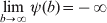$\mathop {\lim }\limits_{b \to \infty } \psi \lpar b\rpar \equals \minus \infty $. Hence the non-linear equation

(19)$$\lpar \chi \minus \lambda \rpar b \plus {\rm \gamma }b^{\setnum{1} \minus \setnum{1}\sol {\rm \gamma }} \plus \xi \lambda \equals 0$$

has a unique solution that is denoted by b* and it can be shown that the verification theorem holds (Pham, Reference Pham2009). Finally we note that for ξ=0 (no bequest motive) b*=(γ/(λ−χ))^γ. Thus we have the following result that is due to Merton (Reference Merton1969).

Conclusion 1.If the conditions in Proposition 1 are satisfied, the conditions 0<γ<1 and χ<λ hold and the lifetime distribution is exponential with parameter λ then

(20)$${\rm \pi }{\ast } \equals {{\mu \minus r} \over {\gamma \sigma ^{\setnum{2}} }}\quad {\rm and}\quad c{\ast } \equals w \cdot \lpar b{\ast } \rpar ^{ \minus \setnum{1}\sol {\rm \gamma }} $$

is an optimal control of the retiree's maximization problem (16). In the maximization problem without bequest motive, i.e., ξ=0, the optimal control c* is given by

(21)$$c{\ast } \equals w \cdot {{\lambda \minus \chi } \over \gamma }.$$

If the lifetime T follows an exponential distribution, the optimal share π* of the risky asset does neither depend on wealth nor on time. The independence of wealth is not surprising because by assumption we look at a retiree with constant relative risk aversion. Only if the return of the riskless asset, the volatility of the risky asset, or the relative risk aversion decrease, or the expected return of the risky asset increases the investment in the risky asset becomes more attractive compared with the riskless investment. The retiree raises the share of the risky assets. His portfolio selection is thus independent of consumption (Merton, Reference Merton1969). The optimal consumption strategy is constant and also consistent with Merton (Reference Merton1969) .

As for an exponential lifetime distribution the differential equation (18) reduces to the non-linear equation (19), in contrast with the case of a general lifetime distribution, there is no problem of finding an appropriate initial value a ₀ for which the solution of (18) satisfies the conditions of the verification theorem and is an optimal control therefore. Later in Section 6 we circumvent the verification theorem in the general case by maximizing the total discounted utility as a function of a ₀.

6 Optimal control

The structure of c* and π* in (20) is the motivation to study the class of all control strategies for which consumption is proportional to wealth, where the corresponding factor may depend on time t, and the portfolio function π_s does not depend on wealth. Set

(22)$${\cal L} \equals \lcub \lpar c\comma \pi \rpar \colon c_{t} \lpar w\rpar \equals \rho \lpar t\rpar w\comma \pi _{t} \lpar w\rpar \equals \kappa \lpar t\rpar \rcub \comma $$

where ρ is non-negative and both κ and ρ are continuous. Note that by the construction of the capital market model the two functions c_t and π_t act, with respect to wealth, in a different way. Whereas by construction π_t is already a proportion of wealth (π_tW_t is to be invested in the risky asset) the consumption c_t(W_t) is any function of W_t. But now ρ(t) is the proportion of W_t that can be consumed so that both ρ and κ play the role of proportions.

By (5) the wealth process is given by

(23)$$W_{t} \equals w_{\setnum{0}} \plus \int_{\setnum{0}}^{t} {W_{s} A\lpar s\rpar ds \plus } \int_{\setnum{0}}^{t} {W_{s} D\lpar s\rpar dB_{s} \comma } $$

With

(24)$$A\lpar s\rpar \equals \kappa \lpar s\rpar \mu \plus \lpar 1 \minus \kappa \lpar s\rpar \rpar r \minus \rho \lpar s\rpar \quad {\rm and}\quad D\lpar s\rpar \equals \kappa \lpar s\rpar \sigma .$$

Ito's formulaFootnote ⁸ shows that the unique solution is given by

(25)$$W_{t} \equals w_{\setnum{0}} \exp \left\{ {\int_{\setnum{0}}^{t} {A\lpar s\rpar ds} \minus {1 \over 2}\int_{\setnum{0}}^{t} {D^{\setnum{2}} \lpar s\rpar ds \plus } \int_{\setnum{0}}^{t} {D\lpar s\rpar dB_{s} } } \right\}.$$

Using the modified utility function ${\cal U}_{\gamma } $ in (12) the total discounted utility is defined by

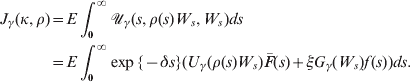(26)$$\eqalign{ J_{\gamma } \lpar \kappa \comma \rho \rpar \equals \tab E\int_{\setnum{0}}^{\infty } {{\cal U}_{\gamma } \lpar s\comma \rho \lpar s\rpar W_{s} \comma W_{s} \rpar } ds \cr \equals \tab E\int_{\setnum{0}}^{\infty } {\exp \lcub \minus \delta s\rcub \lpar U_{\gamma } \lpar \rho \lpar s\rpar W_{s} \rpar \bar{F}\lpar s\rpar \plus \xi G_{\gamma } \lpar W_{s} \rpar f\hskip 1\lpar s\rpar \rpar ds.} \cr} $$

Confining to 0<γ<1 we have

$${\cal U}_{\gamma } \lpar t\comma c\comma w\rpar \equals \exp \lcub \minus \delta t\rcub {1 \over {1 \minus \gamma }}c^{\setnum{1} \minus \gamma } \bar{F}\lpar t\rpar \plus \xi \exp \lcub \minus \delta t\rcub {1 \over {1 \minus \gamma }}\comma w^{\setnum{1} \minus \gamma } f\hskip 1\lpar t\rpar $$

so that we may write the total discounted utility as

$$\eqalign{ J_{\gamma } \lpar \kappa \comma {\kern 1pt} \rho \rpar \equals \tab E\int_{\setnum{0}}^{\infty } {{1 \over {1 \minus \gamma }}} \exp \lcub \minus \delta t\rcub \lpar \bar{F}\lpar t\rpar \lpar \rho \lpar t\rpar W_{t} \rpar ^{\setnum{1} \minus \gamma } \plus \xi f\hskip 1\lpar t\rpar W_{t}^{\setnum{1} \minus \gamma } \rpar dt \cr \equals \tab \int_{\setnum{0}}^{\infty } {\lpar EW_{t}^{\setnum{1} \minus \gamma } \rpar } {1 \over {1 \minus \gamma }}\exp \lcub \minus \delta t\rcub \lpar \bar {F}\lpar t\rpar \lpar \rho ^{\setnum{1} \minus \gamma } \lpar t\rpar \plus \xi f\hskip 1\lpar t\rpar \rpar dt. \cr} $$

In order to evaluate EW_t ^1−γ we use (33) in the Appendix where A and D are specified by (24). This gives

$$\eqalign{ J_{\gamma } \lpar \kappa \comma {\kern 1pt} \rho \rpar \equals \tab {{w_{\setnum{0}}^{\setnum{1} \minus \gamma } } \over {1 \minus \gamma }}\int_{\setnum{0}}^{\infty } {\exp \lcub \minus \delta t\rcub } \lpar \bar{F}\lpar t\rpar \rho ^{\setnum{1} \minus \gamma } \lpar t\rpar \plus \xi f\hskip 1\lpar t\rpar \rpar \cr \tab \times \exp \left\{ {\lpar 1 \minus \gamma \rpar \int_{\setnum{0}}^{t} {\lpar 1 \minus \kappa \lpar s\rpar \rpar r \plus \kappa \lpar s\rpar \mu \minus \rho \lpar s\rpar } \minus {{\gamma \sigma ^{\setnum{2}} \kappa \lpar s\rpar ^{\setnum{2}} } \over 2}ds} \right\}dt. \cr} $$

Our aim is to maximize the functional J _γ(κ, ρ). As the exponent is quadratic in κ and linear in ρ, we may carry out the maximization with respect to κ in a first step. The function

$$\kappa \; \mapsto \; \lpar 1 \minus \kappa \rpar r \plus \kappa \mu \minus \rho \lpar s\rpar \minus {{{\rm \gamma }\sigma ^{\setnum{2}} \kappa ^{\setnum{2}} } \over 2}$$

attains the maximum at

(27)$$\kappa {\ast } \equals {{\mu \minus r} \over {\gamma \sigma ^{\setnum{2}} }}.$$

This means that the optimal proportion of wealth that is invested in risky assets is again independent of time. Instead it depends on the difference between the expected return of the risky asset and the return of the riskless asset as well as on the volatility of the risky asset and the retiree's risk aversion. Thus we have shown that the result concerning the optimal portfolio function (see π* in (20)) still holds if we look at a lifetime distribution with logistic (instead of constant) mortality rates. The independence of lifetime and asset returns is one reason for this result. The other ingredient that contributes to this result is the product structure of the utility function. Both facts allow solving the HJB equation by a separation of strategies that finally leads to Merton's strategy.

Since κ* provides the maximum, it holds

$$\lpar 1 \minus \kappa \rpar r \plus \kappa \mu \minus \rho \lpar s\rpar \minus {{{\rm \gamma }\sigma ^{\setnum{2}} \kappa ^{\setnum{2}} } \over 2}\leqslant r \minus \rho \lpar s\rpar \plus {{\lpar \mu \minus r\rpar ^{\setnum{2}} } \over {2{\rm \gamma }\sigma ^{\setnum{2}} }}$$

so that for every κ

(28)$$J_{\gamma } \lpar \kappa \comma {\kern 1pt} \rho \rpar \le J_{\gamma } \lpar \kappa {\ast } \comma \rho \rpar \equals {{w_{\setnum{0}}^{\setnum{1} \minus \gamma } } \over {1 \minus \gamma }}\int_{\setnum{0}}^{\infty } {\rmGamma \lpar t\rpar \exp \left\{ {\lpar 1 \minus \gamma \rpar \left( {Rt \minus \int_{\setnum{0}}^{t} {\rho \lpar s\rpar ds} } \right)} \right\}dt\comma } $$

where

$$\rmGamma \lpar t\rpar \equals \exp \lcub \minus \delta t\rcub \lpar \bar{F}\lpar t\rpar \rho ^{\setnum{1} \minus \gamma } \lpar t\rpar \plus \xi\hskip1 f\hskip1\lpar t\rpar \rpar \quad {\rm and}\quad R \equals r \plus \lpar \mu \minus r\rpar ^{\setnum{2}} \sol \lpar 2\gamma \sigma ^{\setnum{2}} \rpar .$$

We know from Proposition 1 that $c{\ast } \equals w \cdot \lpar \bar{F}\sol a\rpar ^{\setnum{1}\sol \gamma } $ is the consumption that comes out from the solution of HJB equation, where a satisfies the ordinary differential equation

(29)$$a \prime \lpar t\rpar \plus a\lpar t\rpar \chi \plus \gamma a^{\setnum{1} \minus \setnum{1}\sol {\rm \gamma }} \lpar t\rpar \bar{F}^{\,\setnum{1}\sol {\rm \gamma }} \lpar t\rpar \plus \xi f\hskip 1\lpar t\rpar \equals 0.$$

If the bequest motive is absent, then the differential equation becomes

$$a\prime \lpar t\rpar \plus a\lpar t\rpar \chi \plus \gamma a^{\setnum{1} \minus \setnum{1}\sol {\rm \gamma }} \lpar t\rpar \bar{F}^{\,\setnum{1}\sol {\rm \gamma }} \lpar t\rpar \equals 0\comma $$

which is a Bernoulli type differential equation that, by the substitution

$$k\lpar t\rpar \equals a^{\setnum{1}\sol \gamma } \lpar t\rpar \comma $$

is transformed into

$$k\prime \lpar t\rpar \plus {\chi \over {\rm \gamma }}k\lpar t\rpar \plus \bar{F}^{\,\setnum{1}\sol {\rm \gamma }} \lpar t\rpar \equals 0.$$

The solution of the initial value problem is given by

$$k\lpar t\rpar \equals \exp \left\{ { \minus {\chi \over \gamma }t} \right\}\left( {k_{\setnum{0}} \minus \int_{\setnum{0}}^{t} {\bar{F}^{\,\setnum{1}\sol \gamma } \lpar s\rpar \exp \left\{ { \minus {\chi \over \gamma }s} \right\}ds} } \right).$$

We have already pointed out that to solve the control problem one has to check the conditions of the verification theorem for a solution of the HJB equation and that this is impossible unless the solution is explicitly known. To circumvent these difficulties we use another approach.

Denote by a(t, a ₀, ξ) the solution of (29) that satisfies the initial condition a(0, a ₀, ξ)=a ₀. Let furthermore be

$$\rho \lpar t\comma a_{\setnum{0}} \comma \xi \rpar \equals \left( {{{\bar{F}\lpar t\rpar } \over {a\lpar t\comma a_{\setnum{0}} \comma \xi \rpar }}} \right)^{\setnum{1}\sol \gamma } .$$

Instead of verifying the condition (17) we directly investigate the total discounted utility. Within the family a(t, a ₀, ξ) we find the optimal solution that solves the control problem by maximizing J _γ(κ*, ρ(⋅, a ₀, ξ)) as function of a ₀. Thus we have the following result.

Proposition 2Suppose that the assumptions of Proposition 1 are fulfilled and that a(t, a ₀, ξ) is the solution of(15) with a(0, a ₀, ξ)=a ₀. If a*₀is a maximum point of the function $a_{\setnum{0}} \mapsto J_{\gamma } \lpar \kappa {\ast } \comma \rho \lpar \cdot \comma a_{\setnum{0}} \comma \xi \rpar \rpar $, then c* and π* in(14) are solutions of the control problem(16) provided that a(t, a*₀, ξ) is a solution of the ordinary differential equation(15) with initial value a*₀.

The meaning of the above result consists in the fact that for any given lifetime distribution, the right hand term in (28) is an explicit expression that can be maximized as a function of a ₀, at least numerically. This is a new way to circumvent the difficulties with the verification theorem.

7 Application

In this section we apply Proposition 2 in order to find the optimal consumption for retirees in Germany. To this end we have to choose an appropriate lifetime distribution. We use the logistic model from Section 3 and apply the estimated parameters in (2). For fixed parameter values r=δ=0.02, μ=0.05, σ=0.2 (Stabile, Reference Stabile2006; Babbel and Merril, Reference Babbel and Merril2007), and γ=0.7, a numerical evaluation of the appearing integrals leads for different values of ξ to the following optimal consumption strategies c_t*(w)=w⋅ρ(t, a*₀, ξ). Referring to Cocco et al. (Reference Cocco, Gomes and Maenhout2005) we let ξ vary from 0 to 4. The curves ρ(t, a*₀, ξ) for ξ=0, ξ=0.5, ξ=1, ξ=2 and ξ=4 are collected in Figure 2.

Figure 2.

(colour online) Optimal consumption curves for different weights of the bequest motive (0; 0.5; 1; 2; 4).

The optimal consumption curves are remarkable in several aspects. While the optimal consumption ratio is independent of time if we assume an exponential distribution of lifetime with constant mortality rate (see Conclusion 1), it changes over time if we use the logistic model. In the case without bequest motive the optimal consumption ratio increases over time until about 92 (=65+27) years. Moreover, it shows an increasing growth until about 90 years, afterwards the positive slope of the curve decreases. After about 92 years the optimal consumption ratio sharply decreases down to zero. The rise and fall of the optimal consumption ratio are smoothed by the extent of the bequest motive.

The story behind the non-monotonous run of the curves might be the following: Since the mortality rate exponentially increases during the early years of retirement, a retiree raises his consumption rates during this period. At about 90 years, when he is still alive, he notices that he now faces the risk of longevity because from now on the increase in the mortality rate will continuously decline over the remaining years. Thus he starts not to raise his consumption ratio that much anymore and finally he even decreases it.

The magnitudes of the ups and downs of the consumption ratio are smoothed by the intensity of the bequest motive. Not surprisingly, this motive basically has a negative impact on the optimal consumption ratio. A retiree who wants to have a positive property W_T at his stochastic date of death T chooses a relatively low consumption ratio (and does not increase it that much) whereas for a retiree without any intention to leave some money to his heirs a higher, more rapidly increasing (and later decreasing) consumption ratio is optimal.