1. Introduction
Emerging markets and developing economies (EMDEs) have been accumulating a tremendous amount of foreign exchange (FX) reserves since the late 1990s. The dramatic increase in FX reserve holdings has prompted an active debate on optimal reserve management (International Monetary Fund, 2011, 2013). What is the optimal policy for FX reserve management? This is a challenging question, especially for EMDEs that struggle with credibility problems in policymaking.
This paper studies optimal FX reserve management without commitment. The paper builds on a stylized linear-quadratic small-open economy framework à la Ghosh et al. (Reference Ghosh, Ostry and Chamon2016) and Basu et al. (Reference Basu, Ghosh, Ostry and Winant2018). The model has three key ingredients: (i) fear of floating, (ii) forward-looking exchange rates, and (iii) the cost of reserve management. First, the fear of floating is widespread in EMDEs (Calvo and Reinhart, Reference Calvo and Reinhart2002), which motivates exchange rate management through the accumulation of FX reserves. The model incorporates fear of floating as a convex welfare cost, following Bianchi and Lorenzoni (Reference Bianchi and Lorenzoni2022). Second, in the model, exchange rates are determined through the expectation channel, as in Basu et al. (Reference Basu, Ghosh, Ostry and Winant2018). Since the exchange rate is forward-looking, both the current policy stance and the future policies influence the exchange rate today.Footnote 1 Last, the cost of reserve management is incorporated as a convex welfare cost. The reserve management cost is an important consideration for EMDEs that includes the foregone opportunity cost of investment and the quasi-fiscal sterilization cost.
In this framework, I first derive two optimal policies: the Ramsey policy and the Markov-Perfect policy. These serve as benchmark policies for a government with and without commitment. The two policies differ in how they address the trade-offs between the fear of floating and the cost of reserve management. I show that the Ramsey policy yields higher welfare in equilibrium than the Markov-Perfect policy. This result highlights the importance of credibility in reserve management. Without commitment, however, the government has an incentive to deviate from the Ramsey policy. In other words, the Ramsey policy is time-inconsistent. I propose a simple policy to achieve the Ramsey outcome without commitment. Specifically, the suggested sustainable plan incentivizes subsequent governments to follow the prescribed policy path, ensuring the Ramsey outcome in equilibrium.
This paper is related to the literature on optimal FX reserve management. Jeanne and Rancière (Reference Jeanne and Rancière2011) provide a measure of the optimal FX reserves in the economies susceptible to sudden stops. More recently, Arce et al. (Reference Arce, Bengui and Bianchi2019) examine the macroprudential role of reserve accumulation in achieving constrained efficiency. Céspedes and Chang (Reference Céspedes and Chang2024) emphasize the interaction between ex-ante reserve accumulation and ex-post unconventional monetary policies. Despite its importance, the issue of commitment in reserve management has been less explored in the literature. Basu et al. (Reference Basu, Ghosh, Ostry and Winant2018) is one of the few studies that highlight credibility issues. While Basu et al. (Reference Basu, Ghosh, Ostry and Winant2018) focus on capital outflow episodes, the present study examines the time inconsistency that arises in normal times due to the cost of reserve management. In addition, this study provides a sustainable plan to implement the Ramsey outcome without commitment, overcoming the credibility problem.
This paper also relates to the literature on the time inconsistency of government policies (Calvo, Reference Calvo1978; Kydland and Prescott, Reference Kydland and Prescott1980; Barro and Gordon, Reference Barro and Gordon1983). Stokey (Reference Stokey1989, Reference Stokey1991) and Chari and Kehoe (Reference Chari and Kehoe1990) propose the notion of sustainable plan for credible government policy.Footnote 2 Seminal works along this line includes Chang (Reference Chang1998) and Phelan and Stacchetti (Reference Phelan and Stacchetti2001), which provide complete characterizations of sustainable plans for monetary and fiscal policies using the technique developed by Abreu et al. (Reference Abreu, Pearce and Stacchetti1990). The present study does not attempt to characterize the set of sustainable plans. Instead, it proposes a simple, sustainable plan in the context of FX reserve management, highlighting the issue of credibility.
The paper is organized as follows. Section 2 describes the model. Section 3 studies the Ramsey and the Markov-Perfect policies. Section 4 provides a sustainable plan. Section 5 concludes.
2. Model
Time is discrete and denoted by
 $t\in \{0,\ldots ,\infty \}$
. Consider a small-open and perfect-foresight economy in which the equilibrium is characterized by three linear equations: capital flow, current account, and the balance of payment.Footnote
3
The capital flow is determined by
 \begin{align*} \Delta k_t = \alpha ( r_t - (r^*_t + e_{t+1}-e_t)) \end{align*}
where
 $\Delta k_t$
is the change in capital flows,
 $r_t$
and
 $r_t^*$
are the real interest rates in the domestic and the foreign economies,
 $e_t$
is the real exchange rate, and
 $\alpha \gt 0$
.Footnote
4
This equation is a variant of the uncovered interest rate parity (UIP) condition describing private agents’ behavior of absorbing excess returns in the financial market.Footnote
5
The foreign capital flows into the domestic economy (i.e.,
 $\Delta k_t \gt 0$
), whenever there is an excess return from holding domestic bonds after taking into account expected exchange rate adjustments (i.e.,
 $ r_t \gt r^*_t + e_{t+1}-e_t$
). The foreign capital flows out of the domestic economy whenever the opposite holds.
Assume that the real interest rates are the same in the domestic and the foreign economies
 $r_t=r^*_t$
, abstracting from policy rate considerations. The equation is then reduced to
 \begin{align} \Delta k_t = \alpha (e_t-{e_{t+1}}) \end{align}
which shows that capital inflows
 $\Delta k_t \gt 0$
(capital outflows
 $\Delta k_t \lt 0$
) are associated with expected currency appreciations
 $e_t\gt e_{t+1}$
(expected currency depreciations
 $e_t\lt e_{t+1}$
).
The current account is normalized to be balanced at
 $e_t=0$
, in particular,
 \begin{align} ca_t = \gamma e_t \end{align}
with
 $\gamma \gt 0$
, indicating that the current account surplus is associated with exchange rate depreciation.
Finally, from the balance of payment identity, the current account is equal to the change in the net foreign assets held by the economy
 \begin{align} ca_t = \Delta R_t - \Delta k_t \end{align}
where
 $\Delta R_t$
is the change in the stock of FX reserves.
Definition 1.
A perfect-foresight equilibrium is composed of sequences of capital flow, exchange rate, and current account
 $\{k_t,e_t,ca_t\}_{t=0}^{\infty }$
satisfying(
1
), (
2
), and(
3
), given the stock of FX reserves
 $\{R_t\}_{t=0}^{\infty }$
chosen by the government, and the initial conditions
 $k_{-1},R_{-1}$
.
Given
 $\{R_t\}_{t=0}^{\infty }$
chosen by the government and initial conditions
 $k_{-1}$
and
 $R_{-1}$
, the equilibrium conditions are summarized as the following system of equations.
 \begin{align}& e_t = \frac {\alpha }{\alpha +\gamma }e_{t+1} + \frac {1}{\alpha +\gamma } \Delta R_t \\[-10pt]\nonumber \end{align}
 \begin{align}&\qquad\qquad ca_t = \gamma e_t \\[-10pt]\nonumber\end{align}
 \begin{align}&\qquad \Delta k_t = \Delta R_t-\gamma e_t \end{align}
Equation (4) shows that the exchange rate is forward-looking as it responds to the expected future exchange rate. It also shows that the exchange rate depreciates when reserves are accumulated, that is,
 $\Delta R_t\gt 0$
. This implies that the reserve management policy affects not only the exchange rate in the current period but also the exchange rates in all previous periods through expectations.
Suppose that the per-period welfare of the economy is in quadratic form
 \begin{align} -U(e_t,\Delta R_t) \equiv -\frac {(e_t-\bar {e})^2}{2} - \frac {\theta }{2}(\Delta R_t)^2 \end{align}
The first term, called the fear of floating, is the convex welfare cost that incurs whenever the exchange rate is away from the bliss level
 $\bar {e}\gt 0$
. The second term is the convex cost of reserve management.
How should the government optimally manage reserves? The welfare function in equation (7) illustrates the trade-offs involved in reserve management. On the one hand, due to the fear of floating, the government aims to achieve the optimal exchange rate level by adjusting reserve stocks. On the other hand, due to the cost of reserve management, the government seeks to minimize changes in reserve holdings. Let
 $f_t\equiv \Delta R_t$
be the variable for reserve management, that is, positive (negative)
 $f_t$
indicates reserve accumulation (decumulation). The government policy for reserve management is denoted by a sequence
 $\vec {f}=\{f_t\}_{t=0}^\infty$
.
Definition 2.
The government policy for reserve management is
 $\vec {f}$
and the associated equilibrium outcome can be backed out from(
4
)–(
6
).
The next section studies two benchmark optimal policies for reserve management with and without commitment. With commitment, the government is able to follow Ramsey policy achieving the first-best Ramsey outcome in equilibrium. Markov-Perfect policy is a policy for the government without commitment.
3. Optimal policies for reserve management
3.1 Ramsey policy
Consider the Ramsey planning problem that maximizes the discount sum of the per-period welfare (7)
 \begin{align*} \max _{\vec {e},\vec {f}} \sum _{t=0}^\infty \beta ^t\left \{-U(e_t,f_t)\right \} \end{align*}
subject to the equilibrium conditions (4) – (6).
The Ramsey problem in recursive form is composed of two subproblems. In the second subproblem, the Ramsey planner solves
 $\max _{e_0} J(e_0)$
, where the value function
 $J$
solves the first subproblem of the Bellman equation
 \begin{align} J(e) = \max _{f,e'} -U(e,f) + \beta J(e')\ \ \ \text{subject to}\ \ \ e = \frac {\alpha }{\alpha +\gamma }e' + \frac {1}{\alpha +\gamma } f \end{align}
The solution to this problem is called the Ramsey plan denoted by
 $\{\vec {e}^R,\vec {f}^R\}$
, where
 $\vec {e}^R=\{e^R_t\}_{t=0}^\infty$
and
 $\vec {f}^R=\{f^R_t\}_{t=0}^\infty$
. In particular,
 $\vec {f}^R$
is the Ramsey policy on reserve management.
Assumption 1.
Assume that
 $\beta = \alpha / (\alpha + \gamma )$
, that is, the discount factor of the economy is consistent with that one of the Ramsey planner.
Proposition 1.
Under Assumption
1
, the Ramsey plan is
 $\{\vec {e}^R,\vec {f}^R\}$
s.t.
 \begin{align*} e_{t+1}^R &= \omega ^R e^R_{t}+\left (1-\omega ^R\right )\bar {e} \\ f_t^R &= (\alpha + \gamma )\left (1-\omega ^R \beta \right ) (e_t -\bar {e}) + \gamma \bar {e} \end{align*}
with
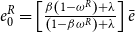 $e^R_0 = \left [\frac {\beta \left (1-\omega ^R\right ) + \lambda }{\left (1-\beta \omega ^R\right )+\lambda } \right ]\bar {e}$
, where
 $\omega ^R = \frac {1}{2\beta }\left (1+\beta + \lambda - \sqrt {(1+\beta + \lambda )^2 - 4\beta }\right )$
and
 $\lambda = 1/ (\theta (\alpha + \gamma )^2)$
.
Proof. See Appendix A.
Note that the initial exchange rate
 $e_0^R$
is lower than the bliss point of exchange rate
 $\bar {e}$
, that is, the currency is appreciated than the desired level to begin with. Since
 $f_t^R\gt 0$
and
 $e_{t+1}$
is the weighted average of
 $e_{t}$
and
 $\bar {e}$
, FX reserves are accumulated and the currency depreciates as the economy converges to the steady state. Once the economy reaches the steady state, exchange rate stays at
 $\bar {e}$
supported by policy
 $f_t^R= \gamma \bar {e}$
.
Suppose that
 $\omega ^R$
increases. In this case, which may arise when the cost of reserve management goes up (i.e., higher
 $\theta$
), the appreciation rate is relatively small and the reserve policy becomes less active.Footnote
6
3.2 Markov-Perfect policy
The Markov-Perfect policy depends only on the payoff-relevant current state. This means that Markov-Perfect policy on reserve management
 $\vec {f}^{MP}=\{f^{MP}_t\}^{\infty }_{t=0}$
is constant in all periods, that is,
 $f_t^{MP} = f^{MP}$
for some constant
 $f^{MP}$
.
Given
 $f_{t+j+1}= f^{MP}$
for
 $j\geq 0$
, the Markov-Perfect policy solves
 \begin{align} \max _{\vec {f}} \sum _{t=0}^\infty \beta ^t\left \{-U(e_t,f_t)\right \} \end{align}
subject to the equilibrium conditions (4) – (6).
Proposition 2.
The Markov-Perfect policy is
 $\{\vec {f}^{MP}\}$
and the associated equilibrium exchange rate is
 $\{\vec {e}^{MP}\}$
s.t.
 $e_{t}^{MP} = \omega ^{MP}\bar {e}$
and
 $f_{t}^{MP} = \gamma \omega ^{MP}\bar {e}$
where
 $\omega ^{MP} = 1/(1+\theta \gamma (\alpha + \gamma ))$
.
Proof. See Appendix C.
3.3 Comparison between Ramsey policy and Markov-Perfect policy
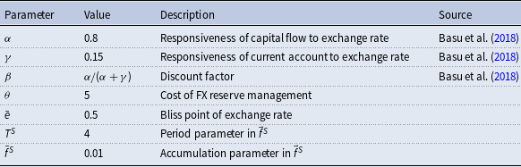
This section presents numerical results for the Ramsey and the Markov-Perfect policies. The parameter values are summarized in Table 1. I set
 $\theta$
to 5 and
 $\bar {e}$
to 0.5 in order to clearly illustrate welfare trade-offs. I normalize the initial values of
 $k_{-1}$
and
 $R_{-1}$
to zero.
Parameter values

Equilibrium time paths under Ramsey and Markov-Perfect policies.

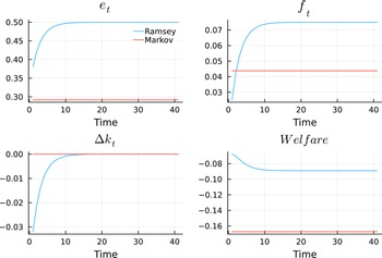
Figure 1 describes the equilibrium outcomes under the Ramsey policy and the Markov-Perfect policy. As noted, there is a trade-off between fear of floating and reserve management cost as reflected in the welfare (7). Under the Markov-Perfect policy, reserves are accumulated at a constant rate. This means that the government sets the same accumulation rate in each period to balance out the trade-offs. Accordingly, the exchange rate is constant over time, resulting in no changes in capital flows, as shown in the figure. In contrast, under the Ramsey policy, the time-consistent government resolves the trade-offs intertemporally through the expectation channel of exchange rate. Specifically, the government gradually increases the pace of reserve accumulation in the first 10 periods. In this acceleration phase, the exchange rate depreciates until it reaches the bliss point. The currency depreciation is not solely due to the contemporaneous reserve accumulation. The promised future accumulation also affects the current exchange rates through the expectation channel. The Ramsey government credibly makes a promise about reserve accumulations in the future, letting the current exchange rate depreciate closer to the bliss level. After reaching the bliss level
 $\bar {e}$
, the Ramsey policy keeps a constant rate of accumulation
 $\gamma \bar {e}$
to support the exchange rate.
Under the Markov-Perfect policy, the level of capital stays at the initial value, since there is no change in exchange rates. Under the Ramsey policy, the economy experiences capital outflows in the first 10 periods, resulting in a lower level of capital stock. This is again due to the expected future exchange rate depreciations. Since the government gradually increases the pace of reserve accumulation under the Ramsey policy, the reserve stock is lower in the first three periods compared to the one under the Markov-Perfect policy. But, eventually, more reserves are accumulated under the Ramsey policy.
The Ramsey policy achieves higher welfare than the Markov-Perfect policy. The figure shows that the overall welfare evaluated at time 0 is greater under the Ramsey policy (−0.06) than the Markov-Perfect policy (−0.167). The figure also illustrates that the welfare level is higher under the Ramsey policy along the time path. The overall welfare difference between the two policies is due to the availability of commitment device. The economy is better off if the government is able to make a credible promise about its reserve management.
Result 1.
The Ramsey policy
 $\vec {f}^{R}$
brings greater welfare than the Markov-Policy
 $\vec {f}^{MP}$
.
The above results leave us with several questions. What is the best equilibrium outcome for the government without commitment? Is it possible to achieve higher welfare than the one under Markov-Perfect policy? If so, how? The next section provides a way to implement the Ramsey outcome for the government without commitment.
4. Sustainable plan for reserve accumulation
Without commitment, it is difficult for the government to implement the Ramsey policy. This is because Ramsey policy is not time-consistent, that is, the subsequent governments face deviation incentives from the policy. In particular, there is a temporary gain from avoiding the cost of reserve management. To see this, consider a government that sets
 $f_\tau =0$
in period
 $\tau$
and then switch to the Ramsey policy in the following period, that is,
 $f_\tau =0$
and
 $f_{\tau +1}=f^R_{\tau +1}$
. Note that
 \begin{align*} -U\left(e^R_{\tau },0\right) + \beta J\left(e^R_{\tau +1}\right) &\geq -U\left(e^R_\tau ,e^R_\tau \right) + \beta J\left(e^R_{\tau +1}\right) \\ -U\left(e^R_\tau ,0\right) &\geq -U\left(e^R_\tau ,f^R_\tau \right) \end{align*}
since
 $-\frac {\theta }{2} (f^R_\tau )^2 \leq 0$
.
Hence, to achieve the Ramsey outcome, one must come up with a contingency plan that specifies not only the policy implemented along the equilibrium path but also the punishment that deters incentives to deviate. Such a plan is called a sustainable plan.
Definition 3.
A plan
 $\vec {f}$
is sustainable if it prevents any deviations from the plan.
One way to construct the punishment scheme for a sustainable plan is to use a self-enforcing plan defined below.
Definition 4.
A plan
 $\vec {f}$
is self-enforcing if it deters any deviations by restarting the plan in period
 $j+1$
when there is a deviation in period
 $j\geq 0$
.
Equilibrium time path under the self-enforcing plan.

Consider a plan
 $\vec {f}^{S}$
that sets
 $f_t^S$
at a low constant rate
 $\bar {f}^S$
for the first
 $T^S$
periods and then switches to Ramsey policy
 $\vec {f}^R$
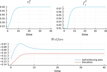
afterwards. The plan restarts itself if there is a deviation in any period. Notice that this plan is self-enforcing and deters any deviations with
 $T^S=4$
and
 $\bar {f}^S=0.01$
as shown in Figure 2. Under
 $\vec {f}^{S}$
, reserves are accumulated at a constant low rate
 $\bar {f}^S$
for the first four periods. For period
 $t \geq T^S+1$
, the government switches to
 $\vec {f}^R$
. Compared to the Ramsey policy, the economy attainslower level of welfare (−0.12) evaluated at time 0. But importantly, unlike the Ramsey policy, this plan does not suffer from the time-inconsistency issue. The figure shows that the government cannot find any profitable deviations from the plan. This means the low rates of
 $\bar {f}^S$
in the first
 $T^S$
periods are strong punishments to the government. Thus, the plan
 $\vec {f}^{S}$
successfully prevents deviation incentives by rewarding the government with high welfare associated with the Ramsey outcome only if it endures low welfare in the first
 $T^S$
periods.
Result 2.
The plan
 $\vec {f}^{S}$
with
 $T^S = 4, \bar {f}^S = 0.01$
is self-enforcing.
Now consider a sustainable plan that delivers the Ramsey outcome in equilibrium constructed using the self-enforcing plan
 $\vec {f}^{S}$
as a punishment. Specifically, this plan, denoted by
 $\vec {f}^{RS}$
, follows the Ramsey policy
 $\vec {f}^R$
until there is any deviation. When there is a deviation, the plan switches to
 $\vec {f}^{S}$
permanently. Specifically, the plan
 $\vec {f}^{RS}$
is defined as
 $\{f_t^{RS}\}^{\infty }_{t=0}$
s.t.
 \begin{align*} f_t^{RS} = \begin{cases} f_t^R & \text{if } t\lt \tau \\ f_t^S & \text{if } t\geq \tau \end{cases} \end{align*}
for any period
 $\tau$
where there is a deviation.
As long as the permanent punishment of
 $\vec {f}^{S}$
is sufficiently strong,
 $\vec {f}^{RS}$
is sustainable. In other words,
 $\vec {f}^{RS}$
is sustainable if
 \begin{align} v_j^{R} \geq -U\left(e_j^R,0\right) + \beta v_0^{S} \end{align}
for any period
 $j\geq 0$
. The left-hand side of (10) is the welfare associated with the Ramsey outcome in period
 $j$
that the government can achieve by following
 $\vec {f}^{RS}$
 \begin{align*} v_j^R\equiv \sum _{t=j}^\infty \beta ^t\left \{-U\left(e_t^R,f_t^R\right)\right \} \end{align*}
The right-hand side of (10) is the sum of the temporary gain from deviating to
 $f_t=0$
and the welfare from
 $\vec {f}^{S}$
that the government receives after the deviation
 \begin{align*} v_0^S\equiv \sum _{t=0}^\infty \beta ^t\left \{-U\left(e_t^S,f_t^S\right)\right \} \end{align*}
Welfare comparison: the sustainable plan and deviations from it.

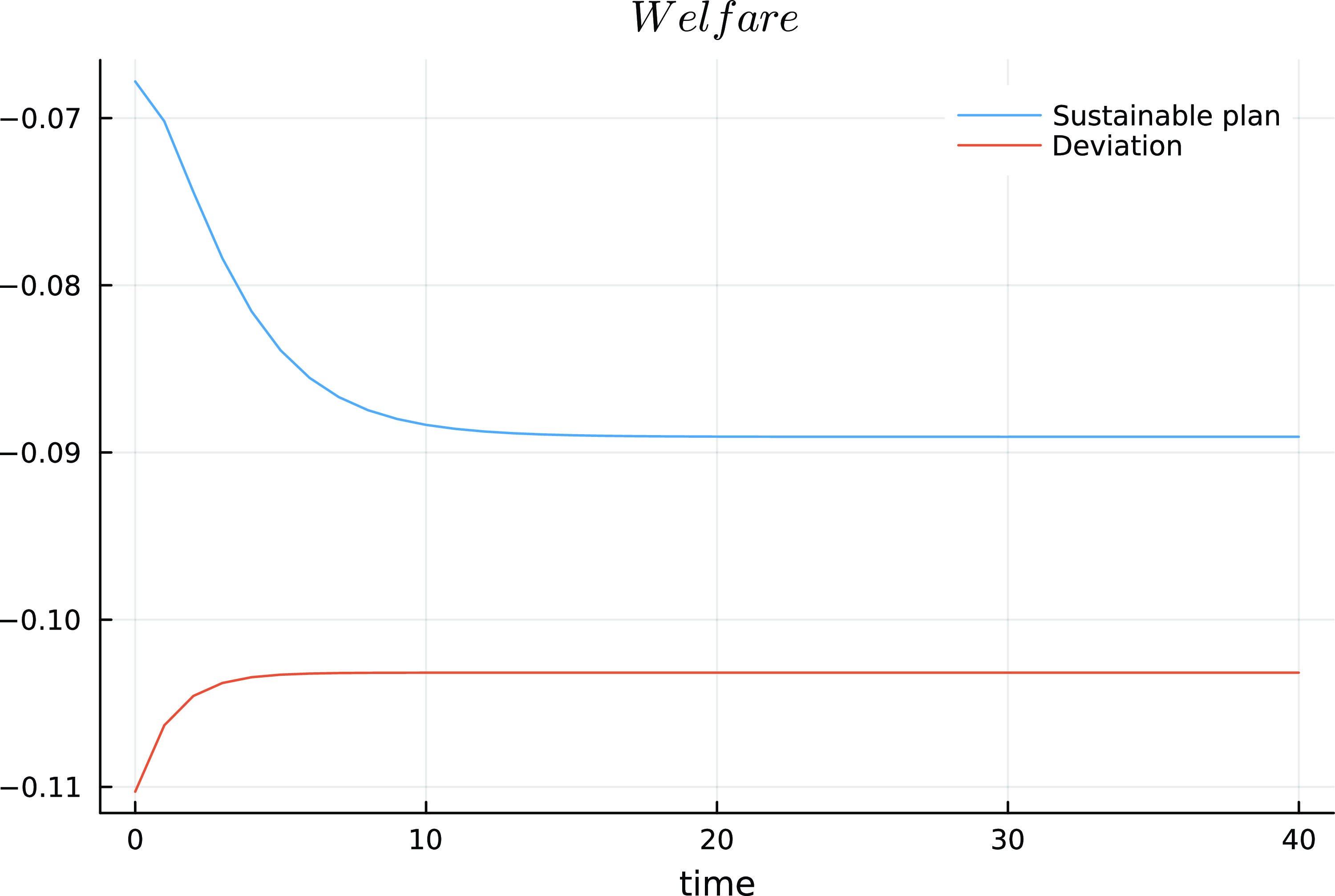
Figure 3 demonstrates that the plan
 $\vec {f}^{RS}$
is indeed sustainable under the given parameterization. The welfare from
 $\vec {f}^{RS}$
is the same as the one from
 $\vec {f}^{R}$
shown in Figure 1. This is because
 $\vec {f}^{RS}$
achieves the Ramsey outcome on the equilibrium path without any deviations. Along the time path, the welfare from
 $\vec {f}^{RS}$
is greater than the one from deviations. The permanent punishment
 $\vec {f}^S$
is so strong that the government does not have incentives for deviation. This shows that, by following plan
 $\vec {f}^{RS}$
, the government without commitment achieves the Ramsey outcome in equilibrium.
Result 3.
The plan
 $\vec {f}^{RS}$
is sustainable. Following this plan, the government achieves the Ramsey outcome in equilibrium without commitment.
5. Conclusion
The central banks in EMDEs have been using FX reserves as an important policy tool. Nevertheless, the optimal management of FX reserves remains a topic of debate. Managing reserves is a challenging task, particularly for EMDEs with credibility issues in policymaking.
This paper examines the optimal policy for FX reserve management, emphasizing the role of commitment. It demonstrates how the power of commitment can help address policy trade-offs arising from the fear of floating and the cost of reserve management. With commitment, the government attains the first-best Ramsey outcome by making a credible promise about the future course of policy. The Ramsey policy facilitates exchange rate adjustments toward the desirable level through the expectation channel. Without commitment, however, government policy lacks credibility in policymaking. The Markov-Perfect policy only balances trade-offs on a period-by-period basis. The suggested sustainable plan for reserve management is constructed with a strong punishment for deviations from the plan. By following this plan, the government implements the Ramsey outcome without suffering from time inconsistency.
For future research, one can explore empirical applications of the model. The model results suggest that a central bank with greater policy credibility influences the exchange rates more effectively through the expectation channel. One potential avenue for research is to assess how well real-world FX reserve policies are communicated and implemented through the lens of this model.
Acknowledgements
I am grateful to Roberto Chang, Todd Keister, Diego Anzoategui, and Carlos Esquivel for helpful comments and discusstions. I would also like to thank two anonymous referees whose comments and suggestions have improved this paper. All remaining errors are my own. The views expressed herein are those of the author and do not necessarily reflect the official views of the Bank of Korea.
Supplementary material
The supplementary material for this article can be found at http://dx.doi.org/10.1017/S1365100525100321.
Appendix
A. Proof of Proposition 1
Proof. Assume
 $\alpha /(\alpha + \gamma ) = \beta$
and let
 $\hat {e}_t \equiv e_t- \bar {e}$
. Transform the per-period welfare (7) into
 $\hat {U}(e,f) = (2/\theta ) U(e,f)$
and consider the following Bellman equation
 \begin{align} \hat {J}(\hat {e}) = \max _{\hat {e}'} \hat {U}\left (\hat {e},\frac {\hat {e} - \beta \hat {e}' + \bar {e}(1-\beta )}{\kappa } \right ) + \beta \hat {J}(\hat {e}') \end{align}
where
 $\kappa = 1/(\alpha +\gamma )$
. The transformed problem would give the same solution as the original problem (8). Note that (11) is a linear-quadratic problem. The value function
 $\hat {J}(\hat {e})$
is quadratic and the policy function is linear, that is,
 $\hat {e}'=\omega \hat {e}$
for some constant
 $0\lt \omega \lt 1$
. Below is a guess-and-verify for the solution to the problem.
Guess the solution to (11) as
 \begin{align*} \hat {J}(\hat {e}) &= - \frac {(1-\beta )\bar {e}^2}{\kappa ^2} -\left (\frac {2(1-\beta )\bar {e}}{\kappa ^2}\right )\hat {e} -\left (\frac {(1-\beta \omega )}{\kappa ^2}+\frac {1}{\theta } \right )\hat {e}^2 \\ \hat {e}' &= \omega \hat {e} \end{align*}
where
 $\omega$
is a constant to be determined. To verify, substitute these into (11) and check if the equality holds. The first-order condition for the right-hand side of (11) gives
 \begin{align*} &\frac {\partial }{\partial \hat {e}'}\left [\hat {U}\left (\hat {e},\frac {\hat {e} - \beta \hat {e}' + \bar {e}(1-\beta )}{\kappa } \right ) + \beta \hat {J}(\hat {e})\right ]\bigg \rvert _{\hat {e}'=\omega \hat {e}}\\ & \quad= 2\frac {\beta }{\kappa } \left (\frac {\hat {e}(1 - \beta \omega ) + \bar {e}(1-\beta )}{\kappa } \right ) + \beta \left [-\left (\frac {2(1-\beta )\bar {e}}{\kappa ^2}\right ) -2\left (\frac {(1-\beta \omega )}{\kappa ^2}+\frac {1}{\theta } \right )\omega \hat {e}\right ] \\ &\quad= 2\frac {\beta \hat {e}}{\kappa ^2} \left [{(1 - \beta \omega )(1-\omega )} - \lambda \omega \right ] \\ & \quad=0 \end{align*}
where
 $\lambda = {\kappa ^2}/{\theta }$
. The equality holds if
 $(1 - \beta \omega )(1-\omega ) =\lambda \omega$
. Let
 $\omega ^R$
denote the one that solves this equality
 \begin{align*} \omega ^R = \frac {1+\beta + \lambda - \sqrt {(1+\beta + \lambda )^2 - 4\beta }}{2\beta } \end{align*}
One can easily check that
 $0\lt \omega ^R\lt 1$
.
The right-hand side of (11) is
 \begin{align*} &-\frac {1}{\theta } \hat {e}^2 - \left (\frac {(1-\beta \omega )\hat {e} + \bar {e}(1-\beta )}{\kappa }\right )^2 + \beta \hat {J}(\omega \hat {e}) \\ &= -\frac {1}{\theta } \hat {e}^2 - \left (\frac {(1-\beta \omega )\hat {e} + \bar {e}(1-\beta )}{\kappa }\right )^2 \\ &\quad + \beta \left [- \frac {(1-\beta )\bar {e}^2}{\kappa ^2} -\left (\frac {2(1-\beta )\bar {e}}{\kappa ^2}\right )\omega \hat {e} -\left (\frac {1-\beta \omega }{\kappa ^2}+\frac {1}{\theta } \right )(\omega \hat {e})^2 \right ] \\ &= -\left [\frac {1}{\theta } +\left (\frac {1-\beta \omega }{\kappa }\right )^2\right ]\hat {e}^2 - \left (\frac {\bar {e}(1-\beta )}{\kappa }\right )^2 -2\left (\frac {\bar {e}(1-\beta )(1-\beta \omega )}{\kappa ^2}\right )\hat {e} \\&\quad + \beta \left [- \frac {(1-\beta )\bar {e}^2}{\kappa ^2} -\left (\frac {2(1-\beta )\bar {e}}{\kappa ^2}\right )\omega \hat {e} -\left (\frac {1-\beta \omega }{\kappa ^2}+\frac {1}{\theta } \right )(\omega \hat {e})^2 \right ] \\ &= - \frac {(1-\beta )\bar {e}^2}{\kappa ^2} -\left (\frac {2(1-\beta )\bar {e}}{\kappa ^2}\right )(1-\beta \omega + \beta \omega )\hat {e} -\left (\frac {1-\beta \omega }{\kappa ^2}+\frac {1}{\theta } \right )(1-\beta \omega + \beta \omega )\hat {e}^2 \end{align*}
which reduces to
 $\hat {J}(\hat {e})$
, the left-hand side of (11). This verifies the guess.
Thus, the solution to the original problem (8) is
 \begin{align*} J(e)&=\frac {\theta }{2}\hat {J}(e - \bar {e}) \\ e' &= \omega ^R e \\ f&= (\alpha + \gamma )(1-\omega ^R \beta )(e - \bar {e}) + \gamma \bar {e} \end{align*}
To find
 ${e}_0$
, solve the second subproblem
 \begin{align*} \frac {\partial }{\partial {e}}{J}({e})\bigg \rvert _{{e}={e}_0} &= -\left (\frac {2(1-\beta )\bar {e}}{\kappa ^2}\right ) -2\left (\frac {(1-\beta \omega )}{\kappa ^2}+\frac {1}{\theta } \right )({e}_0 -\bar {e})=0 \end{align*}
yielding
 \begin{align*} {e}_0&= \left [\frac {\beta (1-\omega ) + \lambda }{(1-\beta \omega )+\lambda } \right ]\bar {e} \end{align*}
B. Comparative Statics: higher FX reserve management cost
Suppose the FX reserve management cost goes up (i.e., higher
 $\theta$
). Note that
 \begin{align*} \frac {\partial \omega ^R}{\partial \lambda } &= \frac {1}{2\beta } \left (1 - \frac {1 + \beta + \lambda }{\sqrt {(1 + \beta + \lambda )^2 - 4\beta }}\right )\lt 0 \\ \frac {\partial \lambda }{\partial \theta } &= -\frac {1}{\theta ^2 (\alpha + \gamma )^2}\lt 0 \end{align*}
Hence,
 \begin{equation*} \frac {\partial \omega ^R}{\partial \theta } = \frac {\partial \omega ^R}{\partial \lambda } \cdot \frac {\partial \lambda }{\partial \theta } \gt 0\end{equation*}
Note also that
 \begin{align*} \frac {\partial e'}{\partial e} &= \omega ^R \\ \frac {\partial f}{\partial e} &= (\alpha + \gamma )(1-\omega ^R \beta ) \end{align*}
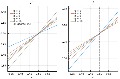
This implies that when the cost of reserve management goes up, the exchange rate appreciates less and the government accumulates reserves at a slower pace.
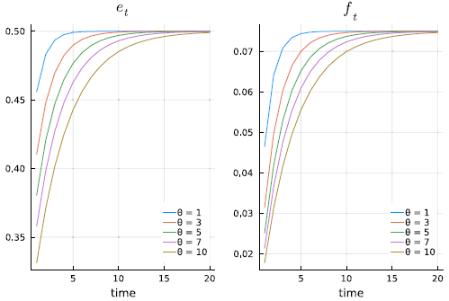
Assume parameter values as in Table 1. Figure 4 describes
 $e'$
and
 $f$
as functions of
 $e$
for each value of
 $\theta$
, while Figure 5 displays the corresponding time paths of exchange rates and reserve accumulations. One can see that the economy converges to the steady state at a slower pace as
 $\theta$
increases.
 $e'$
and
 $f$
as functions of
 $e$
for different values of
 $\theta$
.

Time paths of
 $e_t$
and
 $f_t$
for different values of
 $\theta$
.

C. Proof of Proposition 2
Proof. Iterate forward equation (4) and impose
 $f_{t+j+1}= f^{MP}$
for
 $j\geq 0$
 \begin{align*} e_{t+1} &= \frac {1}{\alpha +\gamma }\sum _{j=0}^\infty \left (\frac {\alpha }{\alpha +\gamma }\right )^j f^{MP} \\ & = \frac {1}{\gamma }f^{MP} \end{align*}
Hence, the exchange rate is expressed as
 \begin{align} e_t = \frac {\alpha }{\gamma (\alpha +\gamma )}{f}^{MP} +\frac {1}{\alpha +\gamma }f_t \end{align}
The choice
 $f_t$
by the Markov-Perfect policy solves
 \begin{equation*} \max _{f_t} -U(e_t,f_t)+ \sum _{s= t+1}^{\infty }\beta ^{s-t}\left \{- U\left (\frac {1}{\gamma }{f}^{MP},f^{MP}\right )\right \} \end{equation*}
subject to (12).
The first-order condition to this problem gives
 \begin{align*} -\frac {1}{\alpha +\gamma } \left (\frac {\alpha }{\gamma (\alpha +\gamma )}f^{MP} + \frac {1}{\alpha +\gamma }f_t -\bar {e}\right ) -\theta f_t = 0 \end{align*}
Imposing
 $f_t=f^{MP}$
and rearranging,
 \begin{align*} f^{MP} &= \left (\frac {\gamma }{1+\theta \gamma (\alpha +\gamma )}\right )\bar {e} \\ &= \gamma \omega ^{MP} \bar {e} \end{align*}
where
 $\omega ^{MP}=1/\left (1+\theta \gamma (\alpha +\gamma )\right )$
. The associated exchange rate is
 \begin{align*} {e}^{MP}_t =\omega ^{MP}\bar {e} \end{align*}
D. Extension: model with uncertainty
Consider an extension of the model that incorporates capital flow shocks
 $w_t$
, an iid process following the standard normal distribution. The capital flow equation becomes
 \begin{align} \Delta k_t = \alpha (e_t - e_{t+1}) + \sigma w_t \end{align}
where
 $\sigma \gt 0$
, and hence (4) becomes
 \begin{align} e_t &= \frac {1}{\alpha +\gamma }\left (\alpha e_{t+1} + \Delta R_t - \sigma w_t\right ) \end{align}
while other equilibrium conditions (5) and (6) remain the same. Thus, the Ramsey problem is to solve
 \begin{align*} \max _{\vec {e},\vec {f}} \mathbb{E}_0\sum _{t=0}^\infty \beta ^t\left \{-U(e_t,f_t)\right \} \end{align*}
subject to the equilibrium conditions (5), (6), and (14). Since the model is linear-quadratic, the certainty equivalence result holds, that is,
 $f_t$
is the same as in the baseline case without uncertainty.