


It is an established finding that depression is associated with deficits in cognitive function (Burt, Zembar, & Niederehe, Reference Burt, Zembar and Niederehe1995; McDermott & Ebmeier, Reference McDermott and Ebmeier2009; Rock, Roiser, Riedel, & Blackwell, Reference Rock, Roiser, Riedel and Blackwell2014; Snyder, Reference Snyder2013) and executive function (EF) (Snyder, Reference Snyder2013). EFs refer to the set of high-level cognitive processes that control ongoing behaviour to allow a goal-directed action (Miyake et al., Reference Miyake, Friedman, Emerson, Witzkia, Howertera and Wager2000; Norman & Shallice, Reference Norman, Shallice, Davidson, Schwartz and Shapiro1986) by regulating subordinate cognitive processes (see e.g. Logan & Gordon, Reference Logan and Gordon2001). The finding that EFs are impaired in depression is perhaps not surprising given that the prefrontal cortex – an essential region for efficient executive functioning (Stuss & Knight, Reference Stuss and Knight2002) – has been shown to function hypoactively in depressed individuals (Levin, Heller, Mohanty, Herrington, & Miller, Reference Levin, Heller, Mohanty, Herrington and Miller2007).
Assessing the effects of clinical disorders on executive functioning is complicated by the fact that EFs themselves are not directly observable; as they are higher-order processes that act on lower-order processes (e.g., such as perceptual processes), one can only infer the influence and efficacy of EFs by observing changes in manifest variables, such as response time (RT; Logan & Gordon, Reference Logan and Gordon2001; Miyake et al., Reference Miyake, Friedman, Emerson, Witzkia, Howertera and Wager2000). Importantly, though, changes in EF and subordinate processes can independently influence manifest variables. This complicates matters because a clinical disorder that negatively affects a subordinate process may lead to prolonged RT in a clinical group in comparison to a control group; the impaired RT could mistakenly be taken as evidence of impaired EFs in the clinical group.
One solution to this task impurity problem (Miyake et al., Reference Miyake, Friedman, Emerson, Witzkia, Howertera and Wager2000) is to fit computational cognitive models to data from clinical and control groups (Farrell & Lewandowsky, Reference Farrell and Lewandowsky2010; Lewandowsky & Farrell, Reference Lewandowsky and Farrell2010). Such models of EF will have parameters that reflect higher-order processes (such as control processes) and lower-order processes (such as the strength of perceptual representations), allowing one to distinguish between effects on EFs and subordinate processes, and how these processes change across conditions and clinical groups.
Modelling the effects of depression on flanker task performance
One popular measure of a component of EF – visual selective attention – is the Eriksen flanker task (Eriksen & Eriksen, Reference Eriksen and Eriksen1974). In this task, participants are presented with a series of arrows (for example) and must respond to the direction of the central arrow (left v. right). On some trials, the central arrow is flanked by arrows that point in the opposite direction to that of the target (incongruent trials; e.g. >><>>), and on other trials the central arrow is flanked by arrows pointing in the same direction (congruent trials; e.g. <<<<<). It is a well replicated finding that incongruent trials are responded to more slowly and with poorer accuracy than congruent trials; this congruency effect is thought to reflect the interference caused by the flankers during response selection in the incongruent condition, and the time taken to overcome such interference. The magnitude of the flanker effect can thus be used to assess the efficacy of visual selective attention, with smaller values suggesting better selective attention.
Dillon et al. (Reference Dillon, Wiecki, Pechtel, Webb, Goer, Murray and Pizzagalli2015) recently utilised the flanker task to assess visual selective attention in individuals with major depressive disorder (MDD) compared to a control group. In the behavioural data, Dillon et al. (Reference Dillon, Wiecki, Pechtel, Webb, Goer, Murray and Pizzagalli2015) found those with MDD performed more slowly but also more accurately than control participants on incongruent trials. Such speed–accuracy trade-offs are notoriously difficult to interpret (see e.g. Wagenmakers, van der Maas, & Grassman, Reference Wagenmakers, van der Maas and Grassman2007; Wickelgren, Reference Wickelgren1977): slower RTs suggest poorer performance, but better accuracy suggests better performance.
Dillon et al. (Reference Dillon, Wiecki, Pechtel, Webb, Goer, Murray and Pizzagalli2015) fitted a computational model of flanker task performance – the Linear Approach to Threshold with Ergodic Rate (LATER) model (Noorani & Carpenter, Reference Noorani and Carpenter2013) – to correct RTs for both groups. This model has parameters reflecting three core cognitive processes: pre-potent response bias (the degree to which the participant is influenced by distracting flankers); response inhibition (required to resist early responding); and executive control (required to overcome the pre-potent response and respond accordingly to the central target). The results of the modelling showed reduced pre-potent response bias and slower executive control in the depressed group. Within the depressed group, there was a significant negative correlation between the speed of executive control and a questionnaire measure of anhedonia.
Modelling attentional selectivity
Given the striking speed–accuracy trade-off reported by Dillon et al., Reference Dillon, Wiecki, Pechtel, Webb, Goer, Murray and Pizzagalli2015, it is imperative to take into account both accuracy and response speed when modelling the effects of depression. It has been shown that accuracy data provides essential information – and hence, essential constraints on theoretical modelling – about the dynamics of attentional selectivity in the flanker task. Gratton, Coles, Sirevaag, and Eriksen (Reference Gratton, Coles, Sirevaag and Eriksen1998) used conditional accuracy functions (CAFs) to examine the dynamics of attentional selectivity in the flanker task. CAFs are constructed by ordering a participant's RTs for each condition (e.g. congruent trials and incongruent trials separately) from fastest to slowest, and then dividing this data into equally-sized bins. The accuracy for each bin is then plotted against the mean RT for each bin to show how accuracy changes across the RT distribution.
Gratton et al. (Reference Gratton, Coles, Sirevaag and Eriksen1998) used CAFs of flanker task performance to show that attentional selectivity improves with processing time: They reported a large congruency effect in accuracy for the fastest RT bins, but this congruency effect in accuracy reduced as RT increased. This finding is consistent with theoretical accounts of flanker task performance that assume attentional selectivity is relatively poor at early stages of processing, leading to uncertain response selection on incongruent trials as it is heavily influenced by the flanker stimuli; as processing time increases, attentional selectivity improves leading to a reduction of the influence of flanker stimuli on response selection. Note that this theoretical insight could not be established if accuracy data were not accounted for.
The current study
The purpose of the present study was to revisit the effect of depression on flanker task performance, but to fit the data two models – the dual-stage two-phase (DSTP) model of Hübner, Steinhauser, and Lehle (Reference Hübner, Steinhauser and Lehle2010) and the shrinking spotlight (SSP) model of White, Ratcliff, and Starns (Reference White, Ratcliff and Starns2011) – that were explicitly designed to jointly account for RT and accuracy performance, and thus could model the full dynamics of attentional selectivity.
Overview of the models
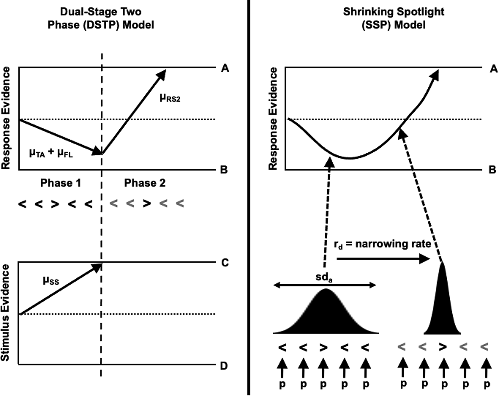
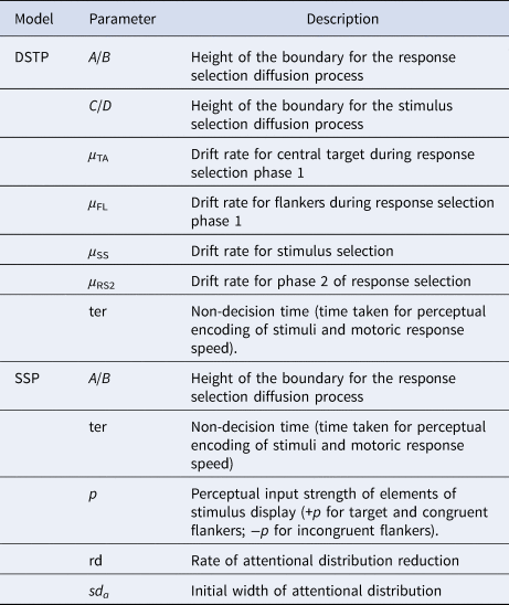
Both the DSTP and the SSP model successfully capture the improvement of attentional selectivity with processing time, but with different theoretical accounts. Figure 1 provides an overview of the main theoretical difference between the two models. A more detailed computational account of the two models is provided in online Supplementary material Appendix A; a brief description of the main parameters in each model is provided in Table 1.
Schematic overview of the response selection processes in both models. DSTP Model: The upper panel depicts the diffusion process for response selection, and the lower panel depicts the diffusion process for stimulus selection. The point in time that a stimulus is selected for further processing is depicted by the dashed vertical line. The diffusion process before this point represents the first stage of response selection, and after this point represents the second – more selective – stage of response selection. SSP Model: The upper panel depicts the diffusion process for response selection, the drift rate of which is determined by the perceptual input of stimuli that fill within the area of the attentional spotlight, depicted in the lower panel. As time progresses, the attentional spotlight becomes more focussed around the central target, meaning perceptual information from the flankers contribute less to the drift rate of response selection as time increases. Figure available at https://flickr.com/photos/150716232@N04/48957578602 under CC license https://creativecommons.org/licenses/by/2.0/.

List and brief description of model parameters in the DSTP model and the SSP model

Both models assume that response selection proceeds according to a drift-diffusion process: After perceptual encoding of the stimulus, the cognitive system accumulates (noisy) evidence over time toward one of two response boundaries (one representing a correct response, and the other representing an error response). The boundary that is reached by the diffusion process determines the model's response accuracy, and the time taken for the boundary to be reached the RT.
Both models assume early stages of response selection are influenced by both the flankers and the central target, but at later stages of processing, response selection is primarily driven by attention to the central target. The two models, however, have different assumptions as to how attentional selectivity increases over time, and how this influences response selection. The DSTP model assumes two phases to response selection: In a first phase, attentional selectivity is poor and response selection is influenced by the whole stimulus display; at a discrete point in time, the attentional system selects the central target for more-detailed processing, leading to the second phase of response selection which is influenced solely by the central target. The time taken for the system to select which stimulus to process further is also modelled by a parallel diffusion process (see Fig. 1). The SSP model also assumes that early stages of response selection are influenced by the whole stimulus display, but that attentional selectivity improves gradually over time (i.e. the attentional spotlight gradually reduces its diameter), meaning that later stages of response selection are influenced less by the flankers. The contribution of each element in the stimulus display (i.e. the central target and the flankers) is a multiplicative combination of the strength of perceptual input of the stimulus items (represented by model parameter p) and the area of the attentional spotlight currently over the stimulus items.
General method
We conducted one exploratory experiment, followed by two confirmatory (pre-registered) experiments. In this section, we provide an overview of the general method shared by all three experiments. Where relevant, we also highlight the minor differences between each experiment. All experiments were programmed and delivered using the online behavioural science platform GorillaTM (https://gorilla.sc; Anwyl-Irvine, Massonnié, Flitton, Kirkham, & Evershed, Reference Anwyl-Irvine, Massonnié, Flitton, Kirkham and Evershed2020). Participants were recruited using Prolific Academic (https://prolific.ac). This study received full ethical clearance from the Ethics Panel run by the School of Psychology at Keele University, UK (application number PS–190046). The methods and analytical strategy were pre-registered for Experiments 2 and 3 at https://aspredicted.org (see https://aspredicted.org/3hr8j.pdf and https://aspredicted.org/8eg68.pdf, respectively).
Participants
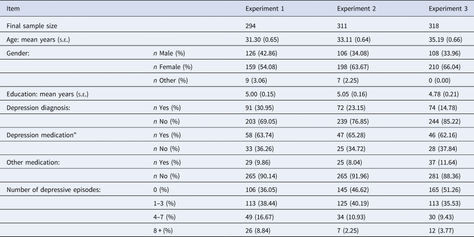
Using pre-screening tools in Prolific Academic, we limited our sample to participants residing in the UK or the USA aged between 18 and 60. Participants were screened so that they could only use a laptop or desktop machine (i.e. no mobile devices or tablet). After exclusion criteria were applied (see later section in the General Method), the final sample sizes for Experiments 1–3 were 294, 311, and 318, respectively. The demographic information of the final samples across all three experiments is shown in Table 2.
Demographics data for the sample from all experiments
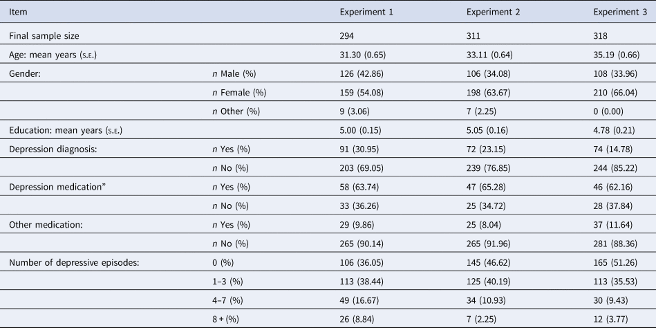
Note: s.e., standard error of the mean; n, number.
Materials and flanker task
Demographics questionnaire
Participants completed a brief questionnaire to measure some demographic information. Participants were asked to: enter their date of birth; select their gender (male–female–other); enter how many years of post-16 education they had; select whether they had a clinical diagnosis of depression (i.e. from a health professional; yes–no); if they did have depression, select whether they were currently taking medication for depression (yes–no); select whether they were taking medication for another mental health problem (yes–no; if yes, participants were asked to indicate what the mental health problem was); enter how many episodes of depression the participant had experienced over the past 2 weeks, regardless of whether they had a formal diagnosis or notFootnote 1.
Quick inventory of depressive symptomatology–self-report (QIDS–SR)
The QIDS–SR (Rush et al., Reference Rush, Trivedi, Ibrahim, Carmody, Arnow, Klein and Keller2003) is a 16-item self-report questionnaire assessing severity of depression symptoms experienced by respondents over the past 7 days. Each item relates to a particular symptom (e.g. feeling sad), and requires the participant to select one response from four options that best describes them (e.g. ‘I almost always feel sad’). The scale shows very good internal consistency and sensitivity to symptom changes (Rush et al., Reference Rush, Trivedi, Ibrahim, Carmody, Arnow, Klein and Keller2003). Scores on the quick inventory of depressive symptomatology (QIDS) range from 0 to 27 (low to high depressive symptomatology).
Snaith–Hamilton pleasure scale (SHPS)
The SHPS (Snaith et al., Reference Snaith, Hamildon, Morley, Humayan, Hargreaves and Trigwell1995) is a 14-item self-report questionnaire that probes the participant's ability to experience pleasure; the questionnaire asks participants to consider their response in relation to how they have felt in the last few days. Each item requires participants to read a statement (e.g. ‘ I would find pleasure in my hobbies and pastimes’), and to then select a response to indicate their agreement with the statement (e.g. ‘Definitely Agree, Agree, Disagree, Definitely Disagree’). We used the scoring method recommended by Franken, Rassin, and Muris (Reference Franken, Rassin and Muris2007) (Definitely Agree = 1, Agree = 2, Disagree = 3, Definitely Disagree = 4). In Experiment 1, the response options were always ordered: Definitely Disagree, Disagree, Agree, Definitely Agree. In Experiments 2 and 3, the response options were changed to match exactly the order and wording presented by Snaith et al. (Reference Snaith, Hamildon, Morley, Humayan, Hargreaves and Trigwell1995) (e.g. sometimes ‘Strongly’ was used instead of ‘Definitely’; sometime ‘Strongly Agree’ was the first option, etc.).
Attention checks
In Experiments 2 and 3, we wanted to exclude participants who were demonstrably not paying attention to the questionnaire items. Thus, we used an attention check embedded within the SHPS questionnaire. Specifically, the final item on the SHPS read, ‘It is important that you pay attention to this study. Please select Disagree’ Footnote 2. Participants who failed to select this response option were excluded from the final sample.
Flanker tasks
We used the same trial timings for all trials (practice and main blocks) for all experiments. On each trial, a black fixation cross was presented on the centre of the screen for 500 ms; this was immediately followed by a presentation of the flanker stimulus, which was displayed until the participant made a response. After a response was registered, the fixation cross for the next trial was presented. The flanker stimuli used in Experiments 1 and 2 were arrows, presented in black font. The central target could face either left or right. This central target was flanked by two arrows on either side; these flankers all faced the same direction as each other. On congruent trials, the flankers faced the same direction as the target (e.g. <<<<<); on incongruent trials, the flankers faced the opposite direction as the target (e.g. >><>>). The participants' task was to make a spatially-congruent response as to the direction of the central target, pressing the ‘Z’ key for a left response, and the ‘M’ key for the right response. In Experiment 3, we used the letters ‘K’ and ‘A’ as stimuli (e.g. a congruent trial would be KKKKK, and an incongruent trial would be AAKAA). The participants' task was to judge the identity of the central letter by pressing the ‘A’ key if the letter was A, and the ‘K’ key if the letter was K. In all experiments, the stimulus from each trial was selected randomly from the total set of four possible stimuli, with the constraint that all stimuli occurred equally often in each block. Participants were asked to respond as quickly and as accurately as possible as soon as the stimulus appeared, using the index finger of each hand for their responses.
In all experiments, participants took part in 16 practice trials before commencing the main flanker blocks. The number and duration of the flanker blocks differed across experiments: in Experiment 1, there were 6 blocks of 60 trials; in Experiments 2 and 3 there were 8 blocks of 60 trials. Participants were provided feedback on their accuracy in the practice blocks: on correct trials, a green tick would overlay the central target; on incorrect responses, a red cross would overlay the central target.
Procedure
The same procedure occurred in all three experiments. Upon entering the study online, participants were presented with an information screen that provided general information about the study so they could decide whether they wished to take part, at which point participants were presented with a screen on which they provided informed consent.
Participants then completed the brief demographics questionnaire. At this point, the experimental software randomised the participant to one of four presentation orders, which counterbalanced the order of presentation of the questionnaires and the flanker task: (1) flanker task – QIDS – SHPS; (2) flanker task – SHPS – QIDS; (3) QIDS – SHPS – flanker task; (4) SHPS – QIDS – flanker task.
Before completing the flanker task, participants were presented with a full instruction screen that provided complete instructions for how to complete the flanker task. This was followed by a brief practice block before moving on to the main blocks. After each block, participants were invited to take a short (self-paced) break. The QIDS questionnaire was presented on four consecutive screens, with four questions per screen. Participants indicated their response to each item by selecting the relevant response clicking a radio button with their mouse; participants could change their response freely until they proceeded to the next screen. The SHPS questionnaire was presented across four screens, with four items on the first three screens, and two items on the last screen. Responses were again indicated via radio buttons. Once participants had completed all elements of the study, they were presented with a debrief screen, which provided detailed information about the nature of the experiment.
Quality checks and data exclusion
Before analysing the data, we conducted some quality checks on the data and removed some participants with reference to pre-defined (and pre-registered in Experiments 2 and 3) exclusion criteria. In Experiments 2 and 3, individuals who failed the attention check embedded within the SHPS questionnaire were removed. Responses to the questionnaires were also examined for ‘straight-lining’ (e.g. only selecting the left-most response to all items); participants who showed straight-lining to all questions for both questionnaires were removed.
For the behavioural data, we removed participants who had a mean accuracy lower than 80%. For the RT analysis, error trials were removed; RTs were trimmed by removing RTs shorter than 250 ms and longer than 1500 ms. In cases where trimming removed more than 25% of an individual's data, that participant was removed.
Results
Analytical strategy
All inferential analyses utilised a Bayesian regression approach using the brms package (Bürkner, Reference Bürkner2017) in R (R Core Team, 2017). Default regularising priors from the brms package were used throughout. Unless otherwise stated, the response variable in the regressions was modelled as being distributed normally. Predictor variables were considered to contribute meaningfully if their 95% credible intervals (CI) did not include zeroFootnote 3. Each statistical model was fit using brms by running four chains of the ‘no U-turn’ sampling (NUTS) of the posterior distribution for each parameter, with 4000 samples per chain (the first 2000 samples of which counting as ‘burn-in’); we inspected the chains to ensure convergence, and all $\hat{R}$ were close to 1.
Questionnaire scores
There were good variability and ranges of scores across all three experiments for both the QIDS (Experiment 1: range = 0–25, M = 11.27, s.d. = 6.12; Experiment 2: range = 0–24, mean = 9.27, s.d. = 5.26; Experiment 3: range = 0–24, mean = 9.15, s.d. = 5.31) and the SHPS scores (Experiment 1: range = 14–50, mean = 27.91, s.d. = 7.69; Experiment 2: range = 14–44, mean = 28.02, s.d. = 6.25; Experiment 3: range = 14–51, mean = 27.08, s.d. = 6.76). Bayesian regressions showed that QIDS scores were positively predicted by SHPS scores across all three experiments, indicating good convergence of the measures [Experiment 1: β Intercept = 7.63, 95% CI(6.82, 8.43), β SHPS = 1.11 (0.95, 1.28); Experiment 2: β Intercept = −5.29 (−7.37, −3.16), β SHPS = 0.52 (0.44, 0.59); Experiment 3: β Intercept = −4.22 (−6.08, −2.33), β SHPS = 0.49 (0.43, 0.56)]Footnote 4.
In the study of Dillon et al. (Reference Dillon, Wiecki, Pechtel, Webb, Goer, Murray and Pizzagalli2015), participants were included in the ‘depressed’ condition if they had – together with meeting other diagnostic criteria – a QIDS score of 14 or more (which reflects moderate depression); inclusion in the control group required a QIDS score lower than 8. In our samples, there were 109, 67, and 70 who scored above 14 in the QIDS in Experiments 1–3, respectively; these numbers were 88, 122, and 137 for those scoring below 8. Also, our sample contained a reasonable proportion of participants who self-declared a clinical diagnosis of depression (see Table 2). Thus our samples contained a good spread of depression symptomology.
Behavioural results
Before presenting the results of the computational modelling, we provide an overview of the behavioural results to explore the magnitude of the flanker effect in both RT and error, as well as the relationship between these outcomes and questionnaire scores.
Flanker effect in RT and accuracy
For the RT analysis, a Bayesian regression was conducted with trial-level RT as the outcome variable and congruency as the predictor variable; the outcome variable was modelled as an ex-Gaussian distributionFootnote 5. There was a large flanker effect in RT in all three experiments [Experiment 1: β incongruent = 48 (37, 59); Experiment 2: β incongruent = 53 (44, 63); Experiment 3: β incongruent = 30 (21, 39)]. The accuracy analysis utilised a similar Bayesian regression, but the outcome variable (proportion correct) was modelled as a skewed normal distribution. Again, there was a large flanker effect in all three experiments [Experiment 1: β incongruent = −0.01 (−0.014, −0.006); Experiment 2: β incongruent = −0.01 (−0.014, −0.007); Experiment 3: β incongruent = −0.01 (−0.015, −0.008)].
Predicting behavioural data from QIDS and SHPS
We performed a series of Bayesian regressions to explore whether the behavioural flanker effect was predicted by scores on the QIDS and SHPS. Results showed that the RT flanker effect was not predicted by QIDS scores [Experiment 1: β QIDS = 0.02 (−0.53, 0.58); Experiment 2: β QIDS = 0.23 (−0.41, 0.89); Experiment 3: β QIDS = 0.11 (−0.22, 0.44)] or SHPS scores [Experiment 1: β SHPS = −0.65 (−1.67, 0.40); Experiment 2: β SHPS = −0.17 (−0.71, 0.38); Experiment 3: β SHPS = −0.04 (−0.29, 0.21)]. The accuracy flanker effect was also not predicted by either QIDS [Experiment 1: βQIDS = −0.0003 (−0.0010, 0.0005); Experiment 2: β QIDS = −0.0003 (−0.0009, 0.0003); Experiment 3: β QIDS = 0.0001 (−0.0004, 0.0007)] or SHPS scores [Experiment 1: β SHPS = −0.0003 (−0.0015, 0.0009); Experiment 2: β SHPS = 0.0000 (−0.0005, 0.0004); Experiment 3: β SHPS = 0.0002 (−0.0001, 0.0006)]. See online Supplementary material Appendix C for more details.
Modelling results
We fit the DSTP and SSP models to individual participant data using the flanker package (Grange, Reference Grange2016). The models were fitted to trial-level RT and accuracy data. Full details of the fit routine and assessment of the goodness of fits (which were good) for both models can be found in online Supplementary material Appendix D. We also report in Supplementary material Appendix D formal model comparison tests of whether one model provided superior fits over the other. We found that the SSP model was superior for Experiments 1 and 2, and the DSTP model was superior for Experiment 3.
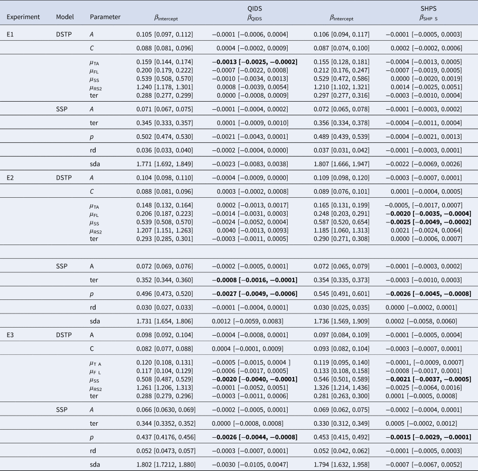
To assess whether model parameters were predicted by QIDS and SHPS scores, a series of Bayesian regressions were conducted; the outcome variables in all regressions were modelled as a skewed normal distribution. For ease of exposition, we present the regression coefficients for all models and all experiments in Table 3; plots of all Bayesian regressions can be found in the online Supplementary material Appendix E.
Bayesian regression coefficients (with 95% CIs) predicting DSTP and SSP model parameters from QIDS and SHPS questionnaire scores across all experiments

DSTP model
No DSTP parameter was consistently predicted by depression scores (QIDS) across the three experiments. Although the parameter μ TA was negatively associated with depression symptoms in Experiment 1, this did not replicate in Experiment 2 or 3. Likewise, although the parameter μ SS was negatively associated with depression in Experiment 3, we did not find this to be the case in the first two experiments. However, this parameter was negatively associated with anhedonia (SHPS) in Experiments 2 and 3, but this was not evident in Experiment 1. This suggests that the time is taken for the cognitive system to select the central target for further processing – in the model, reflected by the drift rate shown in the lower panel of the DSTP schematic shown in Fig. 1 – is longer for those with higher levels of anhedonia. Parameter μ FL was negatively associated with anhedonia in Experiment 2, but not in Experiment 1 or 3.
SSP model
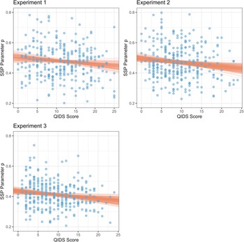
We found that the SSP model parameter p was consistently (negatively) predicted by depression (QIDS) across all three experiments [the 95%CI for this regression coefficient in Experiment 1 only just included zero, βQIDS = −0.002 (−0.0043, 0.0001)]. This relationship is plotted in Fig. 2. This parameter – which reflects the perceptual input strength of each element of the encoded flanker stimulus – was lower in individuals with higher levels of depression symptoms. This parameter was also negatively predicted by measures of anhedonia in Experiments 2 and 3, but not in Experiment 1. No other SSP parameters were predicted by QIDS or SHPS scores.
Relationship between the SSP model parameter p and measure of depression from the QIDS questionnaire for Experiments 1–3. Points represent participant data; the lines represent 200 draws from the posterior distribution for the statistical models Experiments 1–3.

General discussion
The current study aimed to extend the findings of Dillon et al. (Reference Dillon, Wiecki, Pechtel, Webb, Goer, Murray and Pizzagalli2015) by fitting two computational models able to account jointly for accuracy and RT performance, as well as the ubiquitous improvement of attentional selectivity with time found in the flanker task. Specifically, we fit the DSTP model (Hübner et al., Reference Hübner, Steinhauser and Lehle2010) and the SSP model (White et al., Reference White, Ratcliff and Starns2011) to data from three large-scale online experiments where self-reported measures of depression symptomology (as measured by the QIDS) and anhedonia (as measured by the SHPS) were recorded.
In terms of behavioural data, we did not find any relationship between depression symptomology or anhedonia on any of the primary dependent variables at the mean level, in contrast to the findings of Dillon et al. (Reference Dillon, Wiecki, Pechtel, Webb, Goer, Murray and Pizzagalli2015). However, in the supplementary analysis (see online Supplementary material Appendix F) where we grouped participants into high-QIDS (a score of 14 or above) and low-QIDS (a score below 8), group differences emerged in the conditional accuracy functions, with high-QIDS participants showing poorer attentional selectivity at faster responses. As the DSTP and SSP models are fitted to conditional accuracy functions (combining RT and accuracy) and cumulative distribution functions (which describe the whole of the correct RT distribution), this analysis suggests that there were effects of depression that the modelling could be useful to describe.
No DSTP model parameter was consistently associated with depression or anhedonia across any of the three experiments. In contrast, however, the SSP model parameter p was consistently negatively associated with depression (and anhedonia in Experiments 2 and 3). This model parameter reflects the strength of the perceptual input of each item in the stimulus display (see Supplementary material Appendix A for more details), suggesting this input strength is weaker in those with higher levels of depression. In an experimental validation of the SSP model, the p parameter has been shown to vary systematically with the intensity and contrast of presented visual stimuli (Servant, Montagnini, & Burle, Reference Servant, Montagnini and Burle2014), suggesting it can index perceptual index strength accurately.
Do perceptual deficits exacerbate control problems in depression?
Although some evidence exists from psychophysical experiments that depression is associated with deficits in perceptual processing (e.g. Bubl, Kern, Ebert, Bach, & van Elst, Reference Bubl, Kern, Ebert, Bach and van Elst2010; Bubl, van Elst, Gondan, Ebert, & Greenle, Reference Bubl, van Elst, Gondan, Ebert and Greenle2009; Normann, Schmitz, Furmaier, Doing, & Bach, Reference Normann, Schmitz, Furmaier, Doing and Bach2007) – and that depression can lead to poorer visual search times (Maekawa, Anderson, de Brecht, & Yamagishi, Reference Maekawa, Anderson, de Brecht and Yamagishi2018) – to our knowledge our findings are the first to report perceptual deficits in depression captured by a computational model of higher-order cognition. This finding is of significance because the models capture how perceptual information and higher-order attentional processes interact to produce successful performance. Indeed, this is one of the many advantages of utilising computational models of cognition to probe clinical disorders (see e.g. White, Ratcliff, Vasey, & McKoon, Reference White, Ratcliff, Vasey and McKoon2010) because we can tease apart the effects of depression on higher-order processes and lower-order, subordinate, processes. The findings from the current study are striking as they suggest that depression symptomology is not negatively affecting attentional processes per se, but instead suggests depressed participants show deficits in a lower-order, subordinate, process of perceptual representationFootnote 6.
This raises the intriguing hypothesis – which should be the subject of future work – that the cognitive control deficits in depression found in recent studies (Burt et al., Reference Burt, Zembar and Niederehe1995; McDermott & Ebmeier, Reference McDermott and Ebmeier2009; Rock et al., Reference Rock, Roiser, Riedel and Blackwell2014; Snyder, Reference Snyder2013) are problems that are exacerbated by perceptual deficits: If individuals with depression have weaker perceptual representations, then the cognitive system has weaker information with which to work when cognitive control is required, leading to less efficient control.
Indeed, this hypothesis is not inconsistent with the findings of Dillon et al. (Reference Dillon, Wiecki, Pechtel, Webb, Goer, Murray and Pizzagalli2015), who found significantly reduced pre-potent response bias in the depressed group. This parameter reflects the negative influence of flankers on incongruent trials, which push the cognitive system towards an error response. Finding a reduction of this parameter in depressed participants could be interpreted as a weaker perceptual representation of the flankers, which would mean they influenced behaviour less than in control participants. In the extreme version of this hypothesis, perceptual deficits might exclusively explain control problems in depression.
Future work should combine computational modelling with experimental manipulation of perceptual properties of stimulus displays to test this hypothesis further. In addition, the emotional nature of the stimuli should be considered in future work. We used emotionally neutral stimuli. A substantial body of literature demonstrates that patients with depression show mood-congruent emotion processing bias; specifically, negative stimuli (e.g. negative faces) are processed more rapidly and deeply, whilst processing of positive stimuli seems to be impaired (e.g. Gotlib, Krasnoperova, Yue, & Joormann, Reference Gotlib, Krasnoperova, Yue and Joormann2004; Stuhrmann, Suslow, & Dannlowski, Reference Stuhrmann, Suslow and Dannlowski2011). Furthermore, evidence indicates that these impairments in emotion processing can be reversed with psychotropic treatment (Fu et al., Reference Fu, Williams, Brammer, Suckling, Kim, Cleare and Bullmore2007). Future work should thus explore whether our general pattern of results replicates using emotional stimuli.
Limitations
The study has several limitations that should be considered. Firstly, due to the many model parameters, our analyses – and thus our conclusions – rest on the outcome of multiple comparisons, so we should be cautious of our Type-1 error rate. Whilst a valid concern, we believe that our main finding of reduced SSP model parameter p with depression severity is robust. It replicated across (pre-registered) experiments, across depressive symptom measures, and was also evident in the group analysis based on extreme QIDS scores (Supplementary material Appendix F).
Secondly, we used an online sample rather than using lab-condition testing. However, there is good evidence that online recruitment can provide quality data for cognitive tasks (Crump, McDonnell, & Gureckis, Reference Crump, McDonnell and Gureckis2013). Our behavioural data quality was also very high (see online Supplementary material Appendix C), suggesting that this potential limitation has not impacted on our conclusions.
Finally, we did not recruit a clinical sample; however, we had many participants in all three Experiments who scored above 14 on the QIDS, which Dillon et al. (Reference Dillon, Wiecki, Pechtel, Webb, Goer, Murray and Pizzagalli2015) used as an inclusion criterion in their ‘depressed’ group. Therefore, although not from a clinical sample, we had a significant subset in each experiment that exhibited moderate depression on the QIDS. As we show in online Supplementary analysis Appendix F, when we compare this high-QIDS group with a low-QIDS group (QIDS score lower than 8 Dillon et al., Reference Dillon, Wiecki, Pechtel, Webb, Goer, Murray and Pizzagalli2015), our main conclusions of lower p SSP parameter values in higher depression stands. However, when we grouped participants into those who declared a clinical diagnosis of depression and those who declared no such diagnosis, we found no consistent group differences. Although there are many advantages to conducting research on a large non-clinical sample (see e.g. the Research Domain Criteria set out by the NIMH: https://www.nimh.nih.gov/research/research-funded-by-nimh/rdoc/index.shtml), further tests of the ‘perceptual-hypothesis’ should be conducted on individuals with diagnosed MDD. Computational modelling will be essential to address this hypothesis.
Supplementary material
The supplementary material for this article can be found at https://doi.org/10.1017/S0033291720002652.
Data
All raw data, analysis scripts, and computer code for the modelling can be downloaded from https://osf.io/rufp9/. The experimental materials for Experiment 1 can be downloaded from https://gorilla.sc/openmaterials/43291, for Experiment 2 from https://gorilla.sc/openmaterials/55094, and for Experiment 3 from https://gorilla.sc/openmaterials/55095.
Acknowledgements
None.
Financial support
This research received no specific grant from any funding agency, commercial, or not-for-profit sectors.
Conflict of interest
None.
Ethical standards
The authors assert that all procedures contributing to this work comply with the ethical standards of the relevant national and institutional committees on human experimentation and with the Helsinki Declaration of 1975, as revised in 2008.