Introduction
The Southern Ocean (SO) and adjacent seas, such as the Ross and Weddell seas, are key regions for understanding the connections between the atmosphere and the ocean in climatic scales. Changes in the SO heat content have the potential to modify the Meridional Overturning Circulation (MOC) and influence the world's oceans (Stössel & Kim Reference Stössel and Kim2001). The modification of the properties, such as temperature and salinity, of the water masses formed in the SO and around the Antarctic affect both the MOC intensity and pathways. However, it is still a matter of debate what the main driving mechanisms for the observed variability in the water mass formation sites are, and what the possible impacts of ongoing climate changes are. Changes in the heat content within these areas can be a consequence of anomalous surface fluxes at the sea-air interface, anomalous lateral oceanic fluxes or, possibly, a combination of both (e.g. Fyfe et al. Reference Fyfe, Saenko, Zickfeld, Eby and Weaver2007, Farneti & Delworth Reference Farneti and Delworth2010). A clear picture of what are the contributions of the mean atmospheric and oceanic heat fluxes is necessary in order to explain the variability in the heat content of the SO and adjacent southern seas.
The major oceanographic feature of the SO is the Antarctic Circumpolar Current (ACC). This is the longest and strongest current system of the world ocean, flowing eastward around the globe, with a volume transport of approximately 130–140 Sv (1 Sv ≈ 106 m3 s-1) at the Drake Passage (Olbers et al. Reference Olbers, Borowski, Völker and Wölf2004). The ACC has been reported as intrinsically baroclinically unstable in several regions. Mainly with the advent of satellite altimetry, significant mesoscale activity has been observed to occur in the SO, especially in the ACC domain.
Several reviews agree that the mesoscale activity is a key phenomenon in the dynamic balance of the ACC (e.g. Rintoul et al. Reference Rintoul, Hughes and Olbers2001, Olbers et al. Reference Olbers, Borowski, Völker and Wölf2004). Indeed, mesoscale eddies have been reported to have an important role in the maintenance of the vertical frontal structure of the ACC, transporting cold water equator-ward and warm water pole-ward (Karsten et al. Reference Karsten, Jones and Marshall2002). Individual eddies were observed to flow eastward with the main flow of the ACC and to present an important contribution to the meridional heat flux (Chelton et al. Reference Chelton, Schlax and Samelson2011). It is believed that the eddy activity plays a central role in the Deacon cell of meridional circulation, compensating the water transported northward within the Ekman layer (Karsten & Marshall Reference Karsten and Marshall2002, Karsten et al. Reference Karsten, Jones and Marshall2002).
The investigation of the SO circulation response to the strengthening of the westerly winds projected by IPCC AR4 report climate scenarios have been an active theme of research (e.g. Meredith & Hogg Reference Meredith and Hogg2006, Fyfe et al. Reference Fyfe, Saenko, Zickfeld, Eby and Weaver2007). Results from eddy resolving numerical simulations indicate that the observed increase in the northward Ekman transport should be compensated by an intensification of southward eddy fluxes, resulting in little changes in the mean overturning (Screen et al. Reference Screen, Gillet, Stevens, Marshall and Roscoe2009). However, analysis based on coarse resolution models that do not explicitly resolve the eddy activity suggest an increase of the subpolar upwelling cell and, consequently, in the upwelling of deep carbon rich waters south of the ACC (Saenko et al. Reference Saenko, Fyfe and England2005). In fact, observations show a significant modification in the SO properties. For example, using the Argo profiling floats data, Böning et al. (Reference Böning, Dispert, Visbeck, Rintoul and Schwarzkopf2008) observed coherent hemispheric scale warming and freshening trends that extend to depths of more than 1000 m. These changes are consistent with a southward migration of the isopycnal surfaces by about 50 km as a consequence of the westerly winds intensification. The variability of the cross-frontal heat flux, however, is still a matter of debate.
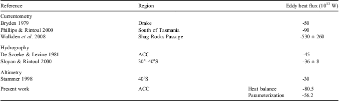
Following de Szoeke & Levine (Reference De Szoeke and Levine1981) the net heat flux across the Polar Front, the southern branch of the ACC, can be expressed as the sum of a mean geostrophic transport, an Ekman layer contribution related to the wind stress at the surface, and an eddy component. According to these authors, based on historic estimates of the SO winds and mean ocean state in the region, Ekman fluxes account for ∼ 15 x 1013 W to the north while the geostrophic transport is negligible. A southward eddy heat flux of ∼ 45 x 1013 W is then needed in order to balance the ∼ 30 x 1013 W lost from the ocean to the atmosphere south of the Polar Front.
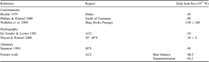
This indirect calculation, however, should be seen as a first order estimation of the real fluxes. Several authors have tried to obtain direct measurements of the southward eddy heat flux (Table I). The length of the region to be covered, the geographical variability of the fluxes, and the inhospitable conditions in the SO make this a very difficult task to be fulfilled. For this reason, most studies to date are based on satellite data or on the extrapolation of local in situ data to the total length of the ACC (e.g. Stammer Reference Stammer1998, Phillips & Rintoul Reference Phillips and Rintoul2000).
Heat flux in the Southern Ocean from distinct databases. The results are organized by the kind of data used in the calculations of the heat flux. ACC=Antarctic Circumpolar Current.
The objective of the present work is to use modern datasets that better represent the real ocean state, wind stress and ocean surface fluxes, to provide new estimates for the eddy diffusivity and eddy heat flux in the SO, particularly on the Polar Front region. Two distinct methodologies are compared. First, we revisit the work done by de Szoeke & Levine (Reference De Szoeke and Levine1981), estimating the mean components of a heat balance equation. Then, we apply a parameterization scheme discussed by Holloway & Kristmannsson (Reference Holloway and Kristmannsson1984) and Holloway (Reference Holloway1986), based on sea level anomaly (SLA) data. Both mean annual and monthly fluxes are calculated. The annual mean heat flux from the parameterization is compared with the heat balance results, and the monthly mean estimates are used to access the temporal variability.
This paper is organized as followed: in the next section, we describe the datasets used. The heat balance based in the de Szoeke & Levine (Reference De Szoeke and Levine1981) work and the parameterization are briefly described in the Methods section. Our results are then presented and discussed, followed by conclusions.
Datasets
The study domain corresponds to the SO, defined here as the circumpolar region between 30°S and the Antarctic continent. For this region, hydrographic, sea surface height (SSH), wind stress, wind speed and surface heat flux data from different sources are used. The time interval from January 2006–December 2009 is chosen to guarantee a sufficient data coverage of the upper 2000 m of the water column by the Argo program.
Argo is a global ocean observing system for the 21st century (www.argo.net) which is now the major and only systematic source of information and data over the ocean's interior. Approximately 3000 profiling floats are used to prescribe 3° x 3° x 10-day resolution array between 60°S and 60°N. These autonomous floats measure temperature and salinity throughout the global oceans down to 2000 m depth, every ten days. With Argo, a more homogenized global distribution of in situ measurements exists. Especially in the Southern Ocean sector where historical sampling is mostly reduced and biased in the summer months (von Schuckmann & Le Traon Reference Von Schuckmann and Le Traon2011). This rapidly changed at the end of 2006 when Argo sampling was almost complete. The sampling characteristics of Argo allowed for the first time to capture the seasonal and interannual variability of the global ocean circulation, with an especial improvement in the Southern Ocean sector.
The Argo climatology used in this study is based on the Argo data downloaded from the Coriolis data centre (www.coriolis.eu.org, accessed April 2011). The database underwent delayed mode quality control procedures and was released in June 2010 for the 2005–09 period. The datasets are processed by the tool “ISAS-STD” (Gaillard Reference Gaillard2010) which reads the selected variable, performs a climatological test, interpolates on standard levels and evaluates monthly gridded fields of temperature and salinity via optimal analysis (von Schuckmann et al. Reference Von Schuckmann, Gaillard and Le Traon2009). An Argo climatology based on the gridded fields of the years 2006–09 and monthly mean fields are evaluated from this database. The climatology grid was designed to match the SLA grid.
Sea surface height data from the AVISO delayed time reference product (http://www.aviso.oceanobs.com/, accessed April 2011) was downloaded for the same period of the Argo data. It corresponds to a merged satellite product, projected on a 1/3° horizontal resolution Mercator grid, in time intervals of seven days. Sea Level Anomalies were obtained by subtracting the temporal mean SSH (2006–09) from each grid point. A high pass Hanning filter with a window of 175 days was used to remove seasonal and interannual signals. A lanczos filter was applied to eliminate variability with length scales larger than 1000 km. Thus, the mesoscale variability, that is believed to be the dominant process in the eddy heat flux (Rintoul et al. Reference Rintoul, Hughes and Olbers2001), is highlighted in the dataset.
Wind stress, wind speed and total surface heat flux reanalysis results from the ERA-Interim reanalysis were obtained from the ECMWF data server (www.ecmwf.int/research/era/do/get/era-interim, accessed April 2011). These fields are provided with a 1.5° horizontal resolution every three hours. The ERA-Interim is a state-of-the-art extended reanalysis that is planned to replace the ERA-40. It presents a systematic better performance in comparison to the previous version, especially for the Southern Hemisphere. A complete description of this product was provided by Simmons et al. (Reference Simmons, Uppala, Dee and Kobayashi2006).
Methods
Definition of the Polar Front
The ACC is defined as a series of fragmented jets corresponding to distinct oceanic fronts, both at the surface and subsurface layers. Two major fronts can be used to delimit its surface meridional extent: the sub-Antarctic Front to the north and the Polar Front to the south, whose geographical positions can be determined from sea surface temperature (Orsi et al. Reference Orsi, Whitworth and Nowlin1995). In the present work, the Polar Front is used to delimit a circumpolar path for the heat flux calculation.
Different from Orsi et al. (Reference Orsi, Whitworth and Nowlin1995), in the present study the Polar Front position was defined by a vertical mean potential temperature isoline or isotherm, following de Szoeke & Levine (Reference De Szoeke and Levine1981). This definition allows an important simplification in the heat flux integration, eliminating the barotropic contribution. The use of the Polar Front instead of a constant latitude circle, traditionally used in balance calculations, minimizes the contamination from the mean flow in the calculated eddy fluxes, since the integration path approximately follows the mean current position. Since the results of the balance are sensitive to the choice of the isotherm, values between 1°C and 5°C with 0.1°C intervals were used in the integration of the heat balance equation (see next section).
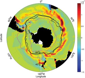
For a detailed analysis and comparison between the heat balance and the parameterization scheme results, a particular isotherm was select to represent the Polar Front based on two criteria: 1) the isotherm should coincide with the southern limit of the maximum mean temperature gradient area, representing the region of large isopycnal slope of the Polar Front, and 2) the isotherm should present a reasonable agreement with the Polar Front position calculated by Orsi et al. (Reference Orsi, Whitworth and Nowlin1995) based on a hydrographic climatology. Using these criteria, we select the 2.6°C isotherm to represent the Polar Front position. Figure 1 shows the position of the estimated Polar Front with the mean potential temperature gradients obtained from the Argo climatology. The 1°C (to the south) and 5°C (to the north) isotherms are illustrated in this figure to represent the total area comprehended by the isotherms for the heat balance calculation.
Gradient of the vertical mean potential temperature (°C m-1). The black continuous line indicates the position of the Polar Front calculated in the present work. The black dashed line corresponds to the Polar Front calculated by Orsi et al. (Reference Orsi, Whitworth and Nowlin1995). The 1°C (northern) and 5°C (southern) vertical mean isotherms are also presented to indicate the region where the heat balance is calculated (magenta dashed contours).

The annual mean position of the Polar Front was obtained from the Argo climatology, while monthly positions were calculated from the monthly mean Argo gridded product.
Heat balance
Following the methodology originally proposed by de Szoeke & Levine (Reference De Szoeke and Levine1981), we applied the idea of a circumpolar heat balance integration along the mean isotherms representing oceanic fronts, using the Argo climatology. The objective is to directly calculate the contribution of the mean barotropic (Fbt) and baroclinic (Fbc) geostrophic transports, and of the Ekman layer (Fek) transport to the heat balance expressed by:
 $${{{\rm F}_{{\bf {{bc}}}}}\,{\bf {{ + }}}\,{{{\rm {{F}}}}_{{\rm {{bt}}}}}\,{{{ + }}}\,{{{\rm {{F}}}}_{{\rm {{ek}}}}}\,{\rm {{ + }}}\,{{{\rm {{F}}}}_e}\,{\bf {{ = }}}\,{\rm {{Q}}}},\eqno\rm$$
in order to obtain an indirect estimate of the eddy (Fe) contribution, as the residual heat flux necessary to compensate the heat lost to the atmosphere (Q) south of the circumpolar path of integration.
Since this path of integration is a circumpolar section of constant mean potential temperature, we subtract this mean value from the potential temperature at each depth along the front, ensuring that the barotropic contribution to the total heat flux in the balance is zero. For the baroclinic transport we applied the same relation proposed by de Szoeke & Levine (Reference De Szoeke and Levine1981) to the Argo climatology potential temperatures and derived geostrophic currents to estimate the heat flux. As demonstrated by these authors, using a path of constant mean potential temperature leads to computed fluxes that are independent of a reference depth.
The Ekman layer heat flux is obtained from the monthly mean ERA-Interim wind stress and the monthly Argo data product, using a methodology similar to de Szoeke & Levine (Reference De Szoeke and Levine1981). However, while these authors used a fixed value of 100 m to represent the Ekman layer depth, in the present study we consider a variable limit. The Ekman layer depth (DE) was obtained from the following relation (Pond & Pickard Reference Pond and Pickard1983):
 $${{{D}_E} = \frac{{4.3\:{\rm{W}}}}{{{{{(\sin \,\varphi )}}^{1/2}} }},}\eqno\rm$$
where W is the wind speed modulus from the ERA-Interim and ϕ is the latitude. A mean value of 55 ± 9 m was obtained for DE in the region between the isotherms of 1°C and 5°C.
A similar method to calculate the Ekman layer heat flux was applied by Sato & Polito (Reference Sato and Polito2005). Following these authors, weights based in the canonical Ekman spiral velocity profile are used to estimate the mean Ekman layer temperature. Using the position of the isotherms representing the Polar Front, annual mean Ekman heat fluxes are calculated.
The heat lost from the ocean to the atmosphere (Q) was obtained through the integration of the surface heat flux from the ERA-Interim reanalysis for the oceanic region south of the isotherms. Radiance observations from 23 satellites are assimilated in the reanalysis in the period of the present study, using a bias correction scheme that effectively intercalibrates the data from different satellites, sensors and channels, using all other observation as a reference (Dee et al. 2011). Moreover, Simmons et al. (Reference Simmons, Willett, Jones, Thorne and Dee2010) observed a remarkable coincidence of the low level atmospheric temperature and humidity averaged over the ocean between the reanalysis results and gridded station data observations for the period of the present study. Although a shift to cooler sea surface temperatures has been noted in the reanalysis since 2001, this was associated to an inexact representation of the subsequent El Niño event's influence on the tropical region.
Parametric model based on the sea level anomaly
We applied the parameterization described by Holloway & Kristmannsson (Reference Holloway and Kristmannsson1984) and Holloway (Reference Holloway1986), and used by Keffer & Holloway (Reference Keffer and Holloway1988) to a constant latitude circle in the SO. This method infers a geographically varying eddy transfer coefficient invoking a “mixing length” hypothesis, where the mixing length is provided by the SLA data. The eddy heat flux is calculated as a Fickian diffusion depending on a diffusivity coefficient (K), and the mean potential temperature gradient: Fe = K∂T/∂l, where l is the direction normal to the Polar Front.
Most coarse resolution numerical simulations of the SO use the parameterization proposed by Gent & McWilliams (Reference Gent and McWilliams1990) to represent the effects of the mesoscale eddies. However, recent works such as Farneti & Delworth (Reference Farneti and Delworth2010) showed that this scheme underestimates the eddy diffusion coefficient, and consequently the eddy heat fluxes. This is a consequence of underestimating the diffusivity coefficient sensitivity to wind stress changes. The parametric model used in the present study depends only on surface information to estimate the diffusivity coefficient, which is directly derived from the altimeter data. Although the SLA data do not represent all scales involved in the eddy fluxes in the SO, it contains information about the mesoscale processes that are believed to play a dominant role in the heat flux across the Polar Front.
The coefficient K is calculated taking into account the geostrophic stream function (ψ = gSLA/f, where g is gravity and f is the Coriolis parameter), in order to obtain the zonal and meridional components of heat flux. Although the depth distribution of K is not directly accessed, the method assumes that about half of the ψ variability is intensified near the surface, while the other half, distributed in depth, is used in the calculations. Indeed, Abernathey et al. (Reference Abernathey, Marshall and Mazloff2010) results showed that the effective diffusion coefficient is enhanced in depth along the axis of the ACC.
The anisotropy of K as a consequence of the propagation of Rossby waves is considered, influencing its meridional component Eq. (3).
 $${{{K}_y}\: = \:{\rm {{C\rpsi }}}{{{\left( {{\rm{1}}\: + \:{{{\left( {\mu \frac{{\beta u}}{{{{\zeta }^{\rm{2}}} }}} \right)}}^{\rm{2}}} } \right)}}^{{\rm{\!\!\! - 1}}}} }\; \; \; \; \; \; \; \; {{K}_x}\: = \:{\rm {{C\rpsi }}}.\eqno\rm$$
In this formulation for eddy diffusivities (Kx, Ky), β is the meridional derivative of the Coriolis parameter, μ is a factor dependent on the geostrophic turbulence spectrum shape (μ ≈ 3 according to Holloway Reference Holloway1986), u is the root mean square (r.m.s.) eddy flow speed, ζ is the r.m.s. eddy vorticity derived from the SLA data, and C is an empirical coefficient (C ≈ 0.4) that measures the efficiency of the gradient transport. While Holloway & Krismannson (1984) have determined numerically a range between 0.3 and 0.4, Freeland (Reference Freeland1987) showed that C = 0.4 is in good agreement with the “Mid-Ocean Dynamics Experiment” (MODE) observations.
The zonal and meridional heat fluxes were then projected to be locally perpendicular to the Polar Front at each grid point. The discussion regarding the results based in the parametric model is concentrated on the cross-frontal component.
Since a large variability of the Polar Front position is observed, the parametric model was applied to its monthly values. Annual mean results were obtained by averaging the calculated monthly diffusivities and eddy heat fluxes over the period of the SLA data.
Results and discussion
Heat balance
Several attempts have been made to estimate the meridional eddy heat flux in the SO, and different methods have been applied, such as the extrapolation of local measurements (e.g. Phillips & Rintoul Reference Phillips and Rintoul2000), and the use of numerical models (e.g. Karsten et al. Reference Karsten, Jones and Marshall2002). The idea of using the balance proposed by de Szoeke & Levine (Reference De Szoeke and Levine1981) is particularly attractive due to its apparent simplicity. However, the calculation of the balance equation terms (Eq. (1)) must be taken with care. Some simplifications, such as the assumption of a constant oceanic heat storage, are implicit to the method.
Although some authors have dealt with the seasonal variability of the oceanic heat storage (e.g. Jayne & Marotzke Reference Jayne and Marotzke2002), its interannual variability is still an important matter of debate. For example, Cabanes et al. (Reference Cabanes, Cazenave and Provost2001) observed an important contribution of the thermosteric component in the sea level rise during a period of ten years computing only the heat storage changes of the first 500 m of the water column. On the other hand, Meijers et al. (Reference Meijers, Bindoff and Rintoul2011) showed that the warming in the upper 700 dbar cannot explain the observed sea level rise in the SO. In fact, using the Argo profiling float dataset, Böning et al. (Reference Böning, Dispert, Visbeck, Rintoul and Schwarzkopf2008) observed coherent hemispheric scale warming and freshening trends that extend to depths of more than 1000 m. This is in agreement with the conclusion of Morrow et al. (Reference Morrow, Valladeau and Sallee2008) that steric changes down to 2000 m have to be considered in order to account for the observed sea level height change in the region. These authors associated the observed heat content change to the enhancement by the westerly winds and mesoscale activity.
Gille (Reference Gille2008) observed a uniform temperature increase of up to 0.008 ± 0.002°C y-1 for the upper 1000 m of the water column. Considering the maximum warming trend estimated by Gille (Reference Gille2008) (0.01°C y-1) for the whole volume south of the Polar Front and the four years period of the present work, a heat storage variation of ∼ 1011 W is obtained. Although the annual variation in the heat content can be larger than this trend, the fact we integrate in the whole volume of the SO makes this a good estimate of the impact of this variation in Eq. (1). Wherefore, the heat content variability is shown to be negligible in comparison to the eddy heat flux (which is of the order of 1014 W).
The eddy heat flux across the Polar Front calculated using the balance equation (Eq. (1)) is -80.5 x 10¹³ W, which is in the range obtained by observational studies (Table I) and ∼ 78% higher than the value obtained by de Szoeke & Levine (Reference De Szoeke and Levine1981) of -45 x 1013 W. Several processes can be associated to the observed differences in the heat balance results, such as the datasets used. The present work takes advantage of an unprecedented coverage of the SO by the Argo profiling floats and the ERA-Interim reanalysis for the atmosphere, in contrast to the historic estimates used by de Szoeke & Levine (Reference De Szoeke and Levine1981). These authors used 422 hydrographic stations, spanning the period between 1926 and 1975, to describe the SO. The region of the Polar Front was divided into 46 blocks, of approximately 1.25° in latitude by 2.5° in longitude, where mean estimates of the water column structure were calculated. For the Ekman layer heat flux, the authors estimated the mean wind stress over the 46 blocks from fig. 6 in Taylor et al. (Reference Taylor, Gordon and Molinelli1978). Thus, these datasets are sparse in both time and space, building up to a weak estimate of the SO mean state. Although difficult to quantify, the use of modern datasets that better describe both the oceanic structure and the wind stress in the SO is expected to have an important impact on the final results, as shown by the error estimates for the balance terms.
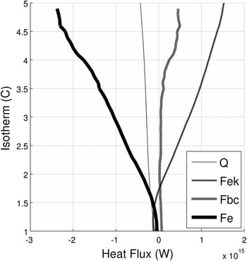
The results are strongly dependent on the choice of the isotherm used for the heat flux integration (Fig. 2). While de Szoeke & Levine (Reference De Szoeke and Levine1981) used the 1.3°C, the 2.6°C isotherm is chosen here for the better representation of the region of high potential temperature gradient corresponding to the Polar Front. When considering the 1.3°C isotherm to define the Polar Front, as used in de Szoeke & Levine (Reference De Szoeke and Levine1981), an eddy heat flux of -74 x 1013 W is obtained. This value is still ∼ 67% higher than the previous estimate. It is questionable, however, to use such an isotherm to represent the Polar Front in the Argo climatology, since it is located completely outside the zone of the maximum mean potential temperature gradient.
Heat balance terms as function of the isotherm used to represent the path of integration. The eddy component (Fe) is calculated as the resultant flux necessary to balance the other terms.

In Fig. 2, the distribution of the terms of the heat balance equation (Eq. (1)) as function of the isotherm used for its integration shows the dominance of the Ekman component (Fek) for most isotherm values. Only south of the 2.1°C isotherm (lower temperatures), the heat lost to the atmosphere (Q) dominates the balance. The change of direction of Fek from negative (southward) to positive (northward) at the 1.8°C isotherm reflects the transition to the region under the influence of the westerly winds. This indicates that surface buoyancy fluxes may dominate south of the ACC, while in the current core vicinity the balance is achieved mainly between the Ekman and the eddy terms.
This dominance of the Ekman component is important for the difference between the present eddy heat flux and the results of de Szoeke & Levine (Reference De Szoeke and Levine1981). While these authors estimated an Ekman layer heat flux of 15 x 1013 W, the present results shows considerably higher values (49 x 1013 W for the 2.6°C isotherm - the Polar Front; and -12 x 1013 W for the 1.3°C isotherm - the value used by de Szoeke & Levine Reference De Szoeke and Levine1981). The higher value of the Ekman contribution to the balance can be explained by the intensification and southward migration of the westerly winds.
Several authors, such as Meredith & Hogg (Reference Meredith and Hogg2006), related an increase in the eddy heat flux across the SO to the observed southward migration of the westerly winds. This phenomenon is captured by the present analysis, since the data used in this study encompass the years 2006–09, more than 25 years later than the data used by de Szoeke & Levine (Reference De Szoeke and Levine1981). As an example, according to Fyfe et al. (Reference Fyfe, Saenko, Zickfeld, Eby and Weaver2007) the IPCC AR4 models estimate an approximate 25% strength increase and 3.5° latitudinal shift in the annual mean wind stress maximum from 1850–2100. While this estimate gives a general idea of the increasing wind stress over the SO, recent measurements show that such intensification is itself variable in time, being stronger in recent years. As an example Luis & Pandey (Reference Luis and Pandey2004), using scatterometer data, observed a 40% difference in the winter wind stress over the SO between the years of 2000 and 2003.
A direct link between the wind induced heat flux and the MOC in the SO was described by Abernathey et al. (Reference Abernathey, Marshall and Ferreira2011), which is dependent on both the wind stress and the surface boundary condition for buoyancy. Since a realistic surface heat flux was used in the balance (ERA-Interim reanalysis), this effect is captured in the presented results.
Since the Ekman layer heat flux is calculated across a circumpolar path, it assumes a deep return flow to assure the volume conservation of the southern seas. Although reasonable when dealing with a climatological circumpolar path, this volume balance should not hold locally. In fact, deep currents are expected to play an important role in specific regions, such as the eastern limit of the Weddell Sea, the South Sandwich Islands and the Kerguelen Plateau (e.g. Fukamachi et al. Reference Fukamachi, Rintoul, Church, Aoki, Sokolov, Rosenberg and Wakatsuchi2010). Consequently the results of the proposed heat balance should be taken only in its integral form.
Quantifying the errors involved in the Ekman term of the heat balance equation (Eq. (1)) is a complicated task since the uncertainty in the wind stress reanalysis field is not available. However, taking into account that the ERA-Interim reanalysis is generated with the assimilation of scatterometer data (Dee et al. 2011), the mean deviations of this dataset can be used as a proxy to calculate an estimate of the error. An estimation of this value is provided by Chelton & Freilich (Reference Chelton and Freilich2005). They observed a mean 1.3 m s-1 difference between the QuickSCAT scatterometer winds and buoy measurements in the North Atlantic and Pacific oceans. Considering this value as a first guess for the SO uncertainties (no local estimates are available), and using the standard deviation of the T and S climatologies for the ocean structure, an error of ± 16.25 x 10¹³ W in the Fek is obtained.
According to de Szoeke & Levine (Reference De Szoeke and Levine1981), the contribution of the geostrophic baroclinic flow is very small when compared to the Ekman layer and ocean-atmosphere heat fluxes, although these authors did not access its geographical distribution. Using the 2.6°C isotherm as a reference (Fig. 3), it is possible to observe that regions with higher geostrophic baroclinic heat flux coincide with deflections in the Polar Front path, showing that some contamination from the mean flow may be present. Similarly, the Ekman layer heat flux (always northward) is more intense at low latitudes of the Polar Front, evidencing the stronger influence of the westerly wind corridor.
Ekman layer (blue) and geostrophic baroclinic (red) contributions to the heat balance across the Polar Front.

Using the standard deviation of the individual Argo T and S profiles in relation to the climatology in the Fbc equations presented by de Szoeke & Levine (Reference De Szoeke and Levine1981), it is possible to estimate the expected error in the baroclinic contribution term of the balance equation, Eq. (1). An error of 0.19 x 10¹³ W is obtained for the integrated baroclinic heat flux across the Polar Front, which is small when compared to the total values of the balance terms.
Since de Szoeke & Levine (Reference De Szoeke and Levine1981) did not present error bars for all the terms involved in the balance, the comparison between their estimates and ours is compromised. Although the present results suggest a higher total heat flux across the Polar Front, possibly all that can be asserted with confidence is that both values are of the same order. Moreover, the new dataset confirms the eddy heat flux as the dominant component to balance the Ekman heat transport. Errors involved in the computation of the surface heat loss to the atmosphere (Q) could not be calculated and may significantly contribute to the result uncertainty. However, a first order estimate of the uncertainty involved in the present calculations can be obtained by adding the baroclinic and Ekman layer component errors of the balance equation, Eq. (1), resulting in a total of ± 16.45 x 10¹³ W uncertainty in the heat balance results. It is important to emphasize that this is a lower bound estimate, since part of the uncertainty could not be accounted for.
Parametric model
The balance equation gives an indirect estimate of the eddy component (Fe). Although a circumpolar direct calculation cannot be performed with the available in situ data, it can be reached by means of a parameterization.
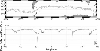
Using the parametric model described in the Methods section to obtain a direct estimation of the eddy heat flux across the Polar Front, an annual mean value of -56.2 x 10¹³ W was calculated. This value is in the range established by previous observational studies (Table I) and in the order of the results provided by numerical simulations (∼10–30 x 1013 W) performed by Farneti & Delworth (Reference Farneti and Delworth2010), but lower than the results based on the heat balance. The best comparison is obtained with the fluxes derived from current meter data, although present series are still too short to obtain statistically representative results. Moreover, the extrapolation of punctual observations to the circumpolar ACC is not straightforward due to the large geographical variation of the fluxes (Fig. 4).
a. Mean position of the Polar Front obtained from the monthly gridded Argo product, and its northern and southern maximum positions between January 2005 and December 2009. b. Geographical distribution of the mean eddy heat flux (W m-1) obtained by the parameterization for the 48 months of the present study.

The eddy temperature flux can be very important in local terms, as described by Meijers et al. (Reference Meijers, Bindoff and Roberts2007). Large values are concentrated in a few narrow regions: the Pacific-Antarctic ridge (∼140°W), the western Atlantic (after the Drake Passage, at ∼50°W), south of the Agulhas Current retroflection (∼20–30°E), east of the Kerguelen Plateau (∼85°E), and the Campbell Plateau (∼150°E). Such regions are related to deflections in the Polar Front orientation and/or the presence of topographic barriers in the main ACC current path (see Fig. 4a).
The largest heat flux is observed in the Atlantic sector, close to the Weddell Sea (Fig. 4b). This is particularly important since this is the region where almost half of the total volume of the Antarctic Bottom Water (AABW) is formed (Fahrbach et al. Reference Fahrbach, Hoppema, Rohart, Boebel, Klatt and Wisotzki2011). Anomalies in the meridional heat flux will have an impact on the heat content of the Weddell Sea and hence on the water column density structure. Stössel & Kim (Reference Stössel and Kim2001), for instance, related the variability in the formation of AABW to the amount of North Atlantic Deep Water (NADW) that enters the Weddell Sea, in the form of Lower Circumpolar Deep Water (LCDW). Since this water mass presents relatively high temperatures, it can be associated to the high southward eddy heat flux in this region. The results from the parametric model indicate that the mesoscale activity is an important process associated with these high values of heat flux.
Meijers et al. (Reference Meijers, Bindoff and Roberts2007) discussed the contribution of individual eddies to the heat flux in an eddy permitting numerical simulation. The authors proposed that large eddies may have an important local contribution while small eddies that are not resolved in the current optimally interpolated SLA products may be important in a circumpolar point of view. This is important when considering the effect of individual structures on the eddy heat flux. In fact, several rings have been observed to cross the Polar Front in the regions of high fluxes west of the Drake Passage and south of Africa in the SLA data. This indicates that large eddies are important in regions of intense fluxes, although a direct calculation would be necessary in order to quantify their influence. Other processes contribute to the eddy heat flux as well. Beyond the rings studied by Meijers et al. (Reference Meijers, Bindoff and Roberts2007), Hughes (Reference Hughes1996) characterized the ACC as a wave guide of Rossby waves, and Ciasto & Thompson (Reference Ciasto and Thompson2008) related fluctuations of the current field on timescales close to ten days to the effect of high frequency wind stress variability, both of which contribute to the eddy heat flux across the front.
Since the parametric model relies on the mixing length theory (Holloway Reference Holloway1986, Ferrari & Nikurashin Reference Ferrari and Nikurashin2010), the eddy diffusivity is linked to the geostrophic turbulence spectrum tilt including different length scales responsible for the heat flux. This is a common assumption used to represent the eddy mixing in climate models, i.e. that the eddy tracer fluxes are related to the mean tracer gradients through an eddy diffusivity proportional to the r.m.s. eddy velocity and a mixing length. As shown by Ferrari & Nikurashin (Reference Ferrari and Nikurashin2010), this is a good approximation for the eddy fluxes, although some modification of the mixing length calculation may be necessary when considering the mean flow influence. Such modification should account for the suppression of the meridional eddy flux by strong zonal fluxes in the ACC core.
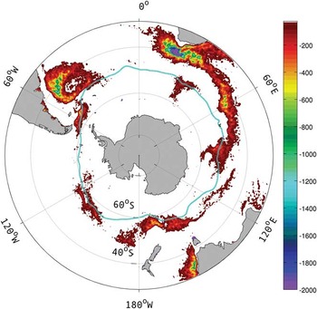
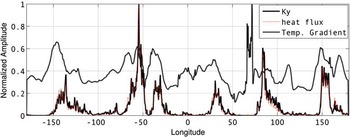
In Fig. 5, it is possible to observe the coincidence of high meridional eddy diffusivities (Ky) with the high eddy heat flux regions presented in Fig. 4b, evidencing the problem of extrapolating local measurements to obtain circumpolar estimates of the eddy heat flux. This factor possibly accounts for the high values of eddy heat flux obtained by Phillips & Rintoul (Reference Phillips and Rintoul2000). Indeed, the values of Ky presented in Fig. 5 have the same order of magnitude as the theoretical predictions for the Pacific sector of the SO obtained by Ferrari & Nikurashin (Reference Ferrari and Nikurashin2010) and are slightly higher than the vertical integral of the “effective diffusion” obtained by Abernathey et al. (Reference Abernathey, Marshall and Mazloff2010) when using tracer distribution from an advection-diffusion model. The longitudinal distribution of the parameterization terms in Fig. 6 shows a remarkable coincidence between the eddy heat flux and Ky. This shows that Ky has a dominant influence over the calculated heat flux, presenting a 85% correlation factor, while the correlation between the heat flux and the temperature gradient is 22%.
Meridional eddy diffusivity (m2 s-1) calculated from the parameterization. Values lower than 50 m2 s-1 were excluded for a clear visualization of the regions of larger contribution. The blue line indicates the mean position of the Polar Front obtained from the Argo climatology, coincident with the vertical mean 2.6°C isotherm.

Normalized amplitudes of the temperature gradient, eddy diffusion coefficient (Ky) and parameterization derived eddy heat flux. This value corresponds to the mean of the study period (2006–09).

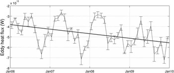
Similarly to the baroclinic contribution to the heat balance, the standard deviation of the individual T and S profiles from the monthly climatologies was used to calculate the expected error in the parameterization results. These monthly errors are presented as vertical bars in Fig. 7 and have a mean value of ± 0.35 x 10¹³ W. Accumulating the monthly errors along each year and averaging over the four years used in the present analysis results in a mean error of ± 4.18 x 10¹³ W in the annual mean eddy heat flux obtained by the parameterization.
Temporal variability of the integrated eddy heat flux across the Polar Front, obtained from the parameterization, with the error bars derived from the standard deviation of the Argo profiles in relation to the monthly T and S mean fields. A linear fit shows the increase of the southward eddy heat flux between the years of 2006 and 2009, with a mean trend of -0.44 x 10¹³ W year-1.

Since the SLA dataset errors, that directly influence the Ky, were not considered in the eddy heat flux error calculations, the obtained uncertainty should be considered as a lower bound estimate. Although this may contribute to the observed difference between the parametrization and balance equation uncertainties, the direct approach and lower number of error sources (terms in Eq. (1)) also impact the smaller parameterization uncertainty.
Heat flux variability
Despite the short period of time of the SLA data used (2006–09), the interannual variability of the eddy heat flux computed through the parameterization can be analysed. Applying the Holloway (Reference Holloway1986) parameterization to monthly mean SLA and Polar Front positions, it was possible to obtain monthly values for the eddy heat flux across the Polar Front in the study period (Fig. 7).
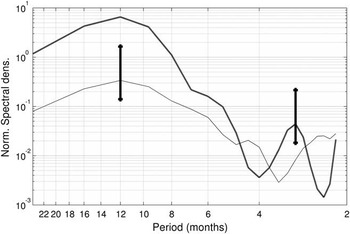
The seasonal cycle is dominant in the eddy heat flux spectrum in Fig. 8, with a mean amplitude of 0.75 x 10¹³ W. Although this value is small when contrasted to the annual eddy heat flux error presented in the previous section (±4.18 x 10¹³ W), it is important in comparison to the monthly errors (±0.35 x 10¹³ W). The spectrum was calculated from the detrended eddy heat flux time series, low pass filtered using a Hanning window with a seven months cut-off period.
Normalized temporal spectra of the eddy heat flux across the Polar Front (solid line) obtained from the parameterization and the first empirical orthogonal function of the meridional position of the Polar Front (dashed line). The vertical lines show the 95% confidence interval. A five months Hanning window was applied to the spectra.

Due to the short time span of the SLA data, the low frequency (interannual) variability is underrepresented. However, analysing the unfiltered eddy heat flux obtained from the parameterization, a robust tendency of increasing southward eddy heat flux is observed. An increasing trend of 0.44 x 10¹³ W year-1 for the southward eddy heat flux can be observed (dashed line in Fig. 7), comparable with the seasonal variability signal. Although this value is small when compared to the annual mean error for the parameterization results, it is consistent along the four years analysed. It can be observed in Fig. 7 that both the seasonal variability and the interannual trend are robust when compared to the monthly error bars. This trend of increase in the eddy heat flux can be related to the increasing SO heat content obtained by Meijers et al. (Reference Meijers, Bindoff and Rintoul2011) using an empirical mode mapping based on historical hydrographic and satellite data. The authors estimated an increase of 1.196 ± 0.090 W m-2 in the heat content of the SO in 18 years (1992–2010), distributed over most of its extent and at all depths. Integrating this value over the ocean south of the Polar Front results in an annual increase of 0.22 x 10¹³ W in the heat content. Although smaller, this value is in the same order of the increasing heat flux obtained by the present study. This difference may be explained by two facts: 1) the results from Meijers et al. (Reference Meijers, Bindoff and Rintoul2011) refer to the heat content of the whole SO, while the present work focuses on the Polar Front where a higher variation is expected, and 2) their results are constrained by the 2000 m depth limit of the datasets used, while the heat flux in the present study is integrated over the full depth in the Polar Front path (∼4000 m).
The observed increase in the eddy heat flux has important impacts on the MOC. As an example, Purkey & Johnson (Reference Purkey and Johnson2010) observed basin wide warming of the AABW between the 1980s and 2000s related to the warming of the Warm Deep Water (WDW) in the Weddell Sea, one of its main source waters. This process is directly influenced by the heat flux entering the Weddell Sea in the Atlantic sector of the SO. In recent studies, high-resolution model results (e.g. Screen et al. Reference Screen, Gillet, Stevens, Marshall and Roscoe2009) indicate little changes in the mean overturning as consequence of the increasing southward eddy fluxes. On the other hand, coarse resolution models that do not explicitly resolve the eddy activity suggest an increase of the subpolar upwelling cell, with a consequent increase in the upwelling of deep carbon rich Upper Circumpolar Deep Waters (UCDW) south of the ACC (Saenko et al. Reference Saenko, Fyfe and England2005). Since in the present study the mean potential temperature of the Polar Front is held constant in the calculation of the eddy heat flux, the results should be interpreted as an intensification in the cross-frontal circulation.
Several recent studies (e.g. Fyfe et al. Reference Fyfe, Saenko, Zickfeld, Eby and Weaver2007, Screen et al. Reference Screen, Gillet, Stevens, Marshall and Roscoe2009) related the strengthening and southward shifting of the westerly winds to the augmenting southward heat flux and consequent subsurface warming in the SO. Gille (Reference Gille2008) associated most (87%) of the observed SO warming to the southward shifting of the ACC fronts. In fact, the observed modification in the seawater properties of the SO (e.g. Böning et al. Reference Böning, Dispert, Visbeck, Rintoul and Schwarzkopf2008) are consistent with a southward migration of the isopycnal surfaces by about 50 km. Since the present calculations were made in relation to time varying fronts defined by vertical mean isotherms, the observed trend in the eddy heat flux expresses a real cross-frontal warming tendency.
Such meridional migration was not observed for the Polar Front position obtained from the 2.6°C isotherm due to the short period of time analysed. Moreover, it is interesting to note that the seasonal cycle dominates the spectrum of the temporal component of the first empirical orthogonal function (EOF) of the meridional position of the Polar Front (which explains 55% of the total variance) (Fig. 8). A three months period variability is also observed, although in the limit resolved by the monthly mean data. Barotropic Rossby waves propagating in the Polar Front (Hughes et al. Reference Hughes, Meredith and Heywood1999) or the ocean-atmosphere interactions associated with the Southern Hemisphere Annular Mode (SAM) (Meredith et al. Reference Meredith, Woodworth, Hughes and Stepanov2004) are possibly connected to higher frequency processes. In fact, a 20% correlation is observed between the SAM index and the mean meridional position of the Polar Front, filtered to remove the influence of the seasonal cycle. Such a low correlation indicates this process does not play a dominant role in the observed Polar Front position.
Kerr et al. (Reference Kerr, Mata and Garcia2009) suggested a link between the SAM and the Weddell Sea Bottom Water, but the same is not observed for the obtained eddy heat flux, since a very low correlation was obtained between the total eddy heat flux across the Polar Front and the SAM index (∼2%). This is a consequence of: 1) the filter of high frequency variability, and 2) the use of a variable Polar Front position. Such influence is evidenced by the absence of short period energy peaks in the heat flux spectrum of Fig. 8.
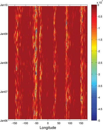
Despite the observed trend in the eddy heat flux, the regions of higher concentration identified in Fig. 4 are still constant in time. The Hovmoller diagram in Fig. 9 shows that, even though a high temporal variability is present, the spatial distribution of the heat flux does not change during the analysed period. Indeed, although the EOF of the eddy heat flux does not show a robust dominant mode (the first EOF correspond to ∼12% the total variance), combining the first five modes yields 39% of the variance and follow the same spatial pattern shown by the mean eddy heat flux. No propagating pattern is observed in the Hovmoller, since the heat flux was calculated in relation to monthly Polar Front positions. This means that large period waves, such as the barotropic circumpolar waves described by Hughes et al. (Reference Hughes, Meredith and Heywood1999), were filtered in the analysis and have no influence on the results.
Hovmoller diagram of the eddy heat flux (W m-1) across the Polar Front obtained from the parametric model. The regions of higher southward eddy heat flux are constant with time, varying only in amplitude.

Conclusion
Two methods were applied in order to estimate the eddy heat flux across the Polar Front: a heat balance, and a parameterization based on SLA data. While the first method is an indirect estimate, attractive by its simplicity, the parameterization is a direct estimate providing the geographical distribution of the eddy heat flux and its temporal variability during the study period (2006–09). Both methods independently confirm the dominant role of the mesoscale eddy heat flux on the heat balance in the SO.
The heat balance, based on the ideas of de Szoeke & Levine (Reference De Szoeke and Levine1981), presented a resultant eddy heat flux (-80.5 ± 16.45 x 10¹³W) in the range established by previous works (de Szoeke & Levine Reference De Szoeke and Levine1981, Stammer Reference Stammer1998, Phillips & Rintoul Reference Phillips and Rintoul2000, Sloyan & Ritoul 2000) (see Table I). This analysis indicates that other processes besides mean geostrophic currents and wind drift should be important in the southward heat flux through the Polar Front. From the results of the parameterization, we reinforce that eddy fluxes should provide such transport.
The geographical distribution obtained from the parameterization shows a pattern of concentrated regions of eddy heat flux, unchanging through the analysed period. An important contribution is observed in the portion of the SO adjacent to the South Atlantic, potentially influencing important deep and bottom water formation sites.
The eddy diffusivity coefficient (Ky) computed with the parametric model compares well with modern results (Ferrari & Nikurashin Reference Ferrari and Nikurashin2010, Abernathey et al. Reference Abernathey, Marshall and Mazloff2010). The resultant mean eddy heat flux (-56.2 ± 4.18 x 10¹³ W) is consistent with published results (Table I), although smaller than the value obtained from the heat balance. A consistent trend of increasing southward eddy heat flux was obtained with the parametric model applied to monthly values (-0.44 x 10¹³ W year-1). This trend is compatible with recent numerical simulation results (Farneti & Delworth Reference Farneti and Delworth2010) and observations (Meijers et al. Reference Meijers, Bindoff and Rintoul2011).
The uncertainty assessment for the two methods’ results are not similar, since distinct error sources are considered. However, the fact the parameterization provides a direct estimate of the eddy heat flux, derived from a large dataset that covers the whole Polar Front region during the study period, contributes to the lower uncertainty and larger reliability of this method.
Despite the agreement in terms of the order of magnitude of the eddy heat flux between the present and previous studies, we still lack knowledge regarding its vertical distribution. In fact, Meijers et al. (Reference Meijers, Bindoff and Roberts2007) cited as the most important unresolved aspects of the eddy fluxes in the SO: the spatial distribution, depth range, and degree of significance outside the ACC. This paper contributes to clarify the first one.
Numerical model results can be used to understand the influence of the mesoscale variability over the vertical frontal structure observed in the SO. Nowadays, several eddy resolving models are available for the scientific community, although most climate models to this date present coarse resolution in their oceanic components. The results obtained by such models diverge from the results obtained by the eddy resolving simulations regarding the modifications in the SO MOC in recent years. Further analyses are necessary to understand the mechanisms connecting the observed atmospheric changes and the MOC variability, improving the confidence in future climate change scenarios.
Acknowledgements
The present work would not be possible without the support from the Coordenação de Aperfeiçoamento de Pessoal de Nível Superior (CAPES) and the Institute Français de Recherche pour l'Exploitation de la Mer (IFREMER). Special thanks to all the crew of the Coastal and Oceanographic Engineering Group, from the Program of Ocean Engineering (PenO) of COPPE/UFRJ, and in particular to the Oceanic Processes Laboratory. Thanks to Marcia Hsu for the text revision. The authors would also like to acknowledge the two anonymous reviewers for their valuable contributions to improve this manuscript.