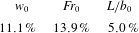
1 Introduction
Line fountains arise when dense fluid is projected vertically upwards into a less dense environment under release conditions that are two-dimensional at the source. In the laboratory setting, such release conditions are approximated by discharging fluid uniformly through long and thin rectangular ‘slot’ sources made in a horizontal plane. Thus, for a slot of length
 $L$
and half-width
 $b_{0}$
, the fountains of interest are those formed if the source aspect ratio
 $L/b_{0}\gg 1$
. Herein, we follow the consensus in the literature by referring to these high-source-aspect-ratio releases as ‘line fountains’, although we acknowledge that they are not true lines in the mathematical sense. A Cartesian coordinate system is adopted, centred on the midpoint of the source, with
 $x$
the spanwise,
 $y$
the cross-stream and
 $z$
the streamwise coordinate. Views onto the
 $(x{-}y)$
plane are designated as ‘top views’, onto the
 $(y{-}z)$
plane as ‘end views’ and onto the
 $(x{-}z)$
plane as ‘side views’. The slot therefore spans
 $x\in [-L/2,L/2]$
(spanwise) and
 $y\in [-b_{0},b_{0}]$
(cross-stream). Our focus herein lies exclusively on free turbulent fountains produced by miscible fluids with density differences sufficiently small that the flow may be regarded as Boussinesq. As we shall see (§ 3), the interaction with the upflowing jet with dense fluid structures collapsing under gravity from the fountain top resulted in a turbulent fountain, even at relatively modest source Reynolds number
 $Re_{0}$
. Indeed, the turbulent nature of the fountain was evident both based on viewing the flow externally and on viewing the internal flow – for the latter, the upflowing jet was always observed to expand in response to the turbulent entrainment of the surrounding fluid.
Fountains issuing from high-aspect-ratio rectangular sources have been studied experimentally by Zhang & Baddour (Reference Zhang and Baddour1997) and Srinarayana et al. (Reference Srinarayana, Williamson, Armfield and Lin2010). Experiments have also been conducted on linear arrays of closely spaced circular sources as approximations to such high-aspect-ratio rectangular sources (Baines, Turner & Campbell Reference Baines, Turner and Campbell1990; Bloomfield & Kerr Reference Bloomfield and Kerr1998). Momentum-rich releases give rise to so-called ‘forced’ fountains, and the picture that emerges from these experiments is that of a negatively buoyant jet-like core extending upwards from the source and shedding dense lobes of fluid to either side of the core – the descending fluid being referred to as the counterflow. Reports concerning the quasi-steady, i.e. established, behaviour differ, some claiming that the flow ‘flaps’ laterally about the source (Zhang & Baddour Reference Zhang and Baddour1997; Srinarayana et al. Reference Srinarayana, Williamson, Armfield and Lin2010), whilst others argue that the flow retains a symmetric structure punctuated by prolonged asymmetric transients (Baines et al. Reference Baines, Turner and Campbell1990).
Viewed from one end, experimentalists nevertheless broadly agree that the time-averaged established vertical height of rise follows
 $$\begin{eqnarray}\overline{z}_{v}=C\,b_{0}Fr_{0}^{4/3}\quad \text{for}~Fr_{0}\gtrsim 6.5,\quad Fr_{0}\equiv \frac{w_{0}}{\sqrt{b_{0}\,g_{0}^{\prime }}},\end{eqnarray}$$
with the pre-factor
 $C$
measured between
 $1.64$
(Baines et al.
Reference Baines, Turner and Campbell1990, corrected; the original publication mistakenly quoted
 $C=0.63$
, see Hunt & Coffey Reference Hunt and Coffey2009) and
 $2.00$
(Zhang & Baddour Reference Zhang and Baddour1997). In (1.1),
 $Fr_{0}$
denotes the source Froude number,
 $w_{0}$
the mean vertical velocity at the source and
 $g_{0}^{\prime }$
the reduced gravity of the source fluid. A summary of previous measurements of forced line fountains is presented in table 1. By contrast, at lower Froude numbers, relatively momentum-poor releases produce ‘weak’ fountains that display a variety of behaviours depending on the values of
 $Fr_{0}$
and
 $Re_{0}\equiv w_{0}b_{0}/\unicode[STIX]{x1D708}_{0}$
, with
 $\unicode[STIX]{x1D708}_{0}$
the kinematic viscosity of the source fluid (Srinarayana et al.
Reference Srinarayana, Williamson, Armfield and Lin2010). Stratifying the environment has been shown to reduce the rise height (Bloomfield & Kerr Reference Bloomfield and Kerr1998) and to delay the onset of instabilities (Inam et al.
Reference Inam, Lin, Armfield and He2015).
Summary of release conditions and measurements for forced turbulent line fountains. BTC90 refers to Baines et al. (Reference Baines, Turner and Campbell1990); Z&B97 to Zhang & Baddour (Reference Zhang and Baddour1997); HDC19 to this study where data from § 4 are included. RS denotes rectangular slot and PT denotes perforated tube. Baines et al.’s (Reference Baines, Turner and Campbell1990) estimate of
 $L/b_{0}$
is based on a virtual origin correction. *Value based on a fit to the pooled data for the three aspect ratios listed. An entry for Srinarayana et al. (Reference Srinarayana, Williamson, Armfield and Lin2010) is not included as therein the fountains were not at sufficiently high
 $Fr_{0}$
to be considered as ‘forced’. The definition of the time- and spanwise-averaged rise height
 $\overline{\overline{z}}_{v}$
is given in § 4.2;
 $\unicode[STIX]{x1D6FE}_{z}$
is the constant of proportionality for the associated rise height scaling.

Free-shear flows from rectangular sources have also been studied for the cases of a line jet (Krothapalli, Baganoff & Karamcheti Reference Krothapalli, Baganoff and Karamcheti1981; Deo, Mi & Nathan Reference Deo, Mi and Nathan2008; Paillat & Kaminski Reference Paillat and Kaminski2014) and a line plume (Kotsovinos & List Reference Kotsovinos and List1977). Indeed, prior to the development of a counterflow, one would expect the initial near-field development of a line fountain to share similarities with a starting line jet. Krothapalli et al. (Reference Krothapalli, Baganoff and Karamcheti1981) examined the jet that issued from a rectangular slot and noted that at distances from the origin comparable to approximately three slot lengths, the jet transitioned to a behaviour analogous to the round jet, thereby ‘losing’ information about the source. Herein, our observations are restricted to fountains whose time- and spanwise-averaged rise height is less than the length of the slot (
 $\overline{\overline{z}}_{v}/L<1$
) and as such, whose source geometry retains its influence on the structure of the fountain.
The rise height (1.1) and, indeed, all observations reported previously stem from experiments conducted in visualisation tanks of spanwise dimension equal to the length
 $L$
of the slot. Side walls at
 $x=\pm L/2$
thereby bounded the source and restricted the fountain to a length
 $L$
. It is implied, for lack of commentary otherwise, that these experimental conditions resulted in a flow that behaved uniformly along the spanwise dimension (
 $x$
). Consequently, the flow was inspected only as viewed from one end (
 $y{-}z$
). Theoretical modellers followed suit: drawing from experimental evidence, line fountains were treated as uniform along
 $x$
and the conservation equations associated with the integral modelling of a round fountain were recast in terms of fluxes per unit length. Analytical solutions were developed that successfully predict the initial rise of Boussinesq (Hunt & Coffey Reference Hunt and Coffey2009) and non-Boussinesq (van den Bremer & Hunt Reference van den Bremer and Hunt2014b
) line fountains in a homogeneous environment, whilst numerical solutions additionally account for background stratification (Bloomfield & Kerr Reference Bloomfield and Kerr1998). However, as yet there is no mathematical model for predicting the quasi-steady state behaviour of turbulent line fountains, a state in which there are turbulent exchanges and an interplay between the upflowing core and descending counterflow. Herein, our observations and measurements of the fountain as a whole establish why a straightforward extension of the integral modelling approaches that have proven so successful for round fountains (see the review of Hunt & Burridge Reference Hunt and Burridge2015) will fail to capture the general behaviour of quasi-steady line fountains.
Real sources are of finite length and end effects propagating inwards (such as boundary layers growing along the side walls of the aforementioned visualisation tanks) limit the applicability of two-dimensional theory to a central section of the flow, although the extent of this limitation has not previously been explored. Moreover, the assumption of uniformity along the span has led experimentalists (Baines et al.
Reference Baines, Turner and Campbell1990; Zhang & Baddour Reference Zhang and Baddour1997; Bloomfield & Kerr Reference Bloomfield and Kerr1998; Srinarayana et al.
Reference Srinarayana, Williamson, Armfield and Lin2010) to analyse fountain behaviour exclusively in the (
 $y{-}z$
) plane, that is, as viewed from the end of the slot. This single view neglects to account for any possible spanwise variation. As a result, prior to this investigation little was known about the physical structure of the flow in three dimensions other than, as exemplified by the numerical simulations at
 $Fr_{0}=10$
(Inam et al.
Reference Inam, Lin, Armfield and He2015), it is complex and markedly non-uniform along the span.
There is therefore clear scope for developing an understanding of line fountains by studying their structure and dynamics in three dimensions. To this end, we performed and report on experiments with aqueous-saline fountains that are distinct from previous research in the following important ways. Our line fountains were: (i) formed from slots whose ends were free, i.e. far from adjacent walls; (ii) formed from slots of aspect ratio far exceeding those of existing experiments (see table 1 for details); and (iii) interrogated simultaneously from the top and side. Additionally, (iv) the internal structure of these fountains was studied in a vertical section cutting across the centre of the slot. This internal view proved crucial to understanding the interaction of the upflowing core with the counterflowing regions. The insights into line fountain behaviour afforded by these multiple views, coupled with the quantitative measurements we have made of their spatial and temporal variations, provide a guide for the future development and validation of predictive models of their quasi-steady dynamics. Prior to the current study, the mean vertical rise height (1.1) was the only statistic reported.
The remainder of this paper is structured as follows. We proceed by describing the experimental set-up in § 2. The fountain is then analysed qualitatively in § 3 through synchronous top and side visualisations which confirm that the behaviour is, in general, not uniform along the span. The insights gained by dye-attenuation measurements are reinforced through fluorescence visualisations of the internal structure which reveal the mechanism underlying the primary non-uniformity. By combining the results of diagnostics applied separately to the top and side views, we show how the local rise height variations are related to a global, lateral (side-to-side) swaying of the fountain. Thereby, we identify in § 4 a main driver for shaping the structure of line fountains. Conclusions are drawn in § 5.
2 Experimental procedure
2.1 General arrangement
Experiments were conducted in a water-filled visualisation tank of dimensions 0.7 m (height)
 $\times$
1.0 m
 $^{2}$
(base) made of clear acrylic. A nozzle, positioned centrally on the base, steadily released a saline solution (NaCl) vertically upwards through a slot of length
 $L=\{300,150\}$
mm and half-width
 $b_{0}=0.5$
mm. The source aspect ratios were thus
 $L/b_{0}=\{600,300\}$
. Precautions were taken to ensure that the release conditions were uniform so that, as confirmed in §§ 3 and 4, the flow might reasonably be regarded as two-dimensional at the source. A detailed account of our bespoke nozzle design is given in appendix A. Notably in our arrangement, since the nozzle was positioned far from adjacent walls, the fountain produced was free to propagate in all directions.
Saline solution was delivered to the nozzle by means of a high-precision gear pump: an Ismatec MCP-Z Process at low to moderate flow rates, and a Pompe Cucchi HCX41 at high flow rates. These pumps were connected to an Atrato ultrasonic flow meter which logged the trace of the source volume flow rate
 $Q_{0}$
during experiments. This trace allowed us to verify that
 $Q_{0}$
was satisfactorily constant, with standard deviations within
 $1\,\%$
of the base flow rate. The density of the saline solution
 $\unicode[STIX]{x1D70C}_{0}$
and environment
 $\unicode[STIX]{x1D70C}_{a}$
were measured with an Anton Paar DMA5000 densitometer to within an accuracy of
 $5\times 10^{-5}~\text{g}~\text{cm}^{-3}$
. Densities ranged from
 $\unicode[STIX]{x1D70C}_{0}=1.0001$
to
 $1.0210~\text{g}~\text{cm}^{-3}$
, i.e.
 $(\unicode[STIX]{x1D70C}_{0}-\unicode[STIX]{x1D70C}_{a})/\unicode[STIX]{x1D70C}_{a}=1.4\times 10^{-3}$
to
 $0.022$
, well within the recommended range for Boussinesq flows (Mehaddi, Vauquelin & Candelier Reference Mehaddi, Vauquelin and Candelier2015). The range of experimental parameters we investigated is summarised in table 2 together with our estimates of the associated errors. Additionally, we estimate that relative errors on our rise height and frequency measurements are within 2 %; see appendix B.
The range of experimental parameters covered in this study for measurement sets A and B. The vast majority of experiments were run for
 $Fr_{0}\geqslant 6.5$
, producing what may be regarded as ‘forced’ line fountains (1.1). The source reduced gravity is defined as
 $g_{0}^{\prime }=g(\unicode[STIX]{x1D70C}_{0}-\unicode[STIX]{x1D70C}_{a})/\unicode[STIX]{x1D70C}_{a}$
. The mean source velocity
 $w_{0}$
(used in the estimate of
 $Fr_{0}$
) was estimated as the ratio of the source volume flux to the source area,
 $w_{0}=Q_{0}/2b_{0}L$
. Errors on
 $Fr_{0}$
and
 $Re_{0}$
are upper-bound estimates (see appendix B).

To commence an experiment, a valve (blocking return flow from the nozzle and providing back-pressure for the flow meter) was opened and the flow rate of saline solution increased to the target value
 $Q_{0}$
. Recordings at
 $24$
frames per second (f.p.s.) were started once the fountain had reached a quasi-steady state and continued either until the flow had been captured for a sufficient number of characteristic time scales (see § 4.1), or until the saline layer, which accumulated at the base of the tank, deepened to the level of the flange into which the slot was set (figure 1). Crucially, our results, e.g. of rise height in figures 7 and 13, confirm that the flow was captured over a sufficiently long duration.
2.2 Flow visualisation
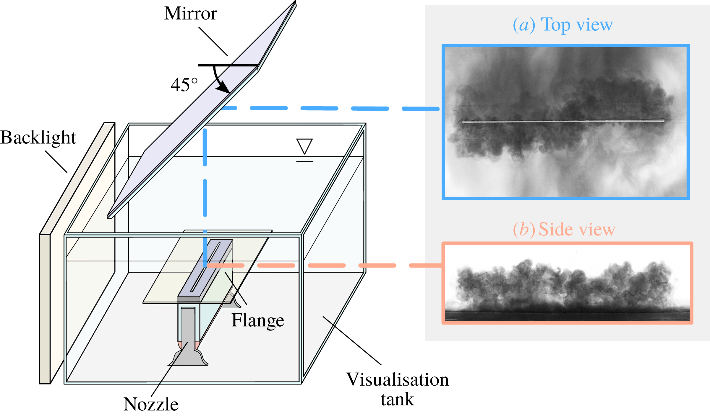
To aid flow visualisation, the source solution was stained with methylene blue and the flow uniformly backlit by an array of closely spaced high-frequency fluorescent tubes behind an opalescent screen. Two JAI Spark 5000-M CMOS cameras recorded the experiment: one, facing the long side of the nozzle, provided a side view (
 $x{-}z$
plane); the other, facing a plane mirror suspended above the tank at
 $45^{\circ }$
to the horizontal, provided a top view (
 $x{-}y$
plane). This arrangement is depicted in figure 1 with typical images of the fountain as viewed from these perspectives.
Schematic of the general experimental set-up. Cameras simultaneously recorded (a) the top view as seen through a
 $45^{\circ }$
mirror and (b) the side view. For the light-induced fluorescence experiments (§ 2.3) the backlight was replaced with a vertical light sheet.

Beyond lending a qualitative picture of the flow, dye visualisations are commonly coupled with edge detection techniques to extract quantitative information (e.g. Burridge & Hunt Reference Burridge and Hunt2013). In the side view (figure 1
b), the sharp contrast between the dyed fountain fluid and the clear ambient environment guaranteed the success of such techniques. In the top view (figure 1
a) however, contrasts are low as the dyed fountain fluid is set against approximately equally dyed gravity currents that laterally traverse the flange; thus, traditional edge detection failed. Even on applying alternative techniques, including edge-aware contrast enhancement, wavelet filtering, and partial differential equation based de-noising (Mathworks 2017), we found no reliable method for identifying the outline of the fountain in top views. Nevertheless, we show in § 3 that observing the spanwise motion from a top view is central to understanding fountain structure in three dimensions. Moreover, although the outline of the fountain viewed from above may not be traced accurately, the frequency of the lateral fluctuations (i.e. those in the
 $y$
-direction) can be confidently inferred from top views without relying on edge detection (§ 4.4). Analysing the flow in the
 $(y{-}z)$
plane provided a robust means of identifying the local outline.
2.3 Refractive index-matched light-induced fluorescence (LIF) visualisations
Flow visualisations were also conducted to study the fountain in the
 $(y{-}z)$
plane at a section cutting perpendicularly across the centre of the slot. In this case, the source solution was stained with fluorescein sodium and the internal structure of the fountain made visible by means of a vertical light sheet. A high-power (480 W) LED light strip Metaphase UL line light encased behind a 1 m vertical array of cylindrical lenses produced the light sheet. To improve beam quality, the edges of the beam were trimmed with a rectangular aperture slot before the beam entered the visualisation tank. This allowed for a
 $d=10$
mm thick light sheet with low divergence (spreading by 2 mm over a distance of 600 mm) so that
 $d/L\approx \{1/60,1/30\}$
.
Optical distortions, arising from differences in the refractive indices of saline and freshwater, prevented the clear visualisation of the flow in section due to the relatively lengthy (circa 200 mm) path of non-uniform saline concentration the fluoresced light rays travelled through. These distortions were most significant close to the source where the fountain upflow is bounded by laterally flowing currents. To minimise distortions, the density of the source solution was varied by adding sodium nitrate (NaNO
 $_{3}$
) salt and the environment by adding sodium chloride (NaCl) salt in such a way as to obtain different densities of solution with approximately equal refractive indices. The refractive indices of the chloride and nitrate solutions,
 and
 , were measured using a Hanna HI-96821 refractometer and matched to within
 .
3 Observations
In what follows, the three-dimensional fountain behaviours observed are described, first from the side, then from the top and finally in the central section. No clear dependence of the flow on
 $L/b_{0}$
was apparent in the side and end views, where the fountain’s height appeared to vary with
 $Fr_{0}$
only. By contrast, in the top views, where different lateral fluctuating patterns were observed, these varied with
 $L/b_{0}$
and
 $Fr_{0}$
. Most strikingly, the top views revealed that line fountains are generally not uniform in the spanwise direction.
3.1 Breakup of liquid sheet
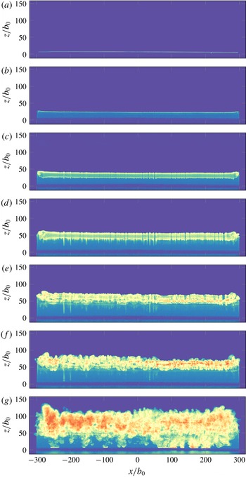
Initial transients were recorded for a few typical experiments at 60 fps in order to assess that the nozzle design achieved what may be regarded as uniform release conditions (figure 2). In figure 2(a,b), a uniform dense liquid sheet rises upwards from the source, with roll-up vortices forming symmetrically at either end of the slot. As the sheet rises further, a counterflow begins to form (seen as a bright horizontal band in figure 2 c,d) which descends around the upflow. Simultaneously, instabilities begin to appear along the span and grow into larger billows (figure 2 c,d), eventually leading to the turbulent breakdown of the flow (figure 2 e–g). Subsequently, the fountain adopts and maintains a quasi-steady structure. Significantly, images (a–g) provide convincing evidence for the uniformity of the release conditions. Further evidence is provided in § 4.1.
Whilst we were able to achieve a target value of
 $Fr_{0}$
after only a relatively short ‘ramp up’ time
 $t_{r}$
(achieving, at best,
 $t_{r}=0.1$
s), our rig was not designed to additionally explore the initial rise height. Exploratory observations we made indicated that evaluating the initial rise height is not as straightforward as it may seem given what has been previously reported. We observed that this height varies considerably depending on the impulsiveness of the injection that forms the fountain, i.e. with
 $t_{r}$
. The initial transients are therefore considered no further and the remainder of this article focuses on the quasi-steady structure.
The initial formation of a line fountain under near-impulsive start-up conditions from a slot of aspect ratio
 $600:1$
at
 $Fr_{0}=18.9$
highlighting the uniformity of the release conditions. Images (a–f), spaced
 $\unicode[STIX]{x0394}t=167$
ms apart, illustrate the breakdown of an initially laminar liquid sheet of dense fluid issuing vertically upwards from the source. The formation of the descending counterflow can clearly be seen from (c) onwards as a deepening horizontal band. Image (g), taken
 $60$
frames (i.e.
 $1$
s) after image (f), depicts the turbulent breakdown. Movie 1 available online (available at https://doi.org/10.1017/jfm.2019.514).

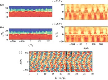
Synchronous side views (
 $z/b_{0}$
versus
 $x/b_{0}$
, instantaneous rise heights
 $z_{v}(x,t=\text{cst}.)$
superimposed as a black line) and top views (
 $y/b_{0}$
versus
 $x/b_{0}$
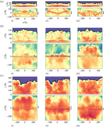
) showing: (a) non-uniform flapping; (b) uniform flapping; and (c) disorganised flapping. Top views show: for case (a) a non-uniform oscillation along the span in the form of a sinusoidal-like wave, with the central section out of phase with the ends (
 $y$
-scale magnified by a factor of two); for (b) that the fountain flaps uniformly along the span: ‘below’ (
 $y<0$
) the slot as seen in (i), then ‘above’ (
 $y>0$
) in (iii); and for (c) that whilst the flapping is uniform overall, the fountain top is dominated by large-scale structures which distort the regularity of this flapping. For (a)
 $\{L,b_{0}\}=\{300,0.5\}$
mm;
 $Fr_{0}=10.2$
(
 $Re_{0}\approx 53$
);
 $\unicode[STIX]{x0394}t=2.0$
s (
 $\cong 1.0~w_{0}/g_{0}^{\prime }$
); for (b):
 $\{L,b_{0}\}=\{150,0.5\}$
mm;
 $Fr_{0}=26.4$
(
 $Re_{0}\approx 114$
);
 $\unicode[STIX]{x0394}t=3.0$
s (
 $\cong 1.0~w_{0}/g_{0}^{\prime }$
); and for (c)
 $\{L,b_{0}\}=\{300,0.5\}$
mm;
 $Fr_{0}=51.3$
(
 $Re_{0}\approx 114$
);
 $\unicode[STIX]{x0394}t=7.5$
s (
 $\cong 2.0~w_{0}/g_{0}^{\prime }$
). Movies 2–4 available online.

3.2 Spatial structure and flapping patterns
Sample images of that quasi-steady structure are given in figure 3(a–c) in order to reveal the role of
 $Fr_{0}$
(and, to a lesser extent, of
 $L/b_{0}$
). Although our results herein may be regarded as
 $Re_{0}$
-independent, as reasoned in appendix C, the approximate value of
 $Re_{0}$
is given in the captions for completeness. The images shown were chosen specifically to highlight the distinct behaviours observed, behaviours we refer to as non-uniform flapping (figure 3
a), uniform flapping (figure 3
b) and disorganised flapping (figure 3
c) on account of the swaying (or flapping) motions of the fountain about a vertical plane through the source, hereafter referred to as the centre plane.
Judging first from the side views alone, the flow instantaneously resembles a wall of fluid with irregular wave-like crenellations formed by distinct turbulent structures, or eddies, that populate the fountain top. The motion of these structures, which extend in the vertical (
 $z$
) and spanwise (
 $x$
) directions, results in the localised vertical fluctuations. Neither the height of rise, nor the size of these structures appears to vary noticeably along the span for given release conditions. On increasing
 $Fr_{0}$
, the fountain rises to a greater height. The scale of structures at, or near, the fountain top also increases both in the vertical and spanwise directions. For example, at
 $Fr_{0}\approx 10$
(figure 3
a) one counts
 $O(20)$
structures over a length
 $L=600b_{0}$
(i.e. above the source), whereas at
 $Fr_{0}\approx 50$
(figure 3
c) one discerns only three to four structures over the same length. Thus, whilst the absolute size of large-scale structures increases with
 $Fr_{0}$
, the relative fraction of space they occupy along the span is evidently a function of both
 $Fr_{0}$
and
 $L/b_{0}$
; the fountain in figure 3(b),
 $L/b_{0}=300$
, though rising only half as high (approximately) as the fountain in figure 3(a),
 $L/b_{0}=600$
, is comprised of a similar number of structures because its aspect ratio is half as large. As the structures become larger on increasing
 $Fr_{0}$
, their presence increasingly dominates the flow. As a result, the fountain loses some of its homogeneity along the span, e.g. figure 3(c).
Visually, it is difficult to discern from the side views whether the number of structures (and, by extension, the source aspect ratio
 $L/b_{0}$
) has a significant effect on the flow overall. Therefore, we retain from the side views that, as confirmed in § 4.1, the flow may be regarded as approximately uniform in the sense that there is no apparent variation along the span either in the extent of the vertical fluctuations or in the underlying rise height.
To gain a more complete picture of line fountain behaviour, we now turn to the top views of the flow (bottom rows in figure 3(a–c) taken synchronously with the side views. The vertical arrows (far right, figure 3 a–c) indicate that, instantaneously, fountain fluid collapses to a single side (


 $y>0$
) and ‘backward’ (
 $y<0$
) at different times in figure 3(c). In other words, the flapping is in phase at every
 $x$
-location in figure 3(a,b), and out of phase in figure 3(c). This spatial non-uniformity in the spanwise direction has not been reported in previous experimental studies.
The fundamental patterns of flow observed in figure 3(a–c) were characteristic of all experiments. Non-uniform flapping systematically occurred at lower values of
 $Fr_{0}$
(
 $Fr_{0}\lesssim 27$
for
 $L/b_{0}=600$
and
 $Fr_{0}\lesssim 20$
for
 $L/b_{0}=300$
), followed at higher
 $Fr_{0}$
by uniform flapping and eventually, more disorganised, albeit relatively uniform, flapping. The non-uniform flapping takes the form of a sinusoidal oscillating wave with approximately one and a half wavelengths, or winds (figure 3
a), maintained across the range of forcing. The threshold values of
 $Fr_{0}=\{20,27\}$
are compared with estimates based on a physical argument in § 4.6. At lower
 $Fr_{0}$
, an increase in the number of winds was observed (appendix D), however, we do not examine these cases further as the fountains were laminar or transitional in character. A preliminary conclusion is nonetheless that line fountains adopt different spanwise behaviours depending on the values of
 $Fr_{0}$
and
 $L/b_{0}$
. The dependence on both
 $Fr_{0}$
and
 $L/b_{0}$
was to be expected since
 $Fr_{0}$
governs the size of structures populating the fountain top, whilst
 $L/b_{0}$
determines the fractional length of the fountain span which any one of these structures occupies. The presence of many, smaller structures would impose less uniformity on the flow than that of fewer, larger structures, explaining the decreasing wavelength with decreasing
 $Fr_{0}$
.
A final observation from the top views concerns the extent of the lateral excursions (i.e. those in
 $y$
) that constitute the flapping. Identifying an outline to the fountains as seen from above is not straightforward, as discussed in § 2.2, even by eye. However, notwithstanding their precise extent, it is evident from figure 3(a–c) that the lateral excursions are significant at between two thirds to one unit of rise height.
3.3 Internal structure and flapping mechanism
Flow visualisations of the internal structure of line fountains, achieved by light-induced fluorescence with refractive index matching of the
 $(y{-}z)$
plane at
 $x=0$
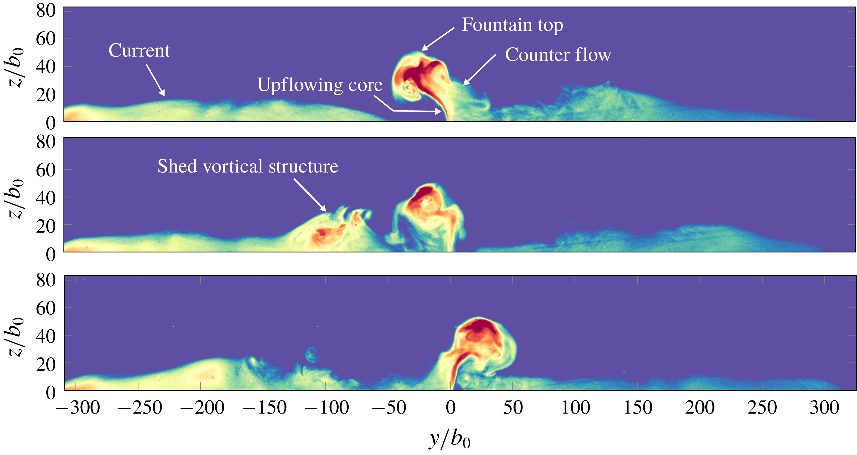
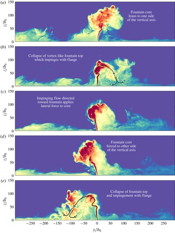
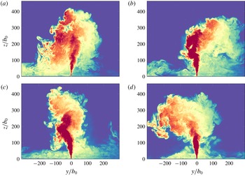
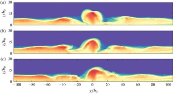
, i.e. the central section, are shown in figures 4–6 for the non-uniform, uniform and disorganised flapping behaviours, respectively. As we shall see, in each case, flapping entails that locally the fountain counterflow forms predominantly to one side of the slot at any given instant.
Viewed in a vertical section, it is evident that these fountains do not resemble the classic upflowing core and symmetric counterflow structure that is characteristic of round fountains. The structure is instead reminiscent of quasi-two-dimensional confined fountains (Debugne & Hunt Reference Debugne and Hunt2018) in that it consists of a slender upflowing core that undergoes a quasi-periodic swaying to each side of the slot. In the proximity of the fountain top, the core wraps up into vortex sheets that extend in the
 $x$
-direction (into the page, figures 4–6). Lateral excursions of the fountain are substantially greater than the spread in width of the upflowing core due to the coiling of these vortex sheets; lateral excursions appear to scale on the rise height as may be independently inferred from the top view on the flow (§ 2.2). These large-scale vortical structures are subsequently shed and collapse under gravity. It is the regular impingement of these structures with the horizontal flange, and subsequent interaction of the unsteady lateral current they create with the fountain core, that is instrumental to inducing the flapping behaviours.
The flapping mechanism is most clearly appreciated in figure 5 which has been annotated so as to link the lateral motion of the core with the shedding, left then right, of vortical structures from the fountain top. The flapping of the fountain to either side of the slot appears to be intrinsically linked to feedback between the fountain upflow and the (quasi-)regular shedding of large-scale vortical structures away from the fountain. The periodicity in the resulting flapping is less stark at larger rise heights (see figure 6 and movie 7) in which, for limited periods of time, the fountain is shrouded by a counterflow on both sides.
Non-uniform flapping. LIF visualisation of the central section for
 $\{L,b_{0}\}=\{300,0.5\}$
mm and
 $Fr_{0}=12.1$
(
 $Re_{0}\approx 41$
). Images spaced at time intervals of
 $\unicode[STIX]{x0394}t=2.3$
s (
 $\cong 1.0~w_{0}/g_{0}^{\prime }$
). Movie 5 available online.

Uniform flapping. LIF visualisation of the central section for
 $\{L,b_{0}\}=\{150,0.5\}$
mm and
 $Fr_{0}=24.1$
(
 $Re_{0}\approx 84$
). Images spaced at time intervals of
 $\unicode[STIX]{x0394}t=1.7$
s (
 $\cong 0.5~w_{0}/g_{0}^{\prime }$
). Movie 6 available online.

Disorganised flapping. LIF visualisation of the central section for
 $\{L,b_{0}\}=\{300,0.5\}$
mm and
 $Fr_{0}=57.6$
(
 $Re_{0}\approx 194$
). Images spaced at time intervals of
 $\unicode[STIX]{x0394}t=4.7$
s (
 $\cong 1.0~w_{0}/g_{0}^{\prime }$
). Movie 7 available online.

4 Analysis of experimental measurements
To the human eye, the local rise height variations and local lateral excursions reported in § 3 do not appear to be linked in an obvious manner. However, the following quantitative analysis of the flow patterns in terms of
 $Fr_{0}$
and
 $L/b_{0}$
, through developed diagnostics from which we are able to relate the motion in the vertical and in the lateral planes, confirms that, at the largest scale, these motions are underpinned by the same driving mechanism. First, the uniformity of the source is established (§ 4.1). Then the rise heights
 $z_{v}(x,t)$
, obtained from tracking the fountain top from the side view, are analysed (§ 4.2). Analysing the vertical fluctuations from this perspective in §§ 4.3 and 4.5, we show that diagnostics can be readily implemented to identify the flapping pattern from the side view alone. Top views of the flow are analysed in § 4.4 to quantify how lateral and vertical fluctuations are linked. Flapping patterns are categorised in § 4.6.
4.1 Uniformity
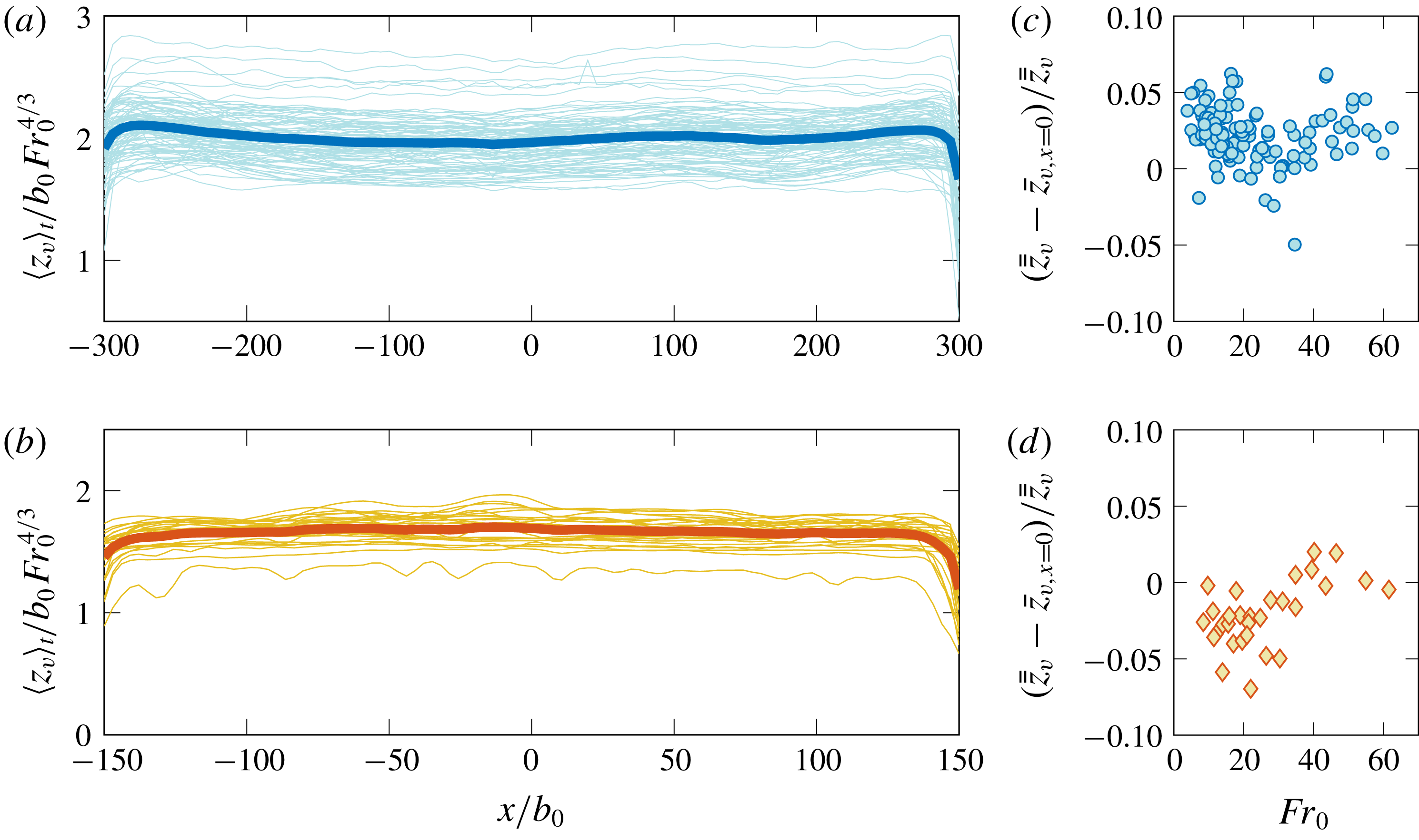
To assess the uniformity of the fountains along the length of the slot, in figure 7 the instantaneous time-averaged rise height
 $\left\langle z_{v}\right\rangle _{t}$
normalised by the source jet length
 $b_{0}Fr_{0}^{4/3}$
(Fischer et al.
Reference Fischer, List, Koh, Imberger and Brooks1979) is plotted against the spanwise coordinate
 $x/b_{0}$
. These profiles were obtained by averaging over a time interval
 $[0,T]$
the local rise height
 $z_{v}(x,t)$
at every
 $x$
-location, i.e.
 $$\begin{eqnarray}\left\langle z_{v}\right\rangle _{t}(x^{\prime })=\frac{1}{T}\mathop{\sum }_{t=0}^{T}z_{v}(x^{\prime },t),\quad x^{\prime }\in [-L/2,L/2].\end{eqnarray}$$
The duration
 $T$
was typically
 $O(10^{2})$
–
 $(10^{3})$
multiples of the buoyancy time scale
 $w_{0}/g_{0}^{\prime }$
, a time scale characteristic of the vertical fluctuations (§ 4.3), and the start time
 $t=0$
chosen to be well after the initial period of formation (§ 3.1). Shorter averaging times were unavoidable at high
 $Fr_{0}$
due to the increased rate at which the saline layer in the tank deepened. The profiles are convincingly uniform despite some irregularities at high
 $Fr_{0}$
. Judging from these profiles alone, the fountains might reasonably be regarded as two-dimensional. End effects are only evident as a marginal reduction in rise heights near the ends of the slot.
Normalised time-averaged rise height profiles. The profile for each individual fountain is plotted as a thin line and the average across all experiments is plotted as a thick line. (a) Set A (
 $L/b_{0}=600$
), plotting 97 experiments. (b) Set B (
 $L/b_{0}=300$
), plotting 28 experiments. For consistency with the fits (4.3), only profiles for
 $Fr_{0}\geqslant 10$
are included. (c,d) Normalised difference between the experiment-averaged and the centreline rise heights plotted against
 $Fr_{0}$
for sets A and B, respectively.

4.2 Rise height
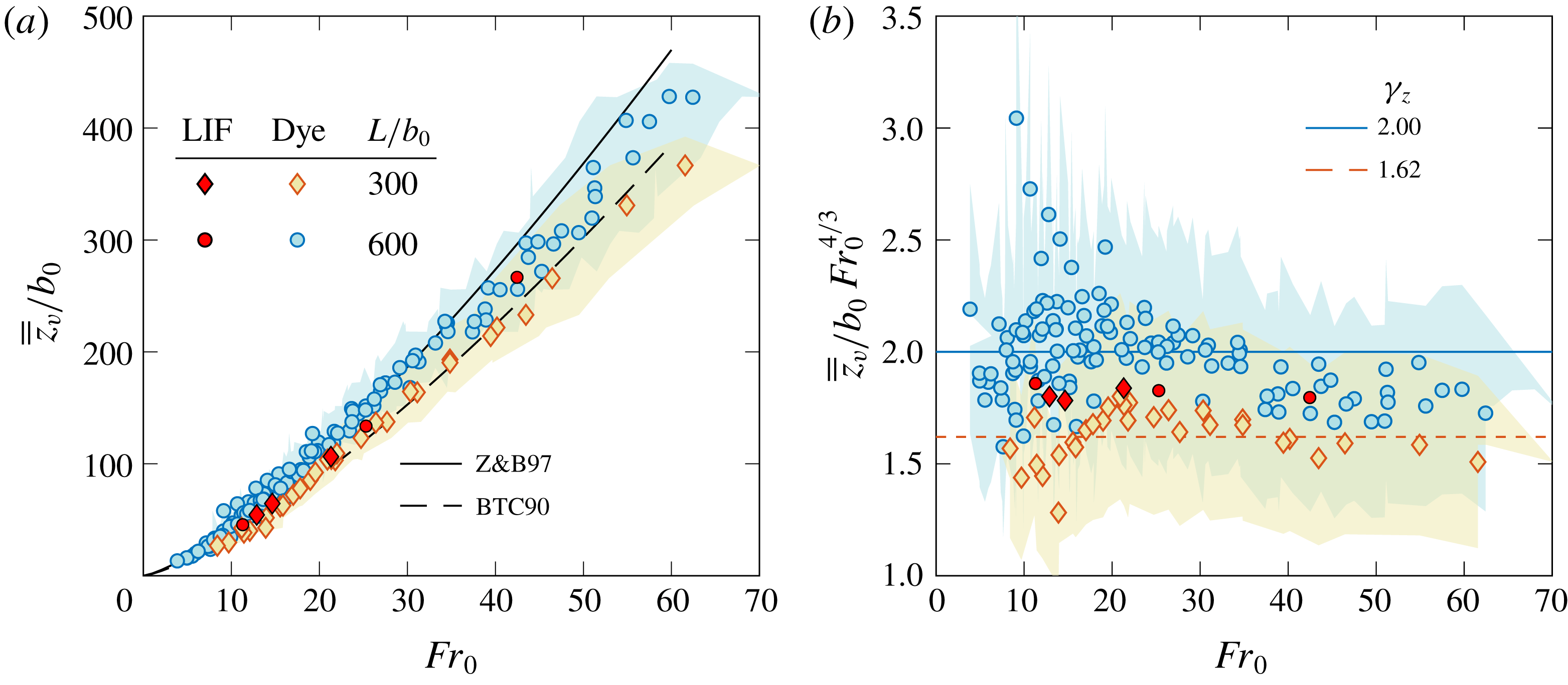
In figure 8, the double-averaged (spanwise and time) rise height
 $\overline{\overline{z}}_{v}$
scaled on
 $b_{0}$
is plotted against
 $Fr_{0}$
, where
 $$\begin{eqnarray}\overline{\overline{z}}_{v}=\frac{1}{T}\frac{1}{L}\mathop{\sum }_{t=0}^{T}\mathop{\sum }_{x=-L/2}^{L/2}z_{v}(x,t).\end{eqnarray}$$
Hereafter,
 $\overline{\overline{z}}_{v}$
is referred to as the experiment-averaged rise height. Also plotted are the (corrected) rise heights
 $\overline{z}_{v}$
from Baines et al. (Reference Baines, Turner and Campbell1990) and those from Zhang & Baddour (Reference Zhang and Baddour1997). Although rise heights are not the primary focus of our work, making the comparison between end-on,
 $\overline{z}_{v}$
, and spanwise,
 $\overline{\overline{z}}_{v}$
, rise heights is informative, and it is evident that our data for
 $\overline{\overline{z}}_{v}$
lie in close agreement with previous measurements of
 $\overline{z}_{v}$
. Lines of best fit to our data for
 $Fr_{0}\geqslant 10$
suggest that
 $$\begin{eqnarray}\overline{\overline{z}}_{v}/b_{0}=\unicode[STIX]{x1D6FE}_{z}\,Fr_{0}^{4/3},\end{eqnarray}$$
with
 $\unicode[STIX]{x1D6FE}_{z}=2.00$
for
 $L/b_{0}=600$
(blue circles) and
 $1.62$
for
 $L/b_{0}=300$
(orange diamonds). Both of our sets of rise height measurements fall predominantly between the fits of Baines et al. (Reference Baines, Turner and Campbell1990) and Zhang & Baddour (Reference Zhang and Baddour1997). The near absence of end effects (figure 7) explains, in part, why different boundary conditions at
 $x=\pm L/2$
, such as confining walls (Zhang & Baddour Reference Zhang and Baddour1997; Srinarayana et al.
Reference Srinarayana, Williamson, Armfield and Lin2010) or damping screens (Baines et al.
Reference Baines, Turner and Campbell1990), appear to have no adverse effect on the average rise heights. The difference in pre-factor of
 $19\,\%$
between our datasets is within experimental error (estimated as
 $7\,\%$
on
 $\overline{\overline{z}}_{v}/b_{0}$
and
 $14\,\%$
on
 $Fr_{0}$
, appendix B), and should not be interpreted as a dependence of rise height on
 $L/b_{0}$
. The influence of
 $L/b_{0}$
, both in terms of flapping behaviour and rise height, is discussed below.
At higher
 $Fr_{0}$
, the rise heights we measured fall marginally below the fits (4.3). This trend (for
 $Fr_{0}\gtrsim 30$
, figure 8
b) is expected to be a consequence of the free ends of the slot. Indeed, while we inspect the rise heights
 $z_{v}(x,t)$
above the slot only, i.e. for
 $x\in [-L/2,L/2]$
(4.2), as the fountain rises it spreads beyond
 $x=\pm L/2$
(e.g. figure 3
c). This spanwise expansion, absent from set-ups in which walls confine the ends, effectively represents a reduction in kinetic energy for the vertical motion above the slot. Therefore, fountains for which a spanwise spread is possible do not rise as high.
To make this argument more tangible, let us suppose that the fountain spreads at a rate
 $c_{y}$
in
 $y$
, and
 $c_{x}$
in
 $x$
at the ends. The total volume of fluid above the slot,
 $V_{in}$
, can be approximated as a trapezoid of length
 $L$
, so that
 $V_{in}=\left(4b_{0}+2c_{y}\overline{\overline{z}}_{v}\right)\,\overline{\overline{z}}_{v}L/2$
. Thus at high Froude numbers,
 $V_{in}\approx c_{y}\,\overline{\overline{z}}_{v}^{2}L$
. Similarly, the total volume of fluid lying beyond the ends,
 $V_{out}$
, can be approximated as two halves of an elliptic cone with axes
 $c_{x}\overline{\overline{z}}_{v}$
and
 $c_{y}\overline{\overline{z}}_{v}$
, so that
 $V_{out}\approx \unicode[STIX]{x03C0}c_{x}c_{y}\overline{\overline{z}}_{v}^{3}/3$
. Alternative geometric shapes can be proposed for
 $V_{in}$
and
 $V_{out}$
, yet it seems inevitable that
 $V_{in}\propto \overline{\overline{z}}_{v}^{2}L$
and
 $V_{out}\propto \overline{\overline{z}}_{v}^{3}$
. It follows that
 $$\begin{eqnarray}\frac{V_{out}}{V_{in}}\sim c_{x}\frac{\overline{\overline{z}}_{v}}{L}.\end{eqnarray}$$
Thus, the greater the ratio of
 $\overline{\overline{z}}_{v}$
to
 $L$
, the greater the volume and, by extension, kinetic energy that is imparted to the spanwise motion for
 $|x|>L/2$
. Since greater rise heights are achieved on increasing
 $Fr_{0}$
, the ratio (4.4) is consistent with the view that the rise heights will depart from (4.3) at higher
 $Fr_{0}$
. Moreover, the onset of that departure is expected to be a function of the ratio
 $\overline{\overline{z}}_{v}/L$
. The relative difference between the centreline (taken to be the central 1 % span,
 $x\in [-0.005L,0.005L]$
) and the experiment-averaged rise height is shown in figure 7(c,d). Evidently, the centreline of the fountain rises marginally higher in most cases than the span average for
 $L/b_{0}=600$
(figure 7
c) and is marginally lower for
 $L/b_{0}=300$
(figure 7
d). Differences in rise height are within 10 % of the span-averaged rise height and are smaller than the scale of typical vertical fluctuations (see § 4.3).
For the vast majority of our experiments, the rise heights follow (4.3); even at high
 $Fr_{0}$
, the observed departure from (4.3) is relatively small. Therefore, we proceed on the premise that our measurements of line fountain rise height lie in good agreement with previous measurements with the mean across our datasets being
 $\overline{\overline{z}}_{v}/b_{0}=1.81Fr_{0}^{4/3}$
.
(a) Experiment-averaged rise height
 $\overline{\overline{z}}_{v}/b_{0}$
against
 $Fr_{0}$
from our side view
 $(x{-}z)$
measurements. Also plotted are the fits by Zhang & Baddour (Reference Zhang and Baddour1997) and Baines et al. (Reference Baines, Turner and Campbell1990) (1.1) from their end view
 $(y{-}z)$
measurements. Shaded regions bound our experimental error. The dark red shaded symbols indicate data extracted from our LIF visualisations. (b) Experiment-averaged rise height data from (a) shown on a compensated plot. The trends shown in the data indicate a departure from a 4/3 power-law scaling at higher
 $Fr_{0}$
.

4.3 Vertical fluctuations
Fountains are typified by quasi-periodic fluctuations whose scaling, both in amplitude and frequency, is often revelatory of the underlying dynamics that govern their behaviour (Williamson et al. Reference Williamson, Srinarayana, Armfield, McBain and Lin2008; Srinarayana et al. Reference Srinarayana, Williamson, Armfield and Lin2010; Burridge & Hunt Reference Burridge and Hunt2013). For the fountains studied herein, there are two principal fluctuating components: one vertical, of smaller amplitude and shorter period, and one lateral, of larger amplitude and longer period. Viewed from the side, vertical fluctuations appear as a local phenomenon in that there is no obvious coherence between fluctuating motions along the span (cf. movies 2–4 supporting figure 3 a–c). By contrast, lateral fluctuations (as viewed from the top) appear as a global phenomenon in that they form organised patterns, for example, with the fountain swaying back and forth as a whole.
The amplitude of vertical fluctuations,
 $\unicode[STIX]{x1D6FF}z_{v}$
, calculated as twice the average of the standard deviations of the experiment-averaged rise heights
 $\overline{\overline{z}}_{v}$
, is plotted against
 $Fr_{0}$
in figure 9. Two standard deviations provided a good measure for the peak-to-trough amplitude of typical fluctuations (based on visual inspection), which motivated our choice of definition for
 $\unicode[STIX]{x1D6FF}z_{v}$
. Moreover, deviations about the mean rise height profile
 $\left\langle z_{v}\right\rangle _{t}(x)$
were uniform along
 $x$
in the time average and distributed normally, so that the single measure
 $\unicode[STIX]{x1D6FF}z_{v}$
is representative of the whole fountain.
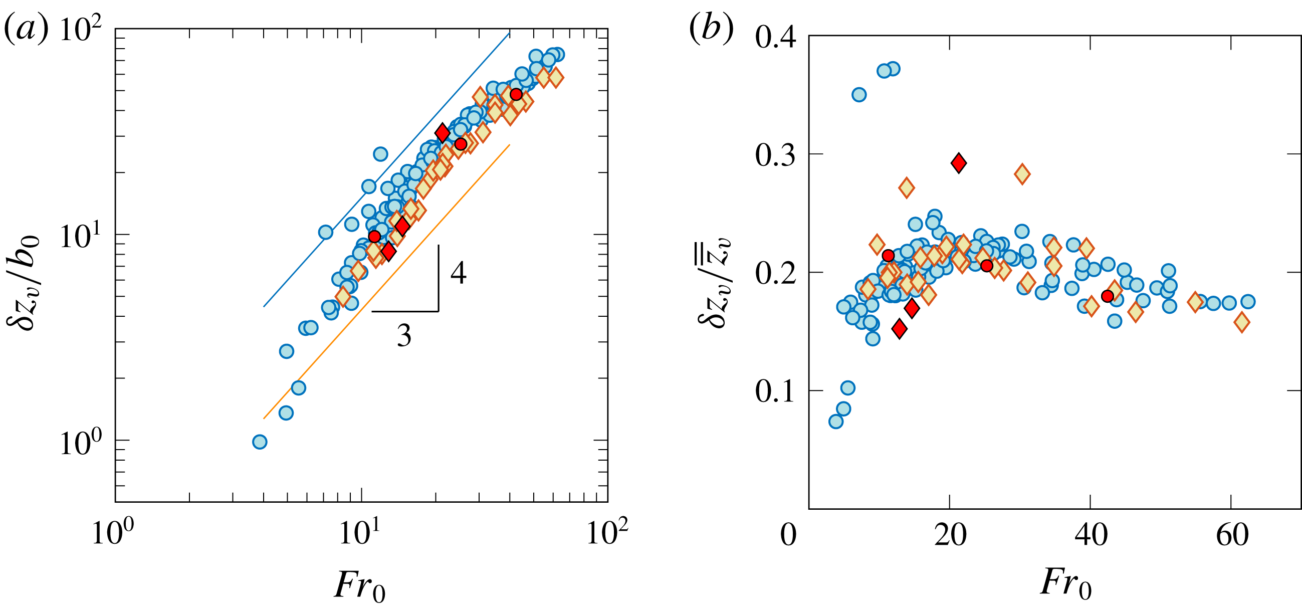
The fluctuations echo our observations made about the rise heights (figure 8). First,
 $\unicode[STIX]{x1D6FF}z_{v}$
scales on
 $Fr_{0}^{4/3}$
, with the fluctuations being slightly lower for set B. This scaling is also evident from figure 9(b) where, for
 $Fr_{0}\lesssim 30$
, the fluctuations represent a near constant fraction of the experiment-averaged rise height; at circa 20 %, discounting a few outliers, this fraction is somewhat higher than for round fountains (
 ${\sim}15\,\%$
, Burridge & Hunt Reference Burridge and Hunt2013). Second,
 $\unicode[STIX]{x1D6FF}z_{v}$
departs from the
 $4/3$
-scaling at higher values of
 $Fr_{0}$
. This departure is likely to be due to the reasons laid out in § 4.2, the fountain expanding beyond the ends of the source so that a fraction of kinetic energy is unavailable to drive the vertical motion over
 $x\in [-L/2,L/2]$
.
Amplitude of vertical fluctuations
 $\unicode[STIX]{x1D6FF}z_{v}$
against
 $Fr_{0}$
, normalised (a) by the slot half-width
 $b_{0}$
and (b) by the experiment-averaged rise height. Symbols as in figure 8.

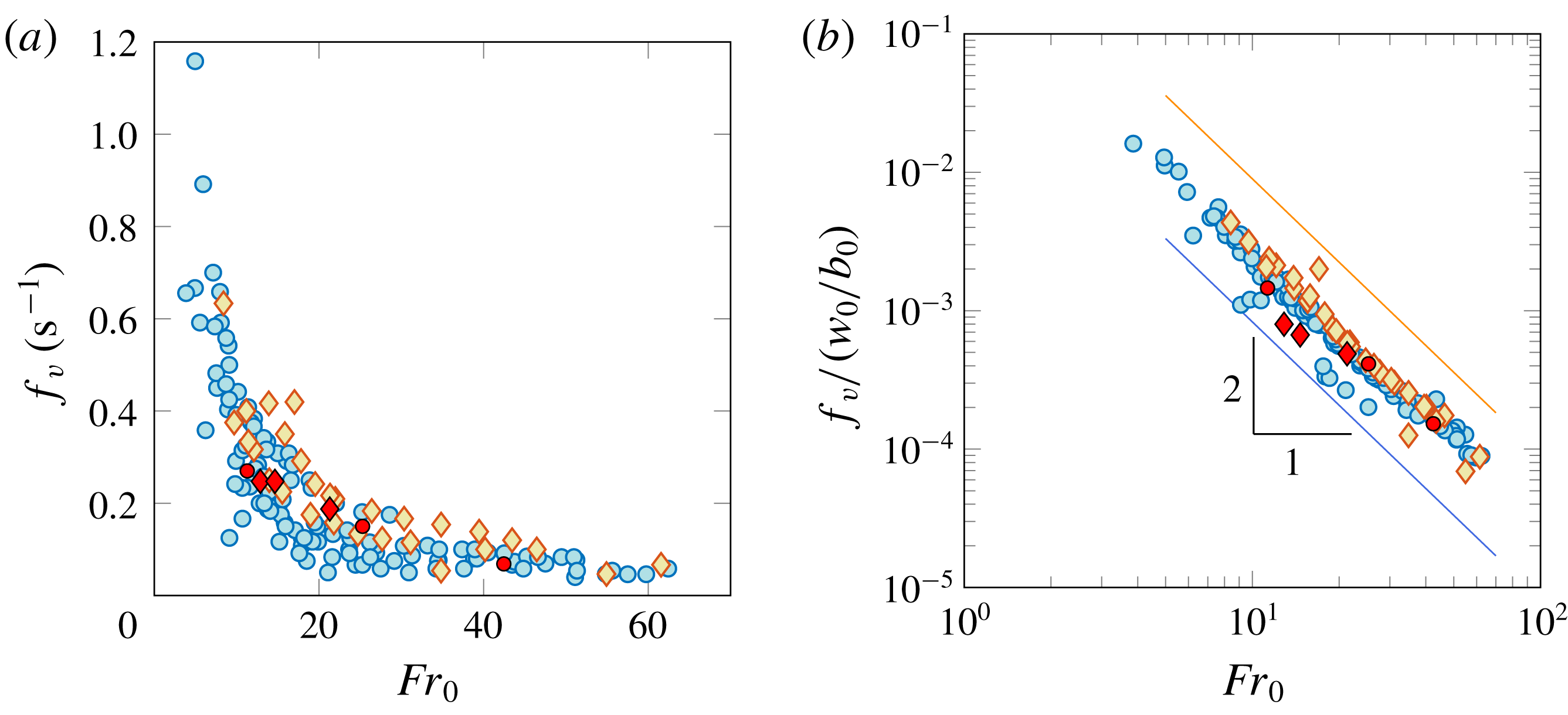
Characteristic frequency of vertical fluctuations
 $f_{v}$
against
 $Fr_{0}$
, (a) dimensional frequency and (b) frequency normalised by the inverse of the time scale
 $b_{0}/w_{0}$
. Vertical error bars are smaller than the symbol size. In (b), lines of best fit (4.5) have a slope of
 $-2$
and are offset for ease of reading. Symbols as in figure 8.

Next, we inspect the typical (or dominant) frequencies for the vertical motion,
 $f_{v}$
. By applying a fast Fourier transform to the signal
 $z_{v}(x=x^{\prime },t)$
, the dominant frequency was extracted at each location
 $x=x^{\prime }$
. The distribution of the resulting frequencies (one for each
 $x^{\prime }$
) was typically bimodal, with the larger mode corresponding to the first dominant frequency, and a distinctly lower mode corresponding to the second. Therefore, to obtain a characteristic frequency
 $f_{v}$
representative of the whole fountain, we define
 $f_{v}$
as the mode of the individual frequencies sampled at each
 $x$
-location.
The frequency
 $f_{v}$
(
 $\text{s}^{-1}$
) of the vertical fluctuations is plotted against
 $Fr_{0}$
in figure 10(a) and normalised by the inverse of the time scale
 $b_{0}/w_{0}$
in figure 10(b). Evidently, vertical frequencies decrease with increasing
 $Fr_{0}$
, consistent with the view that the amplitudes of characteristic fluctuations increase with
 $Fr_{0}$
(figure 9). The frequencies in both measurement sets are close in magnitude and follow the same trend. Imposing an exponent of
 $-2$
as the nearest integer power, lines of best fit follow
 $$\begin{eqnarray}f_{v}/(w_{0}/b_{0})=\unicode[STIX]{x1D6FE}_{v}\,Fr_{0}^{-2},\end{eqnarray}$$
with
 $\unicode[STIX]{x1D6FE}_{v}=0.249$
for
 $L/b_{0}=600$
(blue circles) and
 $0.299$
for
 $L/b_{0}=300$
(orange diamonds). Coefficients of determination for the fits (4.5) are
 $R^{2}=0.95$
and
 $0.96$
for sets A and B, respectively. We reason in appendix B that the differences in pre-factor in (4.5) are within experimental error. Figure 10 and expressions (4.5) therefore indicate that the vertical frequencies scale on
 $w_{0}Fr_{0}^{-2}/b_{0}=g_{0}^{\prime }/w_{0}$
, the inverse of the buoyancy time scale. This scaling is characteristic of fountains that are sufficiently highly forced.
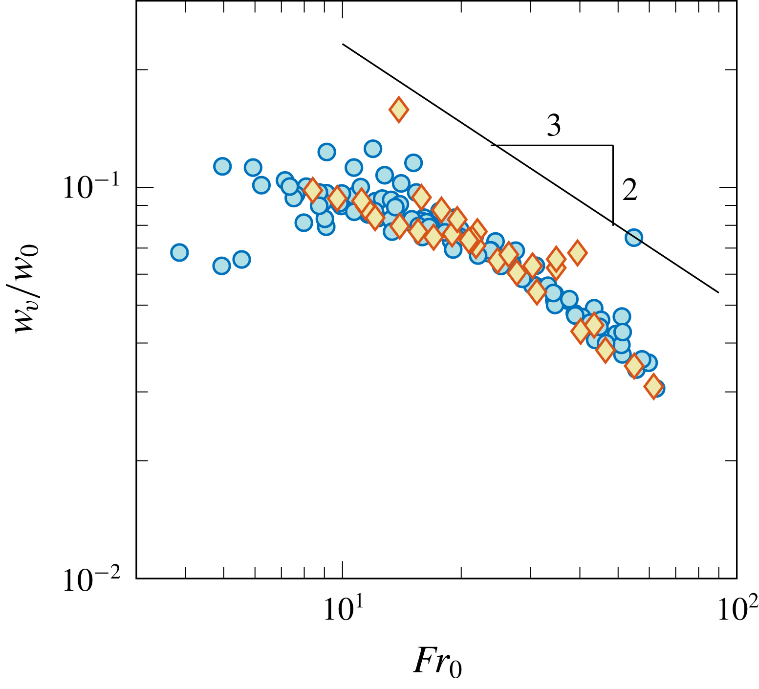
The same scaling was identified by Burridge & Hunt (Reference Burridge and Hunt2013) for the frequencies of a fluctuating, forced and round fountain top. Their scaling was developed by considering the relevant length and velocity scales for vertical fluctuations from a theoretical standpoint, and the relevant time scale deduced by combining them appropriately. Proceeding in reverse, we may infer a scale for the characteristic velocities
 $w_{v}$
of vertical fluctuations. Since
 $\unicode[STIX]{x1D6FF}z_{v}/b_{0}\propto Fr_{0}^{4/3}$
(figure 9) and
 $f_{v}/(w_{0}/b_{0})\propto Fr_{0}^{-2}$
(figure 10), we infer
 $w_{v}/w_{0}\propto Fr_{0}^{-2/3}$
, which corresponds to the theoretical scaling for two-dimensional fountains (van den Bremer & Hunt Reference van den Bremer and Hunt2014b
). Although
 $w_{v}$
was not measured directly in our experiments, an estimate of
 $w_{v}$
can be gained from the time rate of change of
 $z_{v}$
. In appendix G we define
 $w_{v}$
as the root-mean-square of
 $\text{d}z_{v}/\text{d}t$
and confirm that
 $w_{v}$
scales on
 $w_{0}Fr_{0}^{-2/3}$
, in accord with two-dimensional theory.
4.4 Lateral fluctuations
As raised in § 2.2, the irregular and weak contrasts between the fountain and the background precluded us from reliably tracking the lateral excursions from top views. Whilst measuring the amplitude of lateral fluctuations requires a well-defined outline, measuring the frequency of these fluctuations does not. If one could count the number of times
 $n$
a fountain flaps over the duration
 $T$
of an experiment, then an estimate for the flapping frequency would be given by
 $n/T$
. In Debugne & Hunt (Reference Debugne and Hunt2018), we implemented an ‘eddy-counting’ approach which rested on a similar principle, and through which the formation frequency of large eddies in meandering fountains was identified. We adapted this approach, not to count eddies, but to count flapping events.
Proceeding as described in appendix E,
 $(y,t)$
-time series were constructed for each experiment, the dominant frequencies extracted at each
 $y$
-location through Fourier transforms and their mode calculated to determine
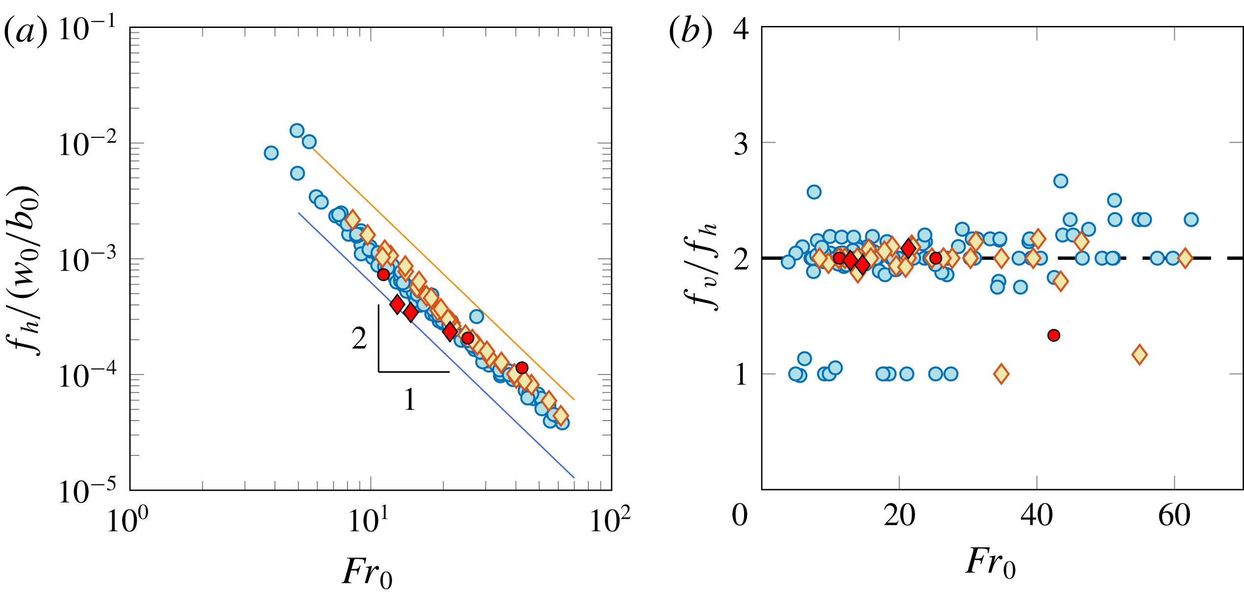
 $f_{h}$
, the dominant frequency of the lateral fluctuations. The resulting frequencies are plotted against
 $Fr_{0}$
in figure 11(a). Akin to the vertical frequencies (figure 10), the lateral frequencies closely follow an inverse square power law. Imposing an exponent of
 $-2$
, lines of best fit are
 $$\begin{eqnarray}f_{h}/(w_{0}/b_{0})=\unicode[STIX]{x1D6FE}_{h}\,Fr_{0}^{-2},\end{eqnarray}$$
with
 $\unicode[STIX]{x1D6FE}_{h}=0.125$
for
 $L/b_{0}=600$
(blue circles) and
 $0.148$
for
 $L/b_{0}=300$
(orange diamonds), with
 $R^{2}=0.98$
for both fits. The pre-factors
 $\unicode[STIX]{x1D6FE}_{h}$
in (4.6) are almost exactly half the pre-factors
 $\unicode[STIX]{x1D6FE}_{v}$
in (4.5) for both sets. Plotting the ratio of
 $f_{v}$
to
 $f_{h}$
(figure 11
b) confirms this observation: the ratio
 $f_{v}/f_{h}$
scatters around a value of two, with a few outliers falling mostly on harmonics.
Figure 11(b) reveals a key dynamic feature of line fountains, namely, that the largest (dominant) vertical fluctuations are caused by lateral swaying, i.e. by the flapping motions. Based on this premise, a ratio of
 $f_{v}/f_{h}=2$
indeed makes sense, since for every lateral sway to one side of the source, the fountain passes above the source (i.e. through the central plane) twice. This finding explains why the vertical fluctuations (figure 13) arrange into patterns reminiscent of the lateral motion: at the largest scale, the lateral motion dictates the vertical fluctuations. Note that the relationship
 $f_{v}/f_{h}=2$
remains valid at large values of
 $Fr_{0}$
, despite the rather disorganised appearance (to the naked eye) of images such as figure 3(c).


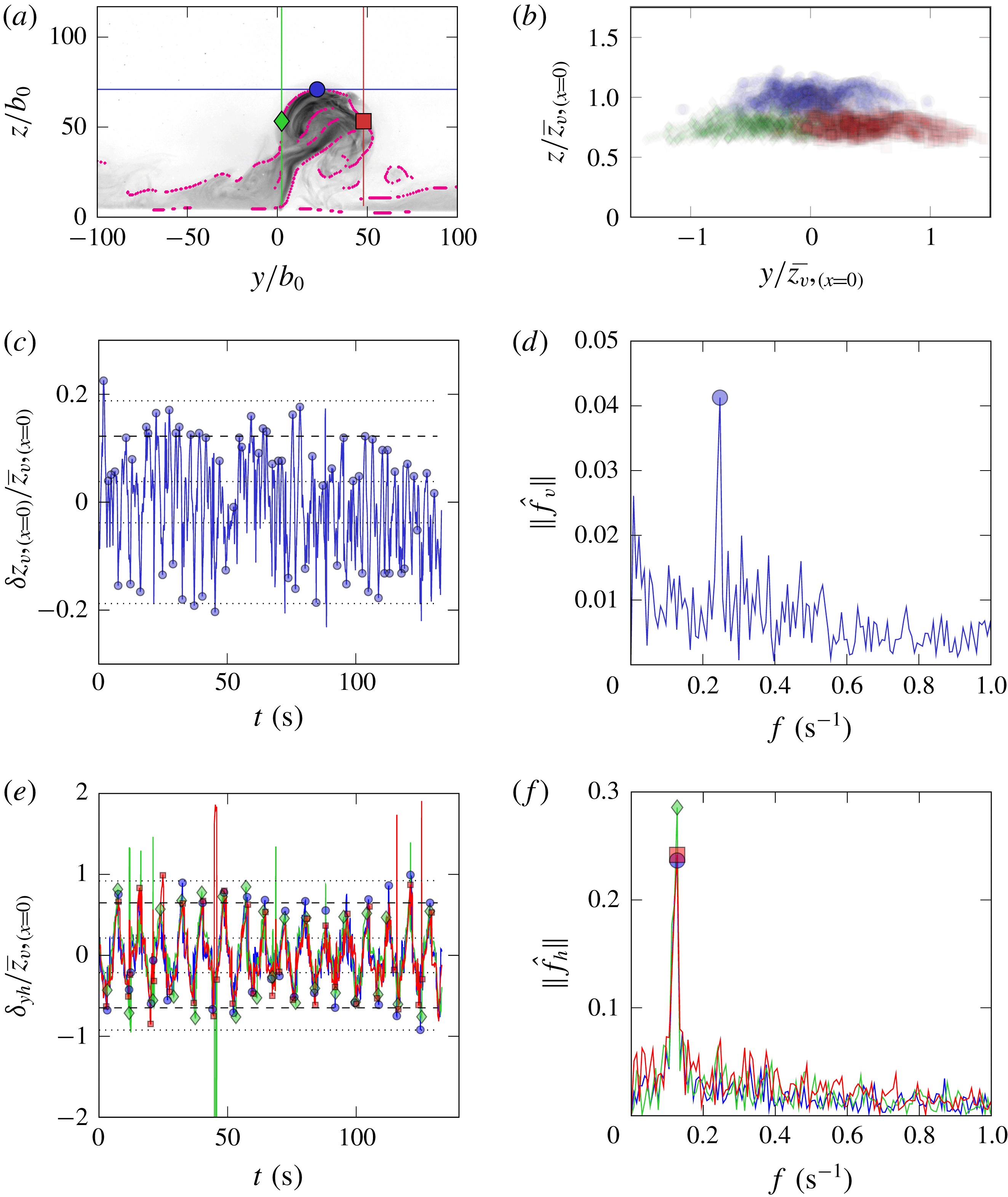
From the LIF visualisations, the lateral excursions were quantified and a complementary suite of frequency measurements for the lateral and vertical fluctuations acquired. The technique we implemented to extract these quantities is illustrated in appendix F for an example experiment. Regarding the vertical motion, mean rise heights
 $\overline{z}_{v,(x=0)}$
and rise height fluctuations
 $\unicode[STIX]{x1D6FF}z_{v,(x=0)}$
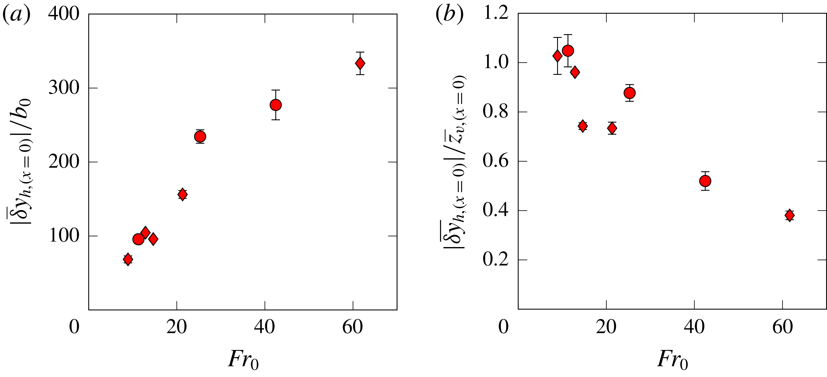
measured in the illuminated central section are superimposed onto figures 8 and 9, and again indicate good agreement between the LIF and dye-attenuation approaches. Regarding lateral excursions, a minimum representative value might reasonably be anticipated to be comparable with the scale of the vertical fluctuations (i.e. circa 20 % of the rise height, figure 9) on account of these fluctuations being on the scale of a notional eddy. Flapping enhances this lateral excursion as the upflowing core then leans to either side of the slot (e.g. figure 4); based on our observations, a maximum representative value for a lateral excursion is expected to be comparable with the rise height. The actual magnitude of the time-averaged peak lateral excursions acquired from the LIF data, relative to the slot width and rise height, is plotted in figure 12(a,b) against
 $Fr_{0}$
. Consistent with our observations, whilst lateral excursions increase in scale as the fountain rises higher (increasing
 $Fr_{0}$
, figure 12
a), as a fraction of the mean rise height measured in the illuminated plane, these excursions decrease (figure 12
b). At lower
 $Fr_{0}$
, for which flapping occurs at a well-defined frequency, the lateral excursions are comparable to the rise height. At higher
 $Fr_{0}$
, the disorganised flapping results in the magnitude of the lateral excursions decreasing and approaching what would be expected if the fountain was symmetric (Hunt & Burridge Reference Hunt and Burridge2015).
As an aside, we attempted to inspect frequencies associated with secondary peaks in the Fourier transforms of the vertical motion. Since the frequencies of the most energetic fluctuations are those associated with the global lateral motion, we questioned whether secondary peaks were indicative of smaller, locally driven fluctuations. In a number of time records for the instantaneous rise height (e.g. figure 20 c), peaks could be identified in super-harmonics of the base frequency. These peaks are most likely to result from the nonlinear interaction of the fluctuations with the base frequency. Identifying these super-harmonics consistently for each experiment, however, proved to be inconclusive owing to the turbulent nature of the fountain top.
Magnitude of mean lateral excursions versus
 $Fr_{0}$
as obtained from the LIF experiments: (a) scaled on the source half-width and (b) scaled on the time-averaged rise height measured on the illuminated central section.

4.5 Spatio-temporal contour maps for the vertical fluctuations
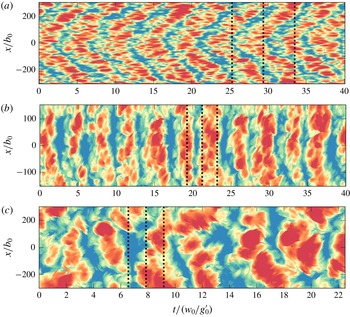
Signatures for the lateral behaviours of turbulent forced line fountains. Contour maps of the vertical fluctuations,
 $z_{v}(x,t)-\left\langle z_{v}\right\rangle _{t}(x)$
. (a) Diagonal banding (chevrons) characteristic of non-uniform flapping (
 $L/b_{0}=600$
,
 $Fr_{0}=10.2$
); (b) vertical banding of uniform flapping (
 $L/b_{0}=300$
,
 $Fr_{0}=26.4$
); and (c) broken banding of disorganised flapping (
 $L/b_{0}=600$
,
 $Fr_{0}=51.3$
). Dotted lines demark the time instants which correspond to the images in figure 3(a–c). In each contour map, the colour scale ranges between minus and plus the largest vertical fluctuation (in absolute value).

Figures 9 and 10 each plot a single amplitude and a single frequency per experiment, respectively. As such, the two figures separate the spatial and temporal aspects of the vertical fluctuations. An alternative format for visualising the vertical fluctuations in space and time simultaneously is presented in figure 13. Each of the three contour maps therein plots, at location
 $x^{\prime }$
and instant
 $t^{\prime }$
, the difference between the instantaneous rise height
 $z_{v}(x=x^{\prime },t=t^{\prime })$
and the time-averaged rise height at that location,
 $\left\langle z_{v}\right\rangle _{t}(x=x^{\prime })$
. Thus, these maps give an
 $(x,t)$
, local and instantaneous, representation of the vertical fluctuations. To enable direct comparison between the vertical fluctuations and observations made in § 3, the contours in figure 13(a–c) are calculated for the experiments shown in figure 3(a–c) that typify the three distinct lateral behaviours.
Plotted thus, it becomes evident that the vertical fluctuations that occur along the span of the fountain are correlated. The fluctuations are arranged into regular patterns of bands with alternating positive and negative fluctuations. The width of each band (i.e. in time) corresponds to a fluctuating period (cf. the frequencies in figure 10), whilst its elevation corresponds to a fluctuating amplitude. The pervasiveness of these patterns indicates that, at the largest scale, the vertical fluctuations are not a local process, but instead are governed by a regular, global process. This assertion becomes clearer on recognising that the patterns in figure 13(a–c), respectively, are signatures for the non-uniform, uniform and disorganised flapping lateral behaviours noted earlier in our observations of the flow in the top views:
(i) Figure 13(a): the chevrons imply that, at any given time, the rise height fluctuations alternate sign along the span
 $x$
in an organised manner. For example, when fluctuations are positive in the central region, they are negative in neighbouring regions. The presence of chevrons, or indeed of any regular diagonal pattern, therefore indicates that the rise height fluctuations along the span are alternately in and out of phase. This is the same observation as we made for the lateral fluctuations in figure 3(a), where the top views clearly show the fountain oscillating about the slot.
(ii) Figure 13(b): the vertical banding indicates that the fluctuations are uniform along the span. Correspondingly, in the top views of figure 3(b), the fountain flaps uniformly.
(iii) Figure 13(c): the regular banded structure is lost and the contours depict less organised, broken bands. This signature is consistent with figure 3(c), where large-scale structures at the fountain top appear to dominate the flow.

We conclude that the vertical fluctuations bear the imprint of the lateral swaying of the fountain, i.e. the motions in the vertical and lateral planes are connected. Finally, we note that each band is comprised of a number of distinct structures whose spanwise extent is constant (approximately) in a given regime, but clearly increases across the regimes in figure 13(a–c) – a trend consistent with the observations made regarding the scale of eddying structures in § 3.2.
4.6 Parameter space for flapping patterns
In § 3, we established that different lateral behaviours occur at different
 $Fr_{0}$
-thresholds depending on the value of
 $L/b_{0}$
. Intuitively, we would expect the fountain to behave more uniformly along the span if the characteristic length scale of structures at the top were comparable with, rather than small compared with, the span. In the hypothetical limiting case of the fountain consisting of a single coherent structure, for instance, the flow sways back and forth as one.
Although we do not have a direct measure for the size of individual structures from our visualisations, it is reasonable to assume that they scale on the length relevant to forced line fountains, i.e. on
 $b_{0}Fr_{0}^{4/3}$
and, by extension, on
 $\overline{\overline{z}}_{v}$
(§ 4.3). The ratio of the size of structures to the length of the fountain should therefore be proportional to
 $\overline{\overline{z}}_{v}/L$
. This suggests thresholds for the different flapping behaviours in terms of the height-to-length ratio
 $\overline{\overline{z}}_{v}/L$
.
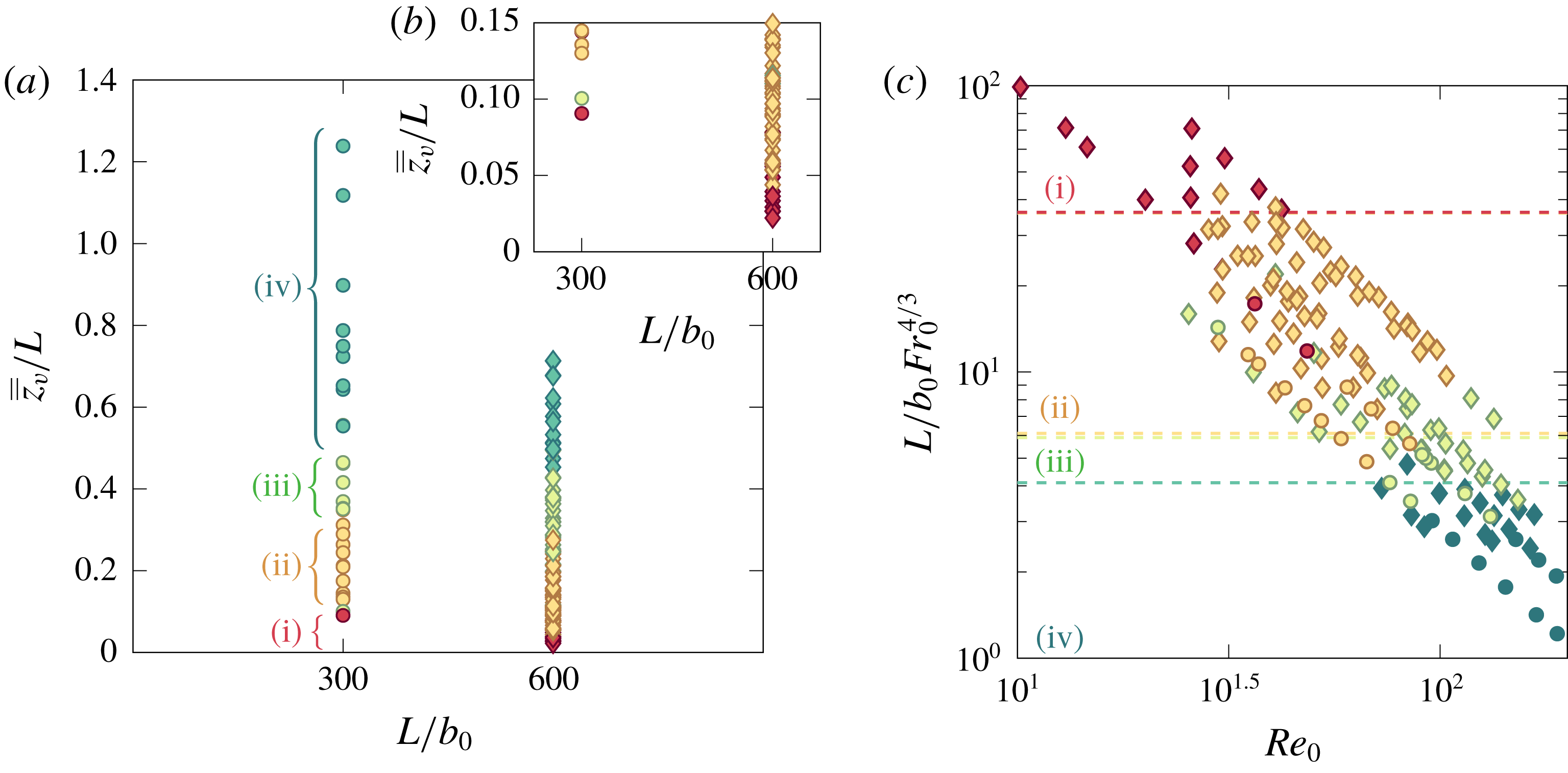
To determine the flapping behaviour, we constructed contour maps of the vertical fluctuations, such as those shown in figure 13, for each experiment and classified the flow into the following categories according to the signature that emerged: (i) non-uniform flapping with more than one and a half winds, i.e. wavelengths less than
 $2L/3$
, as is characteristic of laminar fountains, (appendix D), and for turbulent fountains, either (ii) non-uniform flapping with diagonal bands or chevrons (figure 13
a), (iii) uniform flapping with vertical bands (figure 13
b) or (iv) uniform flapping with broken bands (figure 13
c). The resulting regime diagram, plotting
 $\overline{\overline{z}}_{v}/L$
against
 $L/b_{0}$
, is shown in figure 14 where each experiment has been colour coded according to its flapping behaviour. Although we observe some variability, the flapping behaviours can be delineated by constant values of the height-to-length ratio
 $\overline{\overline{z}}_{v}/L$
as follows:
(i)
$\overline{\overline{z}}_{v}/L\lesssim 0.05$
or
$L/b_{0}Fr_{0}^{4/3}\gtrsim 36$
, non-uniform flapping,
$L_{w}\lesssim 2L/3$
;(ii)
$0.05\lesssim \overline{\overline{z}}_{v}/L\lesssim 0.30$
or
$6\lesssim L/b_{0}Fr_{0}^{4/3}\lesssim 36$
, non-uniform flapping,
$L_{w}\approx 2L/3$
;(iii)
$0.30\lesssim \overline{\overline{z}}_{v}/L\lesssim 0.45$
or
$4\lesssim L/b_{0}Fr_{0}^{4/3}\lesssim 6$
, uniform flapping; and(iv)
$\overline{\overline{z}}_{v}/L\gtrsim 0.45$
or
$L/b_{0}Fr_{0}^{4/3}\lesssim 4$
, disorganised flapping,








 $L_{w}$
being the longitudinal wavelength of the flapping.
(a) Regime diagram for classification of lateral flapping behaviour in terms of
 $\overline{\overline{z}}_{v}/L$
and
 $L/b_{0}$
, colour coded for the characteristic signatures in the contour maps of vertical fluctuations (figure 13). Colour code as follows: (i) red, non-uniform with wavelengths less than
 $2L/3$
(appendix D); (ii) orange, diagonal bands, including chevrons (figure 13
a); (iii) green, vertical bands (figure 13
b); and (iv) turquoise, disorganised broken vertical bands (figure 13
c). (b) The inset provides a zoomed view onto
 $\overline{\overline{z}}_{v}/L\leqslant 0.15$
. (c) An alternative regime diagram in which the ratio of the slot length to the normalised predicted rise height is plotted against
 $Re_{0}$
.

Interestingly, this delineation entails that
 $\overline{\overline{z}}_{v}/L$
governs which flapping pattern is adopted and how two-dimensional a flow should be regarded. Regarding the latter, we recall from § 4.2 that rise heights begin to depart from the two-dimensional theoretical scaling for larger
 $Fr_{0}$
, and by extension for larger
 $\overline{\overline{z}}_{v}/L$
. Thus, despite their instantaneous uniformity along the span, uniformly flapping line fountains, which form only for the larger values of
 $\overline{\overline{z}}_{v}/L$
considered, cannot be regarded as the more two-dimensional of the fountains examined (though in a time-averaged sense, cross-sections through uniformly flapping and non-uniformly flapping line fountains would be identical).
Proceeding on the basis that the spanwise and vertical length scales of the largest-scale structures are comparable, so that specifically the spanwise extent of structures scales as
 $x_{e}\sim b_{0}Fr_{0}^{4/3}$
, then the number
 $m$
of structures along the span of a fountain top of length
 $L_{t}$
would be anticipated to scale as
 $m\sim L_{t}/b_{0}Fr_{0}^{4/3}$
. If we now postulate that the basic arrangement that is required to form a lateral flapping pattern with wavenumber
 $k$
comprises of structures vertically above the source and structures deflected to either side, then a minimum of
 $m=m_{min}=7$
is required to achieve
 $k=3/2$
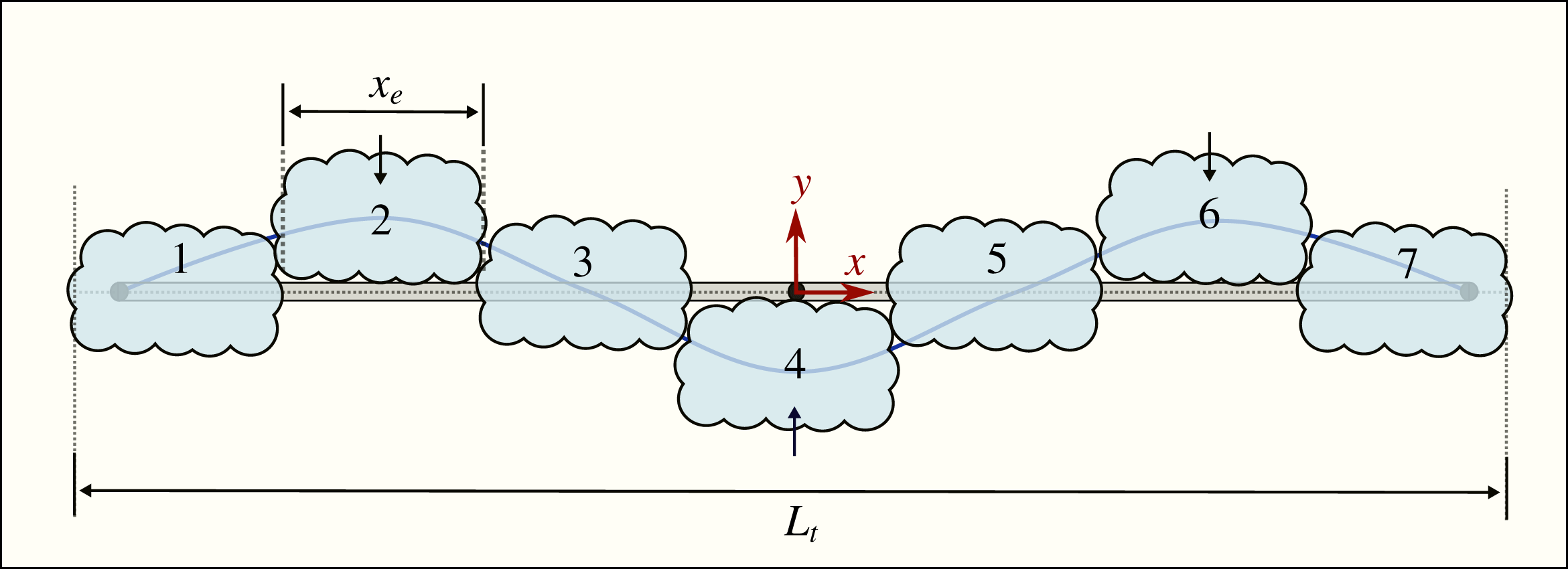
. Such an arrangement is shown schematically in figure 15 with the largest-scale structures numbered. Introducing
 $c_{e}$
as a constant of proportionality, so that
 $x_{e}=c_{e}~b_{0}Fr_{0}^{4/3}$
, and noting that the minimum number of structures
 $m=m_{min}(k)$
corresponds to the maximum (or threshold) source Froude number
 $Fr_{0}=Fr_{0,max}$
for the given behaviour, then we have
 $$\begin{eqnarray}Fr_{0,max}=\left(\frac{L_{t}}{b_{0}}\right)^{3/4}\left(\frac{1}{c_{e}~m_{min}}\right)^{3/4}.\end{eqnarray}$$
The length
 $L_{t}$
of a fountain whose ends are free increases with
 $Fr_{0}$
. However, for the modest increases relative to
 $L$
observed in the non-uniform flapping regime, it is not unreasonable to approximate the length of the fountain top by the length of the slot. Substituting
 $L_{t}/b_{0}=L/b_{0}$
and
 $m_{min}=7$
in (4.7), we predict
 $Fr_{0,max}=\{16.8,28.2\}$
for
 $L/b_{0}=\{300,600\}$
with
 $c_{e}=1$
. In our experiments, the corresponding threshold values of the source Froude number at which non-uniform flapping was maintained (§ 3.2) were
 $Fr_{0,max}=\{20,27\}$
for
 $L/b_{0}=\{300,600\}$
. Given the approximations made and the simple form proposed for the basic arrangement of structures (figure 15), these predictions show remarkably good agreement with the experimental values.
Plan view of a fountain top, of length
 $L_{t}$
, depicting the minimum number (
 $m_{min}=7$
) of large-scale structures each with spanwise length
 $x_{e}$
that arrange to form a pattern with wavenumber
 $k=3/2$
, as is characteristic of non-uniform flapping. Structures numbered
 $\{1,3,5,7\}$
are in the vertical plane of the source and structures
 $\{2,4,6\}$
are deflected to either side.

5 Concluding remarks
We have established the fundamental structure of free turbulent line fountains by means of an experimental study in which aqueous-saline fountains were formed on ejecting dense saline solution vertically upwards into a freshwater environment from a source in a horizontal plane. Potential applications of these flows include the environmental control of a room (wherein occupant comfort may be achieved by the injection of cool air upwards as part of an underfloor air distribution system, or by the injection of warm air downwards from a device at ceiling level) and the fate of dense pollutants released into the ocean from a cracked pipeline. As an approximation to the theoretical idealisation of a line, slender rectangular sources whose length
 $L$
exceeds the half-width
 $b_{0}$
by two orders of magnitude, specifically
 $L/b_{0}=\{600,300\}$
, were designed and tested to ensure uniform release conditions were achieved. A summary of our experimental measurements is presented in table 3. Two essential features distinguish these from previous experiments: our fountains were produced at considerably higher aspect ratios
 $L/b_{0}$
and, not confined by end walls, were free to develop in all three dimensions. Both features were instrumental in shaping fountain behaviour.
Motivation for this study was threefold. First, in contrast to fountains from circular sources, progress in the theoretical modelling of line fountains has been stifled by an absence of observational data to such an extent that models currently exist only for the initial rise, i.e. prior to the establishment of a counterflow. Even a grasp of the basic structure of the flow along the span, as would be observed on viewing the fountain from above and from the side, was absent. Second, theoretical models for fountains from circular sources rely on a delineation of the upflowing core from the counterflow and so we wished to examine the internal structure of line fountains in order to understand how the core and counterflow interact. Third, we wished to establish whether a line fountain could reasonably be regarded as two-dimensional: given the high aspect ratio of the sources considered, broadly uniform conditions might have been anticipated along the span (other than at the free ends) for release conditions that yield rise heights that are small relative to the slot length. This was not the case.
Synchronously viewing the fountain externally from the side and above, and internally in a vertical plane cutting across the slot, we uncovered rich three-dimensional behaviours. The defining characteristic is a distinctive large-scale lateral swaying of the fountain periodically about a vertical plane through the source, a motion we refer to as ‘flapping’. Increasing the forcing at the source by increasing the Froude number
 $Fr_{0}$
, increases the mean rise height (
 $\overline{\overline{z}}_{v}\propto b_{0}Fr_{0}^{4/3}$
) and thereby the height of the fountain relative to its length
 $\overline{\overline{z}}_{v}/L$
.
For
 $\overline{\overline{z}}_{v}/L\gtrsim 0.30$
, the entire fountain flaps to one side of the source, then to the other. In other words, the flapping motion, and by extension the fountain, is uniform along the span for sufficiently forced releases. By contrast, for
 $\overline{\overline{z}}_{v}/L\lesssim 0.30$
, the fountain is non-uniform along the span, the flapping motion being in the form of a sinusoidal wave about the slot. The occurrence of different flapping patterns can be understood in terms of the scale of individual structures that populate the fountain top relative to the fountain length; relatively small-scale structures were consistent with non-uniform flapping and larger-scale structures with uniform flapping.
Flapping is inherently coupled with the internal structure of a line fountain. In contrast to the classic structure, viz. vertical upflowing core and shrouding downflowing perimeter, characteristic of forced fountains from circular sources, the upflowing core sways to each side of the slot, rolling up to form large-scale vortical structures that are quasi-periodically shed from the fountain top. The interaction of shed structures with the core subsequently deflects the core to the other side of the slot, creating a feedback mechanism that maintains the flapping. Our measurements reveal that the coupling between the periodic collapse of the fountain top (vertical oscillatory motion) and the shedding of rolled-up vortical structures is intrinsically linked to flapping (lateral oscillatory motion) such that characteristic frequencies for the vertical and lateral fluctuations form a constant ratio of
 $f_{v}/f_{h}\approx 2$
. The upflow–counterflow interaction is thus fundamentally different than in fountains from circular sources. Attempts to straightforwardly extend to line fountains the integral modelling approaches that have proven so successful in the prediction of fountains from circular sources are therefore bound to fail.
Summary of our line fountain measurements. Note that
 $f_{v}/f_{h}\approx 2$
.

Acknowledgements
We would like to express our thanks to M. R. Slater, M. Garner and R. Leroy for their advice on the design of the nozzle, and to Mr K. Singh and colleagues at DAMTP for their advice on the use of sodium nitrate and sodium chloride. We are also grateful for the comments of three anonymous referees. G.R.H. gratefully acknowledges the EPSRC through grant no. EP/N010221/1, entitled Managing Air for Green Inner Cities (MAGIC).
Supplementary movies
Supplementary movies are available at https://doi.org/10.1017/jfm.2019.514.
Appendix A. Nozzle design
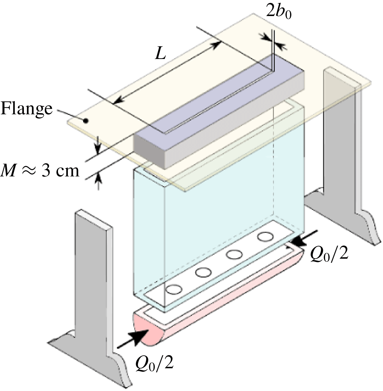
The principal design requirement was to achieve uniform source conditions. Several prototype nozzles were trialled until success was met with the design based on components shown in figure 16. Saline solution was pumped into the nozzle at its base through the two ends of a manifold. From there, the solution passed into a rectangular chamber through a row of sintered diffusers (shown as circles), whose purpose was to homogenise the flow. The slot was formed by securing two PVC sections a distance
 $2b_{0}$
apart. These sections, of depth
 $M\approx 3$
cm so that
 $M/b_{0}\approx 60$
, formed a rectangular duct which straightened the flow as it approached the exit plane of the slot. Surfaces were finely machined to provide a smooth lining, removing asperities that would otherwise trip the flow. Then, fixing spacers (of width
 $2\,b_{0}$
) between the two sections at either end reliably created a rectangular slot of length
 $L$
and width
 $2b_{0}$
. This assembled PVC section was, in turn, fixed onto the chamber. To provide ‘flush’ outlet conditions for the fountain (as opposed to re-entrant conditions), an acrylic flange was attached to the PVC section to form a horizontal plane. Finally, two supports allowed the nozzle to be levelled via adjustable feet. The remarkably good level of uniformity of the resulting release conditions is shown in figure 2 and discussed in § 3.
An advantage of the design proved to be its flexibility. Because the geometry of the slot was set by spacers, different geometries could be tested by installing different spacers. One caveat is that, if the slot length
 $L$
is much smaller than the length of the chamber, the slot acts as a contraction which bends the flow towards the centre. To mitigate this issue, in experiments with
 $L=150$
mm (set B, table 2) we inserted polystyrene blocks in regions of the chamber not below the slot and plugged the sintered holes beneath the blocks. These measures prevented the inward deflection very effectively.
Exploded view of the nozzle. A manifold of sintered holes feeds a plenum that precedes the slot.

Appendix B. Measurement and propagation of error
Estimates for the measurement error on parent variables are listed in table 2. The slot width was measured as
 $2\,b_{0}=1.00$
mm to within
 $0.05$
mm on a Vernier scale for both sets A and B, which led to a relative error on
 $b_{0}$
of
 $5\,\%$
. The volume flow rate
 $Q_{0}$
was measured on an ultrasonic flow meter, with fluctuations rarely exceeding
 $1\,\%$
(cf. the traces reported for the same apparatus in appendix A of Debugne & Hunt (Reference Debugne and Hunt2018)). The reduced gravity
 $g_{0}^{\prime }$
was inferred from the densitometer readings for
 $\unicode[STIX]{x1D70C}_{0}$
and
 $\unicode[STIX]{x1D70C}_{a}$
, accurate to within
 $5\times 10^{-4}~\text{g}~\text{cm}^{-3}$
. From these estimates, an upper bound for the error on the composite variables
 $w_{0}\equiv Q_{0}/(2b_{0}L)$
,
 $Fr_{0}\equiv w_{0}/\sqrt{b_{0}g_{0}^{\prime }}$
and
 $L/b_{0}$
was estimated according to the propagation rule (Taylor Reference Taylor1997):
 $q=X^{a}Y^{b}\Rightarrow \unicode[STIX]{x1D6FF}q/|q|=|a|\unicode[STIX]{x1D6FF}X/|X|+|b|\unicode[STIX]{x1D6FF}Y/|Y|$
. The results are given in table 4. Thus, the major contribution to the error comes from
 $b_{0}$
. It is not surprising that
 $b_{0}$
, whose absolute size is small, should give rise to relatively large errors. Nevertheless, the overall error is acceptable.
Error on
 $z_{v}$
arises both from inaccuracies in edge detection and from imperfect pixel-to-length calibration. We estimate the total error on
 $z_{v}$
as
 $\pm 2\,\%$
; based on a visual inspection (figure 3
a–c) this represents a conservative estimate.
Our identification of the frequencies is robust: by selecting the median of many frequencies calculated along
 $x$
or
 $y$
, we mitigate the risk of falsely retaining spurious frequencies. Except for a few experiments, for which we manually corrected the frequencies by counting bands such as in figure 13 or 20 and dividing the total count by the duration of the experiment, the retained frequencies should be regarded as precise. The remaining error is associated with the resolution in the frequency domain,
 $\unicode[STIX]{x0394}f=1/\unicode[STIX]{x0394}T$
. Assuming an error of
 $\pm 2\unicode[STIX]{x0394}f$
, relative errors on the frequencies never exceeded
 $2\,\%$
; the resulting (vertical) error bars were smaller than the size of the symbols in figures 10(a) and 11(a), and hence error bars were omitted.
The pre-factor
 $\unicode[STIX]{x1D6FE}_{v}$
in (4.5) differs by
 $19\,\%$
between sets A and B, approximately the same relative difference noted in pre-factor
 $\unicode[STIX]{x1D6FE}_{z}$
for the rise heights (4.3). The relative difference, however, is reversed: in set A,
 $\overline{\overline{z}}_{v}/b_{0}$
is larger by
 $19\,\%$
, whereas
 $f_{v}/(w_{0}/b_{0})$
is lower by
 $19\,\%$
. Of note is that the rise heights are normalised by
 $b_{0}$
, whilst the frequencies are normalised by a scale
 $\propto \,b_{0}^{-2}$
(on account that the mean source velocity is calculated as
 $w_{0}\cong Q_{0}/2b_{0}L$
). It therefore seems plausible that at least some of the discrepancy between measurement sets can be explained by differences in the accuracy to which
 $b_{0}$
could be read in either of the sets.
Upper bound estimate for the percentage error on composite variables.

Appendix C. Reynolds number effects on the rise heights
At low Froude numbers,
 $Re_{0}$
is known to influence both the rise height and the oscillatory behaviour of line fountains (Srinarayana et al.
Reference Srinarayana, Williamson, Armfield and Lin2010). Given the modest values for
 $Re_{0}$
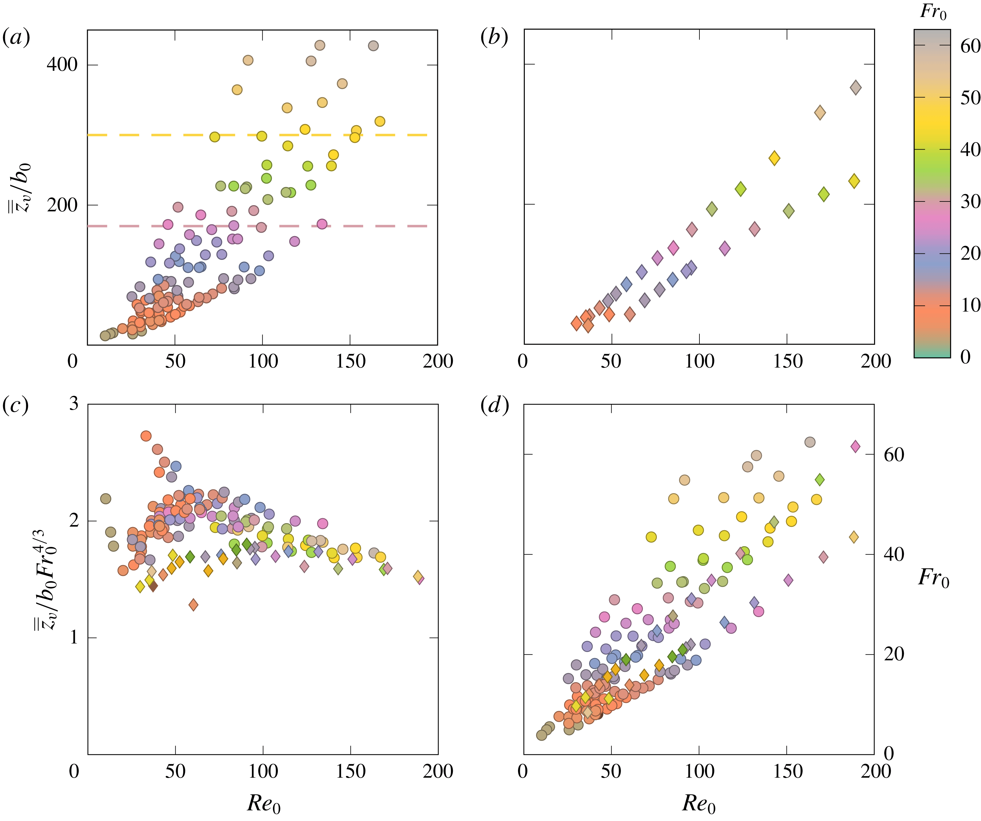
at which our fountains were formed (table 3), dependencies in our data on
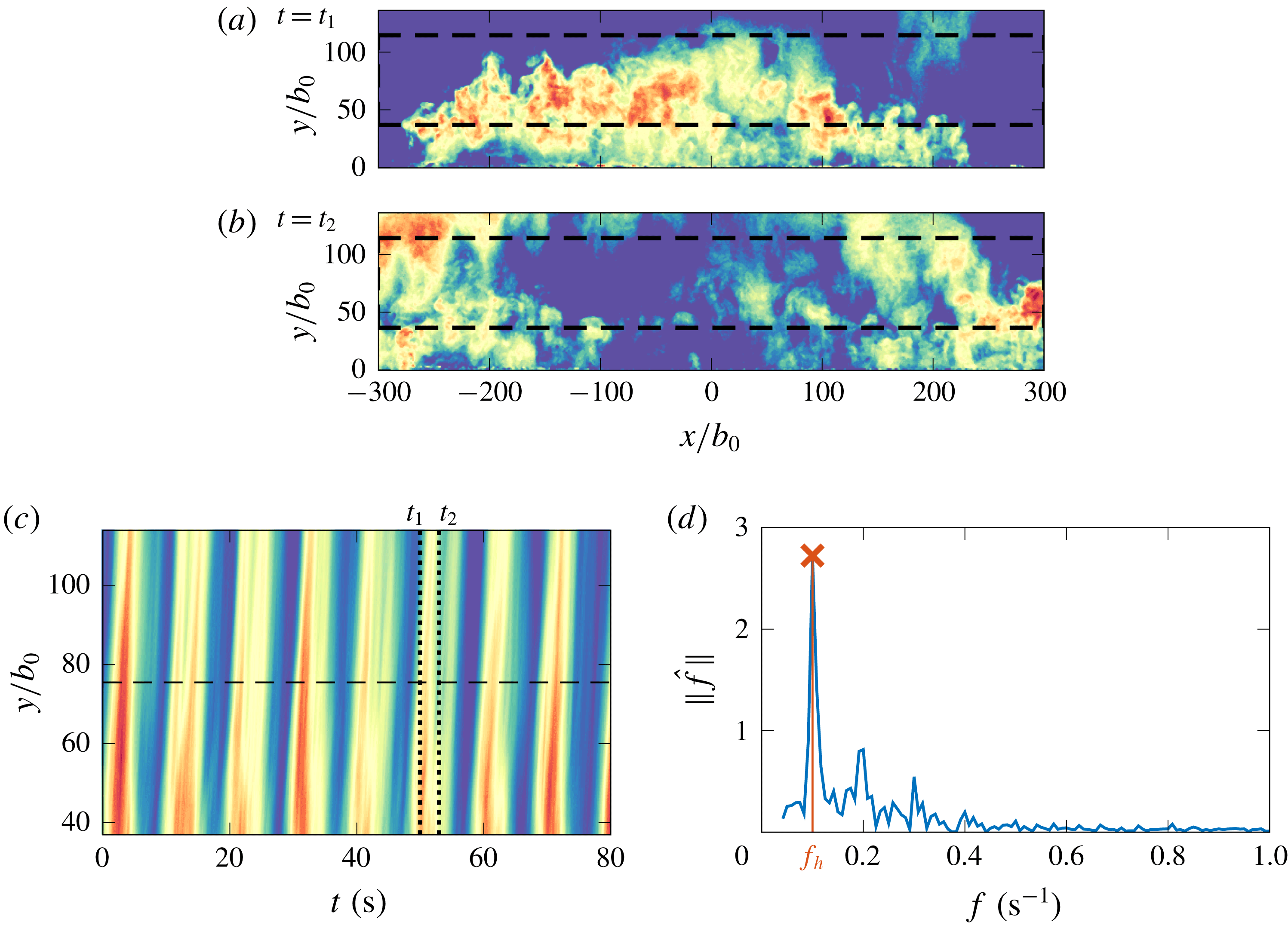
 $Re_{0}$
were explored despite the fountains always appearing highly turbulent. For a given slot, several experiments were repeated with fixed values for
 $Re_{0}$
and at different values for
 $Fr_{0}$
(by varying
 $g_{0}^{\prime }$
). Our data therefore contain measurements from experiments in which
 $Fr_{0}$
was varied for a nominally constant
 $Re_{0}$
, and vice versa. In figure 17 the experiment-averaged rise heights
 $\overline{\overline{z}}_{v}/b_{0}$
are shown plotted against
 $Re_{0}$
and the markers colour coded by
 $Fr_{0}$
. Specifically, the Froude numbers were divided into bins of width three units and each bin assigned a colour. Markers of a given colour therefore indicate closeness in
 $Fr_{0}$
. Likewise, horizontal lines denote lines of constant rise height, whereas vertical lines denote lines of constant
 $Re_{0}$
.
Experiment-averaged rise height
 $\overline{\overline{z}}_{v}/b_{0}$
against source Reynolds number
 $Re_{0}$
with markers colour coded for
 $Fr_{0}$
: (a) set A (
 $L/b_{0}=600$
) and (b) set B (
 $L/b_{0}=300$
). Horizontal dashed lines demark
 $\overline{\overline{z}}_{v}/b_{0}=300$
and
 $\overline{\overline{z}}_{v}/b_{0}=170$
. (c) Normalised rise height plotted against
 $Re_{0}$
. (d) Combinations of
 $Re_{0}$
and
 $Fr_{0}$
used in the experiments.

It is immediately apparent from figure 17 that same-coloured markers cluster around horizontal lines. Experiments run at similar values of
 $Fr_{0}$
achieve similar rise heights, with little sensitivity to the value of
 $Re_{0}$
. In figure 17(a), upper (yellow) and lower (mauve) horizontal lines were drawn at
 $\overline{\overline{z}}_{v}/b_{0}=300$
and
 $170$
, respectively. Rise heights adjacent to the upper and lower lines vary by
 $\pm 2\,\%$
and
 $\pm 3\,\%$
for Reynolds numbers varying by a factor of
 $2$
and
 $3$
, respectively; Froude numbers along the same lines lie within
 $\pm 6\,\%$
and
 $\pm 4\,\%$
of each other. Both the variations for
 $\overline{\overline{z}}_{v}/b_{0}$
and for
 $Fr_{0}$
are well within experimental error (
 $7$
% and
 $14\,\%$
, respectively, appendix B). We conclude that, for our experiments, the source Reynolds number does not have a significant effect on the rise heights.
The process of entrainment has a fundamental influence on the rise height of fountains (Hunt & Coffey Reference Hunt and Coffey2009). For the sake of argument, a formulation of an integral model for a two-dimensional line fountain (time and span averaged) could be used to understand the effect of entrainment on the rise height. Extending the top-hat formulation of Hunt & Debugne (Reference Hunt and Debugne2016) deduced for round fountains to the case of a non-flapping line fountain that is symmetric about each
 $(x=0,y,z)$
plane, the conservation equations for the volume flux per unit length,
 $Q_{L}=wb$
and specific momentum flux per unit length,
 $M_{L}=w^{2}b$
, can be deduced for the upflow
 $$\begin{eqnarray}\frac{\text{d}w_{u}b_{u}}{\text{d}z}=\unicode[STIX]{x1D6FC}_{f}\left(w_{u}-w_{c}\right),\quad \frac{\text{d}w_{u}^{2}b_{u}}{\text{d}z}=-(g_{u}^{\prime }-g_{c}^{\prime })b_{u}-\unicode[STIX]{x1D6FC}_{f}w_{u}w_{c},\end{eqnarray}$$
and counterflow
 $$\begin{eqnarray}\frac{\text{d}w_{c}b_{c}}{\text{d}z}=\unicode[STIX]{x1D6FC}_{f}\left(w_{c}-w_{u}\right),\quad \frac{\text{d}w_{c}^{2}b_{c}}{\text{d}z}=-g_{c}^{\prime }b_{c}-\unicode[STIX]{x1D6FC}_{f}w_{c}w_{u},\end{eqnarray}$$
where the subscripts
 $(.)_{u}$
and
 $(.)_{c}$
denote quantities associated with the upflow and counterflow, respectively, and
 $\unicode[STIX]{x1D6FC}_{f}$
is an entrainment coefficient. The results presented in this paper reveal a picture of the fountain which is significantly different from this integral model description and we proceed below in drawing comparisons with caution.
One might expect that the entrainment coefficient
 $\unicode[STIX]{x1D6FC}_{f}$
varies with
 $Re_{0}$
, in circumstances in which the flow is not fully turbulent, and with the local value of
 $Fr$
due to the adjustment behaviour of the upflow from the source (where
 $Fr=Fr_{0}$
) to the fountain top (where
 $Fr=0$
). By comparing our steady rise height measurement (i.e.
 $\overline{\overline{z}}_{v}/b_{0}~=~\unicode[STIX]{x1D6FE}_{z}Fr_{0}^{4/3}$
) with the height at which solutions to equations (C 1) and (C 2) become singular (cf. the approach of Kaye & Hunt Reference Kaye and Hunt2006 and Hunt & Debugne Reference Hunt and Debugne2016, but here neglecting fountain-top entrainment), a single representative value for the entrainment coefficient may be deduced, namely,
 $\unicode[STIX]{x1D6FC}_{f}=0.035\pm 0.014$
. One might also expect that flapping could alter entrainment. Observations reported herein, however, indicate that the rise height does not appear to alter in its power-law dependence between flapping regimes, an invariance suggestive of regimes underpinned by the same driving mechanism.
High wavenumber flapping. (a,b) Synchronous side views (left) and top views (right) of a fountain formed at
 $\{L,b_{0}\}=\{300,0.5\}$
mm and
 $Fr_{0}=5.5$
(
 $Re_{0}\approx 15$
). In the side views, the upper part of the fountain appears as a turquoise band; the lower part appears in red (i.e. darker), because of the relatively greater depth of dyed fluid. Images not to scale. (c) Contour map of the vertical fluctuations (cf. figure 13), with black dotted lines indicating the times at which images (a) and (b) were taken. Movie 8 available online.

Appendix D. Low-
$Fr_{0}$
line fountains

High wavenumber flapping. Fluorescence visualisation of the central section for
 $\{L,b_{0}\}=\{300,0.5\}$
mm and
 $Fr_{0}=6.1$
(
 $Re_{0}\approx 21$
). Images spaced at time intervals of
 $\unicode[STIX]{x0394}t=1.3$
s (
 $\cong 0.6~w_{0}/g_{0}^{\prime }$
). Movie 9 available online.

For certain combinations of
 $Fr_{0}$
and
 $L/b_{0}$
, we noted in § 3 that the flow was turbulent and non-uniform along the span, and exhibited a sinusoidal-like flapping motion comprising of one and a half winds (approximately). It will be shown in § 4.6 that different flapping patterns coincide with different ranges of
 $\overline{\overline{z}}_{v}/L$
, the ratio of rise height to slot length. Observations in § 3 pertain to turbulent fountains for which
 $\overline{\overline{z}}_{v}/L\gtrsim 0.05$
. Below, we briefly discuss the characteristics of fountains formed at
 $\overline{\overline{z}}_{v}/L\lesssim 0.05$
.
Figure 18(a,b) plots two representative side views together with the synchronous top views for a fountain produced at
 $L/b_{0}=600$
and
 $Fr_{0}=5.5$
(with
 $Re_{0}\approx 15$
), so that
 $\overline{\overline{z}}_{v}/L=0.029$
. The absence of fine-scale structures in figure 18(a,b) confirms that the flow is laminar. Individual parcels of fluid fluctuate vertically in the side views, forming localised crests at the fountain top. As these parcels collapse alternately to both sides of the centre plane, they produce a complex but regular oscillatory pattern, visible in the top views, comprising of circa eight wavelengths, i.e. considerably more than observed for
 $0.05\lesssim \overline{\overline{z}}_{v}/L\lesssim 0.30$
(e.g. figure 3
a). The intricacy of the pattern can be inferred from figure 18(c), where the deviations from the time-averaged rise height profile,
 $z_{v}(x,t)-\left\langle z_{v}\right\rangle _{t}(x)$
are plotted (cf. figure 13). By comparison with figure 13(a), it is clear that the scale of the fluctuations is finer in figure 18(c), and that the fluctuations are interspersed with a greater number of (local) troughs and crests. Interestingly, the location along the span of these troughs and crests does not appear to vary with time, which suggests the existence of persistent nodes in the oscillation.
Results similar to those shown in figure 18 were obtained for all experiments in which
 $\overline{\overline{z}}_{v}/L\lesssim 0.05$
. Whilst the exact oscillating patterns varied with
 $\overline{\overline{z}}_{v}/L$
, figure 18 gives a good indication of their level of intricacy. It is noteworthy that low values of
 $\overline{\overline{z}}_{v}/L$
could only be achieved at low values of
 $Re_{0}$
, such that the flow was systematically laminar or transitional. The weak (as opposed to ‘forced’) nature of these fountains is further reinforced in the LIF visualisation shown in figure 19 where lobes of dense fluid are shed to each side of the slot. In line with the investigations of Williamson et al. (Reference Williamson, Srinarayana, Armfield, McBain and Lin2008) and Srinarayana et al. (Reference Srinarayana, Williamson, Armfield and Lin2010), we therefore expect that the behaviour of such ‘weak’ high-source-aspect-ratio fountains should depend on both
 $\overline{\overline{z}}_{v}/L$
and
 $Re_{0}$
. Our focus herein lies on forced and turbulent line fountains, for which a subdivision according to
 $\overline{\overline{z}}_{v}/L$
alone appears promising (figure 14). Hence, we do not further pursue the analysis of laminar or transitional line fountains.
Illustration of ‘eddy counting’ applied to the top view (
 $L/b_{0}=600$
,
 $Fr_{0}=15.6$
). (a,b) Instantaneous images, 3 s apart (
 $\cong 0.3~w_{0}/g_{0}^{\prime }$
), of the upper half-plane
 $y\geqslant 0$
. Dashes delineate the windows, spanning
 $x\in [-L/2,L/2]$
and
 $y\in [0.5\,\overline{\overline{z}}_{v},1.5\,\overline{\overline{z}}_{v}]$
, over which each image is averaged (in
 $x$
) to produce (c). (c) The resulting time series is computed by repeating the averaging operation for every frame of the recording. Flapping events passing through the averaging windows leave bright, localised streaks. Dotted lines mark the times which correspond to (a) and (b). (d) Fourier transform of the luminosity levels along
 $y/b_{0}=75$
(dashed line, c). A distinct peak emerges at
 $f=f_{h}=0.1~\text{s}^{-1}$
, consistent with (c) where successive streaks are spaced approximately
 $1/f=10$
s apart.

Example of frequency analysis performed on the fluorescence visualisations (
 $L/b_{0}=600$
and
 $Fr_{0}=14.7$
). (a) A ‘Canny’ (Reference Canny1986) edge detection algorithm identifies the fountain outline (shown in magenta) and a three-point edge tracking records the peak height (●), and the peak lateral excursions (♦ and ▪) at heights exceeding 75 % of the peak height. (b) Patches formed by plotting the positions of the tracked points over a 140 s (
 $\cong 50\,w_{0}/g_{0}^{\prime }$
) experiment indicate the extent of vertical and lateral motions. (c) Signal of the vertical fluctuations and (d) the modulus of the Fourier coefficients
 $\Vert \hat{f}_{v}\Vert$
of this signal plotted in the frequency domain. (e) Signal of the lateral fluctuations and (f) the modulus of the Fourier coefficients
 $\Vert \hat{f}_{h}\Vert$
of this signal plotted in the frequency domain. In (c,e) dashed lines denote the mean values,
 $\overline{\unicode[STIX]{x1D6FF}z}_{v}$
and
 $\overline{\unicode[STIX]{x1D6FF}y}_{h}$
, respectively, of the peak amplitudes of the signals; dotted lines indicate two standard deviations either side of these means.

Appendix E. The eddy-counting approach
Figure 20 illustrates this approach in the context of line fountains. It relies on constructing, from a suite of frames, suitable time series in which large structures leave ‘traces’ that can be counted. Specifically, the
 $(y,t)$
-time series in figure 20(c) was constructed by averaging in
 $x$
, at every instant
 $t$
, an instantaneous image over a suitably chosen window (figure 20
a,b, black dashes). Thus, a flapping event passing over the window, when averaged in
 $x$
, will leave a ‘trace’ in figure 20(c) as dyed fountain fluid occupies a greater fraction of the window than the background does. Once the complete time series has been constructed for one experiment, the individual traces can be counted, as described above, or, alternatively, the frequency of the traces can be extracted directly through Fourier transforms (figure 20
d). The latter approach proved more reliable and easier to implement, hence we opted for Fourier transforms.
As an example of how the eddy-counting approach identifies the frequencies of the lateral fluctuations, we refer to figure 20. We intentionally chose a case of non-uniform flapping to highlight the robustness of the approach. In (a), captured at time
 $t=t_{1}$
, the fountain has begun to flap across the averaging window. As a result, a bright streak forms in time series (c) at time
 $t=t_{1}$
. In (b), captured at time
 $t=t_{2}$
, the fountain fluid has passed through the central section of the averaging window, but is emerging at the ends, where the flapping is phase shifted (§ 3). Nevertheless, the average brightness across the window decreases, hence the streak at time
 $t=t_{2}$
is dimmer. Because the brightest streaks are associated with the flapping of the (larger) central section only, its underlying frequency can be found through Fourier transforms. We demonstrate this point by applying a Fourier transform to the luminosity levels along
 $y/b_{0}=75$
in (c) (i.e. along the horizontal dashed line, chosen arbitrarily). The modulus of the resulting Fourier coefficients
 $\Vert \hat{f}\Vert$
is plotted in the frequency domain in (d). A clear peak emerges at
 $f=f_{h}=0.10~\text{s}^{-1}$
, which agrees closely with the time series (c), where bright streaks that mark flapping events are spaced approximately
 $1/f=10$
s apart. Therefore, we conclude that the approach successfully identifies the dominant flapping frequencies
 $f_{h}$
of line fountains.
Logarithmic plot of the root-mean-square velocities at the fountain top
 $w_{v}/w_{0}$
against
 $Fr_{0}$
. The line of best fit (see text) for
 $Fr_{0}\geqslant 10$
with slope
 $-2/3$
is shifted for ease of reading. Symbols as in figure 8.

Appendix F. Analysis of LIF experiments
Figure 21 illustrates the analysis conducted on the LIF images of the fountain centre plane to extract vertical and horizontal frequencies and the extent of the lateral excursions. A ‘three-point’ tracking scheme (figure 21 a,b) was developed to detect, from each instantaneous fountain outline, the peak rise height and the peak lateral excursions, the latter identified above 75 % of the peak height to avoid detecting features in the lateral currents. The frequencies corresponding to the peak Fourier coefficient of the transformed signals (figure 21 c–f) are shown by the dark red shaded symbols in figures 10 and 11. Evidently, there is generally good agreement between the frequencies, both vertical and horizontal, identified by the LIF and the dye-attenuation approaches.
Appendix G. Velocities at the fountain top
On dimensional grounds, the vertical velocities in line fountains are expected to scale as
 $w\propto w_{0}Fr_{0}^{-2/3}$
(e.g. van den Bremer & Hunt Reference van den Bremer and Hunt2014a
). In § 4.3, we inferred this scaling for the velocities at the fountain top,
 $w_{v}$
, by combining the fluctuation amplitude
 $\unicode[STIX]{x1D6FF}z_{v}$
and frequency
 $f_{v}$
as
 $w_{v}\sim \unicode[STIX]{x1D6FF}z_{v}f_{v}$
. In what follows, we estimate
 $w_{v}$
directly from our rise height data.
To proceed we differentiate, in time, the signal
 $z_{v}(x,t)$
at every
 $x$
-location along the slot. Then, we screen out any (rare) outliers by excluding gradients whose magnitude lies within three standard deviations above or below the mean gradient. Finally, an estimate for
 $w_{v}$
is obtained as the root-mean-square of the screened gradients,
 $(\text{d}z_{v}/\text{d}t)_{rms}$
, averaged over all
 $x$
. The resulting velocities
 $w_{v}$
, normalised by
 $w_{0}$
, are plotted against
 $Fr_{0}$
in figure 22. Also plotted is a line of best fit,
 $w_{v}/w_{0}=0.540Fr_{0}^{-2/3}$
. The fit is good for relatively forced releases,
 $Fr_{0}\gtrsim 10$
, in accord with the theoretical scaling.