1 Introduction
1.1 Taylor–Couette flows
Azimuthal flow between two concentric rotating cylinders, or Taylor–Couette (TC) flow, is a seminal fluid dynamic platform used in understanding the effects of hydrodynamics on complex fluids and processes (Fardin, Perge & Taberlet Reference Fardin, Perge and Taberlet2014). It is well known for Newtonian fluids that beyond a critical speed of inner cylinder rotation, the flow transitions from unidirectional azimuthal flow (Couette flow, CF) to stationary toroidal vortices (laminar Taylor vortex, LTV), found initially by Taylor (Reference Taylor1923). As the inner cylinder speed further increases, the vortices evolve further at critical points, gaining a temporal frequency (dominant frequency of the travelling wave (or azimuthal frequency) (laminar wavy vortex, LWV), multiple temporal frequencies (modulated wave vortices, MWV) and turbulent features (turbulent wavy vortex, TWV and turbulent Taylor vortex, TTV) (Andereck, Liu & Swinney Reference Andereck, Liu and Swinney1986; Dutcher & Muller Reference Dutcher and Muller2009). The cascade of flow instabilities and wide variety of flow states have been used to enhance the fundamental understanding between flow field and complex processes such as polymer–clay flocculation (Coufort, Bouyer & Liné Reference Coufort, Bouyer and Liné2005), drag reduction (van den Berg et al. Reference van den Berg, Doering, Lohse and Lathrop2003; Dutcher & Muller Reference Dutcher and Muller2011), heterogeneous versus homogenous catalysis (Sczechowski, Koval & Noble Reference Sczechowski, Koval and Noble1995) and liquid–liquid mixing (Nemri, Charton & Climent Reference Nemri, Charton and Climent2016).
TC flow dynamics are typically characterized by the Reynolds number (
 $Re$
), based on the gap width,
 $d$
, cylinder speed (primarily the inner cylinder speed),
 $\unicode[STIX]{x1D6FA}_{i}r_{i}$
, and kinematic viscosity,
 $\unicode[STIX]{x1D708}$
. The Reynolds number is typically defined as
 $$\begin{eqnarray}\displaystyle Re=\unicode[STIX]{x1D6FA}_{i}r_{i}d/\unicode[STIX]{x1D708}. & & \displaystyle\end{eqnarray}$$
Another important parameter is the radius ratio,
 $\unicode[STIX]{x1D702}$
, defined as the ratio of the inner and outer cylinder radii, which captures the relative range of curvature of the fluid streamlines (Dutcher & Muller Reference Dutcher and Muller2007), and is fixed within the narrow gap regime in the current study. Finally, the aspect ratio in this study is within the large aspect ratio regime to avoid end effects.
TC cells offer the advantages of optical access, well-defined flows with limited spatial and temporal variation of hydrodynamic conditions compared to other geometries, and a rich cascade of different flow states that offer a range of hydrodynamic conditions, both laminar and turbulent. These TC cell advantages improve process performance in a variety of applications, including polymerization (Kataoka et al. Reference Kataoka, Ohmura, Kouzu, Simamura and Okubo1995), composite pigment synthesis (Kim et al. Reference Kim, Park, Lee, Kim, Kim, Kwon and Kim2014), photocatalysis (Sczechowski et al. Reference Sczechowski, Koval and Noble1995; Dutta & Ray Reference Dutta and Ray2004), food processing (Krintiras et al. Reference Krintiras, Gadea Diaz, van der Goot, Stankiewicz and Stefanidis2016), emulsion generation (Park et al. Reference Park, Forney, Kim and Skelland2004), bioreactors (Haut et al. Reference Haut, Ben Amor, Coulon, Jacquet and Halloin2003; Ramezani et al. Reference Ramezani, Kong, Gao, Olsen and Vigil2015), extraction (Baier & Graham Reference Baier and Graham2000; Ahmad et al. Reference Ahmad, Kusumastuti, Shah Buddin, Derek and Ooi2014) and medical applications (Beaudoin & Jaffrin Reference Beaudoin and Jaffrin1989). However, these process improvements have largely only been demonstrated at the laboratory scale and there is limited commercial application of TC cells. Additionally, there is still only a small operational parameter space explored for multiphase TC flows. Due to mechanical complexity, injection of a second fluid into the annulus during rotation has been traditionally accomplished through single access points in a stationary outer cylinder or through the top of the annulus, restricting mixing performance and analysis.
1.1.1 Mixing in Taylor–Couette flows
There have been several studies examining mixing and mass transfer (Ohmura et al. Reference Ohmura, Kataoka, Shibata and Makino1997, Reference Ohmura, Makino, Motomura, Shibata and Kataoka1998; Dusting & Balabani Reference Dusting and Balabani2009; Nemri et al. Reference Nemri, Climent, Charton, Lanoë and Ode2013, Reference Nemri, Cazin, Charton and Climent2014, Reference Nemri, Charton and Climent2016) as well as momentum transport (van den Berg et al. Reference van den Berg, Doering, Lohse and Lathrop2003; Dubrulle et al. Reference Dubrulle, Dauchot, Daviaud, Longaretti, Richard and Zahn2005; Eckhardt, Grossmann & Lohse Reference Eckhardt, Grossmann and Lohse2007) in TC flows. Enhanced mass transport in TC flow is attributed to advective transport from the vortex structures with two different transport mechanisms: inter- and intra-vortex transport. The dispersion coefficients are several orders of magnitude higher than molecular diffusion coefficients, indicating the importance of the controlled mixing available in TC flow. Different techniques have been used to quantify mass transfer, including residence time distribution measurements (Ohmura et al. Reference Ohmura, Makino, Motomura, Shibata and Kataoka1998; Nemri et al. Reference Nemri, Climent, Charton, Lanoë and Ode2013, Reference Nemri, Charton and Climent2016) and laser induced fluorescence (LIF) techniques (Dusting & Balabani Reference Dusting and Balabani2009; Nemri et al. Reference Nemri, Cazin, Charton and Climent2014, Reference Nemri, Charton and Climent2016) to generate spatial and temporal profiles. While residence time distribution measurements, consisting of measuring concentration time profiles at multiple individual locations axially along the annulus, offer experimental simplicity, only a limited number of vortices can be examined at one time and no spatial inhomogeneities can be observed. In contrast, during LIF and similar techniques, the entire spatial concentration profile can be captured over time, increasing the detail that can be observed. For example, a study by Dusting & Balabani (Reference Dusting and Balabani2009) revealed different mixing processes within different spatial regions inside a single vortex in LTV flow state. A similar phenomenon is observed in the LWV structure, where a poorly mixed region in the core of the vortex is observed (Nemri et al. Reference Nemri, Cazin, Charton and Climent2014).
A few different models have been used to analyse the mass transport behaviour in TC flows, summarized by Nemri and co-workers (Reference Nemri, Charton and Climent2016). One of the first models proposed by Kataoka & Takigawa (Reference Kataoka and Takigawa1981) treated each unitary vortex pair as a well-mixed reactor; thus mass transport was modelled as intermixing between a series of continuous stirred tank reactors, yielding a single axial mass transfer coefficient. Since several studies have observed different regimes of mass transfer within a vortex, a two-zone model has been used (Nemri et al. Reference Nemri, Cazin, Charton and Climent2014) where the ‘unmixed core’ is treated as a separate mass transfer zone. The model can be pictured as treating each vortex as two well-mixed reactors, one inside the other, yielding two mass transfer coefficients, one between adjacent vortices and one between zones inside individual vortices. However, defining the spatial boundaries of these two zones inside the LWV is non-trivial due to vortex axial motion.
While many studies of mixing and mass transfer in TC flows exist, previous studies examined one or two flow states over a narrow range of
 $Re$
. A variety of correlations of mass transfer with
 $Re$
have been determined (Ohmura et al.
Reference Ohmura, Kataoka, Shibata and Makino1997, Reference Ohmura, Makino, Motomura, Shibata and Kataoka1998; Dusting & Balabani Reference Dusting and Balabani2009; Nemri et al.
Reference Nemri, Cazin, Charton and Climent2014, Reference Nemri, Charton and Climent2016), but correlations are often only for single flow state regimes and there tends to be little consensus in the results. Adding to the intricacy, studies have reported multiple mass transfer coefficients for a given
 $Re$
, depending on the ramp protocol used to form the vortex structure (Nemri et al.
Reference Nemri, Charton and Climent2016).
Mechanical restrictions from the TC geometry have constrained previous studies to use single injection locations, either at the top of the annulus (Dusting & Balabani Reference Dusting and Balabani2009) or through holes in the outer cylinder (Nemri et al. Reference Nemri, Climent, Charton, Lanoë and Ode2013, Reference Nemri, Cazin, Charton and Climent2014, Reference Nemri, Charton and Climent2016). Often, a capillary is inserted in the annulus from the external hole to inject in the centre of a particular vortex (Nemri et al. Reference Nemri, Charton and Climent2016). While yielding precise control over injection location, the presence of the capillary in the annulus can locally alter the flow profile. Indeed, the prior studies (Nemri et al. Reference Nemri, Cazin, Charton and Climent2014, Reference Nemri, Charton and Climent2016) take care to minimize flow disturbances and show evidence for a different rate of mass transfer between the inflow and outflow boundaries of the vortices. However, this interesting asymmetric behaviour may be potentially due to the presence of a capillary through only one of the flow boundaries. Therefore, mass transport without modification of the annulus geometry is needed to confirm the different inflow and outflow mass transfer behaviour.
Additionally, the single injection location restricts the amount of fluid that can be injected without disrupting the vortex structure. The short pulse of mass at a single point results in concentration profiles measured with LIF techniques being azimuthally periodic, limiting temporal data resolution to once per vortex per rotation period and mass transfer occurring in both the axial and azimuthal directions, complicating the mass transfer analysis (Nemri et al. Reference Nemri, Cazin, Charton and Climent2014). To address this, in order to determine a diffusion coefficient, a volume averaged concentration per vortex is needed to remove the azimuthal gradients present from the short, pulsed injections (Nemri et al. Reference Nemri, Climent, Charton, Lanoë and Ode2013, Reference Nemri, Cazin, Charton and Climent2014, Reference Nemri, Charton and Climent2016). However, this averaging method convolutes azimuthal mass transport with axial mass transport and decreases the temporal resolution of the concentration measurements. Modified injection mechanisms from multiple azimuthal positions at a given axial position could be used to remove the azimuthal concentration gradient, decreasing the complexity of measuring axial mass transport. In addition, expanded fields of view can be used to study longer range mass transport behaviour.
1.2 Improved Taylor–Couette geometry for mixing studies
A new, modified TC cell design has been recently described and characterized that incorporates 16 injection ports evenly distributed axially (10 cm spacing) and azimuthally (
 $90^{\circ }$
spacing) into the inner cylinder, allowing for injection of large volumes during co- and counter-rotation (Wilkinson & Dutcher Reference Wilkinson and Dutcher2017). Most importantly, the modified design’s injection system is non-intrusive in the annulus, unlike systems using capillaries or syringes inserted into the annulus. The flush ports do not alter the flow profile, leaving the vortex structures undisturbed. Additionally, since the injection ports are located along the inner cylinder, the injection ports are moving azimuthally during injection, spatially distributing the injection fluid. This design has been shown to not alter the flow profile compared to traditional TC cell designs. Because the vortex structures are not disturbed by the injection mechanism itself, this design is ideal for observation of multi-vortex mass transport.
This is the first study that explicitly considers vortex stability to large volume injection and vortex stability during mass transport. Vortex stability is an important parameter because the process applications of interest often require large volumes of solution to be mixed. If the vortex structure is lost due to injection, the mass transfer process changes. When vortices reform, dislocations or a new vortex state may form, altering the mass transport. Even when a vortex flow state is stable to injections, the resulting axial flow can cause axial motion of the vortices that result in bulk transport of mass, rather than inter-vortex transport, further complicating mass transfer analysis.
In the present study, large volume injections (up to 13 % of annulus volume) were explored to study the stability of four different vortex structures (LTV, LWV, TWV, TTV), spanning two orders of magnitude of
 $Re$
. Injection conditions vary in both total amount and rate of injection. Dispersion coefficients were experimentally measured for the vortex structures under stable injection conditions tracking the temporal evolution of concentration within more than seven individual vortices. A non-dimensional stability criterion was then generated to define the stable operational space for injection conditions with different vortex structures.
2 Materials and methods
2.1 Equipment and materials
The Taylor–Couette cell used here is a modified TC cell design that incorporates 16 injection ports along the inner cylinder for non-intrusive injection of one fluid into another during operation. The complete details of the recent design have been described and characterized elsewhere (Wilkinson & Dutcher Reference Wilkinson and Dutcher2017). The inner cylinder is anodized aluminium (
 $d_{i}=13.54\pm 0.01~\text{cm}$
) and the outer cylinder is borosilicate glass (
 $d_{o}=15.20\pm 0.01~\text{cm}$
). The annulus gap axial height is 51 cm and the gap radial width is 0.84 cm. The radius ratio is 0.89 and the gap to height (aspect) ratio is 60. The working volume of fluid within the annulus is
 ${\sim}$
1.8 l. The top and bottom of the annulus are fixed to the outer cylinders and are stationary in the experiments done here. Further details and schematics on the end caps can be found in an earlier publication (Wilkinson & Dutcher Reference Wilkinson and Dutcher2017, figure 2). Additionally, fluid is removed through the perforations in the top cap of the cylinder during injections.
Each cylinder is driven by a stepper motor (Applied Motion Products HT34-497 2 phase stepper motor with a STAC5-S-E120 controller) with a
 $7:1$
gear reducer. The minimum speed change of each cylinder is
 $385.8~\unicode[STIX]{x03BC}\text{Hz}$
. Each injection port has a check valve with a 10 psi crack pressure and a flow restrictor to normalize flow between injection ports. This injection assembly provides consistent injections and the variation between injection rows is less than 7 % (Wilkinson & Dutcher Reference Wilkinson and Dutcher2017).
A Basler Ace camera (
 $1280\times 1024$
, 50 frames per second) is used for video capture with two different light sources. For vortex stability experiments, a LED light strip, equipped with a diffuser (Metaphase 19 in. Exo2 Light), aligned axially with the cell, provides consistent lighting along the entire height of the annulus. The LED orientation provides a view of the
 $\unicode[STIX]{x1D703}$
–
 $z$
plane of the vortex. For mass transfer experiments, a laser diode is used (Thorlabs, 450 nm, 1600 mW max) along with a laser light sheet generator optic to create a light sheet that is oriented normal to the surface of the inner cylinder. This orientation provides a view of the
 $r$
–
 $z$
plane of the vortex.
All water used was distilled water. Kalliroscope rheoscopic fluid was purchased from VWR and used as received. The density of the
 $9:1$
(by volume) distilled water : Kalliroscope solution used had a measured density of
 $994.6\pm 1.1~\text{kg}~\text{m}^{-3}$
. The viscosity was measured to be
 $1.006\times 10^{-6}~\text{m}^{2}~\text{s}^{-1}$
. The density of the distilled water used here was
 $995.1\pm 0.6~\text{kg}~\text{m}^{-3}$
and the density of stock Kalliroscope was measured to be
 $996.8\pm 1.6~\text{kg}~\text{m}^{-3}$
.
2.2 Injection flow rate calibration
The flow rates explored during the initial device characterization (Wilkinson & Dutcher Reference Wilkinson and Dutcher2017) only reached 30 psi drive pressures, reaching
 $5.9~\text{g}~\text{s}^{-1}$
flow rates with distilled water. Higher drive pressures were explored here and the flow rates from these pressures were measured using three solutions: (i) distilled water, (ii)
 $9:1$
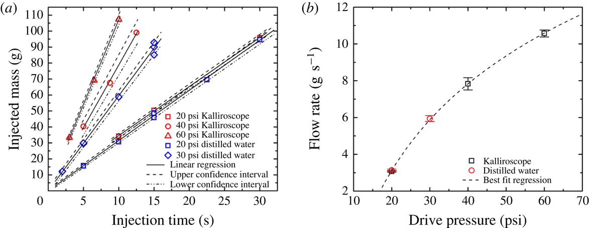
distilled water : Kalliroscope and (iii) undiluted Kalliroscope solutions. All solutions were found to have the same injection flow rate for a given drive pressure. The calibration to higher drive pressures was performed following the same calibration process for lower drive pressures described in detail previously (Wilkinson & Dutcher Reference Wilkinson and Dutcher2017). The inner cylinder was removed from the outer cylinder and the three-dimensional printed contour match covers were removed to aid in sample collection. Scintillation vials were attached to the end of each injection port and fluid sample masses were measured for a variety of injection times at the desired injection pressure. Figure 1(a) shows the individual flow rate calibrations with 95 % confidence intervals. Figure 1(b) shows the total injection mass flow rate as a function of drive pressure. All experiments reported here were conducted within the calibrated range of 20–60 psi.
Injection mass flow rate calibration with injection pressure. (a) Individual calibration experiments for each drive pressure for both distilled water and Kalliroscope solutions. The red symbols correspond to Kalliroscope solutions and the blue symbols correspond to distilled water solutions. The solid lines represent the best fit linear regression used to quantify the flow rates shown in (b). The dashed lines are the 95 % confidence intervals for each linear regression. (b) The total mass flow rate through the injection system as a function of drive pressure for various pressures used to calculate the injected mass in further experiments. The equation for the regression is flow rate
 $=$
6.79 ln(drive pressure
 $/$
1 psi) 17.23, with units as shown in (b).

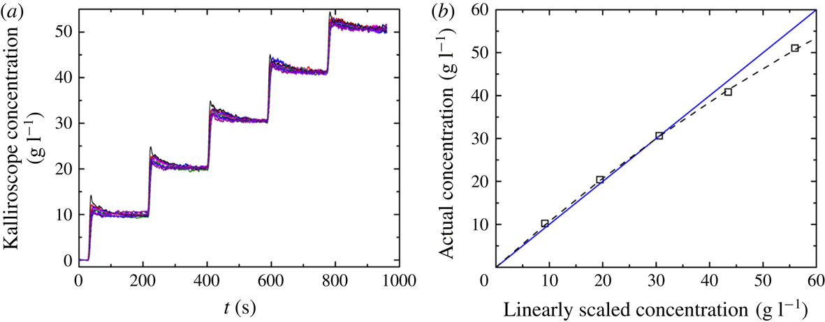
(a) Concentration profiles for several vortices of repeated 20 g (1.1 % annulus) Kalliroscope solution injections in the TTV structure. (b) Final average Kalliroscope concentration calibration curve generated from the repeated 20 g (1.1 % annulus) Kalliroscope injection used to correct the linear scaling. The solid blue line corresponds to
 $y=x$
. The dashed black line is the best fit quadratic calibration curve used to correct the linearly scaled concentration data.

2.3 Vortex stability experiments
For experiments assessing vortex stability to radial injection, the annulus was filled with a 9:1 water : Kalliroscope solution and the same mixture was injected through all of the inner cylinder injection ports. Injection of like fluids eliminates gradients in fluid properties, such as Kalliroscope concentration. The desired vortex state was established in the annulus prior to injection. Care was taken to eliminate any discontinuities, also known as dislocations (Dutcher & Muller Reference Dutcher and Muller2009), in the vortex structure. These discontinuities give the appearance of two vortices merging and separating as they rotate and are an artefact that should be avoided when doing stability and mass transfer studies. For each vortex structure, a motor control script was created to control the inner cylinder speed to create the vortex structure reproducibly. In particular for the laminar wavy states, higher
 $Re$
flow states were first established, and then the inner cylinder motor speed was decreased. The motor scripts were used to generate the same vortex structures observed from equilibrium ramps (Dutcher & Muller Reference Dutcher and Muller2009) quickly and consistently. Similar techniques of motor ramping scripts for fast and consistent vortex generation have been used previously (Nemri et al.
Reference Nemri, Climent, Charton, Lanoë and Ode2013). Once the vortex structure was established, a video was taken, starting 30 s prior to injection, of the entire length of the annulus to capture the behaviour of all vortices. The resultant video was used to generate the space–time plots and subsequent Fourier transforms for analysis and characterization of flow stabilities, in a process described previously (Dutcher & Muller Reference Dutcher and Muller2009; Wilkinson & Dutcher Reference Wilkinson and Dutcher2017).
2.4 Mass transfer experiments
For experiments measuring vortex mass transfer, the annulus was loaded with distilled water and undiluted Kalliroscope solution was injected through all of the injection ports into the annulus. While Kalliroscope contains particulates, making measurement of molecular diffusion impossible, advection is far more important than diffusion in TC flow since the measured dispersion coefficients are many orders of magnitude greater than molecular diffusion coefficients. Similar to the vortex stability experiments, the desired flow state was initially established prior to injection. Once the motor control script was completed, a video of the annulus between the fourth and third injection port rows was started 30 s prior to injection. The field of view was restricted to that between two ports to increase spatial resolution. For the LTV and TTV vortex states, the boundaries of the vortices were determined by plotting the pixel intensity profile in the axial direction. The pixel intensity drops at each vortex boundary and could be used to identify the boundary locations. An example image showing vortex locations is shown in supplementary figure S1 available online at https://doi.org/10.1017/jfm.2018.596. However, this technique does not work for the LWV and TWV flow states as the boundary moves axially and the decrease in pixel intensity is no longer present. Instead, the midpoint of each azimuthal wave was identified visually, and the average axial location was used. Time-dependent spatial variations in Kalliroscope concentration after injection was used to determine the mass transport coefficients, described below.
2.5 Intensity to concentration calibration
The concentration of Kalliroscope is measured by quantifying the intensity of light locally reflected by the Kalliroscope solids in solution. The calibration used here was to check the validity of linear scaling over the large range of Kalliroscope used in this study. Additionally, the calibration was done in the TC cell under experimentally relevant conditions to account for scattering from Kalliroscope out of the plane of the light sheet. A shortened explanation of the method is presented here, with the expanded version included in the supplementary information. The pixel intensity of each vortex area is averaged, producing a single concentration per vortex. A linear scaling is initially used, but a quadratic equation is used to correct for multiple scattering due to the relatively large concentrations of Kalliroscope. The intensity is first linearly scaled to concentration per vortex using the following equation:
 $$\begin{eqnarray}\displaystyle C=\frac{I-I_{o}}{I_{f}-I_{o}}\times \frac{m}{V_{o}+m/\unicode[STIX]{x1D70C}}, & & \displaystyle\end{eqnarray}$$
where
 $C$
is the concentration of Kalliroscope solution
 $(\text{g}~\text{l}^{-1})$
,
 $I$
is the instantaneous average pixel intensity,
 $I_{o}$
is the zero concentration (pre-injection) intensity,
 $I_{f}$
is the final concentration intensity,
 $m$
is the mass of Kalliroscope injected
 $(g)$
and
 $\unicode[STIX]{x1D70C}$
is the density of the Kalliroscope solution, which was measured to be
 $994.6\pm 1.1~(\text{kg}~\text{m}^{-3})$
.
 $V_{o}$
is the initial volume of distilled water in the annulus, equal to 1.8 l.
Because relatively large volume injections are explored here, the intensity to concentration profile is not necessarily linear with concentration. To account for this nonlinearity an injection of 20 g Kalliroscope in the TTV structure (
 $Re=6510$
,
 $v_{cylinder}=12~\text{cm}~\text{s}^{-1}$
) was repeated a total of five times with 3 min of time in between to allow for the concentrations in each vortex to equilibrate, shown in figure 2(a). The different coloured lines in figure 2(a) are the different individual vortices between the injection port rows 3 and 4. The concentration in each vortex at the end of the 3 min equilibration time between injections is compared to the expected concentration in the annulus. A regression was then performed to convert the linearly scaled concentration to the expected concentration, shown in figure 2(b), resulting in the following best fit quadratic scaling:
 $$\begin{eqnarray}\displaystyle C_{scaled}=-0.003613C^{2}+1.108C, & & \displaystyle\end{eqnarray}$$
where
 $C$
is the linearly scaled concentration of Kalliroscope from above and
 $C_{scaled}$
is the properly scaled Kalliroscope concentration (
 $\text{g}~\text{l}^{-1}$
), removing the effect of secondary scattering. The results of this scaling, shown in figure 2(b), primarily only affect Kalliroscope concentrations above
 $35~\text{g}~\text{l}^{-1}$
, where deviation from the
 $1:1$
scaling is apparent. The calibration at high loadings is important in the lower
 $Re$
vortex structures, such as the TWV, where the concentration of Kalliroscope in the vortices near the injection ports can be high.
2.5.1 Mass transfer coefficient analysis
Once time profiles of Kalliroscope concentration per vortex were constructed, regression of the intermixing coefficient can begin. An analysis procedure like that of Ohmura and co-workers (Reference Ohmura, Kataoka, Shibata and Makino1997) is used. The key difference here is that the analysis is per vortex, rather than per unitary vortex pair, as in Ohmura et al. (Reference Ohmura, Kataoka, Shibata and Makino1997). For the analysis, each vortex is treated as an individual well-mixed reactor. The spatial concentration of Kalliroscope in each vortex was averaged to create a single concentration per vortex for each frame. Therefore, the analysis only captures mass transport between vortices across the interfacial area between adjacent vortices. The mass balance for the
 $n$
th vortex is defined by
 $$\begin{eqnarray}\displaystyle V_{n}\frac{\unicode[STIX]{x2202}C_{n}}{\unicode[STIX]{x2202}t}=kS(C_{n-1}-2C_{n}+C_{n+1}), & & \displaystyle\end{eqnarray}$$
where
 $C_{n}$
is the concentration of the
 $n$
th vortex (the vortex of interest) and subscripts
 $n+1$
and
 $n-1$
correspond to adjacent vortices.
 $V_{n}$
is the volume of the
 $n$
th vortex
 $[\unicode[STIX]{x03C0}(r_{o}^{2}-r_{i}^{2})L_{n}]$
,
 $S$
is the interfacial area between vortices
 $[\unicode[STIX]{x03C0}(r_{o}^{2}-r_{i}^{2})]$
and
 $k$
is the intermixing coefficient.
Nemri et al. (Reference Nemri, Cazin, Charton and Climent2014) observed a difference in the mass transfer at the inflow and outflow boundaries in the LTV and LWV flow states. A modification was made to (2.3) to test for different behaviour at the inflow ‘in’ and outflow ‘out’ boundaries, resulting in the following:
 $$\begin{eqnarray}\displaystyle V_{n}\frac{\unicode[STIX]{x2202}C_{n}}{\unicode[STIX]{x2202}t}=k_{in}S(C_{n-1}-C_{n})-k_{out}S(C_{n}-C_{n+1}). & & \displaystyle\end{eqnarray}$$
Equation (2.4) is used for every other vortex and
 $k_{in}$
and
 $k_{out}$
are switched for the remaining vortices.
To determine the best fit
 $k$
for each experiment, the fsolve function in Matlab was used to minimize the mean square error between the predicted vortex concentrations over time and the measured values. The experimentally measured concentrations in the vortices located just above the fourth row injection port and the vortex located just below the third row injection port were used as boundary conditions in the determination of
 $k$
.
3 Results and discussion
3.1 Mass transfer
First, the intermixing coefficients in (2.3) and (2.4) were determined. Because stock Kalliroscope solution is injected into distilled water for these experiments, the solution properties, and thus
 $Re$
, change slightly over the course of the experiment. The
 $Re$
used to define each experiment is based on the final solution conditions and is thus the lowest value over the course of each experiment. As the 16 injection ports are located along the inner cylinder, there are minimal azimuthal concentration gradients present, making the primary concentration gradient in the axial direction. The azimuthal gradient is only observable in the lowest vortex state, the LTV, but the LTV is so weak that even the 50 g (2.7 % by volume of annulus ‘% annulus’, 16 s) injection at 20 psi (
 $3.1~\text{g}~\text{s}^{-1}$
 $0.32~\text{m}~\text{s}^{-1}$
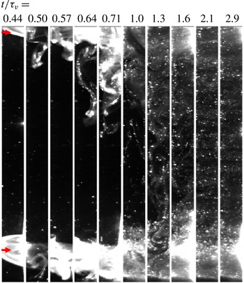
) of stock Kalliroscope into distilled water was enough to disrupt the vortex structure. The disruption comes from both the radial injection, discussed later, and the slight density difference between the stock Kalliroscope solution and distilled water. Future studies could potentially increase the viscosity of the solutions to circumvent the issues observed here. An example of this disruption can be seen in figure 3, where between 31 and 50 s, there is a stream of Kalliroscope that falls from the injection ports at the top of the images. Figure 3 also shows an azimuthal concentration gradient, as denoted by the change in intensity between the panels showing 31, 35 and 40 s. Because of this disruption of the vortex structure, an intermixing coefficient was not experimentally measured for the LTV. Instead, the regressed trend of the intermixing coefficient was extrapolated to determine a value for the LTV structure. Increasing the viscosity of the fluid in the annulus could potentially stabilize the vortex, but is beyond the scope of the current study.
Mass transfer results for the LTV structure (
 $Re=146$
,
 $v_{cylinder}=1.7~\text{cm}~\text{s}^{-1}$
,
 $\unicode[STIX]{x1D6FA}_{cylinder}=0.041~\text{Hz}$
) for a 20 psi (
 $3.1~\text{g}~\text{s}^{-1}$
,
 $0.32~\text{m}~\text{s}^{-1}$
) 50 g injection (2.7 % annulus,
 $t_{inject}=16~\text{s}$
). Snapshots of the annulus between injection port rows 3 and 4 after injection illustrating the spatial concentration evolution. The numbers at the top of panel represent the dimensionless time,
 $t/\unicode[STIX]{x1D70F}_{\unicode[STIX]{x1D708}}$
(
 $\unicode[STIX]{x1D70F}_{\unicode[STIX]{x1D708}}=d^{2}/\unicode[STIX]{x1D708}$
), of each panel. The red arrows indicate the axial location of the injection port rows 3 and 4, which are 10 cm apart.

Each injection value (20 (1.1 % annulus), 50 (2.7 % annulus), and 100 g (5.5 % annulus)) at 20 psi (
 $3.1~\text{g}~\text{s}^{-1}$
,
 $0.32~\text{m}~\text{s}^{-1}$
) was explored at a single
 $Re$
value for each vortex structure (LTV, LWV, TWV and TTV) and the variation of the regressed intermixing coefficients with injected mass was less than 10 %. This variation is within the variation observed from replicates at
 $Re=2083$
,
 $v_{cylinder}=25~\text{cm}~\text{s}^{-1}$
(TWV) and
 $Re=6510$
,
 $v_{cylinder}$
(surface velocity of the inner cylinder)
 $=77~\text{cm}~\text{s}^{-1}$
,
 $\unicode[STIX]{x1D6FA}_{cylinder}=1.8~\text{Hz}$
(TTV). Because all the injection mass values produced the same results, only 50 g (2.7 % annulus) injections were conducted at the remaining
 $Re$
values for each vortex type at 20 psi (
 $3.1~\text{g}~\text{s}^{-1}$
,
 $0.32~\text{m}~\text{s}^{-1}$
) and for all higher injection pressures (30 (
 $5.9~\text{g}~\text{s}^{-1}$
,
 $0.58~\text{m}~\text{s}^{-1}$
) and 60 psi (
 $10.6~\text{g}~\text{s}^{-1}$
,
 $1.1~\text{m}~\text{s}^{-1}$
)). In the results presented the intermixing coefficients are all 50 g (2.7 % annulus) injections (versus 20 (1.1 % annulus) and 100 g (5.5 % annulus) injections). The 50 g (2.7 % annulus) injection gave the best experimental lighting conditions in terms of being able to resolve small concentrations during the mass transfer while still being able to capture the locally high concentrations in the vortex located at the injection port.
Mass transfer experiments were conducted at two different
 $Re$
values for the LWV and TWV states, and three
 $Re$
values for the TTV wave state. For each wave state tested, one
 $Re$
value was near the lower edge and the other was near the higher edge of the
 $Re$
stability range in which the vortex was the equilibrium wave state and easily formed. For the TTV state the highest value was near the upper limit of the motor speed sustainable by the current system. The choices of
 $Re$
were made to capture the effect of changing
 $Re$
within the same vortex state, and to compare the effect of
 $Re$
between vortices.
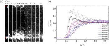
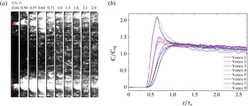
It should be noted that the applicability of the modelling of mass transport as a series of well-mixed reactors in Taylor–Couette vortex flow has been discussed recently and it was suggested that it is an insufficient representation of the actual process due to the observation of an ‘unmixed core’. Examples of the mass transfer results are shown in figures 3–6, for the flow states LTV, LWV, TWV and TTV, respectively. Expanded graphs of these experiments are shown in supplementary figures S2–S4. However, the ‘unmixed core’ is only observed here for the LWV flow state, as seen in figure 4 (
 $t/\unicode[STIX]{x1D70F}_{\unicode[STIX]{x1D708}}=0.57{-}0.71$
(40–50 s), where
 $\unicode[STIX]{x1D70F}_{\unicode[STIX]{x1D708}}=d^{2}/\unicode[STIX]{x1D708}$
) where the outline of the vortices can be seen with regions of lower Kalliroscope concentration at the centre. There is no obvious ‘unmixed core’ in the LTV flow state (figure 3) possibly due to the disruption of the flow state itself upon injection. With the addition of turbulence to the flow states, the ‘unmixed core’ is no longer observed, as seen in figures 5 and 6. Turbulence decreases local concentration gradients, so the loss of the ‘unmixed core’ is not surprising for these structures. Others have suggested a two-zone approach, where an inner core is separated from the outer part of the vortex, but recent publications spatially average concentrations over the whole vortex, even when the ‘unmixed core’ is present (Nemri et al.
Reference Nemri, Cazin, Charton and Climent2014, Reference Nemri, Charton and Climent2016).
Mass transfer results for the LWV structure (
 $Re=615$
,
 $v_{cylinder}=7.2~\text{cm}~\text{s}^{-1}$
,
 $\unicode[STIX]{x1D6FA}_{cylinder}=0.17~\text{Hz}$
) for a 20 psi (
 $3.1~\text{g}~\text{s}^{-1}$
,
 $0.32~\text{m}~\text{s}^{-1}$
) 50 g injection (2.7 % annulus,
 $t_{inject}=16~\text{s}$
). (a) Snapshots (0.75 cm wide) of the annulus between injection port rows 3 and 4 after injection illustrating the spatial concentration evolution. The numbers at the top of the panel represent the dimensionless time,
 $t/\unicode[STIX]{x1D70F}_{\unicode[STIX]{x1D708}}$
, of each image. The red arrows indicate the axial location of the injection port rows 3 and 4, which are 10 cm apart. (b) Temporal profile of the concentration in several vortices (solid lines) and the model (dashed lines) using the best fit intermixing coefficient. The
 $y$
-axis is normalized by the equilibrium concentration of Kalliroscope,
 $25~\text{g}~\text{l}^{-1}$
, and the
 $x$
-axis is dimensionless time, time divided by the momentum time scale (
 $\unicode[STIX]{x1D70F}_{\unicode[STIX]{x1D708}}=70.139~\text{s}$
). The black (vortex 1) and grey (vortex 8) lines correspond to the outermost vortices that are used as the input boundary conditions in the model regression. The model is regressed over the entire time profile (extending to
 $t/\unicode[STIX]{x1D70F}_{\unicode[STIX]{x1D708}}=8.6$
(600 s)), but only the shorter time response is shown here to better show the differences between vortex structures.

Injection mass transfer results for the TWV structure (
 $Re=2083$
,
 $v_{cylinder}=25~\text{cm}~\text{s}^{-1}$
,
 $\unicode[STIX]{x1D6FA}_{cylinder}=0.59~\text{Hz}$
) for a 20 psi (
 $3.1~\text{g}~\text{s}^{-1}$
,
 $0.32~\text{m}~\text{s}^{-1}$
) 50 g injection (2.7 % annulus,
 $t_{inject}=16~\text{s}$
). (a) Snapshots (0.75 cm wide) of the annulus between injection port rows 3 and 4 after injection illustrating the spatial concentration evolution. The numbers at the top of the panel represent the dimensionless time,
 $t/\unicode[STIX]{x1D70F}_{\unicode[STIX]{x1D708}}$
, of each image. The red arrows indicate the axial location of the injection port rows 3 and 4, which are 10 cm apart. (b) Temporal profile of the concentration in several vortices (solid lines) and the model (dashed lines) using the best fit intermixing coefficient. The
 $y$
-axis is normalized by the equilibrium concentration of Kalliroscope,
 $25~\text{g}~\text{l}^{-1}$
, and the
 $x$
-axis is dimensionless time, time divided by the momentum time scale (
 $\unicode[STIX]{x1D70F}_{\unicode[STIX]{x1D708}}=70.139~\text{s}$
). The black (vortex 1) and grey (vortex 8) lines correspond to the outermost vortices that are used as the input boundary conditions in the model regression. The model is regressed over the entire time profile (extending to
 $t/\unicode[STIX]{x1D70F}_{\unicode[STIX]{x1D708}}=8.6$
(600 s)), but only the shorter time response is shown here to better show the differences between vortex structures.

Mass transfer results for the TTV structure (
 $Re=10\,090$
,
 $v_{cylinder}=120~\text{cm}~\text{s}^{-1}$
,
 $\unicode[STIX]{x1D6FA}_{cylinder}=2.8~\text{Hz}$
) for a 20 psi (
 $3.1~\text{g}~\text{s}^{-1}$
,
 $0.32~\text{m}~\text{s}^{-1}$
) 50 g injection (2.7 % annulus,
 $t_{inject}=16~\text{s}$
). (a) Snapshots (0.75 cm wide) of the annulus between injection port rows 3 and 4 after injection illustrating the spatial concentration evolution. The numbers at the top of the panel represent the dimensionless time,
 $t/\unicode[STIX]{x1D70F}_{\unicode[STIX]{x1D708}}$
, of each image. The red arrows indicate the axial location of the injection port rows 3 and 4, which are 10 cm apart. (b) Temporal profile of the concentration in several vortices (solid lines) and the model (dashed lines) using the best fit intermixing coefficient. The
 $y$
-axis is normalized by the equilibrium concentration of Kalliroscope,
 $25~\text{g}~\text{l}^{-1}$
, and the
 $x$
-axis is dimensionless time, time divided by the momentum time scale (
 $\unicode[STIX]{x1D70F}_{\unicode[STIX]{x1D708}}=70.139~\text{s}$
). The black (vortex 1) and grey (vortex 9) lines correspond to the outermost vortices that are used as the input boundary conditions in the model regression. The model is regressed over the entire time profile (extending to
 $t/\unicode[STIX]{x1D70F}_{\unicode[STIX]{x1D708}}=8.6$
(600 s)), but only the shorter time response is shown here to better show the differences between vortex structures.

To maintain consistency with previous studies and between the turbulent and laminar wavy vortex flow states, the well-mixed model was applied to the LWV flow state, despite its drawbacks. However, the series of well-mixed reactors model is more applicable here, as there is only an axial concentration gradient present due to the azimuthal distribution of injection ports along the inner cylinder. Previous studies have all had single injection locations that injected a pulse of fluid, resulting in both an azimuthal and an axial concentration gradient. Even with the drawbacks of the model, the predictions match well with the experimentally measured vortex concentration profile. Additionally, this is the first study to introduce injection fluid non-intrusively (with flush mounted ports) and distributed throughout the annulus. In contrast to using a capillary inserted down through the annulus to inject fluid, here, the geometry of the annulus is undisturbed and the stability of the flow field to injection is known.
Overall, figures 3–6 show that as
 $Re$
increases, inter-vortex mass transfer also increases, shown both qualitatively in the
 $r$
–
 $z$
planes and quantitatively in the concentration profiles. As
 $Re$
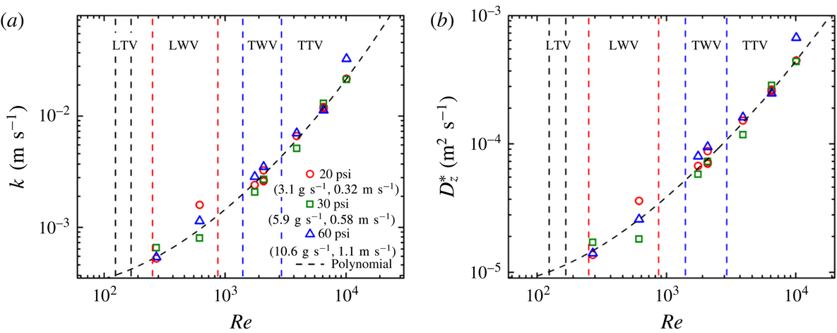
increases, the concentration profiles collapse to the final value at earlier times. Likewise, the axial space between injection port rows is illuminated with Kalliroscope faster in time. The dependence of the intermixing coefficient,
 $k$
, with
 $Re$
is shown in figure 7(a). The dashed line is a regressed, best fit quadratic equation,
 $k=9.97\times 10^{-11}Re^{2}+1.12\times 10^{-6}Re+2.32\times 10^{-4}$
, where
 $k$
has units of
 $\text{m}~\text{s}^{-1}$
. The intermixing coefficient can be linearly converted to an effective dispersion coefficient by the following equation:
 $D_{z}^{\ast }=2\unicode[STIX]{x1D706}k$
(Ohmura et al.
Reference Ohmura, Kataoka, Shibata and Makino1997) where
 $\unicode[STIX]{x1D706}$
is the axial wavelength and
 $D_{z}^{\ast }$
is the effective dispersion coefficient. The axial wavelength was determined by averaging all the vortex axial heights used during the intermixing coefficient regression. The trend of effective dispersion coefficient with
 $Re$
is shown in figure 7(b). The axial wavelengths for all of the vortex flow states tested here are very similar,
 ${\sim}$
1 cm, therefore
 $D_{z}^{\ast }$
has a similar trend to
 $k$
with a different magnitude. The dashed line in figure 7(b) is also a quadratic equation,
 $D_{z}^{\ast }=1.24\times 10^{-12}Re^{2}+3.11\times 10^{-8}Re+6.22\times 10^{-6}$
, where
 $D_{z}^{\ast }$
has units of
 $\text{m}^{2}~\text{s}^{-1}$
. A quadratic fit was chosen as it was the simplest fit that still maintained an
 $R^{2}>0.9$
. Traditionally, a power law fit is used for fitting mass transport data in TC flow for individual flow states. The best power law fit for the data here is
 $D_{z}^{\ast }=1.73\times 10^{-7}Re^{0.85}$
, which has
 $R^{2}=0.87$
. While the correlation coefficient is close to a polynomial fit, the trend of the data is not captured well, as seen in supplementary figure S5. The dispersion coefficient values determined here are similar to previous studies, which also report dispersion coefficients ranging from
 $10^{-5}$
to
 $10^{-4}~\text{cm}^{2}~\text{s}^{-1}$
despite using different TC cells and the use of Kalliroscope particles rather than fluorescent dyes. The dispersion coefficients are similar because of the insignificance of molecular diffusion in these flow structures. Molecular diffusion of the dyes is typically six orders of magnitude smaller than the regressed dispersion coefficients.
(a) Intermixing coefficient for all injection pressures and vortex flow states explored. All values have 50 g injections (2.7 % annulus,
 $4.7~\text{s}<t_{inject}<16~\text{s}$
). The black dashed line corresponds to the quadratic best fit, with an
 $R^{2}$
of 0.92. (b) Imaginary mass transfer coefficient for all injection pressures and vortex flow states explored. The effective dispersion coefficient trend is similar to the intermixing coefficient because the axial wavelengths for all vortices were
 ${\sim}$
1 cm. All values are from 50 g injections (2.7 % annulus,
 $4.7~\text{s}<t_{inject}<16~\text{s}$
). The black dashed line corresponds to the quadratic best fit, with an
 $R^{2}$
of 0.92. The vertical dashed lines in both (a) and (b) indicate the bounds of the various vortex structures.

The smoothly increasing mass transfer with increasing
 $Re$
across multiple vortex wave states was also seen by Nemri et al. (Reference Nemri, Climent, Charton, Lanoë and Ode2013, Reference Nemri, Charton and Climent2016). The main difference is in the large
 $Re$
regime, where they observe a plateau of dispersion coefficient in the TTV vortex state, whereas the work here does not observe any plateau, even at
 $Re\sim 10^{4}$
. This difference in high
 $Re$
behaviour is potentially due to the presence of the injection capillary inside the annulus in previous studies that altered the mass transfer in the TTV vortex state. Additionally, the quadratic fit is across the entire
 $Re$
range and is comparable to the plethora of different power law regressions for individual vortex states, which have power law exponents ranging from 0.8 to 2.8, as summarized by Nemri et al. (Reference Nemri, Charton and Climent2016).
Since figure 7(a,b) shows that there is no systematic effect of increasing drive pressure, a single value of the effective dispersion coefficient was used for all pressures at a given
 $Re$
for the analysis of vortex stability discussed in the following section. The mass transfer behaviour near the vortex stability boundaries was not explored here because of concerns about the vortex stability to radial injection. Near the critical
 $Re$
for transitions between vortices, the injection could locally or globally change the vortex state, altering the mass transport behaviour. Additionally, the work by Nemri et al. (Reference Nemri, Climent, Charton, Lanoë and Ode2013) shows a smoothly increasing trend of dispersion coefficient with
 $Re$
across multiple vortex states.
Previous studies have seen evidence that there is a difference in inter-vortex mass transfer at the inflow and outflow vortex boundaries. However, these studies used injection from a capillary that protrudes into the vortex through one boundary, but not the other. The asymmetry in the injection method may cause the asymmetry in the previous results. Moreover, mass transfer analysis is also typically only performed on two or three vortices. Here, 7–10 vortices are analysed with high speed (50 frames per second) measurement recording and intermixing coefficients are regressed simultaneously. From the data collected using this new TC cell design, there is no evidence of a difference in the intermixing coefficients at the inflow and outflow boundaries. Regression with two intermixing coefficients did not reduce the mean square error of the fit, nor did it change the appearance of the fit. Therefore, it appears that the apparent difference in inflow and outflow mass transfer is a result of specific injection geometries, rather than the vortex dynamics itself.
3.2 Vortex stability to injection
The mixing of two fluids is important to many different processes, often involving the mixing of large volumes of one fluid into another. TC cells have been shown to improve the performance of many mixing processes from bioreactors and chemical synthesis to photocatalysis. It is therefore important to know the limitations of each vortex type to fluid injection for the application of Taylor–Couette flows to mixing applications. Previous studies have focused on injections with a small amount mass of a tracer fluid when measuring mass transfer in Taylor–Couette cells reportedly not to disrupt the vortex structures with the injection. However, there is no evidence presented to quantify the extent of lack of disruption. Here, large volumes of fluid are injected to test the stability limits of each vortex type and a dimensionless number criterion is proposed to capture the governing stability behaviour and predict future process feasibility.
As before, four different vortex structures were examined (LTV, LWV, TWV and TTV) with turbulent/laminar pairs for each overall vortex type (Taylor and wavy vortex). The same
 $Re$
values were used for vortex stability measurements as were used for the mass transfer experiments, so that the experimentally measured effective dispersion coefficient could be used, except for the LTV, which used the predicted value from the regression of
 $D_{z}^{\ast }$
. For each experiment, the injection starts at
 $t/\unicode[STIX]{x1D70F}_{\unicode[STIX]{x1D708}}=0.43$
(30 s) after the start of recording and the behaviour of the vortex after the beginning of the injection is recorded for
 $t/\unicode[STIX]{x1D70F}_{\unicode[STIX]{x1D708}}=7.6$
(530 s). The Fourier transforms, both spatial and temporal, of each space–time plot were used to determine global vortex stability. The vortex was determined to be unstable to injection if the Fourier transform temporarily lost a dominant frequency during the injection. For all cases, after injection stops, the dominant frequencies eventually return as the initial vortex is the equilibrium state at the established
 $Re$
.
In these experiments exploring vortex stability, the fluid injected is identical to the fluid already in the annulus, removing any effects of changing fluid properties. Supplementary figure S6 and figure 8 show the behaviour of the LTV (
 $Re=146$
,
 $v_{cylinder}=1.7~\text{cm}~\text{s}^{-1}$
) to the slowest, smallest (20 psi (
 $3.1~\text{g}~\text{s}^{-1}$
,
 $0.32~\text{m}~\text{s}^{-1}$
), 20 g (1.1 % annulus,
 $t_{inject}=6.4~\text{s}$
)) and fastest, largest (60 psi (
 $10.6~\text{g}~\text{s}^{-1}$
 $1.1~\text{m}~\text{s}^{-1}$
), 100 g (5.5 % annulus,
 $t_{inject}=9.5~\text{s}$
)) injection, respectively. The LTV is the least stable vortex structure tested here, which is expected as it is also at the lowest
 $Re$
tested. While globally stable at the slowest and smallest injection (20 psi (
 $3.1~\text{g}~\text{s}^{-1}$
,
 $0.32~\text{m}~\text{s}^{-1}$
), 20 g (1.1 % annulus,
 $t_{inject}=6.4~\text{s}$
)), there are perturbations present that persist over the course of the whole experiment. The perturbations, seen in supplementary figure S6, are most likely due to the upward axial flow from the injection, as the perturbations are only present in the upper portion of the annulus and become progressively more pronounced at each higher injection port row. There is a vertical axial flow during injection because the only fluid outlet from the annulus is through the top cap. The vertical axial flow triggers an oscillation in the LTV in the upper portion of the annulus that is never fully recovered from within the time scales measured here. There is no apparent frequency of this oscillation as the pattern is different between each injection port row.
Space–time and corresponding Fourier transform plots for LTV (
 $Re=146$
,
 $v_{cylinder}=1.7~\text{cm}~\text{s}^{-1}$
,
 $\unicode[STIX]{x1D6FA}_{cylinder}=0.041~\text{Hz}$
) 60 psi (
 $10.6~\text{g}~\text{s}^{-1}$
,
 $1.1~\text{m}~\text{s}^{-1}$
) 100 g (5.5 % annulus,
 $t_{inject}=9.5~\text{s}$
), showing unstable behaviour. The depicted view is of the entire annulus height. The axial locations of the injection port rows are
 $z/d=10$
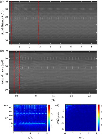
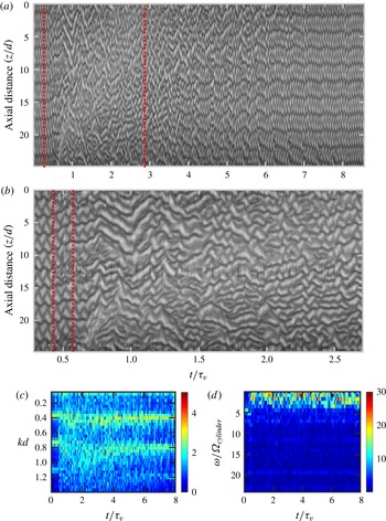
, 21, 33 and 45 (8, 18, 28 and 38 cm). The periodic grey spots are the injection port covers. In the top row, all ports are visible, and in the second row, every other port is visible. (a) Space–time plot showing the entire time response of the vortex structure as a function of dimensionless time. The vertical red dashed lines show the time range that panel (b) shows. (b) Space–time plot showing the short time response of the vortex during and after injection as a function of dimensionless time. The vertical red dashed lines enclose the injection duration. (c) Spatial Fourier transform contour for the entire time domain. The colour represents the log of the magnitude of the complex modulus of the Fourier transform. (d) Temporal Fourier transform contour for the entire time domain.

Vortex instability can be seen in figure 8, which shows the highest injection speed and amount (60 psi (
 $10.6~\text{g}~\text{s}^{-1}$
 $1.1~\text{m}~\text{s}^{-1}$
), 100 g (5.5 % annulus,
 $t_{inject}=9.5~\text{s}$
)). At this injection condition, the vortex structure is temporarily lost during injection, as denoted by the loss of the wavenumber (spatial frequency) at
 $kd\sim 1$
(
 $k\sim 1.2~\text{cm}^{-1}$
). The LTV’s instability to axial flow is also apparent in figure 8, as the vortex structure is substantially more disrupted at the top than it is at the bottom of the annulus. When the LTV does recover, the wavenumber (spatial frequency) is lower, indicative of wider vortices. This decrease of wavenumber (spatial frequency) was also observed during initial characterization of this device with the TTV structure (Wilkinson & Dutcher Reference Wilkinson and Dutcher2017), and is due to a loss of one or more vortices out of the top of the annulus. The vortices move upward with the axial flow and leave the annulus and are not reformed. The loss of these vortices causes an axial expansion of the remaining vortices to fill the annulus height.
Figures 9 and 10 show the behaviour of the lower
 $Re$
value of the LWV structure (
 $Re=270$
,
 $v_{cylinder}=3.2~\text{cm}~\text{s}^{-1}$
,
 $\unicode[STIX]{x1D6FA}_{cylinder}=0.076~\text{Hz}$
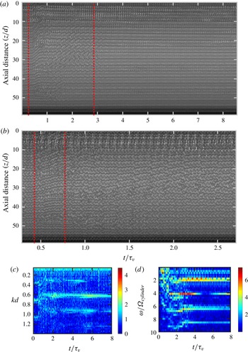
) at the two extremes of the injection conditions. Figure 9 shows stable behaviour at 20 psi (
 $3.1~\text{g}~\text{s}^{-1}$
,
 $0.32~\text{m}~\text{s}^{-1}$
), 20 g (1.1 % annulus,
 $t_{inject}=6.4~\text{s}$
). The injection does cause a small local perturbation in the wave structure that recovers after
 ${\sim}t/\unicode[STIX]{x1D70F}_{\unicode[STIX]{x1D708}}=2.1$
(
 ${\sim}150~\text{s}$
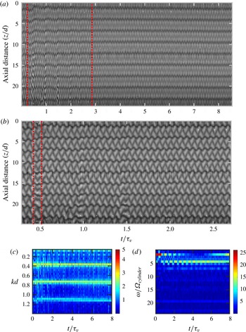
). Figure 10 illustrates the interesting unstable behaviour of the LWV, where the high injection mass and speed (60 psi (
 $10.6~\text{g}~\text{s}^{-1}$
,
 $1.1~\text{m}~\text{s}^{-1}$
), 100 g (5.5 % annulus,
 $t_{inject}=9.5~\text{s}$
)) overwhelm the vortex structure. The space–time plots show a prolonged period of chaotic structure, corresponding to the change in both the temporal and spatial Fourier spectra. Interestingly, at
 $t/\unicode[STIX]{x1D70F}_{\unicode[STIX]{x1D708}}=0.71$
(
 ${\sim}50~\text{s}$
), there is simultaneously both upward and downward vertical motions of the remaining vortices in figure 10. While the LWV does eventually fully reform, there is an increase in the wavenumber (spatial frequency) as there are more vortices after injection than before injection. Additionally, even at
 $t/\unicode[STIX]{x1D70F}_{\unicode[STIX]{x1D708}}=7.6$
(530 s) from injection, the LWV has not completely recovered, as demonstrated by the perturbations in the wave structure.
Space–time and corresponding Fourier transform plots for LWV (
 $Re=270$
,
 $v_{cylinder}=3.2~\text{cm}~\text{s}^{-1}$
,
 $\unicode[STIX]{x1D6FA}_{cylinder}=0.076~\text{Hz}$
) 20 psi (
 $3.1~\text{g}~\text{s}^{-1}$
,
 $0.32~\text{m}~\text{s}^{-1}$
) 20 g (1.1 % annulus,
 $t_{inject}=6.4~\text{s}$
), showing stable behaviour. The depicted view is between injection port rows 2–4. The axial locations of the injection port rows are
 $z/d=1.2$
, 13 and 25 (1, 11 and 21 cm). (a) Space–time plot showing the entire time response of the vortex structure as a function of dimensionless time. The vertical red dashed lines show the time range that panel (b) shows. (b) Space–time plot showing the short time response of the vortex during and after injection as a function of dimensionless time. The vertical red dashed lines enclose the injection duration. (c) Spatial Fourier transform contour for the entire time domain. (d) Temporal Fourier transform contour for the entire time domain. The colour represents the log of the magnitude of the complex modulus of the FFT.

Space–time and corresponding Fourier transform plots for LWV (
 $Re=270$
,
 $v_{cylinder}=3.2~\text{cm}~\text{s}^{-1}$
,
 $\unicode[STIX]{x1D6FA}_{cylinder}=0.076~\text{Hz}$
) 60 psi (
 $10.6~\text{g}~\text{s}^{-1}$
,
 $1.1~\text{m}~\text{s}^{-1}$
) 100 g (5.5 % annulus,
 $t_{inject}=9.5~\text{s}$
), showing unstable behaviour. The depicted view is between injection port rows 2–4. The axial locations of the injection port rows are
 $z/d=1.2$
, 13 and 25 (1, 11 and 21 cm). (a) Space–time plot showing the entire time response of the vortex structure as a function of dimensionless time. The vertical red dashed lines show the time range that panel (b) shows. (b) Space–time plot showing the short time response of the vortex during and after injection as a function of dimensionless time. The vertical red dashed lines enclose the injection duration. (c) Spatial Fourier transform contour for the entire time domain. (d) Temporal Fourier transform contour for the entire time domain. The colour represents the log of the magnitude of the complex modulus of the FFT.

Supplementary figures S7, S8 and figure 11 show the behaviour of the same LWV structure but at a higher
 $Re$
(
 $Re=615$
,
 $v_{cylinder}=7.2~\text{cm}~\text{s}^{-1}$
,
 $\unicode[STIX]{x1D6FA}_{cylinder}=0.17~\text{Hz}$
). Supplementary figure S7 shows the stable response of the vortex at 20 g (1.1 % annulus,
 $t_{inject}=3.4~\text{s}$
) and 30 psi (
 $5.9~\text{g}~\text{s}^{-1}$
,
 $0.58~\text{m}~\text{s}^{-1}$
). Despite the higher drive pressure than that used in figure 9, the LWV shows fewer effects due to injection. Supplementary figure S8 and figure 11 show two different unstable responses of the high
 $Re$
LWV at
 $Re=615$
,
 $v_{cylinder}=7.2~\text{cm}~\text{s}^{-1}$
,
 $\unicode[STIX]{x1D6FA}_{cylinder}=0.17~\text{Hz}$
. Supplementary figure S8 shows the response to a 60 psi (
 $10.6~\text{g}~\text{s}^{-1}$
,
 $1.1~\text{m}~\text{s}^{-1}$
), 100 g (5.5 % annulus,
 $t_{inject}=9.5~\text{s}$
) injection. Figure 11 shows the response to a 60 psi (
 $10.6~\text{g}~\text{s}^{-1}$
,
 $1.1~\text{m}~\text{s}^{-1}$
), 240 g (13 % annulus,
 $t_{inject}=22~\text{s}$
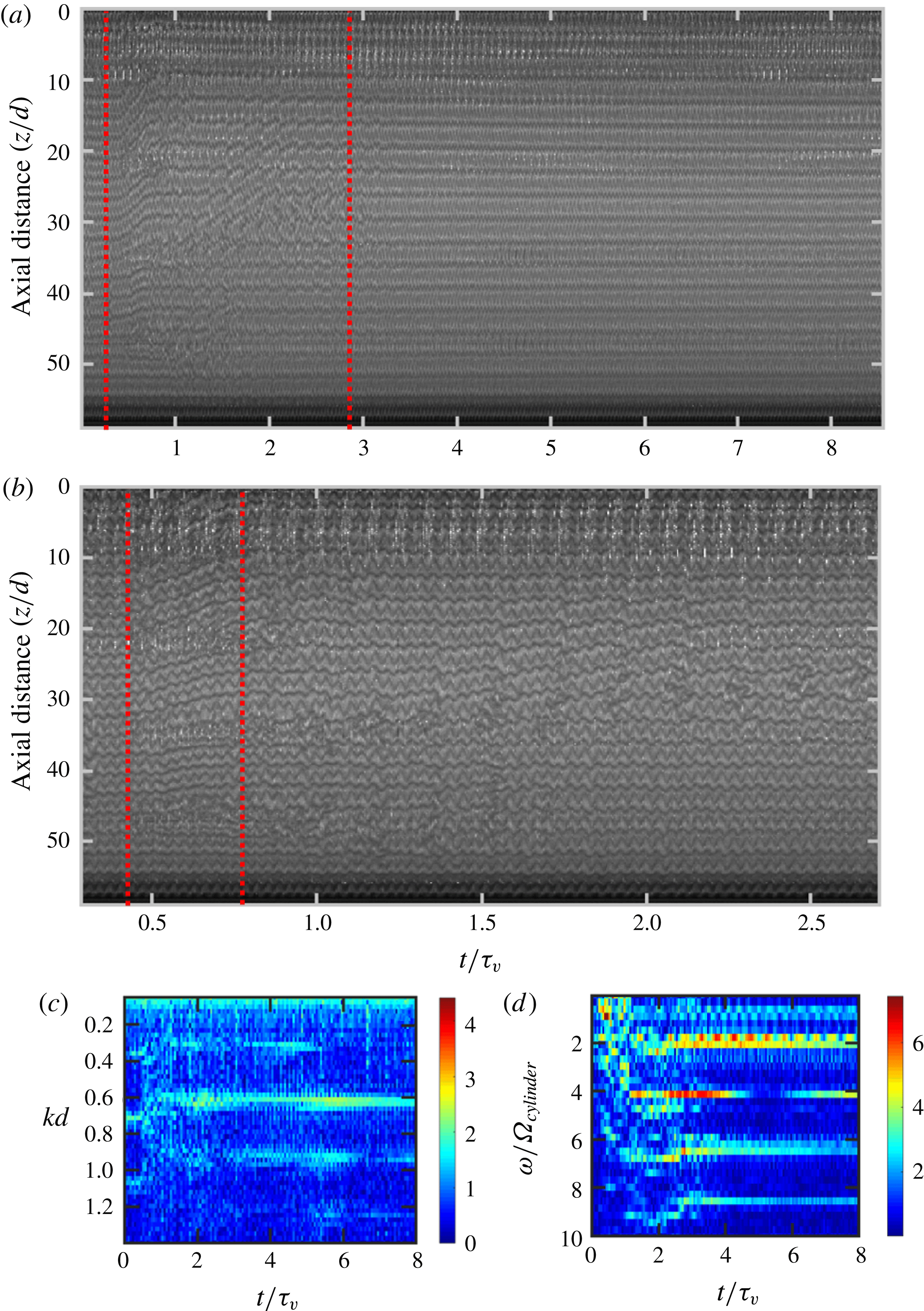
) injection. There is a loss of two vortex pairs out of the top of the annulus, causing the decrease in wavenumber (spatial frequency) and a perturbation in the wave structure that persists for
 $t/\unicode[STIX]{x1D70F}_{\unicode[STIX]{x1D708}}=3.1$
(
 ${\sim}$
220 s) after the start of injection. The recovery time of the LWV is less at a higher
 $Re$
, as seen in figure 11, compared to the recovery time at lower
 $Re$
, as seen in figure 10. The reduced effect of injection as
 $Re$
increases indicates that the increased effective dispersion coefficient stabilizes the vortex to injection as it is now better able to transport the injected mass through the vortex structure.
Space–time and corresponding Fourier transform plots for LWV (
 $Re=615$
,
 $v_{cylinder}=7.2~\text{cm}~\text{s}^{-1}$
,
 $\unicode[STIX]{x1D6FA}_{cylinder}=0.17~\text{Hz}$
) 60 psi (
 $10.6~\text{g}~\text{s}^{-1}$
,
 $1.1~\text{m}~\text{s}^{-1}$
) 240 g (13 % annulus,
 $t_{inject}=22~\text{s}$
), showing unstable behaviour. The depicted view is the entire annulus. The axial locations of the injection port rows are
 $z/d=12$
, 24, 36 and 48 (10, 20, 30 and 40 cm). (a) Space–time plot showing the entire time response of the vortex structure as a function of dimensionless time. The vertical red dashed lines show the time range that panel (b) shows. (b) Space–time plot showing the short time response of the vortex during and after injection as a function of dimensionless time. The vertical red dashed lines enclose the injection duration. (c) Spatial Fourier transform contour for the entire time domain as a function of dimensionless time. (d) Temporal Fourier transform contour for the entire time domain as a function of dimensionless time. The colour represents the log of the magnitude of the complex modulus of the FFT.
Overall, as
 $Re$
increases the vortices become more stable to injection mass and pressure, both within the same vortex structure type (e.g. low versus high
 $Re$
LWV) and between vortex structures (e.g. TWV and TTV). Vortex stability is dependent on both injection mass and pressure, as vortices can be stable to 100 g (5.5 % annulus,
 $t_{inject}=32~\text{s}$
) injections at 20 psi (
 $3.1~\text{g}~\text{s}^{-1}$
,
 $0.32~\text{m}~\text{s}^{-1}$
) but not at 60 psi (
 $10.6~\text{g}~\text{s}^{-1}$
,
 $1.1~\text{m}~\text{s}^{-1}$
) and likewise stable to 60 psi (
 $10.6~\text{g}~\text{s}^{-1}$
,
 $1.1~\text{m}~\text{s}^{-1}$
) at 50 g (2.7 % annulus,
 $t_{inject}=4.7~\text{s}$
) injection but not at 100 g (5.5 % annulus,
 $t_{inject}=9.5~\text{s}$
) injection. Therefore, both injection mass and pressure act to destabilize the vortices. Injection mass and pressure increase the amount of mass introduced into the vortex at the injection port location, which can only be ultimately removed from the top edge of the annulus. The injected mass then must be transferred between vortices, all the vortices must move upward, or a combination of the two. The inter-vortex mass transfer, therefore, acts to stabilize the vortices.
The time scale associated with the destabilizing injection can be described as
 $$\begin{eqnarray}\displaystyle \unicode[STIX]{x1D70F}_{inject}(\text{s})=S/t_{inject}v_{inject}^{2}, & & \displaystyle\end{eqnarray}$$
where
 $S$
is the interfacial area between vortices
 $[\unicode[STIX]{x03C0}(r_{o}^{2}-r_{i}^{2})]$
. This interfacial area was chosen as it is the area that the mass injected must cross to be transported to the exit of the annulus. The injection time (
 $t_{inject}$
) and average linear velocity of the injected fluid (
 $v_{inject}$
), are found from
 $$\begin{eqnarray}\displaystyle v_{inject}~(\text{m}~\text{s}^{-1})=\frac{\text{Injection}\;\text{rate}~(\text{g}~\text{s}^{-1})}{\unicode[STIX]{x1D70C}(\text{g}~\text{m}^{-3})~\text{Injection}\;\text{area}~(\text{m}^{2})} & & \displaystyle\end{eqnarray}$$
and
 $$\begin{eqnarray}\displaystyle t_{inject}\;(\text{s})=\frac{\text{Injection}\;\text{mass}\;(\text{g})}{\text{Injection}\;\text{rate}~(\text{g}~\text{s}^{-1})}. & & \displaystyle\end{eqnarray}$$
Injection rate in (3.2) and (3.3) is a function of injection pressure as defined in the calibration in figure 1,
 $\unicode[STIX]{x1D70C}$
is the density of the injected fluid, injection area is the cross-sectional area of the injection ports
 $(9.677\times 10^{-6}~(\text{m}^{2}))$
. The value of
 $v_{inject}$
varies from
 $0.32~\text{m}~\text{s}^{-1}$
at 20 psi injections to
 $1.1~\text{m}~\text{s}^{-1}$
at 60 psi injections. The time scale of injection from (3.1) captures the extent of the perturbation induced by the injection. As
 $\unicode[STIX]{x1D70F}_{inject}$
decreases, the effect of the injection conditions increases.
Similarly, a stabilizing time scale associated with mass transport can be constructed from the effective dispersion coefficient. Since
 $D_{z}^{\ast }$
is regressed from the mass transport across the vortex interfacial area,
 $S$
is used in the mass transport time scale as well, resulting in the following equation:
 $$\begin{eqnarray}\displaystyle \unicode[STIX]{x1D70F}_{transport}\;(\text{s})=S/D_{z}^{\ast }. & & \displaystyle\end{eqnarray}$$
As the time scale of mass transport increases, the ability of the vortex structure to transport mass axially decreases.
A non-dimensional number can then be constructed by taking the ratio of these two time scales. Taking the ratio of the time scale of mass transport to injection results in the destabilizing drivers in the numerator (
 $t_{inject}$
and
 $v_{inject}$
) and the stabilizing driver in the denominator (
 $D_{z}^{\ast }$
), creating the following dimensionless number:
 $$\begin{eqnarray}\displaystyle \text{Stability number}=\unicode[STIX]{x1D70F}_{transport}/\unicode[STIX]{x1D70F}_{inject}=t_{inject}v_{inject}^{2}/D_{z}^{\ast }. & & \displaystyle\end{eqnarray}$$
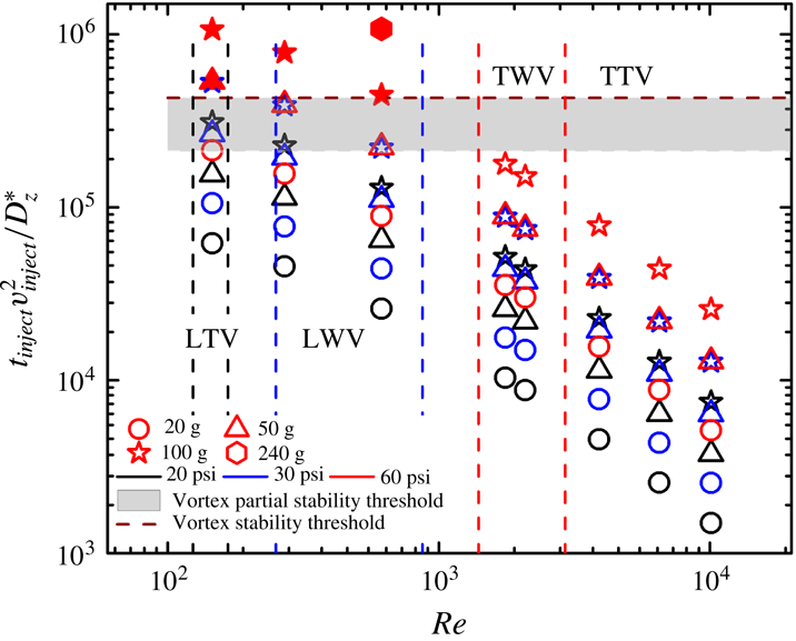
High stability numbers correspond to scenarios where it takes longer for mass to be transported through the vortex structure than the time scale of injection, resulting in unstable conditions. Figure 12 shows how the stability number varies for each experimental condition explored here. The open symbols are stable conditions and the closed symbols are unstable conditions. At stability number values above
 $4.3\times 10^{5}$
, all vortices become unstable.
Dimensionless stability criterion values for all the experimental conditions explored. The colour of the symbol corresponds to injection pressure (black
 $=$
20 psi (
 $3.1~\text{g}~\text{s}^{-1}$
,
 $0.32~\text{m}~\text{s}^{-1}$
), blue
 $=$
30 psi (
 $5.9~\text{g}~\text{s}^{-1}$
,
 $0.58~\text{m}~\text{s}^{-1}$
) and red
 $=$
60 psi (
 $10.6~\text{g}~\text{s}^{-1}$
,
 $1.1~\text{m}~\text{s}^{-1}$
)), the shape corresponds to the injection mass (circle
 $=$
20 g (1.1 % annulus), triangle
 $=$
50 g (2.7 % annulus), star
 $=$
100 g (5.5 % annulus) and hexagon
 $=$
240 g (13 % annulus)) and the fill corresponds to the stability of the flow state (open
 $=$
stable and filled
 $=$
unstable). The maroon horizontal dashed line corresponds to the global stability threshold, such that stability number values above that threshold correspond to unstable behaviour. The grey region corresponds to a partial stability threshold where only a portion of the vortex structure is unstable or exhibits perturbations and/or wave splitting/joining behaviour that does not compromise the stability of the entire structure occurs.

There is a region of partial stability beneath this instability threshold where vortices are stable overall, but exhibit perturbations and/or wave splitting/joining behaviour that does not compromise the stability of the entire structure, similar to what has been observed previously (Coles Reference Coles1965). This region is comprised of the shaded grey region in figure 12, and the lower limit of the region is when the stability number is
 $2.1\times 10^{5}$
. To the authors’ knowledge, this is the first stability criterion developed for mixing in TC flow. This criterion can be used to identify which vortex is required for a given mixing process condition. It can also be used to identify what injection conditions can be used if a specific vortex structure is required.
It should be noted that the stability number has only been tested for this annulus gap width and radius ratio. This limitation excludes testing the stability number’s invariance to
 $S$
and radius ratio, as presented here. The injection time scale could be scaled with the injection area, rather than
 $S$
to recapture a dependence of stability with
 $S$
. The annulus gap width, along with radius ratio, confines the injection radially. If the injection is strong enough for the stream exiting the injection port to reach the outer wall, the additional flow patterns generated will likely further destabilize the vortex structure. A possible scaling of this mode of instability could be
 $v_{inject}/v_{vortex}$
or could be found by comparing the kinetic energy of the injection stream to the vortex, but further exploration is required. The annulus gap width is captured in
 $Re$
, which controls the effective dispersion coefficient, but no exploration of the effect of annulus gap width is explored here to confirm if this dependence is sufficient. Additionally, this work does not explore injection of fluids of significantly different properties from the fluid already in the annulus, namely fluids of different densities or viscosities. Injection of a fluid of differing properties would then create a scenario where the solution properties between vortices, and even spatially within a vortex, vary as mass is transferred within and between vortices. The spatial and temporal gradient in solution properties can potentially locally change vortex behaviour, increasing analysis complexity. Finally, only inner cylinder rotation is explored in the present study. With the addition of independent rotation of the outer cylinder, it is possible to have two separate wave states that exist at the same total
 $Re$
. Measuring the mass transfer of two different vortices with the same total
 $Re$
would elucidate the relative importance of the vortex structure to
 $Re$
.
4 Conclusions
Taylor–Couette flows have many applications in chemical reactions, materials synthesis, water treatment and solution processing, all of which involve mixing solutions together in a controlled manner to improve process performance. Using a modified Taylor–Couette cell design that non-intrusively incorporates injection ports into the inner cylinder, vortex stability to radial fluid injection was explored as a function of
 $Re$
encompassing four different wave states, with and without turbulence, and across two orders of magnitude of
 $Re$
. The injection design minimizes azimuthal concentration gradients, resulting in simplified mass transfer analysis. Inter-vortex mass transfer was measured for each vortex structure and
 $Re$
explored by injecting a Kalliroscope solution into distilled water and tracking the concentration of Kalliroscope within each vortex. An inter-vortex mixing model is used to calculate an intermixing coefficient, which is then converted into an effective dispersion coefficient. A quadratic relationship between the effective dispersion coefficient and
 $Re$
was developed from the data.
This study is also the first to explore vortex stability to injection and intentionally destabilize vortex structures. A non-dimensional stability number was created to predict whether a vortex will be stable to injection or unstable. This stability number is proportional to the time of injection, the square of injection speed and inversely proportional to the effective dispersion coefficient. In addition to yielding a global stability criterion, a partial stability region also emerged, where the overall vortex structure is stable, but perturbation and/or wave splitting/joining can occur without compromising the entire vortex structure. The stability number can inform accessible injection conditions for a desired process; for a given amount of fluid intended to be mixed, a corresponding maximum injection speed can be determined for the desired
 $Re$
of operation.
Acknowledgements
We like to thank M. Jensen, R. Jones, R. Bystrum and P. Ness for their work in manufacturing the TC cell. This work was supported primarily by the National Science Foundation through the University of Minnesota MRSEC under award no. DMR-1420013. This research was conducted with Government support under and awarded by Department of Defense, Air Force Office of Scientific Research, National Defense Science and Engineering Graduate (NDSEG) Fellowship, 32 CFR 168a.
Supplementary materials
Supplementary materials are available at https://doi.org/10.1017/jfm.2018.596.