1 Introduction
Since the groundwork laid by Taylor & Saffman (Reference Taylor and Saffman1959), our understanding of travelling menisci in confined environments has been increasingly refined. As the non-wetting disperse phase advances, a lubrication film of external phase develops between the interface and the substrate, where dissipation is localized. Droplet motion depends on the shape of that interface, as well as its physicochemical properties. This was first evidenced by Bretherton (Reference Bretherton1961), in the case of a slender bubble travelling in a horizontal capillary tube. The thickness of the lubrication film was found to be set by a balance between capillary and viscous forces in the external phase, expressed via the capillary number,
 $Ca=\unicode[STIX]{x1D702}_{o}U_{d}/\unicode[STIX]{x1D6FE}$
, where
 $\unicode[STIX]{x1D702}_{o}$
,
 $U_{d}$
and
 $\unicode[STIX]{x1D6FE}$
are, respectively, the external phase viscosity, the bubble velocity and the interfacial tension. For
 $Ca\leqslant 10^{-3}$
, and assuming a vanishing tangential stress at the interface (stress-free boundary condition), this classical analysis predicts a film thickness scaling in
 $Ca^{2/3}$
far from the front meniscus, and an oscillation of the interface at the back of the bubble. This theory was then extended to different model boundary conditions: incompressible interfaces (the
 $Ca^{2/3}$
scaling was recovered with corrections to the prefactors by Shen et al. (Reference Shen, Gleason, McKinley and Stone2002) and Cantat (Reference Cantat2013)) and viscous droplets (Hodges, Jensen & Rallison (Reference Hodges, Jensen and Rallison2004) found an additional contribution scaling in
 $Ca$
). That approach was also adapted to non-axisymmetric problems, such as two-phase displacement through Hele-Shaw cells. In such a configuration, Park & Homsy (Reference Park and Homsy1984) extended Bretherton’s results to a meniscus of arbitrary shape with an asymptotic approach. Similarly, the shape of the lubrication film for a bubble of radius much larger than the cell gap was derived for a stress-free boundary condition by Burgess & Foster (Reference Burgess and Foster1990). The shape of the lubrication film was also studied by Halpern & Secomb (Reference Halpern and Secomb1992) in the framework of the derivation of the speed of red blood cells squeezed between two parallel plates. In that later case, the interface is rigid instead of being stress-free.
These theoretical results were found to be in good agreement with experimental work ever since Bretherton’s (Reference Bretherton1961) early work, sometimes with discrepancies attributed to additional effects neglected in the model. Recent examples include surfactant-covered bubbles (Denkov et al. Reference Denkov, Tcholakova, Golemanov, Subramanian and Lips2006) and viscous droplets (Huerre et al. Reference Huerre, Theodoly, Leshansky, Valignat, Cantat and Jullien2015). However, most of these works could only access average quantities over the size of the droplet, since the height of the lubrication film was generally deduced from the velocities of the droplet and external phase, via the conservation of the flow. Interferometry methods were used to measure the height of thin films directly, but only for non-confined cases such as a soap film (Mysels & Cox Reference Mysels and Cox1962), the wetting film left on a plate (Snoeijer et al. Reference Snoeijer, Ziegler, Andreotti, Fermigier and Eggers2008) or the lubrication film under a foam (Denkov et al. Reference Denkov, Tcholakova, Golemanov, Subramanian and Lips2006). In this context, a previous study investigating droplets confined in a microfluidic Hele-Shaw cell via reflection interference contrast microscopy (RICM) provided the first direct measurement of the lubrication film thickness in a confined geometry (Huerre et al. Reference Huerre, Jullien, Theodoly and Valignat2016). Though it was not the focus of that article, the lubrication film was found to exhibit a complex three-dimensional (3D) topography, which had been predicted by Burgess & Foster (Reference Burgess and Foster1990) but never quantitatively characterized experimentally. This challenging experimental characterization is the aim of the present article.
Fluorinated-oil droplets travel through a microfluidic Hele-Shaw cell, in an aqueous solution containing a single surfactant (decyltrimethylammonium bromide,
 $\text{C}_{10}$
TAB). They are confined into a pancake shape, as the cell gap is much smaller than the droplet diameter. Using RICM, we measure lubrication film thicknesses down to a precision of a few nanometres (Huerre et al.
Reference Huerre, Jullien, Theodoly and Valignat2016). We find the lubrication films to exhibit a complex 3D shape: ravines develop along the sides, while a bump appears at the rear of the droplet.
The parameters governing this out-of-equilibrium shape are outside of the range accessible to current direct numerical simulations (Zhu & Gallaire Reference Zhu and Gallaire2016). Especially, the capillary number is too low, and the aspect ratio between the film thickness and the droplet size is too large. It is thus crucial to develop approximate analytical models to understand and predict the observed shapes. To this aim we develop a model based on the lubrication approximations at various levels of refinement. The film profile along the symmetry plane of the drop is described using a two-dimensional (2D) geometry in § 4. An important result of the paper is that the stress-free condition at the liquid–liquid interface applies at the front of the droplet, whereas Marangoni effects are important at the rear. We show that surfactant accumulation at the droplet rear induces an interface stiffening, which leads to a film thickening that may reach a factor 2, as predicted by Park (Reference Park1992). The surfactant transport is shown to be dominated by convection in this region, and the lubrication equations coupled to the surfactant transport are solved in this regime, leading to good agreement with experiment. In contrast, in § 5, a full 3D model is used to describe the ravines on the sides, at the price of the simplified stress-free condition at the liquid–liquid interface, following Burgess & Foster (Reference Burgess and Foster1990).
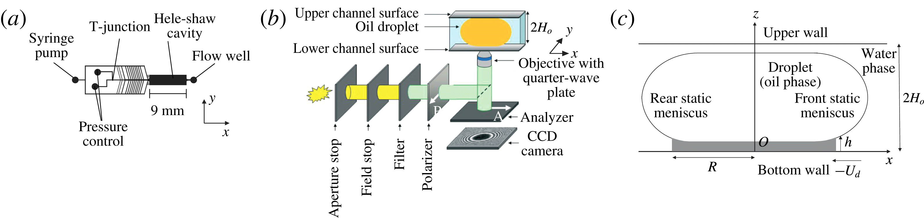
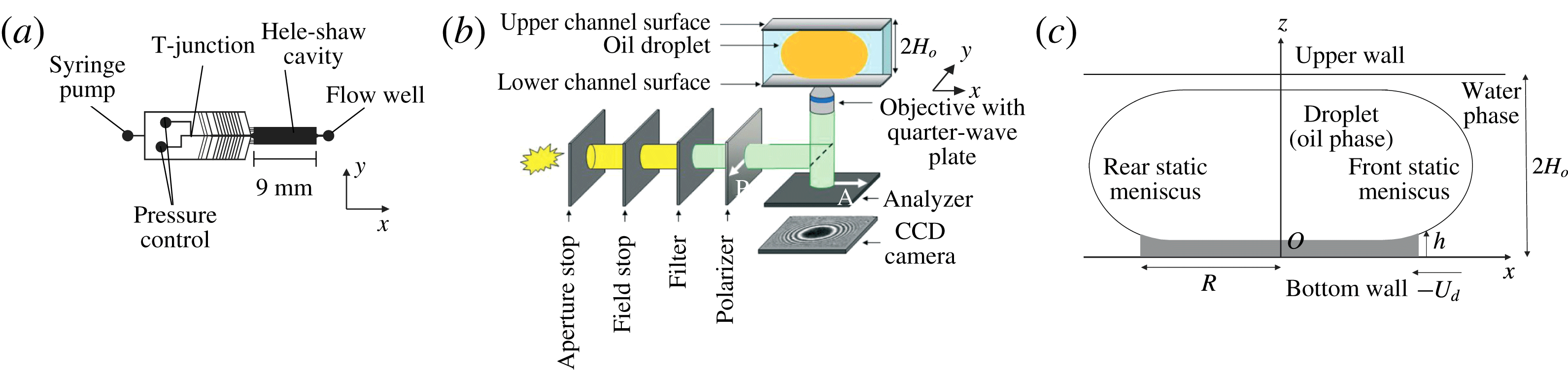
Schematic representation of the experimental set-up. (a) Top view of the microfluidic chip. (b) Optical set-up used for reflection interference contrast microscopy (RICM). The Hele-Shaw cell is placed just above the objective so that the thin film of water between the bottom wall and the oil droplet is imaged. (c) Side view of the droplet in its frame of reference. The grey domain is the region of the film that can be characterized.
2 Experimental set-up
2.1 Materials and methods
Fluorinated-oil droplets (C
 $_{6}$
F
 $_{14}$
: 3M Fluorinert FC-72, of viscosity
 $\unicode[STIX]{x1D702}_{i}=0.64~\text{mPa}~\text{s}$
) are travelling in an aqueous solution of C
 $_{10}$
TAB (Sigma-Aldrich, concentration
 $c_{o}=990~\text{mM}$
) and NaCl (concentration
 $c_{salt}=1~\text{M}$
). The high concentration of salt ensures that the Debye length is decreased down to
 $\unicode[STIX]{x1D706}_{d}=0.2~\text{nm}$
, i.e. much smaller than the typical thickness of the lubrication films in our experiment. The viscosity of the external phase was measured to be
 $\unicode[STIX]{x1D702}_{o}=2.5~\text{mPa}~\text{s}$
(Anton Paar MCR 302 rheometer), while the interfacial tension between the two phases was measured to be
 $\unicode[STIX]{x1D6FE}=15~\text{mN}~\text{m}^{-1}$
(KRUSS DSA30 tensiometer).
The microfluidic chip is shown in figure 1(a). The upper part of the chamber is made of polydimethylsiloxane (PDMS) and fabricated using soft photolithography (Xia & Whitesides Reference Xia and Whitesides1998). It is permanently bonded to a glass slide via oxygen plasma. The PDMS layer is covered by a second glass slide, to ensure that the channel does not deform even at the highest pressures applied (Taccoen Reference Taccoen2015). The droplets are generated at a T-junction using a MAESFLO pressure controller, and accelerated with a Nemesys syringe pump. The droplets then reach a Hele-Shaw cell of height
 $2H_{o}=14~\unicode[STIX]{x03BC}\text{m}$
, width
 $l_{o}=2500~\unicode[STIX]{x03BC}\text{m}$
and length
 $L_{o}=9~\text{mm}$
. The external phase flow is controlled by the syringe pump and ranges from 9 to
 $36~\unicode[STIX]{x03BC}\text{L}~\text{min}^{-1}$
. The resulting droplet velocities
 $U_{d}$
in the Hele-Shaw cavity range from 2300 to
 $14\,700~\unicode[STIX]{x03BC}\text{m}~\text{s}^{-1}$
, which correspond to capillary numbers between
 $3.9\times 10^{-4}$
and
 $2.4\times 10^{-3}$
. The flow is measured at the exit of the channel with a Fluigent flow well.
The droplets are large enough to adopt a pancake shape of height very close to
 $2H_{o}$
and radius much larger than
 $H_{o}$
in the Hele-Shaw cell (see figure 1
c). The droplet is separated from the top and bottom cell walls by a continuous thin film of external phase, stabilized by surfactant and hydrodynamical forces. Outside this region, the interface is almost not deformed by the flow and keeps its equilibrium shape. For this reason, the domain of continuous phase trapped between the lateral part of the interface and the bottom (respectively, top) wall is referred to as the bottom (respectively, top) static meniscus (see figure 1
c). All the experiments have been performed with a thin-film radius of
 $R\simeq 91\pm 6~\unicode[STIX]{x03BC}\text{m}$
.
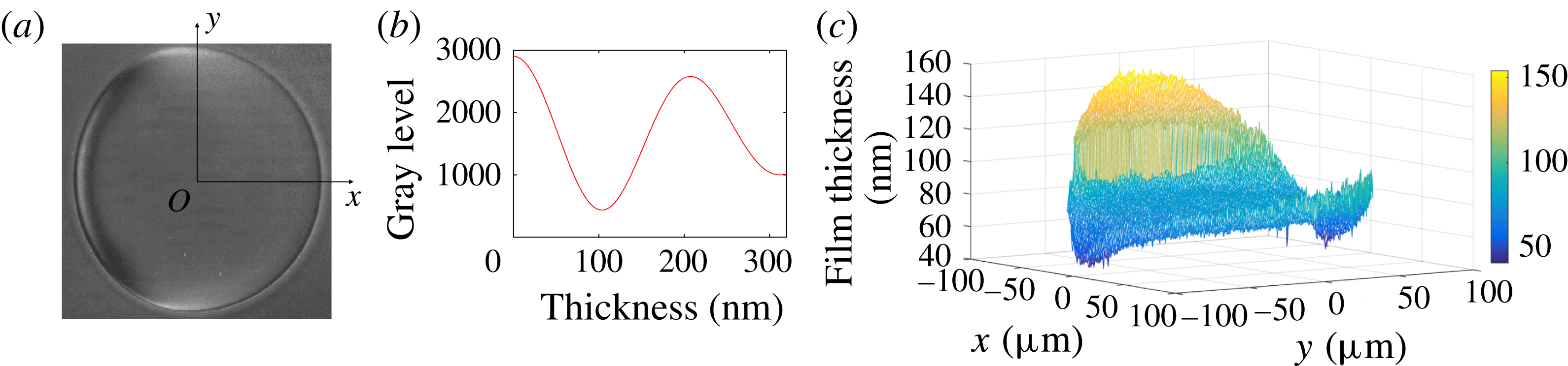
(a) RICM picture of a droplet travelling through the Hele-Shaw cell, in the
 $x$
direction. The droplet diameter is
 $170~\unicode[STIX]{x03BC}\text{m}$
in this image;
 $Ca=7.2\times 10^{-4}$
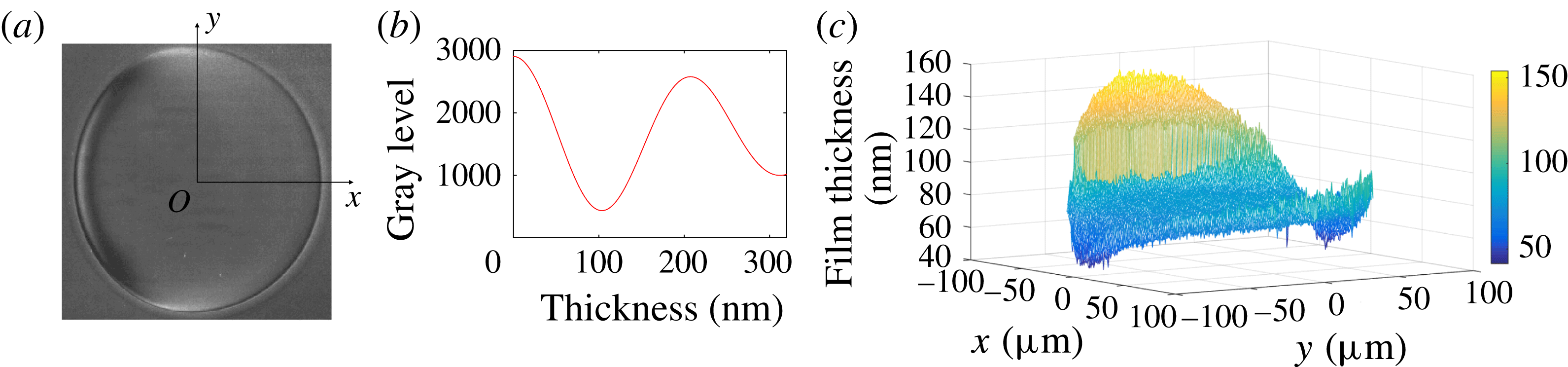
. (b) Theoretical variation of the reflected light intensity with the film thickness (the optical model is detailed in Huerre et al. (Reference Huerre, Jullien, Theodoly and Valignat2016)). (c) Film topography extracted from image (a).
The topography of the lubrication film is measured at the bottom wall, below the moving droplet, using RICM (figure 1
b). This technique has been covered in detail in a previous article, and only the main steps are mentioned here (see Huerre et al.
Reference Huerre, Jullien, Theodoly and Valignat2016). Light is provided by an X-Cite 120Q lamp with an RGB filter (Semrock: FF01 – 464/542/639 nm), so that the intensity is high enough to investigate faster droplets, compared to the previous work. Experimental movies are acquired using a high-speed camera (Photron) at 250 Hz and a Zeiss Neofluar 63/1.25 antiflex objective. The pixel resolution is
 $\unicode[STIX]{x1D6FF}_{pix}=0.67~\unicode[STIX]{x03BC}\text{m}^{-1}$
. A raw RICM picture of a travelling droplet moving from left to right is shown in figure 2(a). Contrasted grey levels are observed within the thin film, whereas the static meniscus corresponds to a uniform grey level: this well-defined transition provides an experimental definition of the frontier between the thin film of radius
 $R$
and the unresolved meniscus. The film thickness is determined with high accuracy from the RICM picture, to a precision of 4 nm, using the relationship between the light intensity and the film thickness given in figure 2(b). The detail of the image processing is given in appendix A. A height difference of 100 nm corresponds to one half intensity oscillation: if the film thickness varies for more than 100 nm over a single pixel, the signal is lost, as happens outside the central disc in figure 2(a), and an average grey level is measured. The region we are able to characterize is represented in figure 1(c).
2.2 Notes on the experiments
We first reported experimental evidence of 3D topographies of the lubrication film using a similar experimental set-up in a previous work (Huerre et al. Reference Huerre, Theodoly, Leshansky, Valignat, Cantat and Jullien2015). The present work aims to investigate these 3D geometries more locally. As listed below, the physicochemical properties of the solution we choose belongs a priori to the class of systems leading to stress-free interfaces. However, even in this model situation, we show that strong surfactant effects are observed in some domains on the interface.
(i) First, Park & Homsy (Reference Park and Homsy1984) showed that the viscosity of the droplet has a negligible influence on the film thickness, as long as the viscosity ratio between the inner and outer phases remains smaller than
 $Ca^{-1/3}$
. In our experimental conditions, we set
$\unicode[STIX]{x1D702}_{i}/\unicode[STIX]{x1D702}_{o}=0.256$
and
$Ca^{-1/3}=7$
at the highest velocity explored, so that additional effects due to droplet viscosity are expected to be negligible.
(ii) Secondly, Bretherton’s model assumes a stress-free boundary condition, but an interface viscosity or elasticity can induce a thickening of the lubrication film by a factor of up to 2.5 (Quéré & de Ryck Reference Quéré and de Ryck1998; Shen et al. Reference Shen, Gleason, McKinley and Stone2002; Scheid et al. Reference Scheid, Delacotte, Dollet, Rio, Restagno, van Nierop, Cantat, Langevin and Stone2010; Delacotte et al. Reference Delacotte, Montel, Restagno, Scheid, Dollet, Stone, Langevin and Rio2012; Champougny et al. Reference Champougny, Scheid, Restagno, Vermant and Rio2015). We chose to use a surfactant (C
$_{10}$
TAB) that was previously shown to have negligible influence on the boundary condition by Delacotte et al. (Reference Delacotte, Montel, Restagno, Scheid, Dollet, Stone, Langevin and Rio2012), in similar experimental conditions: same solution (without salt), same capillary range, but larger scale (meniscus size).(iii) In the range of confinement that is investigated using microfluidics, the thin liquid film squeezed between the droplet and the wall may be so thin that intermolecular interactions come into play and may set the lubrication film thickness (Huerre et al. Reference Huerre, Theodoly, Leshansky, Valignat, Cantat and Jullien2015). In order to screen the electrostatic contribution of the disjoining pressure, the Debye layers are screened by adding salt in the external phase such that the Debye length is reduced to
$\unicode[STIX]{x1D706}_{D}=0.2~\text{nm}$
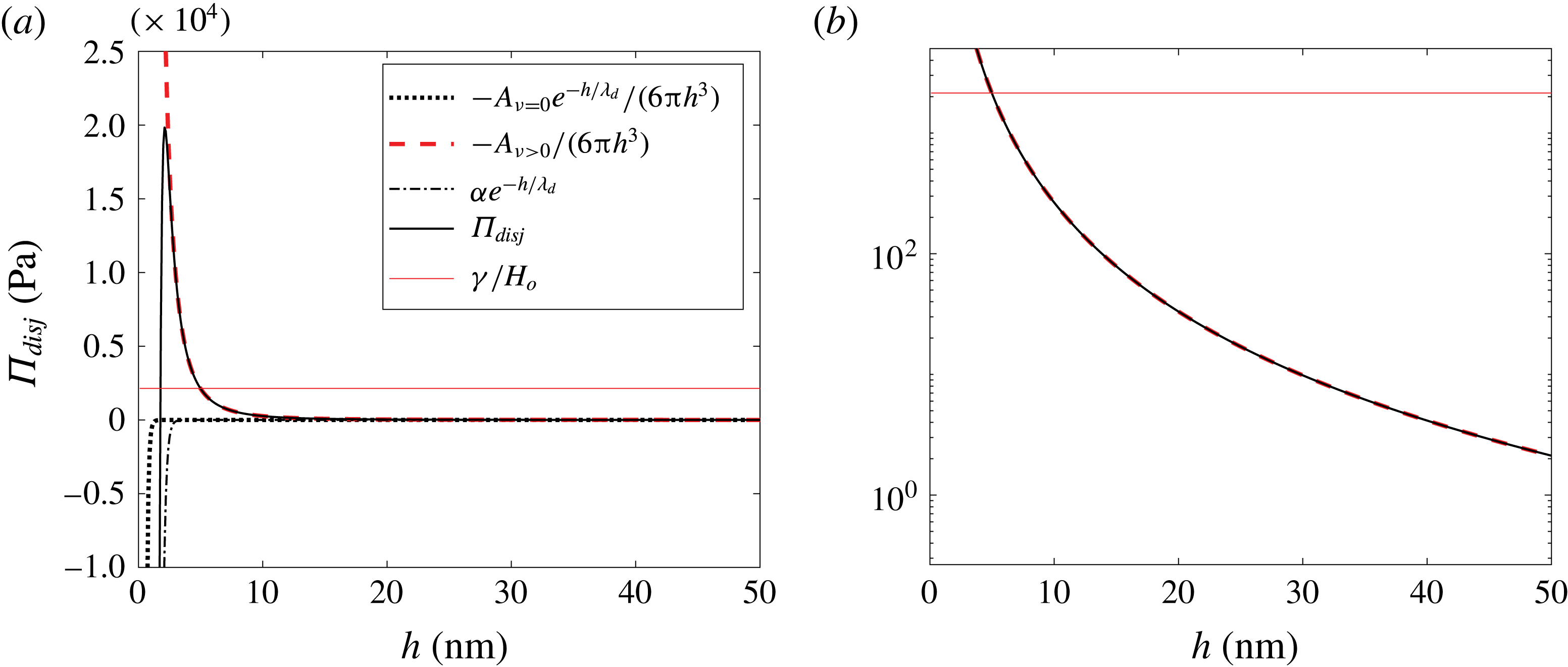
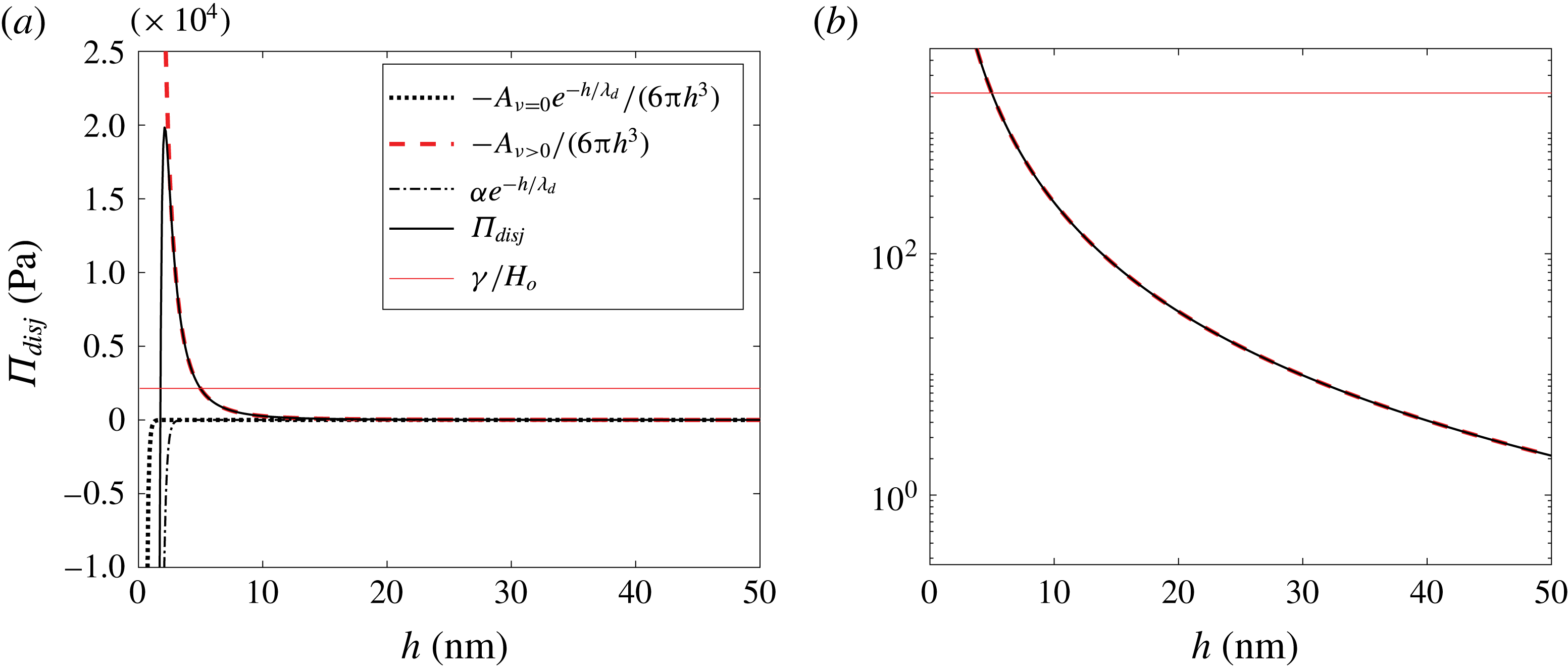
. The intermolecular interaction is thus governed by the dispersion contribution of the van der Waals interactions. In appendix C, we show that, in the range of scales that are measured in the reported experiment, the film thickness is governed by hydrodynamics, and that disjoining pressure effects can be comfortably neglected. This effect will be neither considered nor discussed in the following.


As a whole, care has been taken in order to fulfill a priori stress-free boundary conditions, for a droplet of negligible viscous effect, and for which intermolecular effects lie within the error bars.
3 Geometry and film domains
The geometry of the film is described in the droplet reference frame
 $(O,\boldsymbol{e}_{x},\boldsymbol{e}_{y},\boldsymbol{e}_{z})$
. The origin
 $O$
sits at the centre of the film in the bottom wall plane
 $(x,y)$
, with
 $-x$
the direction of wall motion, and
 $z$
the normal to the wall oriented upwards. Polar coordinates
 $(\unicode[STIX]{x1D70C},\unicode[STIX]{x1D703},z)$
are used, with a polar axis in the
 $x$
direction. And
 $h(x,y)$
is the film thickness, between the bottom wall and the liquid–liquid interface (see figure 1
c).
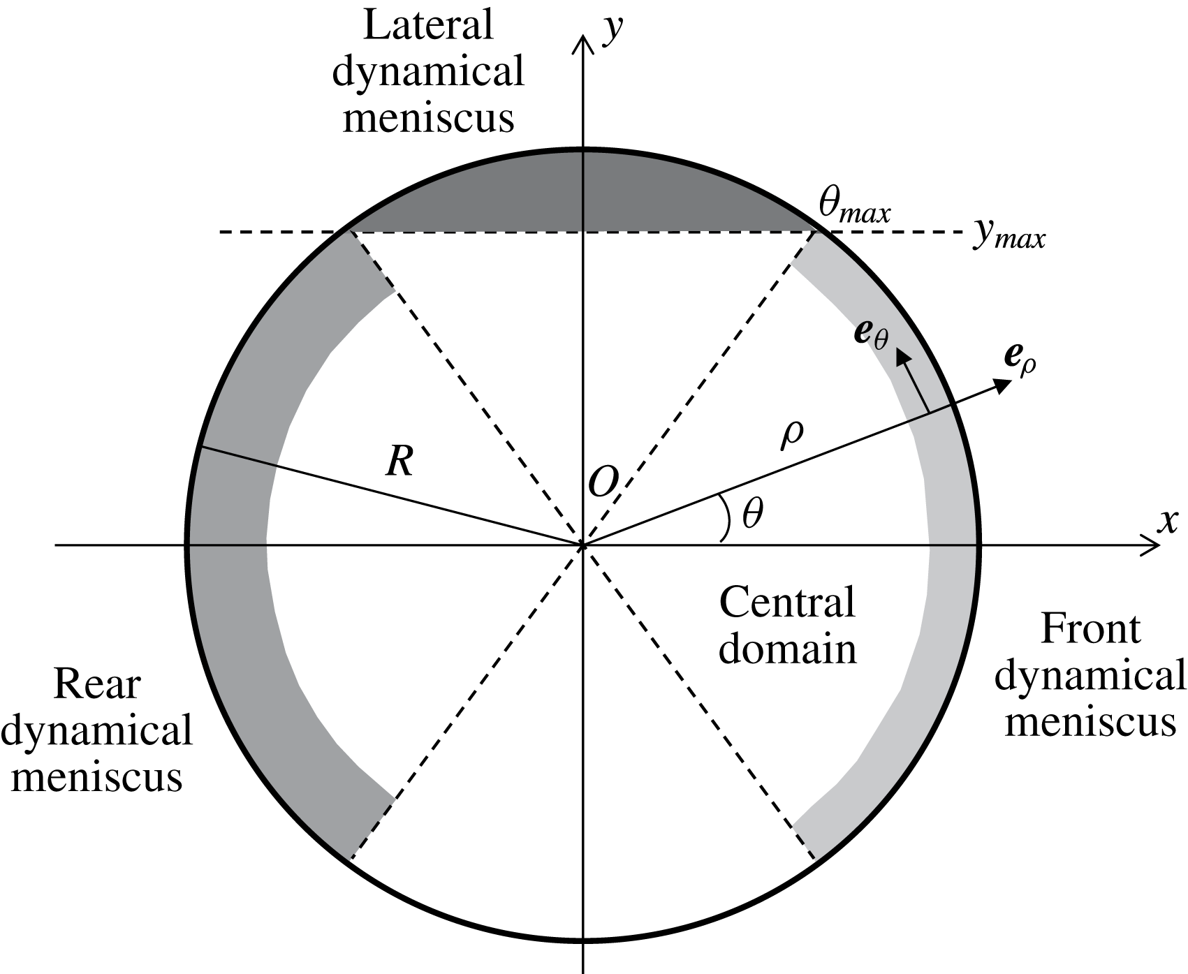
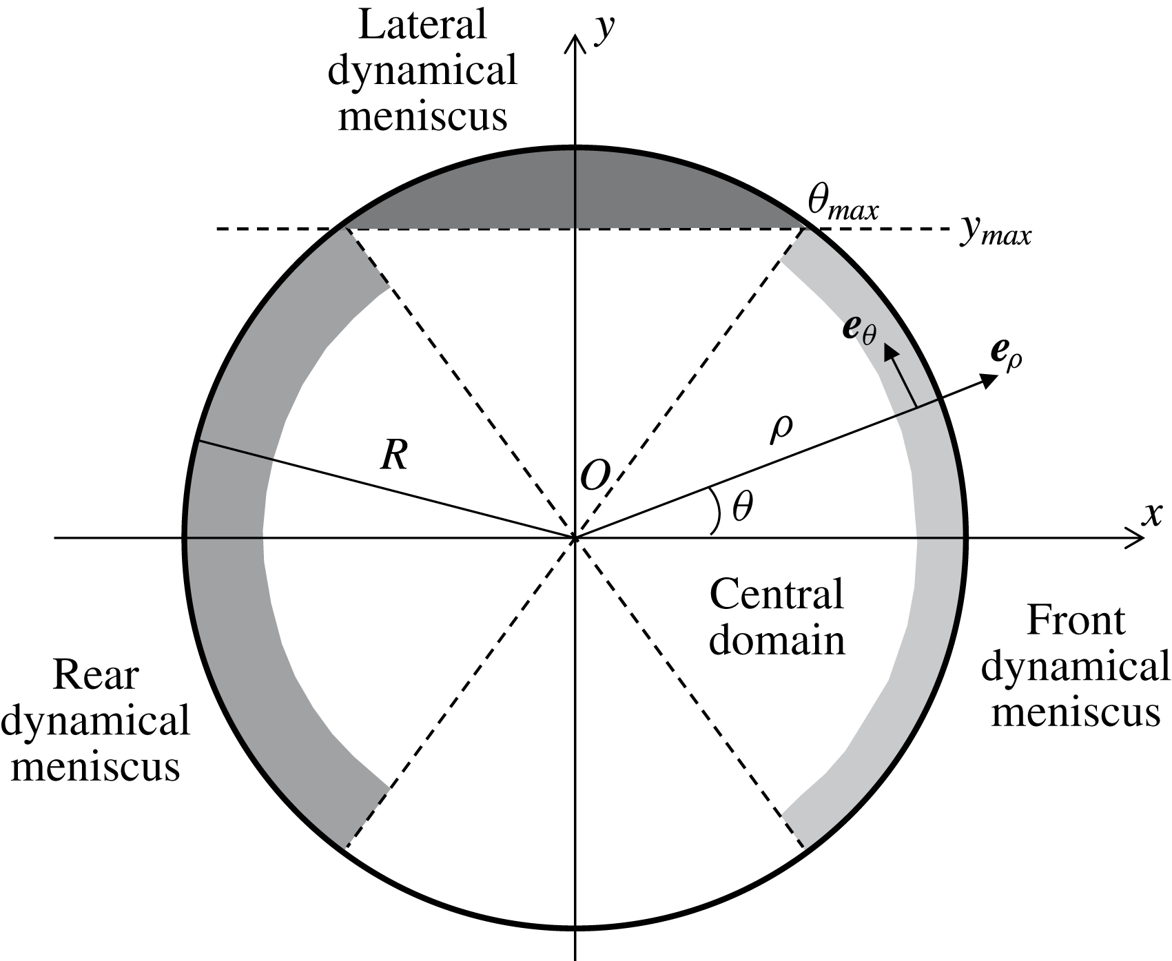
Definition of the geometrical parameters and of the separate domains in the lubrication film. The disc of radius
 $R$
corresponds to the region where
 $h(x,y)$
can be measured, and is divided into the front and rear meniscus domains, the central domain and the two lateral meniscus domains, represented using different grey levels. For clarity, the radial extension of the dynamical menisci are oversized.
At first glance, the contour of the thin film is almost circular, with relative variations of its radius of order
 $\unicode[STIX]{x1D6FF}R/R\sim 3\,\%$
, the in-plane curvature being slightly smaller at the rear than at the front. The corresponding Laplace pressure variation scales as
 $\unicode[STIX]{x1D6FF}P=\unicode[STIX]{x1D6FE}\unicode[STIX]{x1D6FF}R/R^{2}\sim 5~\text{Pa}$
. This is consistent with the order of magnitude of the viscous pressure field
 $(\unicode[STIX]{x1D702}_{o}-\unicode[STIX]{x1D702}_{i})U_{d}R/H_{0}^{2}\sim 18~\text{Pa}$
, responsible for this deformation at the droplet scale. We neglect it in what follows, and assume that the thin film is a disc of radius
 $R$
while the lateral droplet interface keeps its static equilibrium shape, with a total curvature close to
 $1/H_{o}$
.
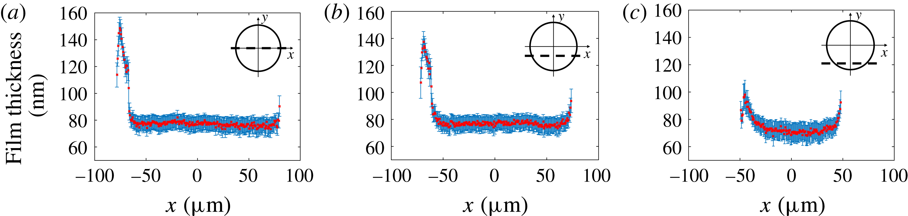
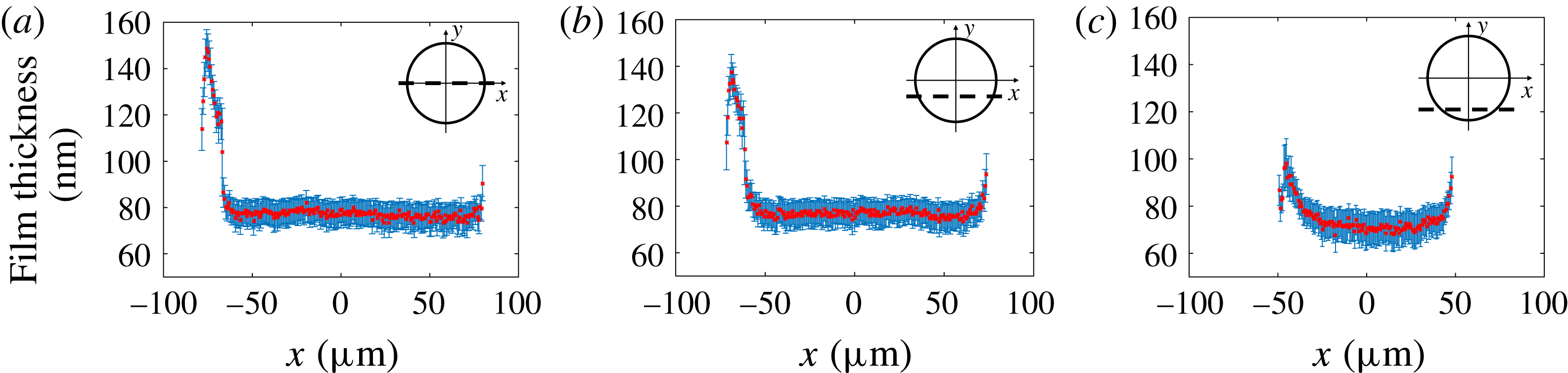
The film topography extracted from the RICM picture in figure 2(a) is plotted in figure 2(c). It shows a complex catamaran-like 3D shape, with a bump at the rear and two ravines on the sides, as previously observed by Huerre et al. (Reference Huerre, Jullien, Theodoly and Valignat2016). To address the complexity of this shape, the film is decomposed into four parts, shown in figure 3 and analysed independently: (i) the central region, (ii) the front dynamical meniscus, (iii) the rear dynamical meniscus and (iv) the lateral dynamical meniscus. Figure 4 shows longitudinal film profiles taken at different values of
 $y$
for a given
 $Ca$
. Far enough from the front and rear menisci, the film thickness keeps a value independent of
 $x$
,
 $h_{\infty }(y)$
, that can be defined without ambiguity for
 $|y|<y_{max}=R\sin (\unicode[STIX]{x1D703}_{max})$
; see figure 3. This angle, of order
 $\unicode[STIX]{x1D703}_{max}\sim 1.2$
for all
 $Ca$
, allows us to define experimentally the frontier to the lateral meniscus: with this convention
 $y_{max}=0.92R$
. In turn, the region where
 $h(x,y)=h_{\infty }(y)$
is referred to as the central region, or flat film.
Longitudinal profiles of the film thickness
 $h(x,y)$
, along the lines (a)
 $y=0~\unicode[STIX]{x03BC}\text{m}$
, (b)
 $y=-34~\unicode[STIX]{x03BC}\text{m}$
(
 $|y|=0.4R$
) and (c)
 $y=-68~\unicode[STIX]{x03BC}\text{m}$
(
 $|y|=0.8R$
). The capillary number is
 $Ca=7.2\times 10^{-4}$
. Insets: the dashed line indicates the location of the longitudinal profile for each
 $y$
value.
4 Longitudinal film profiles for
$y=0$

4.1 2D theoretical framework
Bretherton’s classical result is established for the configuration shown in figure 1(c), for a droplet invariant along
 $y$
and of negligible viscosity. The flow in the thin film is determined using the lubrication approximation
 $\unicode[STIX]{x2202}p/\unicode[STIX]{x2202}x=\unicode[STIX]{x1D702}_{o}(\unicode[STIX]{x2202}^{2}u/\unicode[STIX]{x2202}z^{2})$
, where the pressure
 $p$
does not depend on
 $z$
and
 $u$
is the
 $x$
component of the velocity field in the droplet’s frame. Continuity of the normal stress at the interface imposes a Laplace pressure difference
 $p_{o}-p=\unicode[STIX]{x1D6FE}\unicode[STIX]{x2202}^{2}h/\unicode[STIX]{x2202}x^{2}$
, where
 $p_{o}$
is the uniform internal pressure within the droplet. The boundary conditions
 $u(z=0)=-U_{d}$
and
 $u(z=h)=u_{s}(x)$
give the velocity profile:
 $$\begin{eqnarray}u(x,z)=\frac{\unicode[STIX]{x1D6FE}}{2\unicode[STIX]{x1D702}_{o}}\frac{\unicode[STIX]{x2202}^{3}h}{\unicode[STIX]{x2202}x^{3}}(h-z)z+\frac{(u_{s}+U_{d})}{h}z-U_{d}.\end{eqnarray}$$
At the front meniscus, in the small-
 $x$
limit, a flat film of unknown thickness
 $h=h_{\infty }$
is assumed, as well as a constant interfacial velocity
 $u_{s}^{0}$
. The velocity field in this film is therefore given by
 $u=((u_{s}^{0}+U_{d})/h_{\infty })z-U_{d}$
, and the flow rate
 $Q(x)=\int _{0}^{h}u\,\text{d}z$
becomes
 $Q_{0}=h_{\infty }(u_{s}^{0}-U_{d})/2$
. For an incompressible and steady flow, writing
 $Q(x)=Q_{0}$
gives
 $$\begin{eqnarray}-\!\unicode[STIX]{x1D6FE}\frac{\unicode[STIX]{x2202}^{3}h}{\unicode[STIX]{x2202}x^{3}}=\frac{6\unicode[STIX]{x1D702}_{o}}{h^{3}}[h(u_{s}-U_{d})-h_{\infty }(u_{s}^{0}-U_{d})].\end{eqnarray}$$
Additionally, the continuity of the tangential stress at the interface leads to the following Marangoni relation,
 $$\begin{eqnarray}\frac{\unicode[STIX]{x2202}\unicode[STIX]{x1D6FF}\unicode[STIX]{x1D6FE}}{\unicode[STIX]{x2202}x}=\unicode[STIX]{x1D702}_{o}\frac{\unicode[STIX]{x2202}u}{\unicode[STIX]{x2202}z}(h),\end{eqnarray}$$
with
 $\unicode[STIX]{x1D6FF}\unicode[STIX]{x1D6FE}$
the interfacial stress variation relative to its reference value
 $\unicode[STIX]{x1D6FE}$
. Equation (4.2) is general, in the sense that it is valid for any rheological properties of the interface, as long as
 $\unicode[STIX]{x1D6FF}\unicode[STIX]{x1D6FE}\ll \unicode[STIX]{x1D6FE}$
.
In his study, Bretherton imposes a stress-free condition, i.e.
 $\unicode[STIX]{x1D6FF}\unicode[STIX]{x1D6FE}=0$
. The corresponding boundary condition at the interface,
 $\unicode[STIX]{x2202}u/\unicode[STIX]{x2202}z=0$
, then yields
 $u_{s}=-U_{d}+(\unicode[STIX]{x1D6FE}/2\unicode[STIX]{x1D702}_{o})(\unicode[STIX]{x2202}^{3}h/\unicode[STIX]{x2202}x^{3})h^{2}$
and
 $u_{s}^{0}=-U_{d}$
. By substituting these two expressions in (4.2), Bretherton’s classical equation is recovered:
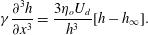 $$\begin{eqnarray}\unicode[STIX]{x1D6FE}\frac{\unicode[STIX]{x2202}^{3}h}{\unicode[STIX]{x2202}x^{3}}=\frac{3\unicode[STIX]{x1D702}_{o}U_{d}}{h^{3}}[h-h_{\infty }].\end{eqnarray}$$
Finally, we impose a curvature
 $1/H_{o}$
at large
 $x$
to solve this equation numerically and write the thickness in the flat film:
 $$\begin{eqnarray}h^{Breth}=1.337H_{o}Ca^{2/3}.\end{eqnarray}$$
To derive the profile in the rear meniscus, the same approach is used. However, the problem is not symmetric with respect to the
 $y$
axis in terms of boundary conditions. At the front meniscus
 $x\geqslant 0$
and the curvature is set to
 $1/H_{0}$
at large
 $x$
. However, at the rear meniscus,
 $x\leqslant 0$
and there are two constraints to ensure the uniqueness of the solution: setting the curvature equal to
 $1/H_{0}$
at small
 $x$
, and an asymptotic film thickness at large
 $x$
. This leads to a monotonic evolution of the profile at the front and to an oscillation in the rear meniscus.
4.2 Front meniscus and central region
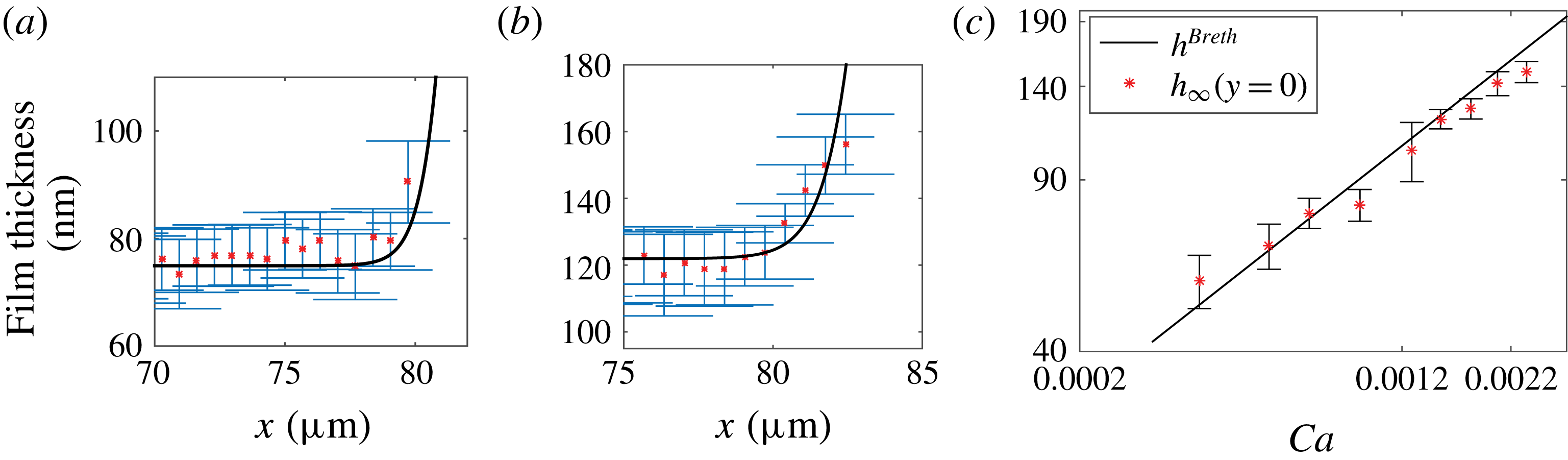
Examples of film profiles close to the front meniscus along the
 $x$
axis and for
 $y=0$
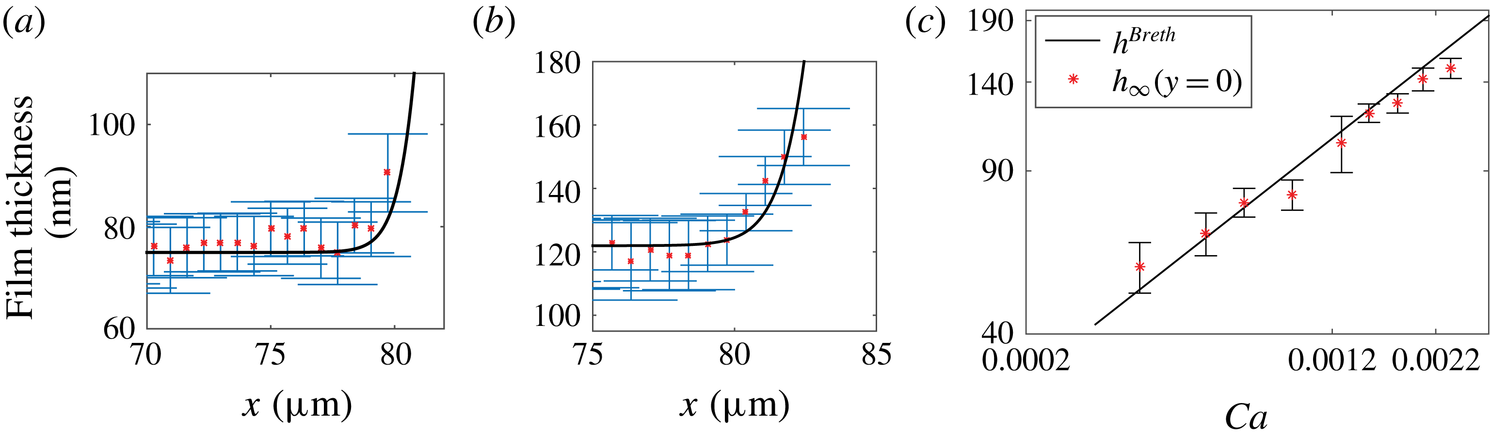
are given in figure 5(a,b). These experimental profiles are in quantitative agreement with numerical solutions of (4.4) for a meniscus of curvature
 $1/H_{o}$
at large
 $x$
. In particular, we recover
 $h_{\infty }(y=0)=h^{Breth}$
from (4.5), within the precision of our error bars, over the whole range of capillary numbers investigated (figure 5
c). This confirms that the additional contributions that we aimed to keep negligible, such as droplet viscosity, disjoining pressure or surfactant effects, do not affect the profile significantly in this region of the droplet, where Bretherton’s model correctly captures the film thickness.
Front meniscus profile and film height in the central region. Film profiles
 $h(x,y)$
along the
 $x$
axis (
 $y=0$
) for (a)
 $Ca=7.2\times 10^{-4}$
and (b)
 $Ca=1.5\times 10^{-3}$
. Solid line: Bretherton’s prediction from (4.4). (c) Variation of
 $h_{\infty }(y=0)$
with
 $Ca$
. Solid line: Bretherton’s solution,
 $h^{Breth}=1.337H_{o}Ca^{2/3}$
.
Regarding the non-axisymmetric geometry, Burgess & Foster (Reference Burgess and Foster1990) found under similar assumptions that the 2D prediction for the film thickness remains valid in the
 $(x,O,z)$
plane as long as
 $(H_{o}/R)^{3}\ll Ca\ll H_{o}/R\ll 1$
, which was confirmed numerically by Zhu & Gallaire (Reference Zhu and Gallaire2016). In our case the constraint
 $(H_{o}/R)^{3}\ll Ca$
is not fully satisfied at our smallest capillary numbers, and a geometrical correction to the meniscus curvature might be expected. The Laplace pressure drop, at the droplet interface, at equilibrium is given by (de Laplace Reference de Laplace1806)
 $$\begin{eqnarray}\unicode[STIX]{x0394}P=\unicode[STIX]{x1D6FE}\left(\frac{1}{R_{1}}+\frac{1}{R_{2}}\right)=\frac{\unicode[STIX]{x1D6FE}}{H_{o}}\left(1+\frac{\unicode[STIX]{x03C0}}{4}\frac{H_{0}}{R}\right),\end{eqnarray}$$
with
 $R_{1}$
and
 $R_{2}$
the two principal radii of curvature of the interface. As one principal curvature is zero at the contact with the wall, this relation gives us the radius of curvature of the meniscus near the transition to the flat film:
 $r^{\ast }=H_{o}(1-\unicode[STIX]{x03C0}H_{o}/(4R))=H_{o}(1-0.06)$
at the first order in
 $H_{o}/R$
. Using
 $r^{\ast }$
instead of
 $H_{o}$
in (4.5) gives a correction to the film thickness of order
 $Ca^{2/3}H_{o}/R$
, neglected in Burgess & Foster (Reference Burgess and Foster1990). Here, this correction is approximately 6 % and lies within the experimental error bar. For this reason, further comparisons with the theory are made using a meniscus curvature of
 $1/H_{o}$
.
4.3 Rear meniscus
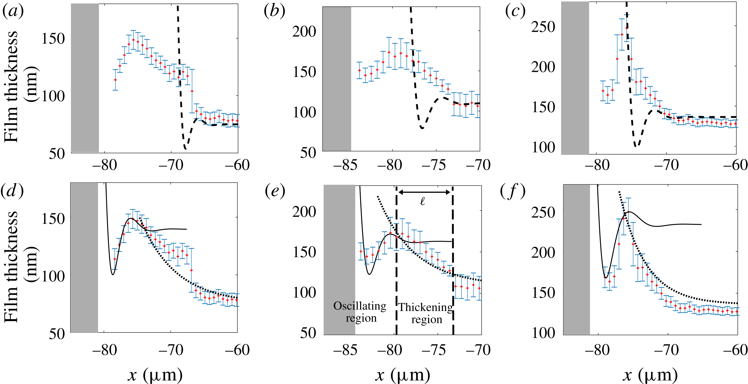
As shown in figure 6, the transition between the central part of the film and the rear meniscus is characterized by a non-monotonic variation of the film thickness, in contrast to the behaviour at the front of the droplet. The determination of the film thickness, from the images, in this region is thus delicate and is discussed in appendix A. When approaching the rear meniscus from the flat film along the
 $x$
axis, the film thickness first increases towards a maximum value
 $h_{max}$
, then decreases, before finally diverging when reaching the meniscus. The minimum thickness, located between the bump at
 $h_{max}$
and the rear meniscus, is not resolved on all images and its value is therefore not reported in this paper. Indeed, around the minimum, the film thickness varies so fast that an average grey level is obtained on the images. Consequently, the position of the minimum is resolved within one pixel whereas the film thickness value is not resolved. On the graphs the unresolved meniscus is symbolized by a grey zone (see figure 6).
Oscillation at the rear meniscus. Longitudinal thickness profiles for three increasing values of
 $Ca$
: (a,d)
 $Ca=7.2\times 10^{-4}$
, (b,e)
 $Ca=1.3\times 10^{-3}$
and (c,f)
 $Ca=1.8\times 10^{-3}$
. The film thickness at large
 $x$
is
 $h_{\infty }(0)$
and the local maximum is
 $h_{max}$
. Dashed lines in (a–c) show Bretherton’s prediction from (4.4). Dotted lines in (d–f) show film profile deduced using the surfactant mass transport model ((4.16) with
 $Ma=1.6$
). Solid lines in (d–f) show theoretical predictions from (4.18) using
 $u_{s}^{max}=U_{d}(1-2h_{\infty }(0)/h_{max})$
. The grey zone symbolizes the unresolved meniscus.
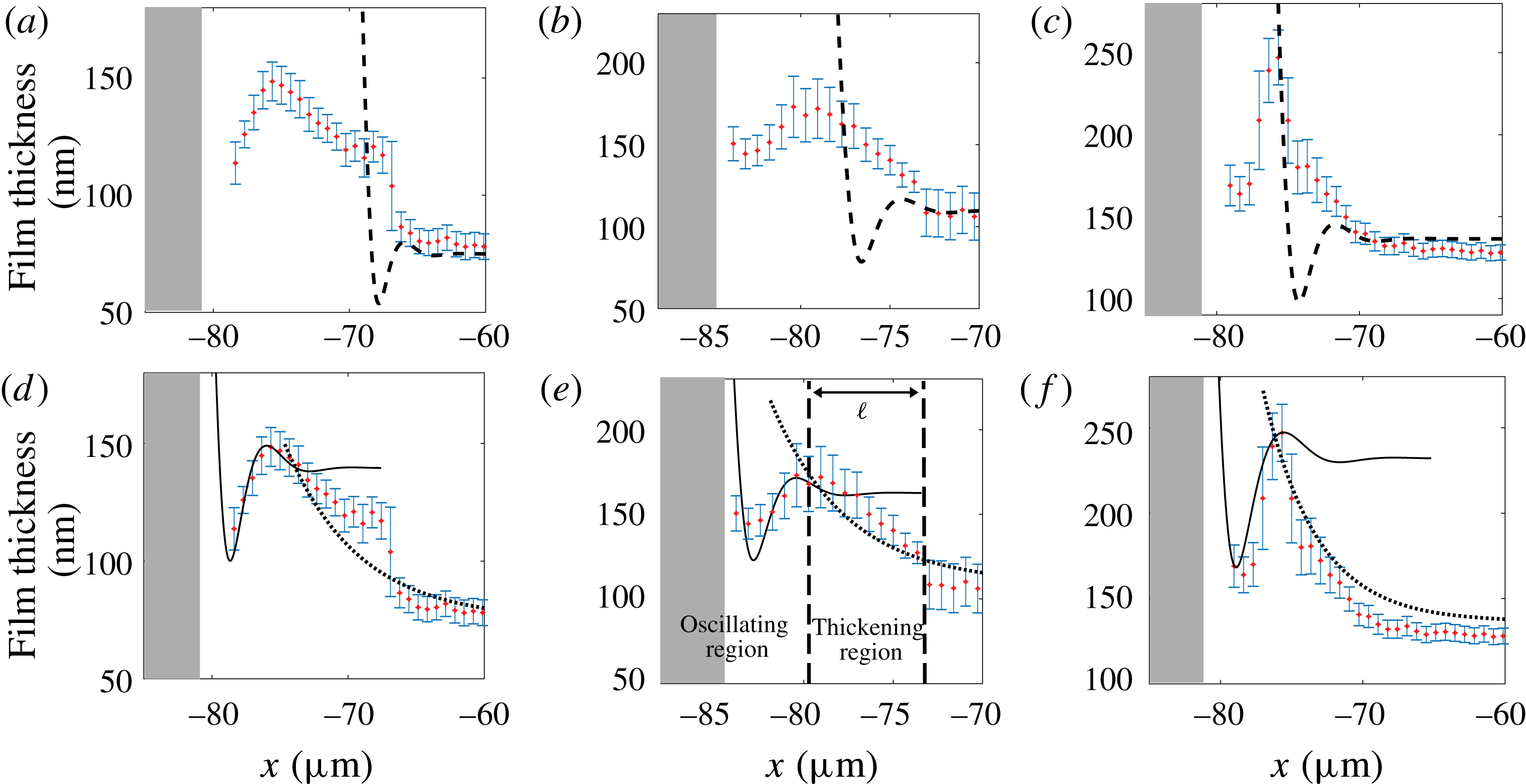
Given the very good agreement found at the front meniscus, these experimental profiles are first compared to Bretherton’s prediction for the rear meniscus, i.e. the solution of (4.4) for a stress-free boundary condition, with a curvature
 $1/H_{o}$
at small
 $x$
and a flat film of thickness
 $h^{Breth}$
at large
 $x$
. Surprisingly, we find that the experimental profiles of the rear meniscus are very far from the theory (see figure 6
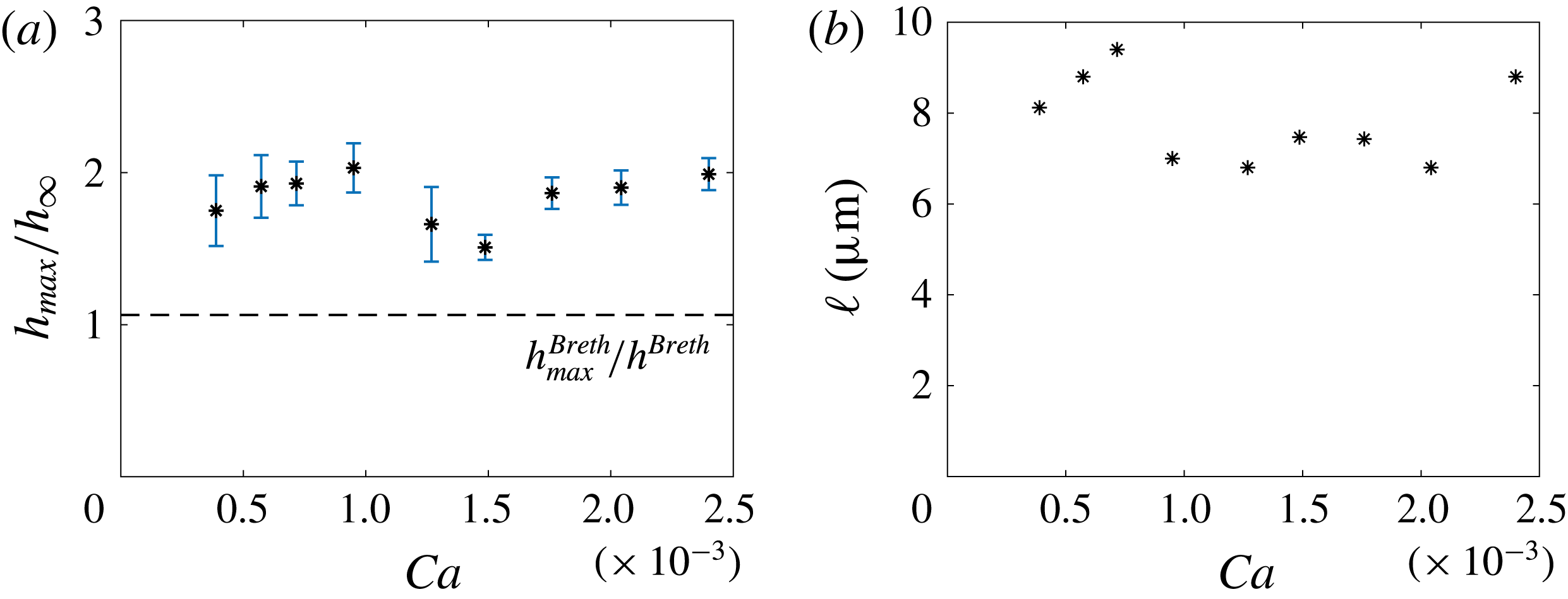
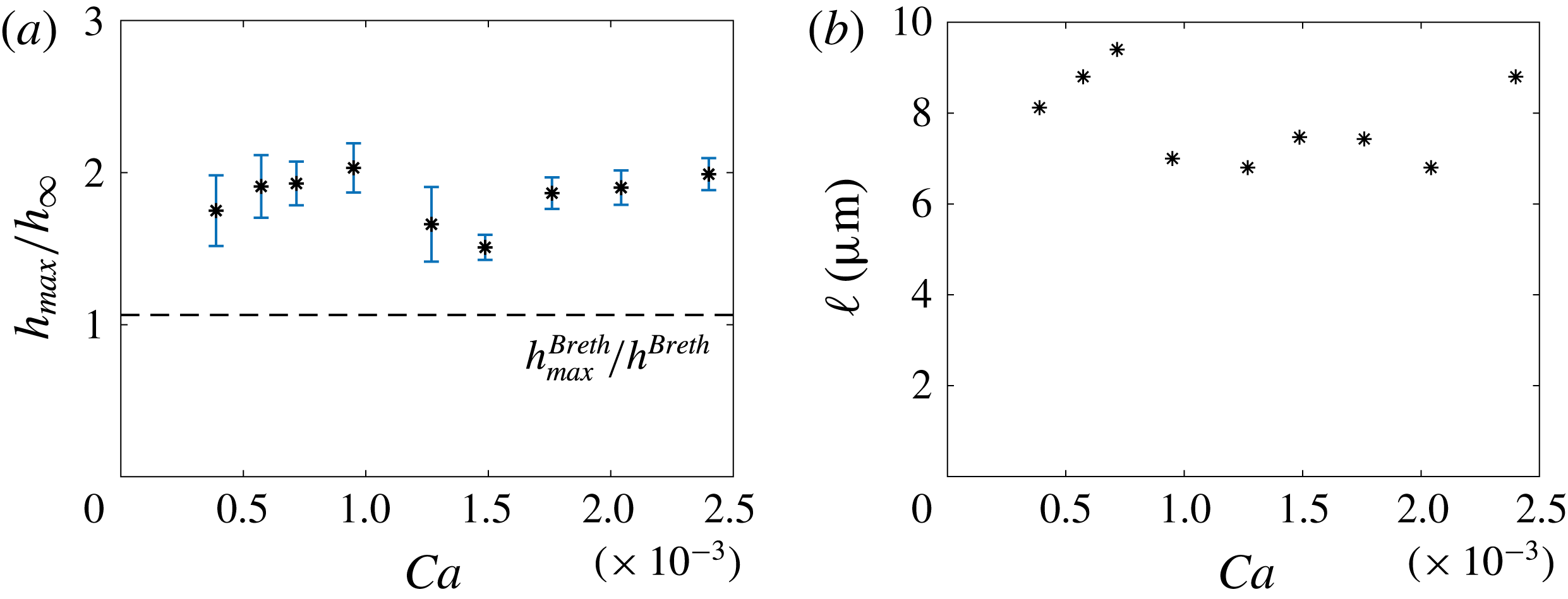
a–c). The ratio
 $h_{max}/h_{\infty }(y=0)$
is plotted in figure 7(a): we measure
 $h_{max}/h_{\infty }(y=0)\simeq 1.7$
for all capillary numbers, whereas the prediction for a stress-free interface is
 $h_{max}^{Breth}/h^{Breth}=1.064$
. Similarly, the distance
 $\ell$
over which the film thickening develops (see figure 6
e) is found to be
 $7.5~\unicode[STIX]{x03BC}\text{m}$
, whatever the capillary number (see figure 7
b) and is much larger than the value predicted by Bretherton’s model. The rear bump predicted by Bretherton’s model is governed by the Laplace pressure induced by the capillary suction in the meniscus. As our experimental value of the bump height
 $(h_{max}-h_{\infty }(0))$
is one order of magnitude larger than Bretherton’s prediction, this thickening must arise from another physical phenomenon.
(a) Maximum height at the bump, relative to the height in the flat film. (b) Length of the thickening region
 $\ell$
as a function of the capillary number
 $Ca=\unicode[STIX]{x1D702}_{o}U_{d}/\unicode[STIX]{x1D6FE}$
.
It is well known for spherical bubbles rising in a surfactant solution that surfactants accumulate at the rear and rigidify the interface. If the diffusion is slow enough in comparison with convection, the Marangoni effect leads to the stagnant-cap regime: the interface velocity is the bubble velocity on a spherical cap at the rear, whereas the stress-free condition still applies on the remaining part of the interface (Cuenot, Magnaudet & Spennato Reference Cuenot, Magnaudet and Spennato1997). In confined situations Park (Reference Park1992) and Cantat & Dollet (Reference Cantat and Dollet2012) show that stiffening can actually lead to a thickening factor equal to 2 if the interface velocity reaches the rear meniscus velocity (full stiffening).
In the following, we propose a model to predict the film profile observed at the rear. Similarly to the front region, the system is almost invariant in the
 $y$
direction close to the
 $x$
axis, and we use a 2D model. The rear meniscus domain is split into two regions: a thickening region between the flat film and the rear bump, and an oscillating region (see figure 6
e). In the first one, the Laplace pressure is neglected on the basis of the previous analysis, and the surfactant transport is solved. In the second, a full stiffening of the interface is assumed and the lubrication equations are solved, with Laplace pressure. These simplified approaches allow one to reproduce the observed profiles and thus to identify the dominant physical ingredients in each region.
The dominant term of the transport equation is determined on the basis of the following characteristic times: the diffusion time along the
 $x$
direction based on the distance
 $\ell$
,
 $t_{d1}=\ell ^{2}/D=5\times 10^{-2}~\text{s}$
(
 $D=10^{-9}~\text{m}^{2}~\text{s}^{-1}$
); the diffusion time in the
 $z$
direction,
 $t_{d2}=h_{\infty }^{2}/D=10^{-5}~\text{s}$
(
 $h_{\infty }=10^{-7}~\text{m}$
); the sorption kinetic characteristic time
 $t_{s}=\unicode[STIX]{x1D6E4}_{\infty }/(kc_{o})=3\times 10^{-7}~\text{s}$
(
 $\unicode[STIX]{x1D6E4}_{\infty }\simeq 3\times 10^{-6}~\text{mol}~\text{m}^{-2}$
is the interfacial concentration on the film and
 $k\simeq 10^{-2}~\text{m}~\text{s}^{-1}$
(Quéré & de Ryck Reference Quéré and de Ryck1998)); and the characteristic convection time
 $t_{c}=\ell /U_{d}=7\times 10^{-3}~\text{s}$
(
 $U_{d}=10^{-3}~\text{m}~\text{s}^{-1}$
). As both
 $t_{s}$
and
 $t_{d2}$
are much smaller than
 $t_{c}$
and
 $t_{d1}$
, the bulk concentration is homogeneous over
 $z$
and is in equilibrium with the interface concentration. Conversely,
 $t_{d1}$
is much larger than
 $t_{c}$
, and axial diffusion is thus small compared to axial convection. For these two reasons, the diffusive processes can be scaled out. In this limit the transport equation only depends on convection and can be obtained by a simple mass balance in a fluid slice located between
 $x$
and
 $x+\text{d}x$
.
In steady state the interfacial concentration
 $\unicode[STIX]{x1D6E4}$
is given by surfactant mass conservation along the
 $x$
direction,
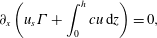 $$\begin{eqnarray}\unicode[STIX]{x2202}_{x}\left(u_{s}\unicode[STIX]{x1D6E4}+\int _{0}^{h}cu\,\text{d}z\right)=0,\end{eqnarray}$$
with
 $c$
the bulk concentration. The latter,
 $c$
, does not depend on
 $z$
, as discussed before, and using the mass conservation
 $\int _{0}^{h}u\,\text{d}z=-U_{d}h_{\infty }$
, equation (4.7) is integrated to
 $$\begin{eqnarray}u_{s}\unicode[STIX]{x1D6E4}=-U_{d}\unicode[STIX]{x1D6E4}_{\infty }+(c-c_{\infty })U_{d}h_{\infty },\end{eqnarray}$$
with
 $c_{\infty }$
and
 $\unicode[STIX]{x1D6E4}_{\infty }$
the bulk and interface concentrations in the film, far from the thickening region.
Assuming a linear sorption law (Brenner Reference Brenner2013) and fast sorption kinetics, the interfacial concentration is in equilibrium with the bulk concentration
 $c$
:
 $$\begin{eqnarray}\frac{\unicode[STIX]{x1D6E4}}{c}=\frac{\unicode[STIX]{x1D6E4}_{\infty }}{c_{\infty }}=h_{\unicode[STIX]{x1D6E4}},\end{eqnarray}$$
for
 $\unicode[STIX]{x1D6E4}_{\infty }=3\times 10^{-6}~\text{mol}~\text{m}^{-2}$
and
 $c_{\infty }=c_{o}=10^{3}~\text{mol}~\text{m}^{-3}$
,
 $h_{\unicode[STIX]{x1D6E4}}\simeq 3~\text{nm}$
.
Finally, in the absence of Laplace pressure, (4.2) simplifies to
 $$\begin{eqnarray}u_{s}(x)=U_{d}\left[1-\frac{2h_{\infty }(0)}{h(x,0)}\right].\end{eqnarray}$$
The interfacial velocity in the wetting film can vary between
 $u_{s}=-U_{d}$
, i.e. the wall velocity, in the stress-free case (assumed at the front) and
 $u_{s}=0$
, i.e. the velocity of the rear meniscus, in the fully stiffened case. The film thickness is thus in the range
 $[h_{\infty };2h_{\infty }]$
, or equivalently the thickening factor due to Marangoni effects at the rear ranges from 1 to 2. The velocity profile in the film is linear and (4.3) becomes, for small tension variations,
 $$\begin{eqnarray}\unicode[STIX]{x1D702}_{o}\frac{u_{s}+U_{d}}{h}=-|\unicode[STIX]{x2202}_{\unicode[STIX]{x1D6E4}}\unicode[STIX]{x1D6FE}|\frac{\unicode[STIX]{x2202}\unicode[STIX]{x1D6E4}}{\unicode[STIX]{x2202}x}.\end{eqnarray}$$
Equations (4.8)–(4.11) constitute a closed set of equations for the unknown functions
 $h$
,
 $u_{s}$
,
 $c$
and
 $\unicode[STIX]{x1D6E4}$
, solved in the following. Introducing the Marangoni number
 $Ma=|\unicode[STIX]{x2202}_{\unicode[STIX]{x1D6E4}}\unicode[STIX]{x1D6FE}|\unicode[STIX]{x1D6E4}_{\infty }/\unicode[STIX]{x1D6FE}$
and
 $K=h_{\infty }/h_{\unicode[STIX]{x1D6E4}}$
, we use the dimensionless variables
 $u_{s}=\hat{U} U_{d}$
,
 $x=2\hat{X}h_{\infty }Ma/(KCa)$
,
 $h=h_{\infty }{\hat{H}}$
and
 $\unicode[STIX]{x1D6E4}=\hat{\unicode[STIX]{x1D6E4}}\unicode[STIX]{x1D6E4}_{\infty }$
. Equations (4.8), (4.10) and (4.11) become
 $$\begin{eqnarray}\displaystyle & \displaystyle \hat{U} \hat{\unicode[STIX]{x1D6E4}}=-1+(\hat{\unicode[STIX]{x1D6E4}}-1)K, & \displaystyle\end{eqnarray}$$
 $$\begin{eqnarray}\displaystyle & \displaystyle \frac{2}{{\hat{H}}}=1-\hat{U} , & \displaystyle\end{eqnarray}$$
 $$\begin{eqnarray}\displaystyle & \displaystyle \frac{1+\hat{U} }{{\hat{H}}}=-K\unicode[STIX]{x2202}_{\hat{X}}\hat{\unicode[STIX]{x1D6E4}}/2. & \displaystyle\end{eqnarray}$$
Substitution leads to an equation in
 $\hat{U}$
only:
 $$\begin{eqnarray}\unicode[STIX]{x2202}_{\hat{X}}\hat{U} =\frac{(\hat{U} ^{2}-1)(K-\hat{U} )^{2}}{K(1+K)}\simeq (\hat{U} ^{2}-1).\end{eqnarray}$$
The last equality is due to the fact that
 $K\gg 1$
(
 $K=h_{\infty }/h_{\unicode[STIX]{x1D6E4}}\simeq$
30). This equation can be solved analytically and we get the following expressions for
 $\hat{U}$
,
 ${\hat{H}}$
and
 $\hat{\unicode[STIX]{x1D6E4}}$
:
 $$\begin{eqnarray}\hat{U} =-\text{tanh}(\hat{X}),\quad {\hat{H}}=\frac{2}{1+\tanh (\hat{X})},\quad \hat{\unicode[STIX]{x1D6E4}}=\frac{1+K}{K+\tanh (\hat{X})}.\end{eqnarray}$$
The profile
 $h(x)$
in the thickening region is recovered by adjusting with experimental curves a single fitting parameter
 $Ma$
. These profiles are sketched with dotted lines in figure 6(d–f). The value of
 $Ma$
is found to be the same,
 $Ma=1.6\pm 0.2$
, whatever the capillary number and allows one to determine a typical value of the Gibbs–Marangoni elastic modulus
 $E=-\text{d}\unicode[STIX]{x1D6FE}/\text{d}\ln \unicode[STIX]{x1D6E4}=\unicode[STIX]{x1D6FE}Ma=24~\text{mN}~\text{m}^{-1}$
, in good agreement with values found in the literature (Georgieva et al.
Reference Georgieva, Schmitt, Leal-Calderon and Langevin2009).
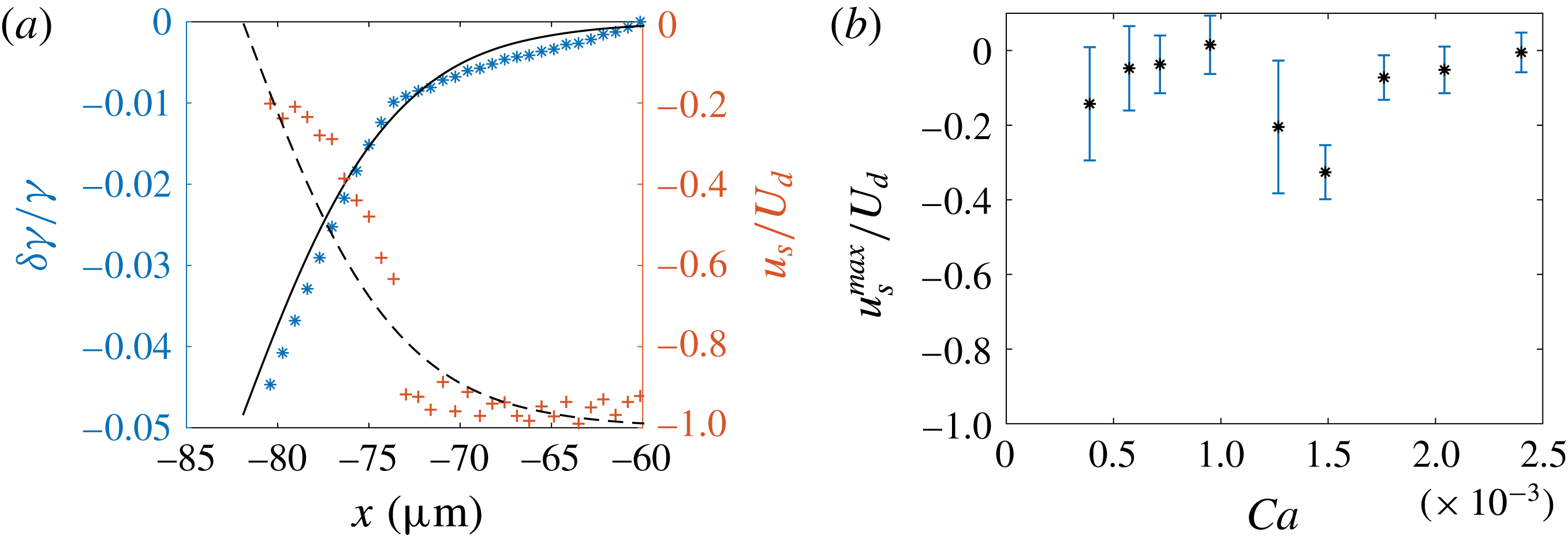
It is important to note that a significant difference between our geometry and the rising bubble in three dimensions studied in Cuenot et al. (Reference Cuenot, Magnaudet and Spennato1997) is that the Marangoni effect, i.e. the surface tension gradient, has a direct signature on the film thickness. We thus determine the surface tension profile from the experimental value of the thickness, and we compare them to our theoretical predictions. The interface velocity field is extracted from (4.10) and the surface tension is then obtained from (4.11), which can be integrated to
 $$\begin{eqnarray}\unicode[STIX]{x1D6FF}\unicode[STIX]{x1D6FE}(x)=\unicode[STIX]{x1D702}_{o}\int _{x_{min}}^{x}\frac{u_{s}(x^{\prime })+U_{d}}{h(x^{\prime },0)}\,\text{d}x^{\prime },\end{eqnarray}$$
with
 $x_{min}=-60~\unicode[STIX]{x03BC}\text{m}$
an arbitrary value far from the rear meniscus, where the surface tension is the reference one.
(a) Surface tension (
 $\ast$
) and interfacial velocity (
 $+$
) in the thickening region, relative to their values in the flat film. Data points are obtained by applying (4.10) and (4.17) to the experimental thickness profile for
 $Ca=1.3\times 10^{-3}$
(figure 6
b). Solid and dashed lines correspond, respectively, to the interfacial tension and velocity deduced from (4.16) with
 $Ma=1.6$
. (b) Variation of the maximum interfacial velocity at the bump relative to that of the droplet, as a function of
 $Ca$
.
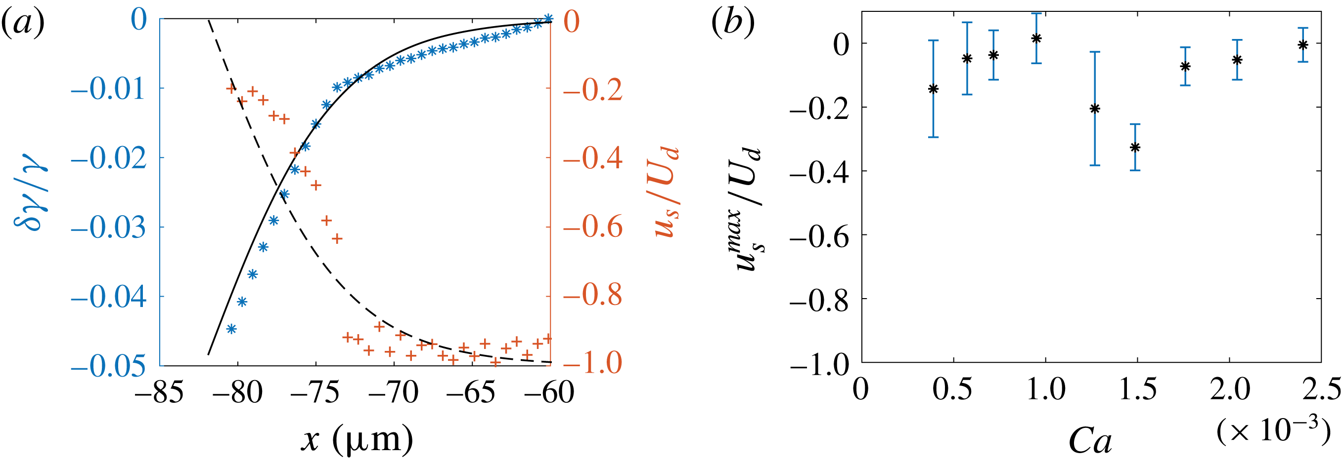
Equation (4.10) gives access to the interfacial velocity profile in the thickening region, shown in figure 8(a). It varies from
 $-U_{d}$
in the flat film to a maximal value at the bump,
 $u_{s}^{max}$
, in the range
 $[-0.3,-0.1]U_{d}$
; see figure 8(b). The relative interfacial tension variation
 $\unicode[STIX]{x1D6FF}\unicode[STIX]{x1D6FE}(x)/\unicode[STIX]{x1D6FE}$
is plotted in figure 8(a). The surface tension decreases from
 $\unicode[STIX]{x1D6FE}=15~\text{mN}~\text{m}^{-1}$
in the flat film (the reference value at equilibrium) to a smaller value
 $\unicode[STIX]{x1D6FE}_{min}$
at the top of the bump. The value
 $\unicode[STIX]{x0394}\unicode[STIX]{x1D6FE}=\unicode[STIX]{x1D6FE}_{min}-\unicode[STIX]{x1D6FE}$
is constant over our range of capillary numbers within the precision of our error bars, and of the order of
 $\unicode[STIX]{x0394}\unicode[STIX]{x1D6FE}\sim -5\times 10^{-4}~\text{N}~\text{m}^{-1}$
, which corresponds to a
 ${\sim}3\,\%$
decrease. These predictions are obtained using (4.10) and (4.11), which do not rely on any assumption about surfactant transport. They are valid whatever the interfacial rheology, as long as the Laplace pressure variations are negligible. Remarkably, both the surface tension and surface velocity variations directly deduced from
 $h$
are consistent with the full model, with
 $Ma=1.6$
– see lines in figure 8(a).
We now turn to the oscillating region, closer to the rear meniscus, where both the Laplace pressure effect and the presence of surfactant at the interface contribute. We propose a semi-empirical model to predict the film profile in this domain. In light of the previous analysis, we assume an incompressible interface of uniform velocity
 $u_{s}^{max}$
, measured above. Equation (4.2) then becomes
 $$\begin{eqnarray}-\!\unicode[STIX]{x1D6FE}\frac{\unicode[STIX]{x2202}^{3}h}{\unicode[STIX]{x2202}x^{3}}=\frac{6\unicode[STIX]{x1D702}_{o}}{h^{3}}[u_{s}^{max}-U_{d}][h-h_{\infty }^{\ast }],\end{eqnarray}$$
with
 $u_{s}^{max}=U_{d}(1-2h_{\infty }/h_{max})$
. The curvature at small
 $x$
is
 $1/H_{0}$
and the film thickness
 $h_{\infty }^{\ast }$
at large
 $x$
is fitted so that the maximum height
 $h_{max}$
is recovered by the model, i.e.
 $h_{\infty }^{\ast }=h_{max}/1.064$
. This numerical prediction is now in very good agreement with the experimental back oscillation (see solid lines in figure 6
d–f), thus validating that the interface velocity does not vary much once it reaches values as big as
 $u_{s}^{max}$
.
4.4 Conclusion
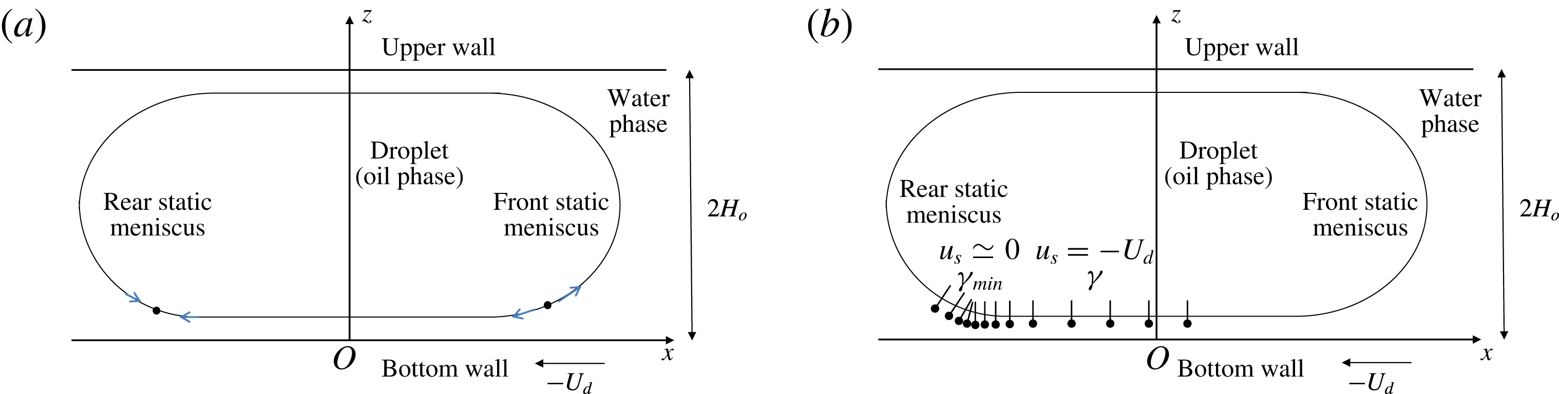
These results are consistent with the accumulation of surfactants at the rear of the droplet, transported from the drop front by convection: the interface flows at the velocity
 $-U_{d}$
in the film, and thus brings surfactant into the rear region. If axial diffusion is not fast enough, surfactants accumulate and reduce the surface tension. This induces a Marangoni stress, which, in turn, reduces the amplitude of the backwards interface velocity. Figure 9 provides a schematic representation of the mechanisms at play. The resulting Marangoni stress imposes a constant interfacial velocity in the oscillating region. The thickening region corresponds to a compression zone in the thin film, where the interfacial velocity rapidly increases from a value close to the wall velocity in the flat film, to a value close to the droplet velocity at the rear. The signature of this transition is a sudden thickening of the film.
Schematic side views of the droplet. (a) Bretherton’s classical model predicts two stagnation points: a divergent one in the front dynamical meniscus, and a convergent one in the rear dynamical meniscus. (b) Representation of a surfactant concentration field at the interface, consistent with our measurements for the interfacial velocity.
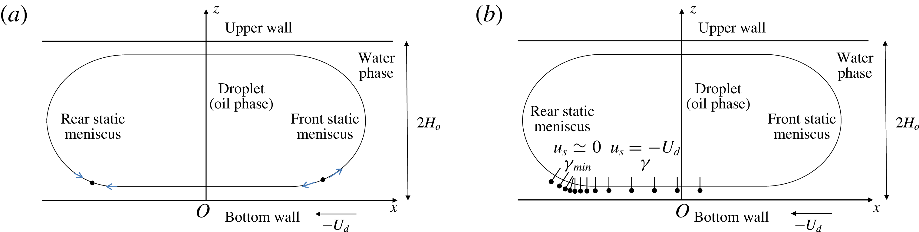
In a nutshell, the lubrication film must be split into three regions in terms of boundary conditions: (1) the front meniscus and flat film, with a stress-free interface; (2) the oscillating region at the rear meniscus, with an incompressible interface of velocity
 $u_{s}^{max}$
; and (3) a transition zone, or thickening region, between the first two.
5 Transverse film profiles
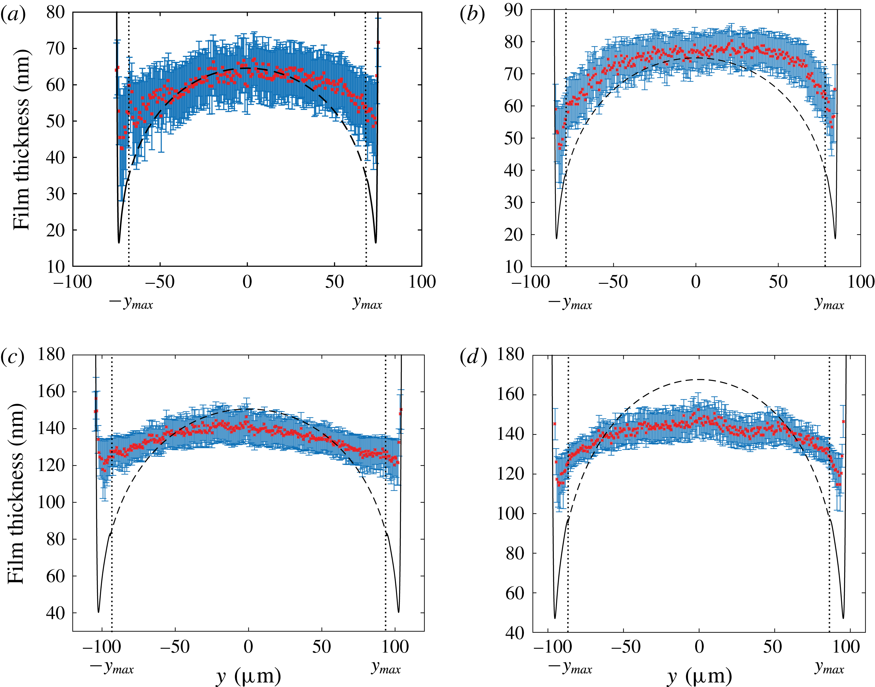
The transverse variation of the film thickness
 $h(0,y)$
as a function of
 $y$
is shown in figure 10. By definition,
 $h_{\infty }(y)=h(0,y)$
for
 $|y|<y_{max}$
. In this domain,
 $h_{\infty }(y)$
is maximal for
 $y=0$
and slowly decreases as
 $|y|$
increases. Then for
 $|y|>y_{max}$
, the thickness decreases with a steeper slope before increasing sharply close to the lateral meniscus, creating what we refer to as lateral ravines.
5.1 Central region and front meniscus
Burgess & Foster (Reference Burgess and Foster1990) showed that Bretherton’s 2D approach remains valid close to the front of the droplet if the capillary number is defined using the projection of the droplet’s velocity along the normal to the film contour
 $\boldsymbol{e}_{\unicode[STIX]{x1D70C}}$
. This can be understood qualitatively at the scale of the dynamical meniscus, in the local frame
 $(\boldsymbol{e}_{\unicode[STIX]{x1D70C}},\boldsymbol{e}_{\unicode[STIX]{x1D703}},\boldsymbol{e}_{z})$
. In the plane
 $(\boldsymbol{e}_{\unicode[STIX]{x1D746}},\boldsymbol{e}_{\boldsymbol{z}})$
chosen at an arbitrary angle
 $\unicode[STIX]{x1D703}^{fr}\ll \unicode[STIX]{x03C0}/2$
(figure 3), Bretherton’s problem is recovered: the Laplace pressure is governed by the curvature
 $1/H_{o}$
of a meniscus quasi-invariant in the
 $\boldsymbol{e}_{\unicode[STIX]{x1D703}}$
direction, the viscous forces are governed by the wall velocity
 $-U_{d}\cos (\unicode[STIX]{x1D703}^{fr})$
, and the tangential wall velocity
 $U_{d}\sin (\unicode[STIX]{x1D703}^{fr})$
has no influence on the profile. Since the thickness of the lubrication film deposited behind the front dynamical meniscus is determined by the balance of the viscous and Laplace pressure contributions, it is expected to decrease with increasing
 $\unicode[STIX]{x1D703}^{fr}$
.


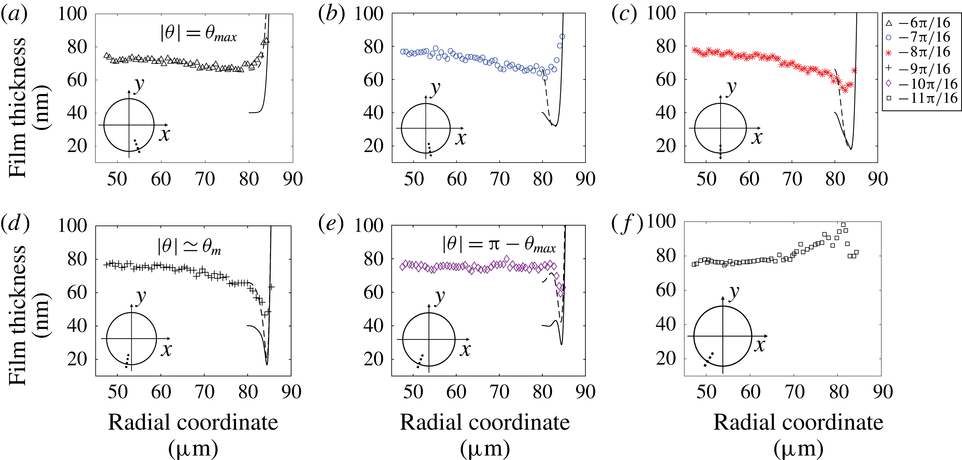
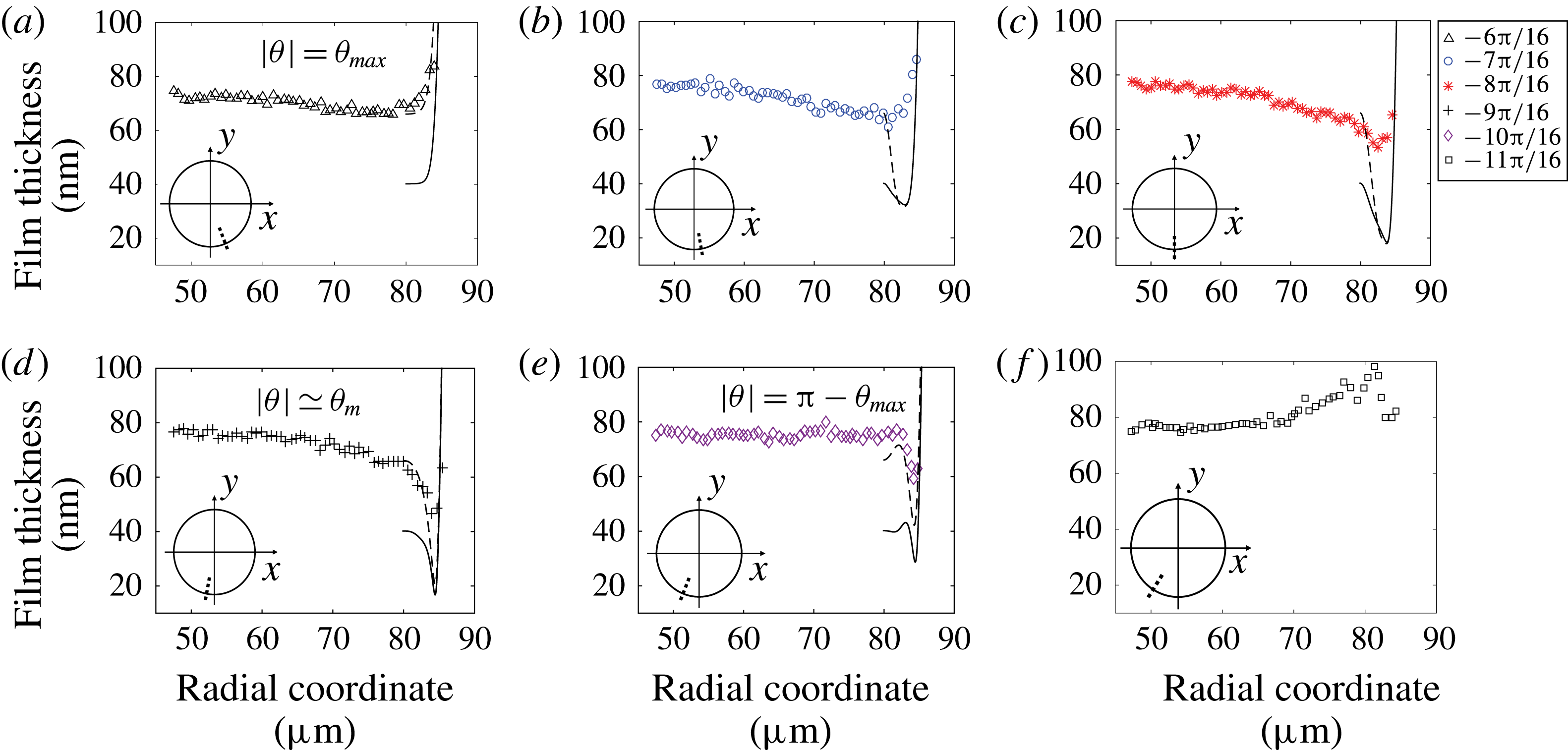
Radial profiles for (a)
 $\unicode[STIX]{x1D703}=-6\unicode[STIX]{x03C0}/16\simeq \unicode[STIX]{x1D703}_{max}$
, (b)
 $\unicode[STIX]{x1D703}=-7\unicode[STIX]{x03C0}/16$
, (c)
 $\unicode[STIX]{x1D703}=-8\unicode[STIX]{x03C0}/16$
, (d)
 $\unicode[STIX]{x1D703}=-9\unicode[STIX]{x03C0}/16$
, (e)
 $\unicode[STIX]{x1D703}=-10\unicode[STIX]{x03C0}/16$
and (f)
 $\unicode[STIX]{x1D703}=-11\unicode[STIX]{x03C0}/16$
for
 $Ca=7.2\times 10^{-4}$
. Solid line: solution of (5.5) with the numerical profile
 $h^{num}(\unicode[STIX]{x1D70C},\unicode[STIX]{x1D703}_{max})$
as initial condition, i.e. the solution of (5.3) for
 $\unicode[STIX]{x1D703}=\unicode[STIX]{x1D703}_{max}=\unicode[STIX]{x03C0}/2-\unicode[STIX]{x1D6FF}_{\unicode[STIX]{x1D703}}^{\prime }\unicode[STIX]{x1D719}_{max}^{\prime }$
. Dashed line: solution of (5.5) using the experimental profile
 $h^{exp}(\unicode[STIX]{x1D70C},\unicode[STIX]{x1D703}_{max})$
as an initial condition. Insets: the dotted line indicates the location of the radial profile for each angle value.
Then, far enough from the front dynamical meniscus along
 $\boldsymbol{e}_{\unicode[STIX]{x1D70C}}$
, the pressure gradients scale as
 $\unicode[STIX]{x1D735}P^{film}\sim \unicode[STIX]{x1D6FE}h_{\infty }/R^{3}$
. This pressure gradient induces velocities of order
 $\unicode[STIX]{x1D735}P^{film}h^{2}/\unicode[STIX]{x1D702}_{o}\sim 10^{-8}~\text{m}~\text{s}^{-1}$
, which are negligible compared to our droplet velocities. Once formed in the front meniscus domain, the thin film stays at rest on the wall in the central region until it reaches the rear meniscus domain. The film thickness
 $h^{BF,c}(y)$
in the central region is thus determined by the velocity normal to the droplet’s contour at the same value of
 $y$
,
 $-U_{d}\cos (\unicode[STIX]{x1D703}^{fr})$
, and does not depend on
 $x$
. This leads to the following prediction for the central film (Burgess & Foster Reference Burgess and Foster1990):
 $$\begin{eqnarray}h^{BF,c}(y)=1.337H_{o}[Ca\cos (\unicode[STIX]{x1D703}^{fr})]^{2/3}=1.337H_{o}Ca^{2/3}\left[1-\frac{y^{2}}{R^{2}}\right]^{1/3}.\end{eqnarray}$$
This corresponds to a weighted Bretherton model, based on the local normal velocity in the front meniscus domain. A similar approach, using the normal velocity to introduce a modified capillary number, was adopted in Nagel (Reference Nagel2014) to derive the viscous friction in the dynamical meniscus of a Hele-Shaw droplet. The transverse variation of
 $h_{\infty }(y)$
is compared to
 $h^{BF,c}(y)$
in figure 10, for
 $|y|<y_{max}$
. We find that the vault shape of the experimental profile is qualitatively recovered by the model, but the decrease on the sides is overestimated. The disjoining pressure cannot be responsible for that thickening. Indeed, as stated in § 2.2, the main contribution setting a film thickness above 40 nm is clearly attributed to hydrodynamics while van der Waals dispersion contribution lies within the error bar.
5.2 Lateral region
At
 $y=y_{max}$
the front meniscus domain ends without sharp transition (see § 3). In the lateral region, the polar coordinates are more convenient, and we consider below
 $h(\unicode[STIX]{x1D70C},\unicode[STIX]{x1D703})$
. In this region, for a given
 $\unicode[STIX]{x1D703}$
,
 $h(\unicode[STIX]{x1D70C},\unicode[STIX]{x1D703})$
first decreases before increasing, i.e. a pinch develops; see the radial profiles plotted in figure 11. We define the film thickness at the pinch
 $h_{p}(\unicode[STIX]{x1D703})$
as the minimum of
 $h(\unicode[STIX]{x1D70C},\unicode[STIX]{x1D703})$
for a given
 $\unicode[STIX]{x1D703}$
in the lateral domain. The variation of
 $h_{p}(\unicode[STIX]{x1D703})$
with
 $\unicode[STIX]{x1D703}$
is shown in figure 13(c):
 $h_{p}(\unicode[STIX]{x1D703})$
decreases down to a minimal value
 $h_{min}$
, for
 $\unicode[STIX]{x1D703}_{m}$
slightly larger than
 $\unicode[STIX]{x03C0}/2$
, then increases under the influence of the rear meniscus. For
 $|\unicode[STIX]{x1D703}|$
larger than a critical angle
 $\unicode[STIX]{x1D703}_{b}\in [\unicode[STIX]{x1D703}_{m};\unicode[STIX]{x03C0}-\unicode[STIX]{x1D703}_{max}]$
, there is a bump preceding the pinch (see figure 11
e,f).
5.2.1 Hydrodynamical approach
To describe formally the lateral meniscus, a weighted 2D Bretherton model based on the normal velocity is no longer physical, since the meniscus is no longer perpendicular to the flow, and would lead to a null film thickness for
 $\unicode[STIX]{x1D703}=\unicode[STIX]{x03C0}/2$
. In this region, the orthoradial viscous entrainment, stemming from the orthoradial wall velocity
 $U_{d}\sin (\unicode[STIX]{x1D703})$
, has to be considered. To account for this truly 3D process, the lubrication equations established by Burgess & Foster (Reference Burgess and Foster1990) are adapted to our geometry and solved numerically. This model relies on the same approximations as previously, except for the assumption of transverse translational invariance. The Stokes equation in the lubrication approximation,
 $\unicode[STIX]{x1D6FB}^{2D}p=\unicode[STIX]{x1D702}_{o}\unicode[STIX]{x2202}^{2}\boldsymbol{u}/\unicode[STIX]{x2202}z^{2}$
, is written in cylindrical coordinates and integrated three times with respect to
 $z$
to get the flow through the film thickness
 $h$
. The boundary conditions are
 $\boldsymbol{u}(0)=-U_{d}\boldsymbol{e}_{x}$
and
 $\unicode[STIX]{x2202}\boldsymbol{u}/\unicode[STIX]{x2202}z(h)=0$
. Applying the continuity equation to the flow yields
 $$\begin{eqnarray}U_{d}\cos \unicode[STIX]{x1D703}\,\frac{\unicode[STIX]{x2202}h}{\unicode[STIX]{x2202}\unicode[STIX]{x1D70C}}-\frac{U_{d}\sin \unicode[STIX]{x1D703}}{\unicode[STIX]{x1D70C}}\,\frac{\unicode[STIX]{x2202}h}{\unicode[STIX]{x2202}\unicode[STIX]{x1D703}}-\frac{\unicode[STIX]{x2202}}{\unicode[STIX]{x2202}\unicode[STIX]{x1D70C}}\left[\frac{\unicode[STIX]{x1D6FE}}{3\unicode[STIX]{x1D702}_{o}}\,\frac{\unicode[STIX]{x2202}^{3}h}{\unicode[STIX]{x2202}\unicode[STIX]{x1D70C}^{3}}h^{3}\right]=0\end{eqnarray}$$
(see details in appendix B).
The second term of (5.2) is negligible for angle
 $\unicode[STIX]{x1D703}$
up to
 $\unicode[STIX]{x1D703}=\unicode[STIX]{x1D703}_{max}$
since the orthoradial variation
 $(1/\unicode[STIX]{x1D70C})(\unicode[STIX]{x2202}h/\unicode[STIX]{x2202}\unicode[STIX]{x1D703})$
of
 $h$
is much smaller than the radial variation
 $\unicode[STIX]{x2202}h/\unicode[STIX]{x2202}\unicode[STIX]{x1D70C}$
of
 $h$
for
 $H_{0}\ll R$
. In this condition, the second term can be neglected in (5.2), for
 $\unicode[STIX]{x1D703}<\unicode[STIX]{x1D703}_{max}$
, so that Bretherton’s equation (4.4) is recovered using the local normal velocity
 $U_{d}\cos \unicode[STIX]{x1D703}$
:
 $$\begin{eqnarray}U_{d}\cos \unicode[STIX]{x1D703}\,(h-h_{\infty })=\frac{\unicode[STIX]{x1D6FE}}{3\unicode[STIX]{x1D702}_{o}}\frac{\unicode[STIX]{x2202}^{3}h}{\unicode[STIX]{x2202}\unicode[STIX]{x1D70C}^{3}}h^{3}.\end{eqnarray}$$
As discussed earlier, solving this equation leads to the solution (5.1).
On the lateral side of the droplet, however, the orthoradial component of the viscous driving has to be considered and all three terms of (5.2) must be taken into account. To build a master equation, ensuring that the first two terms in (5.2) are of the same order of magnitude as long as the rescaled angle is of order 1, Burgess & Foster (Reference Burgess and Foster1990) introduce the following rescalings:
 $$\begin{eqnarray}\unicode[STIX]{x1D70C}=R+H_{o}\unicode[STIX]{x1D6FF}_{r}r^{\prime },\quad z=H_{o}\unicode[STIX]{x1D6FF}_{z}z^{\prime },\quad h=H_{o}\unicode[STIX]{x1D6FF}_{z}h^{\prime },\quad \unicode[STIX]{x1D703}-\frac{\unicode[STIX]{x03C0}}{2}=\unicode[STIX]{x1D719}=\unicode[STIX]{x1D6FF}_{\unicode[STIX]{x1D703}}\unicode[STIX]{x1D719}^{\prime },\end{eqnarray}$$
where
 $\unicode[STIX]{x1D6FF}_{r}=(\unicode[STIX]{x1D716}^{1/2}Ca)^{2/5}$
,
 $\unicode[STIX]{x1D6FF}_{z}=(\unicode[STIX]{x1D716}^{1/2}Ca)^{4/5}$
and
 $\unicode[STIX]{x1D6FF}_{\unicode[STIX]{x1D703}}=\unicode[STIX]{x1D716}^{1/2}(\unicode[STIX]{x1D716}^{1/2}Ca)^{1/5}$
. These quantities involve
 $\unicode[STIX]{x1D716}=H_{0}/R$
and the capillary number
 $Ca$
, under the assumption
 $Ca\ll \unicode[STIX]{x1D716}\ll 1$
. With
 $Ca=7.2\times 10^{-4}$
and
 $\unicode[STIX]{x1D716}=8\times 10^{-2}$
, we get
 $\unicode[STIX]{x1D6FF}_{r}=0.03$
,
 $\unicode[STIX]{x1D6FF}_{z}=0.001$
and
 $\unicode[STIX]{x1D6FF}_{\unicode[STIX]{x1D703}}=0.05~\text{rad}=3^{\circ }$
. Using these non-dimensional variables and a first-order expansion of the sine and cosine terms around
 $\unicode[STIX]{x03C0}/2$
, (5.2) becomes
 $$\begin{eqnarray}({\textstyle \frac{1}{3}}h_{r^{\prime }r^{\prime }r^{\prime }}^{\prime }h^{^{\prime }3}+\unicode[STIX]{x1D719}^{\prime }h^{\prime })_{r^{\prime }}=-h_{\unicode[STIX]{x1D719}^{\prime }}^{\prime }.\end{eqnarray}$$
5.2.2 Analogy with marginal pinching in soap films
To put this last equation in a different light, it is worth noting that, by taking out the term for a radial viscous supply of liquid (
 $(\unicode[STIX]{x1D719}^{\prime }h^{\prime })_{r^{\prime }}$
, negligible for
 $\unicode[STIX]{x1D703}\sim \unicode[STIX]{x03C0}/2$
) and replacing
 $\unicode[STIX]{x1D719}^{\prime }$
by the time
 $t$
, we recover the equation describing the drainage of a soap film (Aradian, Raphael & De Gennes Reference Aradian, Raphael and De Gennes2001). In other words, in this region the lubrication film can be pictured as a soap film being drained along
 $\unicode[STIX]{x1D703}$
, rather than over time. The capillary suction by the lateral meniscus is responsible for the appearance of the pinch for
 $\unicode[STIX]{x1D703}>\unicode[STIX]{x1D703}_{max}$
on both sides of the droplet (see figure 11).
Analogy with a soap film deposited along
 $\unicode[STIX]{x1D703}$
rather than over time. (a) A film of thickness
 $h_{\infty }(\unicode[STIX]{x1D719}_{max})=1.337H_{o}Ca^{2/3}(\unicode[STIX]{x1D719}_{max})^{2/3}$
is deposited at
 $(R,-\unicode[STIX]{x1D719}_{max})=(R,-(\unicode[STIX]{x03C0}/2-\unicode[STIX]{x1D703}_{max}))$
and (b) thins until the influence of the rear meniscus is felt.

This process is quantified by Aradian et al. (Reference Aradian, Raphael and De Gennes2001) in a 2D geometry, much simpler than the 3D droplet investigated by Burgess & Foster (Reference Burgess and Foster1990) and the present work. However, we can establish that the scalings obtained for the pinch thickness and width are identical in both cases. In Aradian et al. (Reference Aradian, Raphael and De Gennes2001), a foam film is put into contact with a meniscus at time
 $t=0$
. The film is pinched, with a minimal thickness
 $H^{m}$
and a pinch width
 $W$
evolving over time. They assume a no-slip condition at the air–liquid interfaces, so that the problem is equivalent to a film deposited on a solid wall, with a stress-free condition at the air–liquid interface, and can be directly translated to our case.
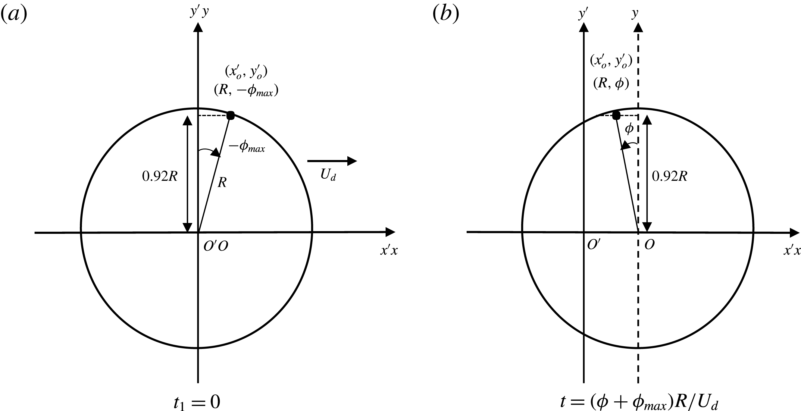
We look at the droplet motion in the laboratory frame of reference,
 $(O^{\prime },x^{\prime },y^{\prime },z^{\prime })$
; the geometrical parameters used are defined in figure 12. A thin film is produced at a position
 $(x^{\prime },y^{\prime })$
when the front of the droplet passes that point, at time denoted
 $t_{1}$
. The rear meniscus reaches this point
 $(x^{\prime },y^{\prime })$
at the time denoted
 $t_{2}$
. If
 $y^{\prime }\ll R$
, i.e. close to the
 $x$
axis, the fluid velocity is negligible in the central film (see § 5.1) and the thin film is thus at rest on the wall between
 $t_{1}$
and
 $t_{2}$
. However, close to the lateral meniscus, this assumption fails. The lateral capillary suction (in the
 $y^{\prime }$
direction) induces a film thinning lasting between times
 $t_{1}$
and
 $t_{2}$
and the formation of the pinch.
To compare our study with Aradian’s one, we consider the film deposited at the point
 $(x_{0}^{\prime },y_{0}^{\prime })$
, with
 $y_{0}^{\prime }=y_{max}$
. It has the polar coordinates (
 $\unicode[STIX]{x1D70C}=R;\unicode[STIX]{x1D719}=-\unicode[STIX]{x1D719}_{max}=-(\unicode[STIX]{x03C0}/2-\unicode[STIX]{x1D703}_{max})$
) at the time
 $t_{1}$
(with the laboratory and drop frames at the same position at time
 $t_{1}$
). For the sake of convenience, we choose
 $t_{1}=0$
. The thickness of the deposited thin film is
 $h_{\infty }(\unicode[STIX]{x1D719}_{max})=1.337H_{o}Ca^{2/3}(\unicode[STIX]{x1D719}_{max})^{2/3}$
(at first order in
 $\unicode[STIX]{x1D719}_{max}$
). At a later time
 $t$
, the polar coordinates are (
 $\unicode[STIX]{x1D70C}=R;\unicode[STIX]{x1D719}=-\unicode[STIX]{x1D719}_{max}+U_{d}t/R$
) (see figure 12). So the age of the film since the beginning of the pinching process is simply
 $t=(\unicode[STIX]{x1D719}+\unicode[STIX]{x1D719}_{max})R/U_{d}$
.
The scaling laws at long times for the pinch profile give us (Aradian et al. Reference Aradian, Raphael and De Gennes2001):
 $$\begin{eqnarray}\displaystyle \left.\begin{array}{@{}c@{}}\displaystyle W\sim H_{o}\left(\frac{\unicode[STIX]{x1D702}_{o}h_{\infty }(\unicode[STIX]{x1D719}_{max})}{\unicode[STIX]{x1D6FE}}\right)^{1/4}(t)^{-1/4},\\ \displaystyle H^{m}\sim H_{o}\left(\frac{\unicode[STIX]{x1D702}_{o}h_{\infty }(\unicode[STIX]{x1D719}_{max})}{\unicode[STIX]{x1D6FE}}\right)^{1/2}(t)^{-1/2}.\end{array}\right\} & & \displaystyle\end{eqnarray}$$
In these equations, the theoretical value of
 $\unicode[STIX]{x1D719}_{max}$
remains to be determined. It corresponds to the point where the film thickness gradient, projected along
 $x$
, is no longer dominated by the radial gradient (Burgess & Foster Reference Burgess and Foster1990). In the lateral region, at the first order in
 $\unicode[STIX]{x1D719}$
,
 $\unicode[STIX]{x2202}h/\unicode[STIX]{x2202}x=-(1/R)(\unicode[STIX]{x2202}h/\unicode[STIX]{x2202}\unicode[STIX]{x1D719})-\unicode[STIX]{x1D719}(\unicode[STIX]{x2202}h/\unicode[STIX]{x2202}\unicode[STIX]{x1D70C})$
. Equating the two contributions at
 $\unicode[STIX]{x1D719}=\unicode[STIX]{x1D719}_{max}$
, and using
 $\unicode[STIX]{x2202}/\unicode[STIX]{x2202}\unicode[STIX]{x1D719}\sim 1/\unicode[STIX]{x1D719}_{max}$
and
 $\unicode[STIX]{x2202}/\unicode[STIX]{x2202}\unicode[STIX]{x1D70C}\sim 1/W$
, we get
 $\unicode[STIX]{x1D719}_{max}=(W/R)^{1/2}$
. Inserting that in
 $h_{\infty }(\unicode[STIX]{x1D719}_{max})$
and solving the system (5.6) yields
 $$\begin{eqnarray}\displaystyle \left.\begin{array}{@{}c@{}}\displaystyle W\sim H_{o}\left(\frac{H_{o}}{R}\right)^{1/5}Ca^{2/5}\left(1+\frac{\unicode[STIX]{x1D719}}{\unicode[STIX]{x1D719}_{max}}\right)^{-1/4},\\ \displaystyle H^{m}\sim H_{o}\left(\frac{H_{o}}{R}\right)^{2/5}Ca^{4/5}\left(1+\frac{\unicode[STIX]{x1D719}}{\unicode[STIX]{x1D719}_{max}}\right)^{-1/2},\\ \displaystyle \unicode[STIX]{x1D719}_{max}\sim \left(\frac{H_{o}}{R}\right)^{3/5}Ca^{1/5}.\end{array}\right\} & & \displaystyle\end{eqnarray}$$
This is the same scaling as the one established by Burgess & Foster (Reference Burgess and Foster1990).
As a last remark, the interface profile at given time (or angle in our situation) is related to two different length scales in Aradian et al. (Reference Aradian, Raphael and De Gennes2001): the radius of curvature in the vicinity of the pinch, and the distance between the minimal thickness and the unperturbed flat film. The first one scales as
 $W$
, which decreases with
 $\unicode[STIX]{x1D719}$
, whereas the second scales as
 $\unicode[STIX]{x1D706}\sim H_{o}Ca^{3/5}(H_{o}/R)^{1/5}(1+\unicode[STIX]{x1D719}/\unicode[STIX]{x1D719}_{max})^{1/4}$
, which increases with
 $\unicode[STIX]{x1D719}$
. The presence of two different length scales to characterize the interface profile in the radial direction means that, contrary to the front dynamical meniscus, the profiles are not self-similar in the lateral region.
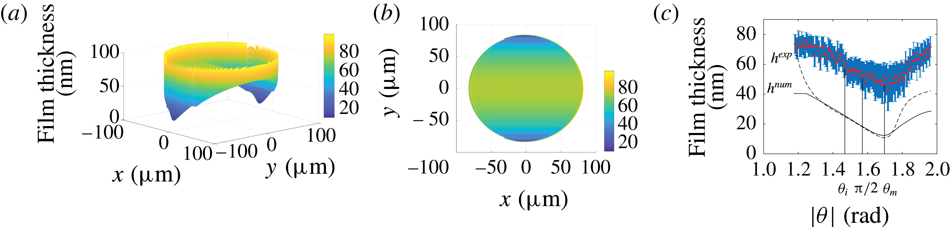
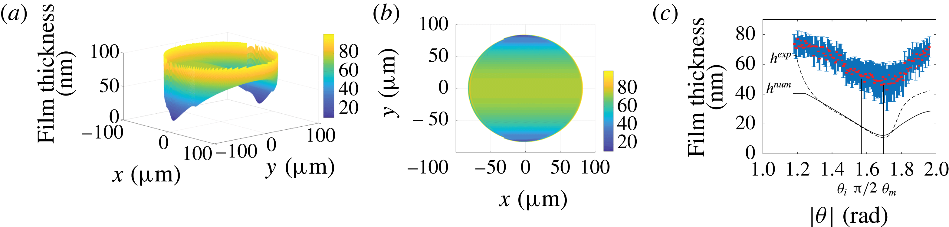
(a) Numerical topography obtained by joining the profiles calculated in the different dynamical menisci with the central domain for
 $Ca=7.2\times 10^{-4}$
. (b) Colour map of the lubrication film thickness for
 $Ca=7.2\times 10^{-4}$
. (c) Minimum film thickness across the pinch
 $h_{p}(\unicode[STIX]{x1D703})$
as a function of
 $\unicode[STIX]{x1D703}$
for
 $|\unicode[STIX]{x1D703}|\in [\unicode[STIX]{x1D703}_{max};\unicode[STIX]{x03C0}-\unicode[STIX]{x1D703}_{max}]$
. The inflection point occurs for
 $\unicode[STIX]{x1D703}_{i}=1.47~\text{rad}$
and the minimal thickness
 $h_{min}$
is reached for
 $\unicode[STIX]{x1D703}_{m}=1.72~\text{rad}$
. Solid line: solution of (5.5) using the solution of (5.3) for
 $\unicode[STIX]{x1D703}=\unicode[STIX]{x1D703}_{max}=\unicode[STIX]{x03C0}/2-\unicode[STIX]{x1D6FF}_{\unicode[STIX]{x1D703}}^{\prime }\unicode[STIX]{x1D719}_{max}^{\prime }$
,
 $h^{num}(\unicode[STIX]{x1D70C},\unicode[STIX]{x1D703}_{max})$
, as an initial condition for the numerical calculation. Dashed line: solution of (5.5) using the experimental profile for
 $\unicode[STIX]{x1D703}=\unicode[STIX]{x1D703}_{max}$
,
 $h^{exp}(\unicode[STIX]{x1D70C},\unicode[STIX]{x1D703}_{max})$
, as an initial condition.
5.2.3 Results and discussion
To compare that theoretical approach to our experimental data, we establish numerical profiles by solving (5.5) for
 $-\unicode[STIX]{x1D719}_{max}^{\prime }\leqslant \unicode[STIX]{x1D719}^{\prime }\leqslant \unicode[STIX]{x1D719}_{max}^{\prime }$
with
 $\unicode[STIX]{x1D719}_{max}^{\prime }=7.5$
and
 $-18\leqslant r^{\prime }\leqslant 26$
. This corresponds, in physical units, to the parameter range
 $[\unicode[STIX]{x1D703}_{max};\unicode[STIX]{x03C0}-\unicode[STIX]{x1D703}_{max}]$
and
 $[\unicode[STIX]{x1D70C}_{min}=79~\unicode[STIX]{x03BC}\text{m};\unicode[STIX]{x1D70C}_{max}=90~\unicode[STIX]{x03BC}\text{m}]$
. A profile
 $h^{\prime }(r^{\prime },-\unicode[STIX]{x1D719}_{max}^{\prime })$
is chosen as an initial condition and the profiles
 $h^{\prime }(r^{\prime },\unicode[STIX]{x1D719}^{\prime })$
for larger angles are obtained using a Crank–Nicolson scheme. The boundary conditions are a constant curvature in the meniscus,
 $\text{d}^{2}h/\text{d}r^{2}(\unicode[STIX]{x1D70C}_{max})=1/H_{o}$
, and a connection to a flat film of constant thickness,
 $h(\unicode[STIX]{x1D70C}_{min},\unicode[STIX]{x1D703})=h(\unicode[STIX]{x1D70C}_{min},\unicode[STIX]{x1D703}_{max})$
. The simulations have been performed using either the numerical profile from (5.3),
 $h^{num}(\unicode[STIX]{x1D70C},\unicode[STIX]{x1D703}_{max})$
, or the experimental profile
 $h^{exp}(\unicode[STIX]{x1D70C},\unicode[STIX]{x1D703}_{max})$
for the initial condition at
 $\unicode[STIX]{x1D719}^{\prime }=-\unicode[STIX]{x1D719}_{max}^{\prime }$
. An example of the numerical topography of the film obtained by joining the calculated profiles in the different dynamical menisci with the central domain is shown in figure 13(a,b), while the solid line and the dashed line in figure 13(c) are the solutions of (5.5) computed, respectively, from
 $h^{num}(\unicode[STIX]{x1D70C},\unicode[STIX]{x1D703}_{max})$
and
 $h^{exp}(\unicode[STIX]{x1D70C},\unicode[STIX]{x1D703}_{max})$
.
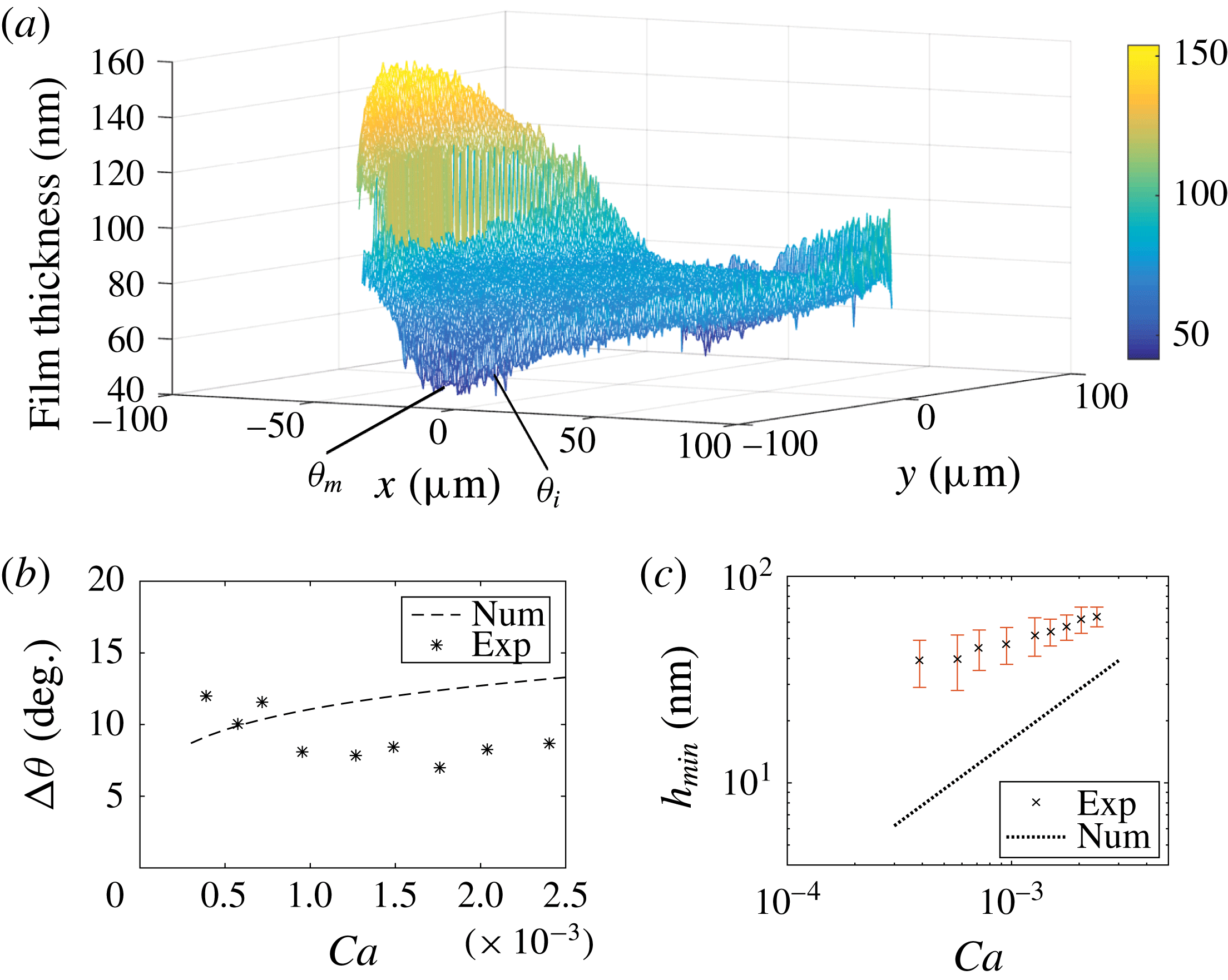
(a) Experimental topography for
 $Ca=7.2\times 10^{-4}$
. (b) Angular extent of the lateral meniscus as a function of
 $Ca$
. The dashed line is
 $\unicode[STIX]{x0394}\unicode[STIX]{x1D703}$
given by the numerical calculation. (c) Minimal film thickness in the lateral region,
 $h_{min}$
, as a function of
 $Ca$
. The dotted line is
 $h_{min}$
obtained from the numerical calculation.

Several qualitative features are well recovered by the simulations. As expected, a pinch develops (see figure 11) as the film thickness decreases slowly from the initial condition before increasing sharply near the rear meniscus (see figure 13
c). Its characteristic width in the
 $\boldsymbol{e}_{\unicode[STIX]{x1D70C}}$
direction is in good agreement with the experimental observations (see figure 11). In agreement with (5.7),
 $W$
decreases with
 $\unicode[STIX]{x1D719}$
for
 $\unicode[STIX]{x1D719}\in [-\unicode[STIX]{x1D719}_{max};\unicode[STIX]{x1D719}_{m}]$
(
 $\unicode[STIX]{x1D719}_{m}=\unicode[STIX]{x1D703}_{m}-\unicode[STIX]{x03C0}/2$
); however, our image resolution does not allow us to measure a power-law exponent for its variation with
 $\unicode[STIX]{x1D719}$
or
 $Ca$
. The angles
 $\unicode[STIX]{x1D703}_{m}$
, corresponding to the smallest pinch thickness, and
 $\unicode[STIX]{x1D703}_{b}$
, at which the bump appears, are both predicted quantitatively (see figure 11
d,e). The angle
 $\unicode[STIX]{x1D703}_{i}$
, shown in figures 13(c) and 14(a), is that at which the curvature inversion occurs and is used to measure the ravines’ angular extension. The angular extent of the pinch,
 $\unicode[STIX]{x0394}\unicode[STIX]{x1D703}=\unicode[STIX]{x1D703}_{m}-\unicode[STIX]{x1D703}_{i}$
, is measured from
 $h_{p}(\unicode[STIX]{x1D703})$
, and its variation with
 $Ca$
is shown in figure 14(b), for both experimental and numerical datasets. The correct order of magnitude is recovered, though we cannot draw conclusions on the trend in
 $Ca$
.
In contrast, the film thickness at the pinch is strongly underestimated by the model, for every capillary number and independently of the initial conditions. The minimum film thickness in the lateral meniscus,
 $h_{min}$
, does not seem to follow the predicted scaling
 $\propto Ca^{4/5}$
(figure 14
c). As for
 $h_{p}(\unicode[STIX]{x1D703})$
, or equivalently
 $H^{m}$
, the angular range
 $|\unicode[STIX]{x1D703}|\in [\unicode[STIX]{x1D703}_{i},\unicode[STIX]{x1D703}_{m}]$
over which the scaling from (5.7) can be compared to the experimental profile (figure 13
c), and predicts a decrease with
 $\unicode[STIX]{x1D703}$
, is too small to allow us to measure a power-law exponent. Then, for
 $|\unicode[STIX]{x1D703}|>\unicode[STIX]{x1D703}_{m}\simeq \unicode[STIX]{x03C0}/2+0.06\unicode[STIX]{x03C0}$
,
 $h_{p}(\unicode[STIX]{x1D703})$
increases with
 $|\unicode[STIX]{x1D703}|$
due to the rear meniscus, which could not be captured by the analogy with a 2D soap film.
To sum things up in the lateral region, the hydrodynamical model manages to predict accurately the appearance of the pinch and the related characteristic angles, but fails to capture quantitatively the height of the lubrication film, which is underestimated even in the outer edges of the central region. Similarly to what we observe at the rear meniscus, we expect Marangoni effects to account for this thickening: the pinching of the film by capillary suction could be slowed down by a stiffening of the interface. Modelling the lateral sides of the film topography would then require one to determine the surfactant distribution at the interface, and calculate the resulting additional Marangoni stresses affecting the flow in the film. This is a much more complex endeavour than at the rear meniscus, where the uniaxial flow allowed us to neglect the pressure gradients at the bump, and thus estimate the interfacial velocity. In the lateral region, the loss of uniaxiality does not allow estimation of the 2D interfacial velocity and is beyond the scope of this paper. The numerical topography obtained from this model is actually more likely to reproduce the lubrication film developing in non-surfactant-laden systems or slower droplets, for which Marangoni effects are less prone to appear.
6 Conclusion
We report on the first quantitative experimental study analysing the whole topography of the lubrication film under a moving, confined droplet. A purely hydrodynamical model allows us to qualitatively recover its main features, such as a thickening of the lubrication film as the velocity increases, with the development of ravines along the sides and an oscillation at the rear. Importantly, we find that the complete topography cannot be well described by assuming a single general boundary condition along the whole interface. Bretherton’s model captures quantitatively the behaviour at the front meniscus and in the central, flat region. However, variations in surfactant distribution and interface velocity lead to local thickening of the lubrication film, compared to the theoretical predictions. The film profile in the rear region is well reproduced considering a convective surfactant transport model in the thickening region and by assuming the interface to be locally incompressible, due to a higher concentration of surfactant around a stagnation point, in the oscillating region. Another film thickening occurring on the sides is more challenging to model, as it would require one to write the surfactant distribution in a region where the interfacial velocity is 2D.
To our knowledge, we provide the first experimental evidence of a non-homogeneous surfactant concentration between the front and rear menisci of a moving droplet, and a first measurement of such surface tension variations. The strength of this experimental approach is to provide surface tension profile directly from the interface profile without requiring any a priori surfactant transport model. In short, our experimental approach proves very well adapted to the study of confined travelling droplets. Several interfacial properties have been extracted and we believe it could provide insight into more complex systems, such as viscous droplets, non-soluble surfactants or complex fluids.
Acknowledgements
We thank Dr M. Stchakovsky for performing the ellipsometric measurements of the refractive indices used in the optical model. This work was supported by CNRS, IPGG (Equipex ANR-10-EQPX-34), ESPCI Paris, and Agence Nationale de la Recherche (ANR) under the grant 13-BS09-0011-01.
Appendix A. Determination of the film thickness at the rear oscillation
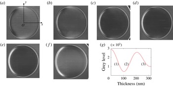
The relation between light intensity and film thickness is shown in figure 15(g): a given grey level can correspond to different heights. This appendix details our method to discriminate between the possible thicknesses. First, we determine the thickness of the film at the centre of the droplet. There, the correct branch of the intensity–thickness relation can be identified by following the variation of the intensity with
 $Ca$
, starting from a slow droplet for which the centre sits on branch (1) – see figure 15(a). Then, from figure 15(a–c), the intensity decreases as the film thickness increases along branch (1). Once the first minimum is reached, the intensity increases from figure 15(d) to (f), corresponding to a film thickening along branch (2). Then, as we move towards the front of the droplet, i.e. along the positive
 $x$
axis (
 $y=0$
), the intensity decreases in figure 15(a). This corresponds to a decrease along the right side of branch (1), and a film thickness increase. A similar analysis is made for each image. In contrast, along the positive
 $y$
axis (
 $x=0$
), the intensity increase means a shift towards the left side of branch (1) and a decrease in film thickness.
Raw images of droplets for (a)
 $Ca=7.2\times 10^{-4}$
(diameter
 $170~\unicode[STIX]{x03BC}\text{m}$
), (b)
 $Ca=9.5\times 10^{-4}$
(diameter
 $173~\unicode[STIX]{x03BC}\text{m}$
), (c)
 $Ca=1.3\times 10^{-3}$
(diameter
 $180~\unicode[STIX]{x03BC}\text{m}$
), (d)
 $Ca=1.5\times 10^{-3}$
(diameter
 $176~\unicode[STIX]{x03BC}\text{m}$
), (e)
 $Ca=1.8\times 10^{-3}$
(diameter
 $174~\unicode[STIX]{x03BC}\text{m}$
) and (f)
 $Ca=2\times 10^{-3}$
(diameter
 $195~\unicode[STIX]{x03BC}\text{m}$
). (g) Light intensity as a function of the film thickness, deduced from the optical model detailed in Huerre et al. (Reference Huerre, Jullien, Theodoly and Valignat2016).

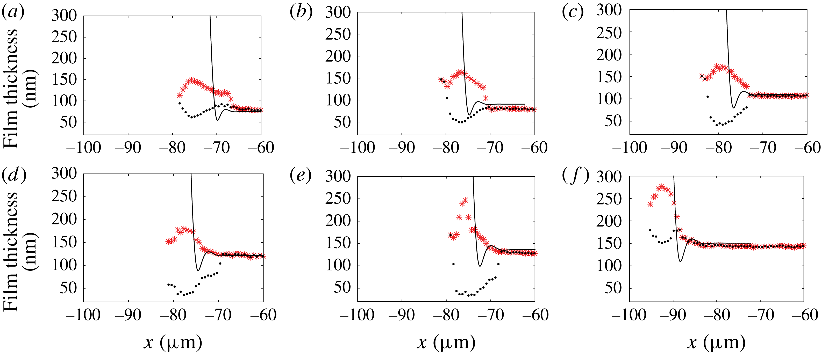
In contrast to the monotonic behaviour at the front end, a crescent-like pattern is visible at the rear in figure 15(a), where the light intensity varies over the whole range of grey levels. This makes the identification of the thickness a priori ambiguous. Moreover, the topography involves a local extremum (the middle of the crescent), so that the line level continuity cannot be used to remove the ambiguity. In figure 15(a), for instance, the isolated bright crescent surrounded by dark pixels can either be a ravine (branch (1)) or a bump (branch (2)). To remove uncertainty, the two possible thickness profiles are shown in figure 16 for different
 $Ca$
. Since the thickness is expected to vary monotonically for increasing capillary numbers, we can screen for the correct film profiles. In these examples, only the red stars correspond to a physical trend of film thickness evolution, and we can rule out the black dots that show a non-monotonic evolution of the film thickness with increasing
 $Ca$
.
Two possible profiles (black dots, ravine; red stars, bump) at the back of the droplet for (a)
 $Ca=7.2\times 10^{-4}$
, (b)
 $Ca=9.5\times 10^{-4}$
, (c)
 $Ca=1.3\times 10^{-3}$
, (d)
 $Ca=1.5\times 10^{-3}$
, (e)
 $Ca=1.8\times 10^{-3}$
and (f)
 $Ca=2\times 10^{-3}$
.
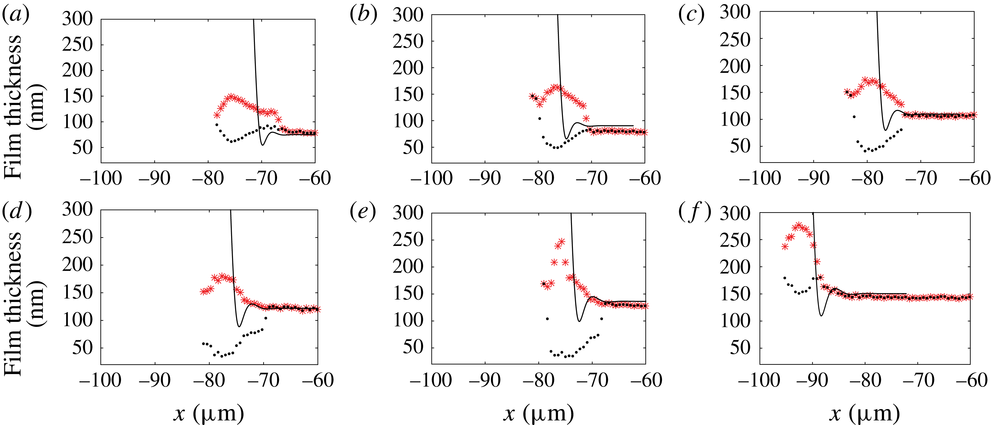
The discarded profile, showing a deep ravine (black dots), is closer to Bretherton’s theoretical prediction than the profile we selected. However, Bretherton’s solution does not recover the right radial length scale for the profile variation, and thus cannot in any case be an accurate fit to model the oscillation at the rear meniscus.
Appendix B. Lubrication equations for a circular droplet
The lubrication equation is
 $\unicode[STIX]{x1D6FB}^{2D}p=\unicode[STIX]{x1D702}\unicode[STIX]{x2202}^{2}\boldsymbol{u}/\unicode[STIX]{x2202}z^{2}$
, with the velocity
 $\boldsymbol{u}=u_{\unicode[STIX]{x1D70C}}\boldsymbol{e}_{\unicode[STIX]{x1D70C}}+u_{\unicode[STIX]{x1D703}}\boldsymbol{e}_{\unicode[STIX]{x1D703}}$
. Using the boundary condition
 $\boldsymbol{u}(0)=-U_{d}\boldsymbol{e}_{x}$
and
 $\unicode[STIX]{x2202}\boldsymbol{u}/\unicode[STIX]{x2202}z(h)=0$
we get
 $$\begin{eqnarray}\displaystyle & \displaystyle \frac{1}{\unicode[STIX]{x1D702}_{o}}\frac{\unicode[STIX]{x2202}p}{\unicode[STIX]{x2202}\unicode[STIX]{x1D70C}}=\frac{\unicode[STIX]{x2202}^{2}u_{\unicode[STIX]{x1D70C}}}{\unicode[STIX]{x2202}z^{2}}=A\quad \;\Longrightarrow \;\quad u_{\unicode[STIX]{x1D70C}}=\frac{A}{2}(z^{2}-2zh)-U_{d}\cos \unicode[STIX]{x1D703}, & \displaystyle\end{eqnarray}$$
 $$\begin{eqnarray}\displaystyle & \displaystyle \frac{1}{\unicode[STIX]{x1D702}_{o}\unicode[STIX]{x1D70C}}\frac{\unicode[STIX]{x2202}p}{\unicode[STIX]{x2202}\unicode[STIX]{x1D703}}=\frac{\unicode[STIX]{x2202}^{2}u_{\unicode[STIX]{x1D703}}}{\unicode[STIX]{x2202}z^{2}}=A^{\prime }\quad \;\Longrightarrow \;\quad u_{\unicode[STIX]{x1D703}}=\frac{A^{\prime }}{2}(z^{2}-2zh)+U_{d}\sin \unicode[STIX]{x1D703}. & \displaystyle\end{eqnarray}$$
The flux
 $\boldsymbol{Q}=\int _{0}^{h}\boldsymbol{u}\,\text{d}z$
is given by
 $$\begin{eqnarray}\displaystyle \boldsymbol{Q} & = & \displaystyle \displaystyle \left(-\frac{A}{3}h^{3}-U_{d}h\cos \unicode[STIX]{x1D703}\right)\boldsymbol{e}_{\unicode[STIX]{x1D70C}}+\left(-\frac{A^{\prime }}{3}h^{3}+U_{d}h\sin \unicode[STIX]{x1D703}\right)\boldsymbol{e}_{\unicode[STIX]{x1D703}},\end{eqnarray}$$
 $$\begin{eqnarray}\displaystyle \text{div}(\boldsymbol{Q}) & = & \displaystyle 0=\displaystyle \frac{1}{\unicode[STIX]{x1D70C}}\frac{\unicode[STIX]{x2202}(\unicode[STIX]{x1D70C}Q_{\unicode[STIX]{x1D70C}})}{\unicode[STIX]{x2202}\unicode[STIX]{x1D70C}}+\frac{1}{\unicode[STIX]{x1D70C}}\frac{\unicode[STIX]{x2202}Q_{\unicode[STIX]{x1D703}}}{\unicode[STIX]{x2202}\unicode[STIX]{x1D703}}\end{eqnarray}$$
 $$\begin{eqnarray}\displaystyle & = & \displaystyle -\frac{Ah^{3}}{3\unicode[STIX]{x1D70C}}-\frac{1}{3}\frac{\unicode[STIX]{x2202}(Ah^{3})}{\unicode[STIX]{x2202}\unicode[STIX]{x1D70C}}-\frac{U_{d}h\cos \unicode[STIX]{x1D703}}{\unicode[STIX]{x1D70C}}-U_{d}\cos \unicode[STIX]{x1D703}\frac{\unicode[STIX]{x2202}h}{\unicode[STIX]{x2202}\unicode[STIX]{x1D70C}}-\frac{1}{3\unicode[STIX]{x1D70C}}\frac{\unicode[STIX]{x2202}(A^{\prime }h^{3})}{\unicode[STIX]{x2202}\unicode[STIX]{x1D703}}\nonumber\\ \displaystyle & & \displaystyle +\,\frac{U_{d}\sin \unicode[STIX]{x1D703}}{\unicode[STIX]{x1D70C}}\frac{\unicode[STIX]{x2202}h}{\unicode[STIX]{x2202}\unicode[STIX]{x1D703}}+\frac{U_{d}h\cos \unicode[STIX]{x1D703}}{\unicode[STIX]{x1D70C}}.\end{eqnarray}$$
Assuming
 $Ah^{3}/\unicode[STIX]{x1D70C}\ll \unicode[STIX]{x2202}(Ah^{3})/\unicode[STIX]{x2202}\unicode[STIX]{x1D70C}$
and
 $(1/\unicode[STIX]{x1D70C})\unicode[STIX]{x2202}(A^{\prime }h^{3})/\unicode[STIX]{x2202}\unicode[STIX]{x1D703}\ll \unicode[STIX]{x2202}(Ah^{3})/\unicode[STIX]{x2202}\unicode[STIX]{x1D70C}$
, we get the Reynolds equation
 $$\begin{eqnarray}U_{d}\cos \unicode[STIX]{x1D703}\frac{\unicode[STIX]{x2202}h}{\unicode[STIX]{x2202}\unicode[STIX]{x1D70C}}-\frac{U_{d}\sin \unicode[STIX]{x1D703}}{\unicode[STIX]{x1D70C}}\frac{\unicode[STIX]{x2202}h}{\unicode[STIX]{x2202}\unicode[STIX]{x1D703}}+\frac{1}{3}\frac{\unicode[STIX]{x2202}Ah^{3}}{\unicode[STIX]{x2202}\unicode[STIX]{x1D70C}}=0,\end{eqnarray}$$
where
 $A$
is given by Laplace’s law
 $A=(1/\unicode[STIX]{x1D702}_{o})(\unicode[STIX]{x2202}p/\unicode[STIX]{x2202}\unicode[STIX]{x1D70C})=-(\unicode[STIX]{x1D6FE}/\unicode[STIX]{x1D702}_{o})(\unicode[STIX]{x2202}^{3}h/\unicode[STIX]{x2202}\unicode[STIX]{x1D70C}^{3})$
.
Appendix C. Disjoining pressure contribution
In the range of confinement that is investigated using microfluidics, the thin liquid film squeezed between the droplet and the wall may be so thin that intermolecular interactions come into play and may set the lubrication film thickness (Huerre et al. Reference Huerre, Theodoly, Leshansky, Valignat, Cantat and Jullien2015). In a static configuration, our experimental set-up can even be used to build disjoining pressure isotherms where the pressure is set by the level of confinement, allowing one to investigate high pressures thanks to small cavity thicknesses. The film thickness is measured using RICM (Huerre et al. Reference Huerre, Valignat, Maggs, Theodoly and Jullien2017). In these two previous works, the dominant contribution of the intermolecular interaction was due to electrostatic interactions. Under such experimental conditions, the flow in the thin liquid film is given, using the lubrication approximation, by
 $$\begin{eqnarray}\frac{\unicode[STIX]{x2202}}{\unicode[STIX]{x2202}x}\left(\unicode[STIX]{x1D6FE}\frac{\unicode[STIX]{x2202}^{2}h}{\unicode[STIX]{x2202}x^{2}}+\unicode[STIX]{x1D6F1}_{disj}\right)=-\unicode[STIX]{x1D702}_{0}\frac{\unicode[STIX]{x2202}^{2}u}{\unicode[STIX]{x2202}z^{2}},\end{eqnarray}$$
where
 $\unicode[STIX]{x1D6FE}\unicode[STIX]{x2202}^{2}h/\unicode[STIX]{x2202}x^{2}$
is the Laplace pressure,
 $u$
is the
 $x$
component of the velocity in the droplet’s frame, and
 $\unicode[STIX]{x1D6F1}_{disj}$
is the disjoining pressure given by
 $$\begin{eqnarray}\unicode[STIX]{x1D6F1}_{disj}=\unicode[STIX]{x1D6F1}_{elec}+\unicode[STIX]{x1D6F1}_{vdW}^{\unicode[STIX]{x1D708}=0}+\unicode[STIX]{x1D6F1}_{vdW}^{\unicode[STIX]{x1D708}>0},\end{eqnarray}$$
where
 $\unicode[STIX]{x1D6F1}_{elec}=64nk_{B}T\tanh (e\unicode[STIX]{x1D6F9}_{1}/k_{B}T)\tanh (e\unicode[STIX]{x1D6F9}_{2}/k_{B}T)\exp (-h/\unicode[STIX]{x1D706}_{D})$
is the entropic contribution of the electrostatic interaction (Israelachvili Reference Israelachvili2011), where
 $n$
is the ion bulk concentration,
 $k_{B}$
is the Boltzmann constant,
 $T$
is the temperature,
 $e$
is the charge of an electron,
 $\unicode[STIX]{x1D706}_{D}$
is the Debye length and
 $\unicode[STIX]{x1D6F9}_{i}$
is the potential of interface
 $i$
. For the sake of simplicity, we consider an upper limit of this contribution by taking
 $\tanh (e\unicode[STIX]{x1D6F9}_{1}/k_{B}T)\tanh (e\unicode[STIX]{x1D6F9}_{2}/k_{B}T)=-1$
. Here
 $\unicode[STIX]{x1D6F1}_{vdW}^{\unicode[STIX]{x1D708}=0}=\exp (-h/\unicode[STIX]{x1D706}_{D})A_{\unicode[STIX]{x1D708}=0}/(6\unicode[STIX]{x03C0}h^{3})$
is the van der Waals interaction at zero frequency, and
 $\unicode[STIX]{x1D6F1}_{vdW}^{\unicode[STIX]{x1D708}>0}=A_{\unicode[STIX]{x1D708}>0}/(6\unicode[STIX]{x03C0}h^{3})$
is the van der Waals dispersion contribution. For a droplet at rest, the disjoining pressure sets the film thickness, which is balanced by the Laplace pressure
 $\unicode[STIX]{x1D6FE}/H_{0}\sim 2~\text{kPa}$
(see figure 17
a). In our experimental configuration, the surfactant that we use is charged positively, and the glass substrate is charged negatively, leading to an attractive electrostatic interaction. In order to avoid such interactions, the Debye layers are purposely screened by adding salt in the external phase such that the Debye length is reduced to
 $\unicode[STIX]{x1D706}_{d}=0.2~\text{nm}$
. At rest, the estimated film thickness from figure 17 would be 5 nm. Such a small film thickness is explained in our experimental configuration by both a high confinement (small
 $H_{0}$
), leading to high pressures as noted in Huerre et al. (Reference Huerre, Valignat, Maggs, Theodoly and Jullien2017), and a small Debye length (0.2 nm). The fact that we experimentally observe film thicknesses above 40 nm in all the reported experiments shows that the film thickness is monitored by hydrodynamics. As such, a film thickness approximately 40 nm corresponds to a disjoining pressure of approximately 4 Pa (figure 17
b), a value that is three orders of magnitude lower than the capillary suction given by the Laplace pressure. We believe that disjoining pressure effects can be comfortably neglected in (C 1) and lie within the error bars.
(a) The van der Waals and electrostatic (
 $\unicode[STIX]{x1D6FC}=-64nk_{B}T$
) contributions to the total disjoining pressure
 $\unicode[STIX]{x1D6F1}_{disj}$
. The red horizontal line represents the imposed confinement pressure
 $\unicode[STIX]{x1D6FE}/H_{o}$
. (b) Zoom of the previous graph. Both imposed pressure and disjoining pressure are equal at equilibrium, leading to an equilibrium film thickness of 5 nm (intersection of the two curves).