1. Introduction
1.1. Turbulence in stratified fluids
Turbulence in oceans and atmospheres is episodic and there is general interest in the evolution and decay of localized patches of turbulence with varying degrees of turbulent kinetic energy compared with the buoyancy forces exerted by the background density gradient. The stratified ambient significantly affects the late-time evolution, assuring the emergence and longevity of coherent structures with a large ratio of horizontal to vertical length scales, and the concomitant possible endurance of information-containing patterns. Understanding the processes responsible for the initial emergence of such patterns is important for predictive geophysical studies and modelling and also to potential or hopeful pattern detectors (Spedding Reference Spedding2014). In addition, the general topic of long-lived and stable fluid mechanical signatures of geographical features, submerged vehicles or animals of various scales has quite broad significance. The principle of the emergence of order from initially disordered or irregular conditions is also of perennial interest (Voropayev & Afanasyev Reference Voropayev and Afanasyev1994).
Far from any boundaries, one may identify a class of oceanic and atmospheric flows where length (
 $L$
) and time (
 $L/U$
) scales are insufficiently large to be impacted by planetary rotation, but are variously modified by the constraining effect of a background density gradient. Such flows can be described in terms of Reynolds and Froude numbers,
 $$\begin{eqnarray}\mathit{Re}=\frac{UL}{{\it\nu}},\quad \mathit{Fr}=\frac{U}{NL},\end{eqnarray}$$
for kinematic viscosity
 ${\it\nu}$
and Brunt–Väisälä frequency
 $N=\sqrt{(-g/{\it\rho}_{0})\,\partial {\it\rho}/\partial z}$
(where
 $g$
is the gravitational acceleration,
 ${\it\rho}_{0}$
is a reference density and
 $\partial {\it\rho}/\partial z$
is the density gradient in the direction parallel to
 $g$
). In many geophysical and engineering applications, the product
 $UL$
is large, and so Re is commonly
 $10^{6}$
or higher. The ratio of
 $U/L$
varies, however. For an imagined flow over an island with
 $U=10~\text{m}~\text{s}^{-1}$
and
 $L=10~\text{km}$
,
 $\mathit{Re}\approx 7\times 10^{9}$
; and in a plausibly strongly stratified atmosphere with
 $N=10^{-2}~\text{rad}~\text{s}^{-1}$
,
 $\mathit{Fr}\approx 10^{-1}$
. By contrast, an equivalent estimate for a submerged body of
 $U=10~\text{m}~\text{s}^{-1}$
,
 $L=10~\text{m}$
and
 $N=10^{-3}~\text{rad}~\text{s}^{-1}$
in the ocean thermocline yields
 $\mathit{Re}\approx 10^{8}$
and
 $\mathit{Fr}\approx 10^{3}$
. Time scales associated with the initial turbulence are of order unity, which is three orders of magnitude shorter than those associated with natural buoyancy frequencies. Nevertheless, if the disturbances continue to evolve with no further energy input, then
 $L$
increases while
 $U$
decreases, so that all flows in a stratified ambient eventually find themselves in a regime where local Froude numbers are of order unity or smaller. Buoyancy eventually wins, and the only question is how and whether the turbulence parametrized by Re has evolved before reaching this terminal state.
When an initial
 $\mathit{Re}_{0}$
is small, viscosity can dampen or smooth out small-scale turbulent fluctuations before they can become of dynamical significance. There are important differences between these viscous-controlled motions, which are simple enough to produce in a laboratory experiment, and truly inertially driven but buoyancy controlled flows, which are not. A number of studies have noted that low-Re, strongly stratified turbulence has qualitatively and quantitatively different dynamics than high-Re, strongly stratified turbulence (Riley & de Bruyn Kops Reference Riley and de Bruyn Kops2003; Godoy-Diana, Chomaz & Billant Reference Godoy-Diana, Chomaz and Billant2004; Hebert & de Bruyn Kops Reference Hebert and de Bruyn Kops2006a
; Brethouwer et al.
Reference Brethouwer, Billant, Lindborg and Chomaz2007; Deloncle, Billant & Chomaz Reference Deloncle, Billant and Chomaz2008; Augier, Chomaz & Billant Reference Augier, Chomaz and Billant2012), and a buoyancy Reynolds number,
 $\mathit{Re}_{b}=\mathit{Re}\,\mathit{Fr}^{2}$
, has been used to demarcate these apparently different regimes.
If strongly stratified regimes are the ultimate destination for very many environmentally and geophysically relevant flows, the trajectory of the flow solutions in arriving at this point differs according to the generation mechanisms. Laboratory and numerical experiments attempt to set up or mimic general conditions that have some degree of universality, but the importance of initial conditions in determining even the late-time state has been a matter of some dispute. For example, while Métais & Herring (Reference Métais and Herring1989) showed that initial conditions in stratified turbulence simulations were evident even at late times, Meunier & Spedding (Reference Meunier and Spedding2006) found that almost all stratified wakes produced by bluff bodies have universal characteristics that effectively obliterate their initial (transient) conditions (see also Meunier & Spedding Reference Meunier and Spedding2004). It may be unwise to expect one simple answer to questions of the importance of initial conditions in late-time evolution of stratified flows, and a brief survey of selected old and recent experiments is illustrative in reconstructing the routes to stratified turbulence and our understanding of the same.
1.2. Experiments on stratified grid turbulence
The systematic variation of initial conditions in stratified grid turbulence began when grid arrays with characteristic mesh spacing,
 $M$
, were towed either horizontally (Lin & Veenhuizen Reference Lin and Veenhuizen1975) or vertically (Dickey & Mellor Reference Dickey and Mellor1980) through stably stratified fluids, or when closed-loop channels were used to cycle a flow past a stationary array of cylinders or rods (Stillinger, Helland & van Atta Reference Stillinger, Helland and van Atta1983; Itsweire, Helland & van Atta Reference Itsweire, Helland and van Atta1986). In the following discussion, we shall refer to
 $\{x,y,z\}$
as coordinates in the streamwise, lateral and vertical directions, with velocity components
 $\{u,v,w\}$
. Buoyancy forces act primarily in the
 $z$
direction, and so one of the simple measures is to estimate the anisotropy of
 $\{u,v\}$
components versus
 $w$
. Component
 $w$
was found to decay faster than
 $u$
, and so ratios of fluctuating
 $u^{2}/w^{2}$
were found to increase with
 $x/M$
, but at different rates, and with measurable differences starting to emerge at very different
 $x/M$
(Itsweire et al.
Reference Itsweire, Helland and van Atta1986). Though strong anisotropy could be observed without ambiguity at large
 $x/M$
, it was not clear when and how the various scales of motion were affected at small
 $x/M$
. Most data began at
 $x/M\simeq 10$
and trends at that point could be interpreted differently. The emerging consensus was that at first the turbulence immediately behind a grid evolves as it would in the absence of stratification. Gradually, the larger vertical length and velocity scales are first suppressed, and then the smaller scales. It was understood that both Re and
 $N$
(eventually expressed as Fr) were important in determining the pathway to a final state, which at the time was described as being a sea of internal waves.
The same framework was implicitly or explicitly invoked in subsequent studies (Browand, Guyomar & Yoon Reference Browand, Guyomar and Yoon1987; Hopfinger Reference Hopfinger1987; Liu, Maxworthy & Spedding Reference Liu, Maxworthy and Spedding1987) when a turbulent front was allowed to expand into a still ambient. The point at which strong anisotropy was observed was often described as a point of ‘collapse’, a terminology that seemed natural based on observations through shadowgraph imagery of the density perturbation field. Despite the fact that no quantitative measure actually decreased suddenly, as implied by the term, it remained in use, though it was realized not only that the late-time motions were internal wave fields, but also that large-scale horizontal motions would occur within separate layers.
The pancake eddies identified by Lin & Pao (Reference Lin and Pao1979) in the wakes of towed bodies were therefore also seen in the late stages of grid turbulence. Further grid turbulence experiments measured using particle imaging velocimetry (PIV)-based methods were conducted for a two-layer fluid by Yap & van Atta (Reference Yap and van Atta1993) and in some quantitative detail for a continuous linear density gradient by Fincham, Maxworthy & Spedding (Reference Fincham, Maxworthy and Spedding1996) and by Praud, Fincham & Sommeria (Reference Praud, Fincham and Sommeria2005). In the latter two sets of experiments, most observations were at moderate to late-time (
 $Nt\geqslant 10,~x/M\geqslant 5$
) motions on an isopycnal or in horizontal interrogation sheets, and so the focus was naturally on the development of the large-scale horizontal motions that dominated. The quasi-horizontal vortices filled the experimental tank, evolving slowly, but uncorrelated in the vertical.
The shearing motion between vertically uncorrelated (except through the shear itself) layers accounted for about 90 % of the kinetic energy dissipation. In both sets of experiments, the grid bars were oriented vertically so as to deliberately reduce the amplitude of the initial vertical forcing, which would otherwise quickly fill the tank with internal waves. The decorrelation of adjacent vertical layers was much as originally conjectured by Lilly (Reference Lilly1983), but the experiments were also confined to quite low values of
 $\mathit{Re}_{b}$
(see discussion in Brethouwer et al.
Reference Brethouwer, Billant, Lindborg and Chomaz2007) and so a simple extrapolation to atmospheric conditions is not justified. Attempts to extend experiments into the strongly stratified, high-
 $\mathit{Re}_{b}$
regime have been partially successful (Augier et al.
Reference Augier, Billant, Negretti and Chomaz2014) in arrangements that have a continuous forcing of a large number of initially coherent vortices, but
 $\mathit{Re}_{b}\approx 300$
was still insufficient for the development of inertial range signatures in second-order structure functions.
1.3. Computations of strongly stratified turbulence
Early computations (Riley, Metcalf & Weissman Reference Riley, Metcalf and Weissman1981; Métais & Herring Reference Métais and Herring1989) examined the evolving turbulence in terms of vortical and wave modes, and it was noted that the late-time vortical motions (what Lighthill (Reference Lighthill1996) would refer to as residual motions) would decay very slowly and evolved almost independently of the internal waves. The ratio of vortical to wave modes depended quite strongly on the strengths with which they were initialized to begin with.
Since then, simulations of box-filling stratified turbulence have exploited symmetries (or asymmetries) in initial conditions or modelling at small scales in order to push
 $\mathit{Re}_{b}$
as high as possible (Riley & de Bruyn Kops Reference Riley and de Bruyn Kops2003; Waite & Bartello Reference Waite and Bartello2004, Reference Waite and Bartello2006; Hebert & de Bruyn Kops Reference Hebert and de Bruyn Kops2006a
,Reference Hebert and de Bruyn Kops
b
; Lindborg Reference Lindborg2006; Brethouwer et al.
Reference Brethouwer, Billant, Lindborg and Chomaz2007; Waite Reference Waite2011). When and if initial conditions permit some coherence in the vertical direction, the vertical length scales can be set by zigzag modes (Billant Reference Billant2010; Billant et al.
Reference Billant, Deloncle, Chomaz and Otheguy2010), and Augier & Billant (Reference Augier and Billant2011) demonstrate how a dynamical balance is established between vertical length scales and shearing instability modes.
There has been much progress in analysis of these high-
 $\mathit{Re}_{b}$
flows to reconcile apparent contradictions in observed vertical and horizontal energy spectra in simulations and atmospheric data where simultaneous forward and inverse cascades can coexist (Lindborg Reference Lindborg2006; Brethouwer et al.
Reference Brethouwer, Billant, Lindborg and Chomaz2007; Riley & Lindborg Reference Riley and Lindborg2008).
1.4. Turbulent patches and wakes
A number of studies have concerned themselves with the evolution of turbulent patches or wakes that are then free to evolve in an otherwise quiescent ambient. Early experimental studies on wakes of bluff bodies include those by Lin, Boyer & Fernando (Reference Lin, Boyer and Fernando1992), Chomaz, Bonetton & Hopfinger (Reference Chomaz, Bonetton and Hopfinger1993), Bonneton et al. (Reference Bonneton, Chomaz, Hopfinger and Perrier1996), Spedding, Browand & Fincham (Reference Spedding, Browand and Fincham1996b ) and Spedding (Reference Spedding1997, Reference Spedding2002). A general picture emerged of three regimes, where an initial three-dimensional (3D) turbulence adjusts to the background buoyancy forcing through an intermediate non-equilibrium (NEQ) regime, which later evolves in mostly horizontal quasi-two-dimensional (Q2D) motions that decay slowly and maintain a very stable geometry of coherent vortical structures. Their slow decay is quite consistent with the earlier computations and predictions of Riley et al. (Reference Riley, Metcalf and Weissman1981). While plausible that these NEQ–Q2D transitions are consistent with the instability mechanisms successfully generalized by Billant (Reference Billant2010) and Billant et al. (Reference Billant, Deloncle, Chomaz and Otheguy2010), detailed examination is difficult because the initial conditions themselves are not prescribed with great precision.
There was some initial uncertainty about whether the observed wakes were peculiar to spheres, or other conditions and symmetries on the body, but early direct numerical and large-eddy simulations of high-Re wake-like initial conditions (where turbulence is superimposed upon a given mean flow profile) showed that satisfactorily similar phenomena could be generated with no body at all (Gourlay et al. Reference Gourlay, Arendt, Fritts and Werne2001; Dommermuth et al. Reference Dommermuth, Rottman, Innis and Novikov2002; Diamessis, Domaradzki & Hesthaven Reference Diamessis, Domaradzki and Hesthaven2005). Experiments on the spread of turbulent patches in a stratified background were broadly consistent with the late-wakes descriptions but do not show the same regular Q2D vortex arrays (Fernando Reference Fernando1988; De Silva & Fernando Reference De Silva and Fernando1992) since there are no mean-shear initial conditions to set it up.
Though Meunier & Spedding (Reference Meunier and Spedding2004, Reference Meunier and Spedding2006) contend that there are universal aspects of these momentum wakes that cross all likely initial conditions, quantitative and detailed experiments have not been made to test how useful the idea may be in decaying and spreading grid turbulence, with no special body or initial conditions to drive particular symmetries.
As DNS can extend to higher
 $\mathit{Re}_{b}$
, the possibility has been raised that energetic secondary instabilities of the developing shear layers in strongly stratified turbulence (Riley & de Bruyn Kops Reference Riley and de Bruyn Kops2003; Hebert & de Bruyn Kops Reference Hebert and de Bruyn Kops2006a
; Diamessis, Spedding & Domaradzki Reference Diamessis, Spedding and Domaradzki2011) provide a further barrier to extrapolating laboratory experiments to higher Re, and so it is interesting to consider experimental devices that may eventually reach high-
 $\mathit{Re}_{b}$
regimes (Augier et al.
Reference Augier, Billant, Negretti and Chomaz2014). The different initial conditions can also be compared in similar frameworks, experimental or computational (e.g. Pal, de Stadler & Sarkar Reference Pal, de Stadler and Sarkar2013).
1.5. Objectives
The detailed and fine-grained purpose of this study is to use a towed grid to generate a disturbance that shares some wake characteristics, along with varying initial turbulence intensities, so the evolution with distance from the grid (or wake age) may be traced to provide an example of a turbulent field adjusting to the background density gradient. The grid has a circular cross-section and a square mesh with equal spacing in the horizontal and vertical directions, so the initial disturbance/forcing is also of equal magnitude in
 $\{y,z\}$
. The experiments are performed in a refractive-index-matched fluid, and special care is taken to resolve mean and fluctuating quantities in both instantaneous and time-averaged measures.
The general idea is that the detailed and quantitative study of the first stages of stratified grid turbulence can shed some light as to how the well-studied late turbulence stages emerge, and how well this one example conforms to a general model of initial turbulence in a stably stratified background.
2. Experimental methods
2.1. Physical set-up
Experiments were conducted by towing a circular grid of radius
 $R=4~\text{cm}$
and square mesh spacing,
 $M=3.2~\text{mm}$
, on 0.45 mm diameter bars (so the solidity is 26 %) in a
 $0.80^{3}~\text{m}$
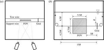
tank. The grid orientation was maintained using support and tow wires (of 1.14 mm diameter) as shown in figure 1. The tow and support wires were attached to the grid at diametrically opposite points on its circumference to assure steady translation motion only. The centre measurement plane is not directly disturbed by the wires. The fluid depth
 $H=35~\text{cm}$
, so the grid was
 $4.5R$
from the free surface and
 $4.25R$
from the bottom of the tank. The grid was towed at speeds
 $U=\{6.8,14.3,27.6\}~\text{cm}~\text{s}^{-1}$
, through a total distance of
 $15R$
, entering the field of view (FOV) after
 $5R$
so as to avoid transients from start-up. Subsequent measurements of statistics in mean and turbulence quantities over left (new) and right (old) parts of the flow field, either time- or space-averaged, revealed no significant or systematic differences. The temperature of the fluid was maintained at 22 °C and the average kinematic viscosity was
 ${\it\nu}=1.005\times 10^{-6}~\text{m}^{2}~\text{s}^{-1}$
.
 $\mathit{Re}$
ranged from 2700 to 11 000, for
 $N$
between
 $0.2\leqslant N\leqslant 2.8~\text{rad}~\text{s}^{-1}$
, and
 $\mathit{Fr}$
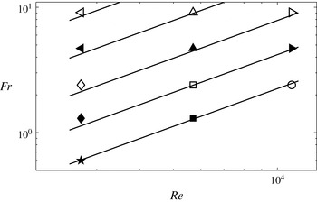
varied over 0.6–9.1. Figure 2 shows the resulting
 $\{\mathit{Fr}{-}\mathit{Re}\}$
parameter space.
Sketch of towed grid experiment: (a) top view and (b) side view.

The
 $\mathit{Fr}{-}\mathit{Re}$
parameter space. Straight lines from top to bottom indicate
 $\mathit{Fr}{-}\mathit{Re}$
pairs with
 $N=\{0.2,0.4,0.8,1.5,2.8\}$
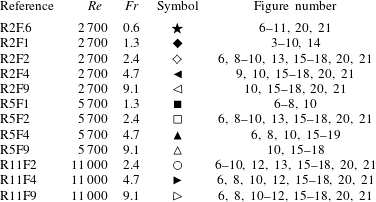
, respectively. The symbols represent experiments listed in table 1. These symbol conventions will be used consistently throughout the paper.

The
 $\mathit{Re}$
and
 $\mathit{Fr}$
values for all experiments, with symbols corresponding to figure 2. The last column lists the figure in which each run appears. The symbols are consistent throughout.

2.2. Data acquisition
Three components of velocity in a two-dimensional plane (3C2D) were estimated using a stereoscopic PIV system from LaVision. Two matching cameras (LaVision-Imager sCMOS) with a resolution of
 $2560~\text{pixel}\times 2160~\text{pixel}$
were driven at a 40 Hz base rate. The measurement plane was illuminated by an Nd:YAG laser (LaVision NANO L100-50PIV), pulsed also at 40 Hz. The laser beam is spread into a sheet with a thickness of about 2 mm in the test section. In most cases the flow was seeded with
 $20\,{\rm\mu}\text{m}$
diameter polyamide particles (Dantec Dynamics PSP-20) with an average density of
 $1.03~\text{g}~\text{cm}^{-3}$
. At the highest stratification when
 $N=2.8$
, titanium dioxide particles with average density of
 $4.23~\text{g}~\text{cm}^{-3}$
and diameter
 $15~{\rm\mu}\text{m}$
were substituted. Images were processed with the multi-pass cross-correlation algorithm with window deformation and shift of 50 %, and with interrogation window sizes varying from
 $128~\text{pixel}\times 128~\text{pixel}$
to
 $32~\text{pixel}\times 32~\text{pixel}$
.
2.3. Refractive index matching
The standard two-tank method was used to establish a linear density gradient, and the refractive index was held constant at any density by systematically varying the concentrations of both evaporated salt (Ca- and Mg-free) and ethanol (200 proof) solutions. A modified version of the refractive-index-matching (RIM) technique (summarized by Daviero, Roberts & Maile (Reference Daviero, Roberts and Maile2001)) was implemented for a broad variation of densities. An empirical relationship between density and concentration at 20 °C for salt solution was provided by Weast & Lide (Reference Weast and Lide1989), and that for ethanol solution by Perry, Green & Maloney (Reference Perry, Green and Maloney1997). They can be approximated by quadratic fits as
 $$\begin{eqnarray}\displaystyle & \text{salt }{\it\rho}_{s}=2.46\times 10^{-5}C_{s}^{2}+0.0070C_{s}+0.9982, & \displaystyle\end{eqnarray}$$
 $$\begin{eqnarray}\displaystyle & \text{ethanol }{\it\rho}_{e}=-7.9\times 10^{-6}C_{e}^{2}-0.0013C_{e}+0.9982, & \displaystyle\end{eqnarray}$$
 $C_{s}$
and
 $C_{e}$
are the concentrations of salt and ethanol, and
 ${\it\rho}_{s}$
and
 ${\it\rho}_{e}$
are the densities of salt and ethanol solutions, respectively. When
 $C_{e}\leqslant 0.35$
, there is an approximately linear response in refractive index to changes in concentration. In this range, the refractive-index dependence on concentration is provided by Weast & Lide (Reference Weast and Lide1989), and approximated using a linear fit as
 $$\begin{eqnarray}\displaystyle \text{salt }n_{s} & = & \displaystyle 1.77\times 10^{-3}C_{s}+1.3330,\end{eqnarray}$$
 $$\begin{eqnarray}\displaystyle \text{ethanol }n_{e} & = & \displaystyle 6.81\times 10^{-4}C_{e}+1.3330,\end{eqnarray}$$
 $n_{s}$
and
 $n_{e}$
are the refractive indices of salt and ethanol solutions, respectively.
Based on these relations, salt and ethanol solutions that are theoretically refractive-index-matched were prepared with a specific density difference. Further verification and refinement of RIM was achieved by observing the deflection of a small laser pointer beam after passing through a transparent triangular container with the two solutions, and/or their mixture. The relative uncertainty in refractive index
 ${\rm\Delta}n/n<1\times 10^{-4}$
. The heavy-side tank of the two tanks was filled with only salt solution, and the light-side tank was filled with the required mixture of salt and ethanol to yield the required density difference and corresponding
 $N$
.
There can be quite large variations in kinematic viscosity in the strongest stratifications, with
 ${\it\delta}{\it\nu}/{\it\nu}\approx 0.2$
over a vertical distance of
 $4R$
around the wake centre when
 $N=2.8$
. The prediction and estimation of
 ${\it\nu}$
is quite uncertain at high concentrations, when the
 ${\it\mu}(C_{e})$
curves can be nonlinear and non-monotonic, and the chemistry of their combinations is not necessarily simple. The maximum difference in
 $\mathit{Re}$
depends on
 ${\it\delta}{\it\rho}$
as well as on
 ${\it\delta}{\it\nu}$
, and is about 10 % across the wake, which does not typically move the data from one significantly different regime to another (experiments are compared across factors of 2 or 4 in Re). Furthermore, local wake averages use both upper and lower wake edges to derive the quantitative statistics.
Finally, we note that the RIM considerably complicates many standard methods of density estimation, and renders all current optical whole-field methods unusable. Methods for overcoming these difficulties are being tested, but there are no local (for example, at the wake edge, or its interior) measures of density in the current data, only bulk estimates from samples withdrawn before and after experiments.
2.4. Analysis
Velocity components
 $\{u,v,w\}$
are available over
 $\{x,z\}$
in the centreplane
 $y=0$
and at
 $1/20~\text{s}$
intervals. In the lee of the towed grid, for small
 $x/R$
and small
 $x/M$
, there is no good reason to search for, or assume, self-similar characteristics, and one searches for local measures that are appropriate for preserving local pattern and geometry if it exists in some reference frame. As a start, one may consider either spatial,
 $$\begin{eqnarray}\langle q\rangle (\boldsymbol{x}_{0},t_{l0})=\frac{1}{{\rm\Delta}L}\int _{L_{1}}^{L_{2}}q(\boldsymbol{x}=(x,z_{0}),t_{l0})\,\text{d}x,\end{eqnarray}$$
or temporal,
 $$\begin{eqnarray}\overline{q}(\boldsymbol{x}_{0})=\frac{1}{{\rm\Delta}{\it\tau}}\int _{{\it\tau}_{1}}^{{\it\tau}_{2}}q(\boldsymbol{x}=(x_{0},z_{0}),t_{l})\,\text{d}t_{l},\end{eqnarray}$$
averaging, so the variables
 $\langle q\rangle$
,
 $\overline{q}$
and
 $q$
are spatially and temporally averaged, and instantaneous flow field quantities, respectively. Here
 $\boldsymbol{x}_{0}$
is downstream position with coordinates
 $(x_{0},z_{0})$
, with origin at the centre of the towed body. The averaging time and length scales are
 ${\rm\Delta}{\it\tau}={\it\tau}_{2}-{\it\tau}_{1}$
and
 ${\rm\Delta}L=L_{2}-L_{1}$
, respectively, and
 $x_{0}=(L_{2}+L_{1})/2$
. Note that
 $t_{l}$
is laboratory time, whereas
 $t$
is defined locally for every vertical slice as the time elapsed since the grid passed that vertical slice. Therefore
 $Nt$
corresponds to
 $x/R$
through the relation
 $x/R=Nt\,\mathit{Fr}$
.
For spatial averaging to be valid, the averaging distance
 ${\rm\Delta}L$
must be small compared with characteristic streamwise length scales in the flow, which is reasonable at large
 $x_{0}$
or, equivalently,
 $Nt$
:
 $$\begin{eqnarray}\frac{{\rm\Delta}L}{x_{0}}=\frac{{\rm\Delta}L/R}{Nt\,\mathit{Fr}}\ll 1.\end{eqnarray}$$
While this approximation is widely used to describe the late wake (Spedding, Browand & Fincham Reference Spedding, Browand and Fincham1996a ), it is not appropriate for the near wake, so all averaged results described here (and denoted with an overbar) are temporal averages in a frame of reference that moves with the grid.
The root-mean-square (r.m.s.) fluctuating quantity based on temporal averaging is
 $$\begin{eqnarray}q^{\prime }(\boldsymbol{x}_{0})=\left[\frac{1}{{\rm\Delta}{\it\tau}}\int _{{\it\tau}_{1}}^{{\it\tau}_{2}}[q(\boldsymbol{x}_{0},t_{l})-\overline{q}(\boldsymbol{x}_{0})]^{2}\,\text{d}t_{l}\right]^{1/2}.\end{eqnarray}$$
Finally, to ensure sufficient samples for convergence of both mean and fluctuating quantities, temporal averaging is performed on the data from each run and then ensemble-averaged over 16 runs. The combined result is for columnwise statistics that have up to 900 elements (the precise number varies with
 $x$
).
3. Results
3.1. Instantaneous and time-averaged wake structure
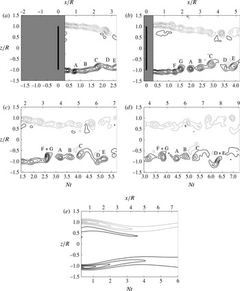
Figure 3 shows the normalized lateral vorticity,
 ${\it\omega}_{y}/N(x,z)$
, at four different times with the measurement window fixed in the laboratory reference frame. Note how the
 $Nt=x/R=0$
origin moves with the grid. At the wake edge,
 ${\it\omega}_{y}$
develops in shear layers, while in the interior wake region, the flow is relatively uniform. The trailing vortices drift slowly upstream, growing larger and weaker through diffusion and/or merging, and then begin to lose coherence as they occupy the wake interior. The wake contracts in the vertical direction, reaching a minimum height at
 $3\leqslant Nt\leqslant 4$
before expanding again. This wake contraction is observed at all
 $\{\mathit{Re},\mathit{Fr}\}$
. As
 $\mathit{Fr}$
increases, the minimum wake height occurs at a larger
 $x/R$
, but still at
 $3\leqslant Nt\leqslant 4$
.
(a–d) Four snapshots of
 ${\it\omega}_{y}/N$
for
 $\mathit{Fr}=1.3$
and
 $\mathit{Re}=2700$
(R2F1, ♦). Minimum contour levels,
 $|c_{min}|=\pm 1$
, and contour spacing,
 ${\rm\Delta}c=1$
. The evolution and interaction of individual vortices is given by letter labels, based on the full time resolution series. The shaded region is not accessible to both cameras. (e) A time average,
 $\overline{{\it\omega}}_{y}/N$
(
 $|c_{min}|=\pm 0.5,~{\rm\Delta}c=0.5$
).

The local flow characteristics can be discerned from the evolution of the individual vortices, which are tracked and marked by letters A to G in the figure. The initial shear layer evolves into discrete vortices similar to A, B and C. Vortices D and E, as well as F and G, show the pairing–merging process. In the grid-based reference frame, any given vortex appears at larger
 $Nt$
or
 $x/R$
as wall clock time increases. The time-averaged lateral vorticity,
 $\overline{{\it\omega}}_{y}/N$
, therefore preserves the overall wake geometry and its contraction, which is fixed with respect to the grid, but not the individual vortex histories, which are not.
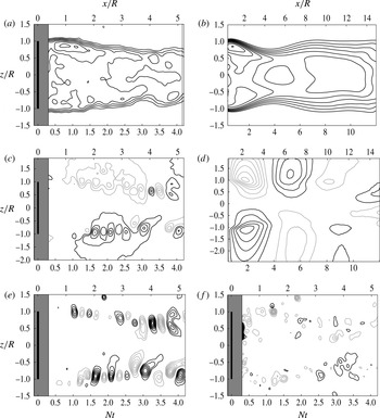
The dynamics of the near wake can also be illustrated by the various velocity component fields separately. Instantaneous and time-averaged streamwise velocity fields are given in figure 4(a,b). The pinching of the isocontours at the location of highest
 $\partial u/\partial z$
coincides with the position of the first vortices in figure 3(a), commensurate with their Kelvin–Helmholtz (KH) origin.
Instantaneous and mean velocity field components: (a)
 $u/U$
, (b)
 $\overline{u}/U$
, (c)
 $w/U$
, (d)
 $\overline{w}/U$
, (e)
 $(w-\overline{w})/U$
and ( f)
 $v/U$
for
 $\mathit{Fr}=1.3$
and
 $\mathit{Re}=2700$
(R2F1, ♦). (Here
 $|c_{min}|=\pm \{0.1,0.06,0.05,0.02,0.04,0.06\}$
and
 ${\rm\Delta}c=\{0.1,0.06,0.05,0.02,0.02,0.06\}$
.)

The wake contraction is clear in both mean and instantaneous fields, but the time-averaged fields have more broadly spread contours after it, as the locations of maximum
 $\partial u/\partial z$
vary in
 $z$
. The contraction itself is associated with a mean upwards/downwards inflow in both instantaneous (figure 4
c) and mean (figure 4
d) vertical velocity fields, from which it is clear that the vertical disturbances have moved much further from the wake centre than have the streamwise disturbances. The mean vertical flows do not average out to zero but maintain a coherent structure, which therefore is moving at the speed of the grid. The remaining fluctuations in
 $w$
(figure 4
e) stay at the wake edge, characterized by alternating-sign contours, associated with the vortex structures there, and do not propagate outwards. The instantaneous out-of-plane (or lateral) component of velocity,
 $v/U$
, is mainly incoherent and drawn in coarse detail only in figure 4( f). The association of coherent regions of lateral motion with wake-edge vortices begins only towards the later stages where
 $Nt>4$
.
3.2. Mean and turbulence profiles
3.2.1. Wake height and lee waves
To form appropriate averaged measures in the near wake, the wake geometry and length scales must be specified and measured in terms that do not presume self-similarity of mean or turbulent velocity profiles. The most clear signal comes from
 $\overline{{\it\omega}}_{y}$
(shown in figure 3
e) and profiles of
 $\overline{{\it\omega}}_{y}(z)$
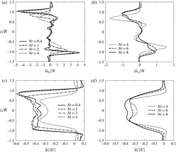
(shown for a range of
 $Nt$
in figure 5). The decay of the peak
 $\overline{{\it\omega}}_{y}$
can be observed by tracking the amplitude of crests, and their diffusion is noted in the increasing width of the crests. The peaks occur closer to the wake centre as
 $Nt$
increases up to
 $Nt=4$
and the trend is reversed for
 $Nt\geqslant 4$
. The crests roughly correspond to the locations of the maximum velocity gradient, as can be seen in figure 5(c,d). The redistribution of turbulent kinetic energy from wake edge to centre (see figure 3) is responsible for the changing shape of
 $\overline{u}$
, as the relatively irregular shape evolves into a more Gaussian-like profile at late time.
Plots of
 $\overline{{\it\omega}}_{y}/N$
at specific
 $Nt$
, for
 $\mathit{Fr}=1.3$
and
 $\mathit{Re}=2700$
(R2F1, ♦).

The crests of
 $\overline{{\it\omega}}_{y}$
may be used to define the edge of the wake, and the distance between the top and bottom crests defines a wake height,
 $2h(Nt)$
. Though this procedure will eventually fail when the vortices dissipate due to viscosity, it is robust in the near-wake region. The dimensionless wake half-height is defined as
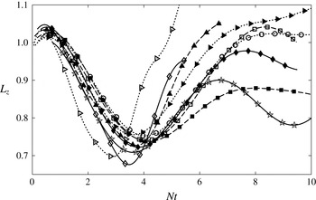
 $L_{z}=h/R$
, and is shown as a function of
 $Nt$
in figure 6.
PLot of
 $L_{z}(Nt)$
, with least-squares sine series fit. Solid, dashed and dotted lines are for
 $\mathit{Re}=\{2700,5700,11\,000\}$
respectively; the various symbols correspond to the cases shown in table 1. The solid line with ♦ corresponds to R2F1 shown in figure 5. Data points are subsampled for clarity.

The minimum values,
 $L_{z,min}$
, for all curves lie between
 $3\leqslant Nt\leqslant 4$
independent of
 $\mathit{Fr}$
and
 $\mathit{Re}$
. If
 ${\it\lambda}$
is a wavelength in
 $x$
, it may be written as
 $$\begin{eqnarray}\frac{{\it\lambda}}{R}=\frac{U\,Nt_{{\it\lambda}}}{NR}=\mathit{Fr}\,Nt_{{\it\lambda}},\end{eqnarray}$$
where
 $Nt_{{\it\lambda}}$
is the wavelength in
 $Nt$
. There is a linear relationship between
 ${\it\lambda}/R$
and
 $\mathit{Fr}$
, with slope
 $Nt_{{\it\lambda}}$
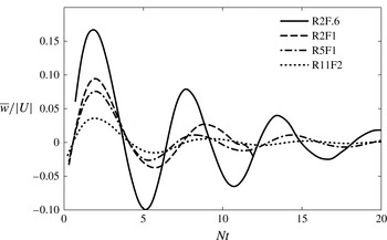
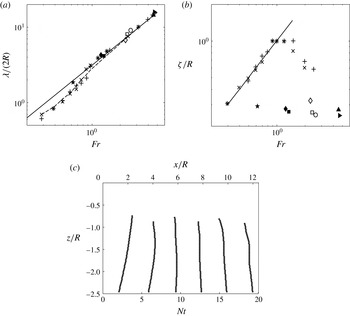
. The wave pattern is more pronounced when plotted locally at the wake edge as in figure 7. By measuring the
 ${\rm\Delta}Nt$
between the first trough and first crest,
 ${\it\lambda}/R$
is calculated using (3.1) and shown in figure 8(a). The results agree well with the linear theory prediction,
 $Nt_{{\it\lambda}}=N\times 2{\rm\pi}/N=2{\rm\pi}$
. As
 $Nt_{{\it\lambda}}$
is associated with the wake contraction, then we may infer it to be a consequence of a steady lee wave behind the grid, with wavelength independent of
 $\mathit{Re}$
. Such a result is also consistent with experiments in Chomaz et al. (Reference Chomaz, Bonetton and Hopfinger1993) and the simulations in Hanazaki (Reference Hanazaki1988) for sphere wakes with
 $\mathit{Fr}>1$
.
Plot of
 $\overline{w}/U$
at the wake edge.

(a) Plot of
 ${\it\lambda}/R$
versus
 $\mathit{Fr}$
:
 $+$
and
 $\times$
, experimental results of Chomaz et al. (Reference Chomaz, Bonetton and Hopfinger1993), with
 $\mathit{Re}=2177$
and 4514, respectively; solid line,
 ${\it\lambda}/R=2{\rm\pi}\mathit{Fr}$
; dashed line, numerical simulation of Hanazaki (Reference Hanazaki1988); other symbols, selected results from this study, see table 1 for
 $\mathit{Re}$
and
 $\mathit{Fr}$
. (b) Plot of
 ${\it\zeta}/R$
versus
 $\mathit{Fr}$
: solid line,
 $2{\it\zeta}/R=\mathit{Fr}$
; other symbols are from the same data source as panel (a). (c) Lee-wave isophase curves (every
 ${\rm\pi}$
) in the vertical centre plane, for R2F.6 (
 $\bigstar$
).

By inspection of figure 6, the wave amplitude, plotted in figure 8(b), appears to have no systematic dependence on either
 $\mathit{Re}$
or
 $\mathit{Fr}$
. This contrasts sharply with the sphere case shown by Chomaz et al. (Reference Chomaz, Bonetton and Hopfinger1993), where the scaled amplitude
 ${\it\zeta}/R$
increased linearly in the near wake with
 $\mathit{Fr}$
for
 $\mathit{Fr}\in [0.3,0.8]$
, had maximum amplitude
 ${\it\zeta}/R=1$
for
 $\mathit{Fr}\in [0.8,1.5]$
, and decreased slowly with
 $\mathit{Fr}$
after that. Here, the wave amplitude is disconnected from the outer length scale,
 $R$
, of the grid because fluid particles in the midline, for example, are never obliged to turn over the grid, instead passing straight through. This is a straightforward demonstration of how near-wake geometry can and must depend on the initial and boundary conditions.
The lee waves propagate into the exterior, and isophase lines can be drawn from the zero-crossings of the vertical velocity component. These lines are shown for the lower half-plane in figure 8(c). Similar isophase lines were also reported by Chomaz et al. (Reference Chomaz, Bonetton and Hopfinger1993) for the sphere wake.
The mix of grid permeability and vertical wave motions induced by the partial blockage leads to some interesting effects on the wake. When
 ${\it\lambda}$
is small, at low
 $\mathit{Fr}$
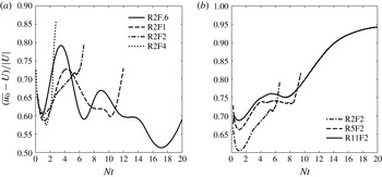
, even the inner wake region is influenced by the lee wave, as it reduces the effective wake area, somewhat akin to a nozzle in a jet. Figure 9(a) shows the mean streamwise centreline velocity,
 $\overline{u}_{0}$
, relative to the grid, for varying
 $\mathit{Fr}$
at constant
 $\mathit{Re}$
. (Since the grid is towed from right to left, both
 $\overline{u}_{0}$
and
 $U$
are negative.) For all
 $\mathit{Fr}$
, there is an initial decrease in the relative centreline velocity for
 $Nt\leqslant 2$
, most likely due to the blockage effect of the grid. For low
 $\mathit{Fr}=0.6$
and 1, the flow then accelerates to a local maximum at
 $Nt\sim 3.5$
, where the streamlines pinch inwards in figure 4(b) and at the first minimum in figure 6. With increasing Fr, the distance from the grid to the first trough,
 $x/R=\mathit{Fr}\,Nt$
, increases, and the local acceleration is less pronounced. The initial dip in
 $\overline{u}_{0}$
is less evident with higher Re, as shown in figure 9, probably because the grid blockage becomes less effective.
Centreline streamwise velocity relative to the grid: (a) for
 $\mathit{Re}=2700$
and varying
 $\mathit{Fr}$
; and (b) for
 $\mathit{Fr}=2.4$
and varying
 $\mathit{Re}$
.

This difference in the initial dip affects the local wake behaviour for cases with the same Fr but varying Re. When the nominal Re approximately doubles, the towing speed
 $U$
doubles, and so does
 $N$
to keep the nominal
 $\mathit{Fr}$
constant. However, the local flow speed
 $\overline{u}_{0}$
behind the grid increases by a factor less than 2 (as shown in figure 9
b). Therefore, the local
 $\mathit{Fr}$
right behind the grid is no longer the same, and, instead, cases with higher nominal
 $\mathit{Re}$
will have a lower local
 $\mathit{Fr}$
. Similarly, the local
 $\mathit{Re}$
is increased by a factor less than 2. An important and somewhat paradoxical consequence is that wakes with higher nominal
 $\mathit{Re}$
may be less turbulent because the local
 $\mathit{Fr}$
is lower. (Further evidence will be found later in
 $\mathit{Fr}_{H}$
in figure 18(a).)
These results suggest that a universal decay law may not exist for the centreline streamwise velocity in the early wake of a towed grid, at least for low
 $\mathit{Fr}$
. The lee wave is also dominant at low
 $\mathit{Fr}$
in the early wake of a towed sphere, where it is likely to affect the centreline velocity also. The universal decay law for the early wake suggested by Spedding (Reference Spedding1997) was entirely conjectural based on a presumed non-stratified initial wake, and may not be applied to low
 $\mathit{Fr}$
. If there are universal conditions, they can only exist at sufficiently high
 $\mathit{Fr}$
, at least
 $\mathit{Fr}>4$
.
3.2.2. Free shear layers or wake edge
The eddies at the wake edge may originate from KH instability of each layer. A Strouhal number can be estimated using
 $\mathit{St}=k{\it\theta}$
, where
 $k$
is a spectroscopic wavenumber and
 ${\it\theta}$
is computed from
 $$\begin{eqnarray}{\it\theta}=\frac{1}{2}\int _{-\infty }^{+\infty }\frac{u}{U}\left(1-\frac{u}{U}\right)\,\text{d}z,\end{eqnarray}$$
as for a stationary grid in a free stream,
 $U$
. The wavenumber
 $k$
is determined from the highest peak in the power spectrum of the wake edge fluctuating vertical velocity. The Strouhal number
 $\mathit{St}$
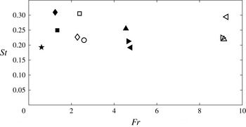
is shown in figure 10, and varies between 0.2 and 0.3, with an average
 $\mathit{St}\approx 0.24$
. If
 $\mathit{St}$
is computed by
 $\mathit{St}=kR$
, the resulting range
 $\mathit{St}\in [0.9,1.7]$
agrees well with the similar measure reported by Chomaz et al. (Reference Chomaz, Bonetton and Hopfinger1993) for the homogeneous sphere wake in this
 $\mathit{Re}$
range. However, there is no obvious dependence on either
 $\mathit{Re}$
or
 $\mathit{Fr}$
, in contrast with the
 $\mathit{Re}^{0.5}$
dependence for the sphere, perhaps because the grid shear layer does not start from a growing boundary layer, but always begins abruptly at the same corner point.
Strouhal number of the wake-edge vortices. The symbols correspond to the cases listed in table 1.

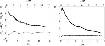
Initially wake-edge vortices merge with neighbours (figure 3), growing in size but decaying in intensity. The early-time mean vorticity has two primary sources: the vertical shear due to the streamwise velocity gradient, and the horizontal shear due to the lee wave. The mean lateral vorticity
 $\overline{{\it\omega}}_{y}$
, the horizontal shear
 $\partial \overline{w}/\partial x$
and the vertical shear
 $\partial \overline{u}/\partial z$
are shown in figure 11 for
 $\mathit{Fr}=0.6$
and 9.0. In the early wake, though
 $\overline{w}$
is about the same magnitude as
 $\overline{u}$
(evident in figures 7 and 9), the horizontal shear is much smaller than the vertical shear. Even at low
 $\mathit{Fr}=0.6$
, when the early vertical motion is expected to be vigorous, the vertical shear
 $\partial \overline{u}/\partial z$
still predominates and accounts for most
 $\overline{w}_{y}$
at late times, when vertical motion is suppressed. For high
 $\mathit{Fr}$
,
 $\overline{w}$
is initially small, and
 $\partial \overline{u}/\partial z$
remains a close measure of
 $\overline{{\it\omega}}_{y}$
(figure 11
b). This implies that the decay of
 $\overline{{\it\omega}}_{y}$
at the wake edge is not strongly influenced by
 $\mathit{Fr}$
even at early times.
Horizontal vorticity
 $\overline{{\it\omega}}_{y}$
(solid line), vertical shear
 $-\partial \overline{u}/\partial z$
(dashed line) and horizontal shear
 $\partial \overline{w}/\partial x$
(dotted line) for (a) R2F.6 (
 $\bigstar$
) and (b) R11F9 (▹).

To investigate the effect of
 $\mathit{Fr}$
and
 $\mathit{Re}$
on the decay of wake-edge vorticity, an appropriate scaling is sought. Because the major source of
 $\overline{{\it\omega}}_{y}$
is the vertical shear, it should be non-dimensionalized by
 $U/R$
. However, unlike the well-studied late wake of a sphere, where the velocity distribution is Gaussian, the early wake of the grid is not fully developed (see figure 5
c,d). Therefore the global length scale
 $R$
does not properly represent the length scale of the vortices themselves, which only occupy the edge of the wake, and the tow speed
 $U$
does not represent the characteristic shearing velocity. Instead, one can define a modified local vorticity thickness
 ${\it\delta}_{{\it\omega}}$
for this shear-layer problem, as the distance between the nearest two locations where
 $\overline{{\it\omega}}_{y}=0.2\overline{{\it\omega}}_{y,peak}$
, and one may also define a shearing velocity
 $\overline{u}_{s}$
as the difference between the streamwise velocities at those two locations. Taking the first available
 ${\it\delta}_{{\it\omega}}$
and
 $\overline{u}_{s}$
as the initial scales,
 $\overline{{\it\omega}}_{y}$
may be scaled by
 $\overline{u}_{s}/{\it\delta}_{{\it\omega}}$
.
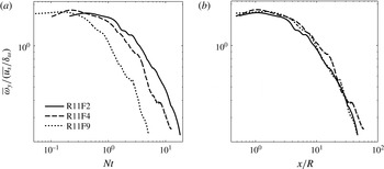
The rescaled mean vorticity is plotted against
 $Nt$
and
 $x/R$
for
 $\mathit{Re}=11\,000$
and varying
 $\mathit{Fr}$
in figure 12. For low
 $\mathit{Fr}$
, more buoyancy periods are required for the rescaled vorticity to reach the same amplitude, compared with the high-
 $\mathit{Fr}$
case. This is counter-intuitive if one imagines buoyancy to play an important role in damping
 $\overline{{\it\omega}}_{y}$
by suppressing vertical motion. When
 $\overline{{\it\omega}}_{y}$
is plotted against
 $x/R$
, the curves collapse fairly well (figure 12
b), regardless of
 $\mathit{Fr}$
. The observation is on the mean vorticity, and
 $\mathit{Fr}$
could still affect the vertical shear through fluctuating quantities and through
 $\partial \overline{v}/\partial z$
. This possible influence on the flow instability will be discussed further in the following two sections.
Rescaled vorticity decay at the wake edge for
 $\mathit{Re}=11\,000$
: (a) against
 $Nt$
; and (b) against
 $x/R$
.

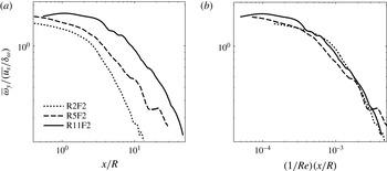
The effect of
 $\mathit{Re}$
is shown in figure 13(a) for
 $\mathit{Fr}=2.4$
. It can be seen that
 $\overline{{\it\omega}}_{y}$
decays more slowly at higher
 $\mathit{Re}$
because viscous forces weaken compared with inertia-related forces as
 $\mathit{Re}$
increases. A simple
 $\mathit{Re}^{-1}$
scaling as shown in figure 13(b) collapses the curves quite well.
Rescaled vorticity decay at the wake edge for
 $\mathit{Fr}=2.4$
: (a) against
 $x/R$
; and (b) against
 $(1/\mathit{Re})(x/R)$
.

Once a vertical structure is set, then the ensuing vertical gradients of the horizontal velocity slow down primarily by viscosity. The strong influence of viscosity and comparative unimportance of stratification parameters is quite consistent with the expected phenomenology in a strongly stratified regime with low buoyancy Reynolds number. It is this regime to which most previous laboratory experiments on strongly stratified turbulence gravitate (Fincham et al. Reference Fincham, Maxworthy and Spedding1996; Spedding Reference Spedding1997; Praud et al. Reference Praud, Fincham and Sommeria2005). The estimation of local buoyancy Reynolds number is considered later.
3.2.3. The magnitude and scaling of shear components
The importance of
 $\overline{(\partial u/\partial z)^{2}}$
in determining the kinetic energy dissipation is consistent with grid turbulence experiments by Fincham et al. (Reference Fincham, Maxworthy and Spedding1996) and Praud et al. (Reference Praud, Fincham and Sommeria2005). There is a closer resemblance to the sphere wakes of Spedding (Reference Spedding2002) because of the influence of the mean flow, which breaks the expected rough equivalence of
 $\overline{(\partial u/\partial z)^{2}}$
with
 $\overline{(\partial v/\partial z)^{2}}$
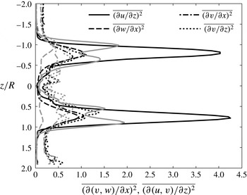
. Figure 14 shows selected shear components available in the experiments at
 $Nt=5$
and
 $Nt=10$
. Though
 $\overline{(\partial u/\partial z)^{2}}\gg \overline{(\partial v/\partial z)^{2}}$
at early times, the difference between them decreases.
Shear components in vertical slices, for
 $\mathit{Fr}=1.3$
and
 $\mathit{Re}=2700$
(R2F1, ♦). The black and grey lines show
 $Nt=5$
and 10, respectively. Solid, dashed, dash-dotted and dotted lines show
 $\overline{(\partial u/\partial z)^{2}}$
,
 $\overline{(\partial w/\partial x)^{2}}$
,
 $\overline{(\partial v/\partial x)^{2}}$
and
 $\overline{(\partial v/\partial z)^{2}}$
, respectively.

It is expected that
 $\overline{(\partial w/\partial x)^{2}}$
be much smaller than
 $\overline{(\partial v/\partial x)^{2}}$
(Spedding Reference Spedding2002) since the stratification suppresses the horizontal gradient of vertical velocity, but, owing to the lee-wave-generated mean flow,
 $\overline{(\partial w/\partial x)^{2}}$
is similar in magnitude to
 $\overline{(\partial v/\partial x)^{2}}$
at early times, becoming smaller as the amplitude of the lee wave decreases in the far wake.
The strong vertical shear is thought to be an important mechanism for triggering secondary turbulence (Lilly Reference Lilly1983; Hebert & de Bruyn Kops Reference Hebert and de Bruyn Kops2006a
), even in strongly stratified flows (Riley & de Bruyn Kops Reference Riley and de Bruyn Kops2003; Diamessis et al.
Reference Diamessis, Spedding and Domaradzki2011), and therefore has received significant attention in the literature. The averaged mean-squared vertical shear
 $S^{2}$
is
 $$\begin{eqnarray}S^{2}=\overline{\left(\frac{\partial u}{\partial z}\right)^{2}}+\overline{\left(\frac{\partial v}{\partial z}\right)^{2}}.\end{eqnarray}$$
As
 $\overline{(\partial u/\partial z)^{2}}$
dominates, non-negligible
 $S^{2}$
occurs primarily at the wake edge where the most vigorous KH modes occur, and here, as we have already seen, both the geometry and location of these layers are strongly influenced by the lee waves. The evolution of
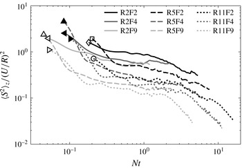
 $\langle S^{2}\rangle _{z}/(U/R)^{2}$
(
 $\langle \cdots \rangle _{z}$
is a temporal average and the value over the wake region between
 $[-L_{z},L_{z}]$
) is shown in figure 15. Note that, since the mean vertical shear is taken over the entire wake region, the global length,
 $R$
, and velocity,
 $U$
, scales are used.
Evolution of non-dimensional mean-square vertical shear integrated vertically over the wake region. Solid, dashed and dotted lines denote
 $\mathit{Re}=2700$
, 5700 and 11 000, respectively. Black, dark grey and light grey lines denote
 $\mathit{Fr}=\{2.4,4.7,9.1\}$
, respectively. A symbol is added to the beginning of each line for further clarity.

At fixed
 $\mathit{Re}$
, increasing
 $\mathit{Fr}$
leads to lower
 $\langle S^{2}\rangle _{z}/(U/R)^{2}$
, as expected. In Spedding (Reference Spedding2002) the
 $\mathit{Fr}$
dependence of
 $\overline{(\partial u/\partial z)^{2}}$
was removed when only fluctuating
 $u$
components were included. However, at fixed
 $\mathit{Fr}$
, higher
 $\mathit{Re}$
is also associated with a smaller
 $\langle S^{2}\rangle _{z}/(U/R)^{2}$
. For this particular experiment, this means that at the same
 $Nt$
(or, equivalently, same
 $x/R$
, since
 $\mathit{Fr}$
is fixed), though the towing speed is doubled from case to case, the average vertical shear is increased by a multiplier less than 2. The consequences of this will be discussed later.
Diamessis et al. (Reference Diamessis, Spedding and Domaradzki2011) found that a scaling of
 $[\langle S^{2}\rangle /(U/R)^{2}](\mathit{Fr}^{2}/\mathit{Re})$
, where
 $\langle \cdots \rangle$
denotes averaging over the volume of the wake, collapsed the late-wake data for
 $30<Nt<200$
. The
 $\mathit{Re}$
contribution comes from arguments in Riley & de Bruyn Kops (Reference Riley and de Bruyn Kops2003), who suggested that
 $[\langle S^{2}\rangle /(U/R)^{2}]/\mathit{Re}$
, which is a part of the full dissipation term, would be independent of
 $\mathit{Re}$
once truly turbulent-like behaviour is developed. Noting the differences above in how
 $\mathit{Re}$
and
 $\mathit{Fr}$
are varied, the same rescaling fails to collapse
 $\langle S^{2}\rangle _{z}$
(mean vertical shear over the vertical centreplane only) here. However, in the early wake of a grid, the velocity profile is not fully developed and not Gaussian-like, and the global scales of
 $R$
and
 $U$
may not be the best scaling parameter for
 $\langle S^{2}\rangle$
. Regardless of non-dimensionalization, a scaling of
 $\mathit{Re}^{-1}$
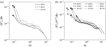
collapses the dimensional shear with moderate success in figure 16(a). If
 $\mathit{Fr}$
is varied systematically, then
 $\mathit{Fr}^{-2}$
overcompensates in early wakes. Arguing that a late-wake,
 $\mathit{Fr}$
-independent state has not yet been reached, one may empirically search for a different scaling for
 $\mathit{Fr}$
, as shown in figure 16(b), a result that is purely empirical, and may depend on this particular grid geometry. We return to this point later.
Vertically averaged mean-square vertical shear: (a) rescaled with
 $1/\mathit{Re}$
, against
 $Nt$
, for
 $\mathit{Fr}=4.7$
, and (b) rescaled with
 $\mathit{Fr}^{0.7}/\mathit{Re}$
, against
 $Nt$
, for the same dataset as figure 15.

3.2.4. Flow instability and stratified turbulence
The strength of the vertical shear and its likely role in promoting local overturning instability can be measured by a minimum Richardson-number criterion. The local Richardson number,
 $\mathit{Ri}_{loc}$
, is
 $$\begin{eqnarray}\mathit{Ri}_{loc}=\frac{N^{2}}{S^{2}}.\end{eqnarray}$$
Richardson number
 $\mathit{Ri}_{loc}$
is more of a semi-local number because
 $S$
has a local value, varying across the wake, while
 $N$
is just the global
 $N$
. This is an enforced simplification because there are no data on local
 ${\it\rho}(x,z)$
, or its spatial gradients. In practice, one may expect quite strong initial variations in
 ${\it\rho}(x,z)$
in a turbulent stratified wake (Xu, Fernando & Boyer Reference Xu, Fernando and Boyer1995). With the resulting wide variation in local
 $N$
, it might be hard in any event to compute a meaningful
 $\mathit{Ri}_{loc}$
. Doing so in this experiment must await planned density profile measurements.
At any given
 $Nt$
, since
 $N$
is constant,
 $\mathit{Ri}_{loc,min}$
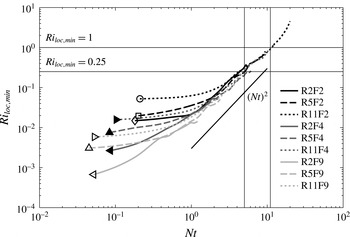
will occur at the wake edge. Its time evolution is given in figure 17. All cases begin at a value much smaller than the nominal critical value of
 $1/4$
. The initial values have a systematic dependence on both
 $\mathit{Fr}$
and
 $\mathit{Re}$
. For cases of the same
 $\mathit{Re}$
, the smaller the
 $\mathit{Fr}$
, the larger the initial
 $\mathit{Ri}_{loc,min}$
, meaning that vertical overturning is more suppressed in the beginning. This dependence is the same as reported by Diamessis et al. (Reference Diamessis, Spedding and Domaradzki2011). For
 $\mathit{Fr}$
fixed, larger
 $\mathit{Re}$
corresponds to larger initial
 $\mathit{Ri}_{loc,min}$
, perhaps counter-intuitively, and in contrast with the simulations.
Local minimum Richardson number, against
 $Nt$
, for the same dataset as figure 15.

After the initial gradual increase, the further increase in
 $\mathit{Ri}_{loc,min}$
is
 $\mathit{Fr}$
-independent and scales as
 $(Nt)^{2}$
. For smaller
 $\mathit{Fr}$
, this late-time limit is reached at a relatively larger
 $Nt$
. The same
 $\mathit{Fr}$
independence was also observed by Spedding (Reference Spedding2002) and Diamessis et al. (Reference Diamessis, Spedding and Domaradzki2011) for the wake of a sphere. Though
 $\mathit{Re}$
independence is also observed here, the contrasting
 $\mathit{Re}$
dependence is observed in Diamessis et al. (Reference Diamessis, Spedding and Domaradzki2011) when
 ${\it\nu}$
is changed, and we can only claim
 $\mathit{Re}$
independence for
 ${\it\nu}$
fixed.
In figure 17,
 $\mathit{Ri}_{loc,min}$
crosses unity at
 $Nt\approx 10$
for all conditions. This value is the same as that reported by Diamessis et al. (Reference Diamessis, Spedding and Domaradzki2011) for the low
 $\mathit{Re}=5000$
runs. The criterion of
 $\mathit{Ri}_{loc}<1$
for development of shear instability, and therefore stratified turbulence, may be argued to be equivalent to
 $\mathit{Re}_{H}\mathit{Fr}_{H}^{2}>1$
(Riley & de Bruyn Kops Reference Riley and de Bruyn Kops2003; Hebert & de Bruyn Kops Reference Hebert and de Bruyn Kops2006a
,Reference Hebert and de Bruyn Kops
b
), where
 $\mathit{Re}_{H}=u_{H}l_{H}/{\it\nu}$
is the horizontal Reynolds number and
 $\mathit{Fr}=u_{H}/(l_{H}N)$
is the horizontal Froude number.
If correctly defined on local fluctuating quantities,
 $\mathit{Re}_{H}\mathit{Fr}_{H}^{2}$
is also a close estimation of the buoyancy Reynolds number
 $\mathit{Re}_{b}$
. Here,
 $u_{H}$
is defined as the average of
 $u^{\prime }$
at the wake top edge and bottom edge, and
 $l_{H}$
represents the horizontal length scale of local overturning, and is therefore computed from the zero-crossing of the autocorrelation functions of fluctuating vertical velocity
 $w^{\prime }$
and vorticity
 ${\it\omega}_{y}^{\prime }$
at the wake edge. In each experiment run, for each wake edge location with the same
 $x/R$
(or equivalently
 $Nt$
),
 $w^{\prime }$
and
 ${\it\omega}_{y}^{\prime }$
can be reconstructed in a time series. Then the time difference between the first positive zero-crossing and first negative zero-crossing is computed for the autocorrelation functions of the
 $w^{\prime }$
and
 ${\it\omega}_{y}^{\prime }$
sequences separately, and denoted as
 ${\rm\Delta}t_{l1}$
and
 ${\rm\Delta}t_{l2}$
, indicating the time it takes for an overturning to pass that location. The local time scale can be written as
 ${\rm\Delta}t_{lH}=({\rm\Delta}t_{l1}+{\rm\Delta}t_{l2})/2$
. Then
 $l_{H}$
is computed from
 $l_{H}={\rm\Delta}t_{lH}\,u_{loc}$
, where
 $u_{loc}$
is the local mean horizontal velocity with respect to the grid at the wake edge. Finally, results from all runs are averaged, and the average of
 $l_{H}$
at the top edge and bottom edge is taken as the final
 $l_{H}$
. This procedure only works for the early wake when the wake edge definition is valid and the vertical motion has not been completely suppressed.
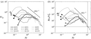
Figure 18 shows the evolution of
 $\mathit{Fr}_{H}$
and
 $\mathit{Re}_{H}\mathit{Fr}_{H}^{2}$
for different cases. For constant
 $\mathit{Fr}$
, the smaller
 $\mathit{Re}$
leads to a relatively larger local
 $\mathit{Fr}_{H}$
at early times, which is consistent with the analysis in § 3.2.1. The
 $\mathit{Fr}_{H}$
value drops below unity at very small
 $Nt$
for all cases, and further decrease of
 $\mathit{Fr}_{H}$
at later time scales approximately with
 $(Nt)^{-1}$
, and is
 $\mathit{Fr}$
-independent (and given
 ${\it\nu}$
fixed,
 $\mathit{Re}$
-independent). Similar collapse of data is also observed in
 $\mathit{Re}_{H}\mathit{Fr}_{H}^{2}$
, but scales approximately with
 $(Nt)^{-2}$
.
(a) Horizontal Froude number
 $\mathit{Fr}_{H}$
, and (b)
 $\mathit{Re}_{H}\mathit{Fr}_{H}^{2}$
, against
 $Nt$
, for the same dataset as figure 15.

3.2.5. Fluctuating quantities
The primary local source of turbulence is at the wake edge, where shear layers induce KH instability and eddies form. Then the eddies evolve by a pairing–merging mechanism and spread into the interior wake. In this section we examine the characteristics of the turbulent quantities.
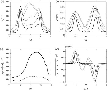
Figure 19(a,b) shows the vertical profiles of
 $u^{\prime }/U$
and
 $w^{\prime }/U$
at different
 $Nt$
for
 $\mathit{Fr}=4.7$
and
 $\mathit{Re}=5700$
. Before
 $Nt=3$
, the shape and magnitude of
 $u^{\prime }/U$
and
 $w^{\prime }/U$
are closely matched, with peak values at
 $z/h=\pm 1$
. The magnitude and width of the peaks of both
 $u^{\prime }/U$
and
 $w^{\prime }/U$
increase with
 $Nt$
. Note that the latter peaks are slightly broader in
 $z$
as waves propagate to the exterior. After
 $Nt=3$
, the maxima in
 $u^{\prime }/U$
have grown in the midline, while
 $(w^{\prime }/U)_{max}$
remains around
 $z/h=\pm 1$
. Figure 19(c) shows the centreline
 $u_{0}^{\prime }/U$
and
 $w_{0}^{\prime }/U$
. The shapes of the two curves are perhaps similar, increasing at early times as the wake becomes more turbulent, and then dissipating due to viscosity, but the amplitudes are very different. Not only is the initial forcing not isotropic in
 $\{x,z\}$
, but wave modes propagate outwards, away from the centreline.
Fluctuating quantities for
 $\mathit{Fr}=4.7$
and
 $\mathit{Re}=5700$
(R5F4, ▴): (a)
 $u^{\prime }/U$
in vertical slices; (b)
 $w^{\prime }/U$
in vertical slices; (c)
 $u_{0}^{\prime }/U$
(solid line) and
 $w_{0}^{\prime }/U$
(dashed line) in wake centre; and (d) Reynolds stress in vertical slices. In panels (a), (b) and (d),
 $z$
is non-dimensionalized by the local wake half-height. Black solid line, black dashed line and black dotted line are for
 $Nt=\{1,2,3\}$
, respectively; grey solid line and grey dashed line are for
 $Nt=\{4,6\}$
.

The Reynolds stress in vertical slices is plotted in figure 19(d) for the same case. The peak values are located around
 $z/h=\pm 1$
, with magnitude increasing before
 $Nt=3$
, and decreasing after
 $Nt=4$
. The inner wake region becomes quite turbulent after
 $Nt=4$
as another opposite-sign peak occurs between the wake edge and centre, and grows even larger in magnitude than the wake edge peak at
 $Nt=6$
.
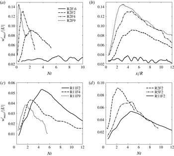
At early times, the fluctuating quantities reflect the simultaneous dynamics of KH modes with the lee wave at the wake edge. Figure 20(a) shows the maximum fluctuating vertical velocity against
 $Nt$
for
 $\mathit{Re}=2700$
but varying
 $\mathit{Fr}$
. As
 $\mathit{Fr}$
increases, so does
 $w_{max}^{\prime }$
and the peak occurs at smaller
 $Nt$
. When
 $\mathit{Fr}=(1/N)/(R/U)$
is high,
 $R/U$
is small compared with
 $1/N$
, and a maximum after a fixed number of overturns appears at smaller
 $Nt$
. If plotted against
 $x/R$
, the maxima occur at
 $x/R\in [3,5]$
as shown in figure 20(b).
Plots of
 $w_{max}^{\prime }/|U|$
in the wake region for: (a) constant
 $\mathit{Re}=2700$
, varying
 $\mathit{Fr}$
, against
 $Nt$
; (b) same data as (a), but against
 $x/R$
; (c) constant
 $\mathit{Re}=11\,000$
, varying
 $\mathit{Fr}$
, against
 $Nt$
; and (d) constant
 $\mathit{Fr}=2.4$
, varying
 $\mathit{Re}$
, against
 $Nt$
.

At higher
 $\mathit{Re}$
, the trend that
 $w_{max}^{\prime }$
peaks at smaller
 $Nt$
for larger
 $\mathit{Fr}$
persists but the amplitude does not increase systematically. Here
 $\mathit{Re}$
may be large enough so that initial turbulent dissipation has removed kinetic energy from the eddy motions before there is any significant interaction with the exterior. If that is so, then it presumably contrasts with low-
 $\mathit{Re}$
cases where this does not happen, and figure 20(a,c) has results from the same physical experiment, but in two rather different dynamical regimes, distinguished by
 $\mathit{Re}_{H}\,\mathit{Fr}_{H}^{2}=\mathit{Re}_{b}$
.
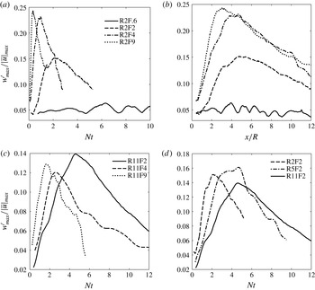
Because
 $\mathit{Re}_{H}\,\mathit{Fr}_{H}^{2}$
is a local parameter, to be consistent,
 $w_{max}^{\prime }$
is non-dimensionalized by the maximum
 $|\overline{u}|$
at the wake edge behind the grid, which occurs at
 $Nt$
roughly equal to that of the initial dip in figure 9. The results for similar cases are shown in figure 21. The peak locations and magnitudes match reasonably well with those shown in figure 18(b). For
 $\mathit{Re}=2700$
,
 $\mathit{Fr}=9.1$
and
 $\mathit{Fr}=4.7$
have
 $\mathit{Re}_{b,max}>200$
,
 $\mathit{Fr}=2.4$
has
 $\mathit{Re}_{b,max}\approx 30$
, and
 $\mathit{Fr}=0.6$
has
 $\mathit{Re}_{b,max}$
below unity, so the peak magnitudes of
 $w_{max}^{\prime }/|\overline{u}|_{max}$
differ considerably. The three cases with
 $\mathit{Re}=11\,000$
have
 $\mathit{Re}_{b,max}\in [20,100]$
, and the three cases with
 $\mathit{Fr}=2.4$
have
 $\mathit{Re}_{b,max}\in [10,30]$
, indicating that they are probably in the same dynamical regime, respectively, so peak magnitudes of
 $w_{max}^{\prime }/|\overline{u}|_{max}$
are similar.
Plots of
 $w_{max}^{\prime }/|\overline{u}|_{max}$
in the wake region, where
 $|\overline{u}|_{max}$
is the maximum mean streamwise velocity at the wake edge behind the grid, for the same dataset as figure 20.

4. Discussion
4.1. Initial conditions in stratified wakes
As noted in the introduction, independently, for stratified experiments in general (§ 1.2), for simulations in boxes (§ 1.3) and for both types of investigations of localized stratified turbulence (§ 1.4), there has been continuing discussion on the generality of any given configuration. Even when turbulent stratified wakes can be shown to be indistinguishable at late times, given a proper rescaling by the initial horizontal momentum flux (Meunier & Spedding Reference Meunier and Spedding2004), the conjectured similarity at early times has not been demonstrated, only inferred. Here, detailed examination of one particular case is sufficient to show that there cannot be a universal or general set of initial conditions. In figure 8, the lee wavelength,
 ${\it\lambda}$
, agrees satisfactorily with previous experiments, both laboratory and numerical, on a sphere wake. The variation of wave amplitude with Fr, however, is quite different, and is because of the varying (and sometimes counter-intuitive) influence of Fr and Re on the effective grid obstruction itself. This is only one case, but it is sufficient to dismiss a general claim.
4.2. Initial three-dimensional turbulence?
The experiment and analysis methods described here were deliberately configured to allow measurements at early times, close to the grid. Figure 4 shows how instantaneous and mean data are available at
 $x/R<1/2$
and
 $Nt<1/2$
, limited only by the stereoscopic access of the camera pair. These small
 $x/R$
are sufficient, however, to provide data at supposed 3D regimes (
 $Nt<2$
; Spedding Reference Spedding1997). The velocity field, whenever measurable, is always affected by the presence of the background density gradient. For example, in figure 9, the centreline velocity is greatly affected by the lee wave at low
 $\mathit{Fr}$
. The initial flow is not isotropic, but the peak local values of
 $w_{max}^{\prime }/|\overline{u}|_{max}$
in figure 21 also always have some systematic variation with Fr. The difference in peak values is more pronounced at low Re, and at high Re one might claim some general similarity for
 $Nt<2$
. There is no truly 3D turbulent field in this experiment. If there is a minimum Fr required for some effectively unstratified early motion, then it must be at least
 $\mathit{Fr}>9$
, the maximum tested.
4.3. Buoyancy Reynolds number in laboratory experiments
A condition for true turbulence in the presence of stratification is often set on
 $\mathit{Re}_{H}\mathit{Fr}_{H}^{2}$
. If
 $\mathit{Re}_{H}\mathit{Fr}_{H}^{2}$
is equivalent to buoyancy Reynolds number (Hebert & de Bruyn Kops Reference Hebert and de Bruyn Kops2006a
), then the late-time scale separation between the Ozmidov and Kolmogorov scales is also independent of
 $\mathit{Fr}$
. In figure 18(b), the experimentally derived
 $\mathit{Re}_{H}\mathit{Fr}_{H}^{2}$
cross unity at
 $Nt\approx 10$
for all cases. This agrees with the result in
 $\mathit{Ri}_{loc,min}$
(figure 17), supporting the idea of their equivalence in predicting/measuring stratified turbulence. Before
 $Nt\approx 10$
, because
 $\mathit{Fr}_{H}<1$
and
 $\mathit{Re}_{H}\mathit{Fr}_{H}^{2}>1$
, the flow in this experiment can be asserted to be mostly in the ‘stratified turbulence regime’ (Brethouwer et al.
Reference Brethouwer, Billant, Lindborg and Chomaz2007) and to be weakly viscous (Waite Reference Waite2013), and dissipation at large scales is negligible. After
 $Nt\approx 10$
, because
 $\mathit{Fr}_{H}<1$
and
 $\mathit{Re}_{H}\mathit{Fr}_{H}^{2}<1$
, the flow starts to enter the ‘viscous-affected stratified flow regime’, the stratified turbulence is strongly damped by viscosity, and dissipation occurs predominantly at large scales. The results of the towed grid are in good agreement with prevailing notions of a minimum
 $\mathit{Re}_{H}\mathit{Fr}_{H}^{2}$
for true turbulence in a stratified medium. As in previous experiments (Fincham et al.
Reference Fincham, Maxworthy and Spedding1996; Spedding et al.
Reference Spedding, Browand and Fincham1996b
; Praud et al.
Reference Praud, Fincham and Sommeria2005), there is a short period of time available before no range of scales for turbulence is available. Though at late times, the flow in the vertical centreplane tends to evolve in a similar way, and is viscous-stratification-dominated, the trajectory for the flow to enter such a state varies. These trajectories are not general and vary in sometimes curious ways with Re and Fr.
4.4. Parametrization and comparison with numerical simulation
There are a number of occasions in this study where Reynolds number dependence and parametrizations from experiment and simulation do not agree, or are not equivalent. For example, the observed
 $\mathit{Re}$
dependence of
 $\langle S^{2}\rangle _{z}/(U/R)^{2}$
in figure 15 is not the same as presented in Diamessis et al. (Reference Diamessis, Spedding and Domaradzki2011). There are two sets of considerations that are different in the experiments and in the simulations. In numerical experiment, the nominal
 $\mathit{Re}$
is varied by modifying
 ${\it\nu}$
, with
 $U$
constant, and so an
 $\mathit{Re}$
dependence of the non-dimensional shear is the same as that of the dimensional shear, which actually has the same
 $\mathit{Re}$
dependence as this experiment. Second, as previously noted in § 3.2.1, the streamwise velocity behind the grid does not preserve scale similarity, thus making the local
 $\mathit{Fr}$
and
 $\mathit{Re}$
relations different from nominal. For example, in the simulations,
 $U$
is constant and therefore
 $N$
is constant for a fixed
 $\mathit{Fr}$
, but
 $N$
in laboratory experiments scales with
 $U$
to keep
 $\mathit{Fr}$
constant. Therefore, in experiment, when
 $\mathit{Re}$
doubles,
 $N$
also doubles, but the local vertical shear is increased by a multiplier less than 2. Therefore quantities that ought to scale on
 $U$
must use a local
 $U$
, found from experiment. This value is peculiar to this experiment, and probably to this grid permeability. It is why for fixed
 $\mathit{Fr}$
, higher
 $\mathit{Re}$
is associated with a smaller
 $\langle S^{2}\rangle _{z}/(U/R)^{2}$
, and it is why
 $\mathit{Ri}_{loc,min}$
apparently increases for larger
 $\mathit{Re}$
.
Doubling Re or Fr may thus not be equivalent in laboratory or numerical experiment, because each is making transitions between dynamically different regimes at different points. Dynamical equivalence is only assured for geometrically similar flows, and the local geometry of the grid forcing here is not the same as the wake behind a sphere, or for turbulence superimposed on a mean profile.
5. Conclusions
The turbulent wake of a grid was studied partly as a means of generating turbulence of varying intensity to observe the interaction with the stable density background, and partly as a means of producing a patch of turbulence free to evolve in space and time. At the same time, one may look for similarities and differences with the much-studied sphere wake.
In the absence of evidence to the contrary – in fact, in the absence of any evidence at all from near-wake turbulence in stratified fluids – it has been conjectured (e.g. Spedding Reference Spedding1997) that there is an initial stage in stratified wakes where the flow evolves much as it does in the absence of stratification. General and universal models have even been proposed for all wake defect magnitudes and signs provided they are not very close to zero (the momentumless condition) (Meunier & Spedding Reference Meunier and Spedding2004, Reference Meunier and Spedding2006), and simple analytical models have been constructed starting with this base condition over a wide range of
 $\mathit{Re}$
and
 $\mathit{Fr}$
(Meunier, Diamessis & Spedding Reference Meunier, Diamessis and Spedding2006). The results presented here show that there can be no such universal initial condition. For
 $\mathit{Fr}\in \{0.6,10\}$
and
 $\mathit{Re}\in \{2700,11\,000\}$
there are no conditions where the flow can be claimed to be either 3D or universal.
There is an interesting interplay between the dynamics of lee-wave motions and of shear-layer instabilities. The balance between them is reasonably captured by an internal Froude number,
 $\mathit{Fr}=(1/N)(U/R)$
, where
 $1/N$
is a characteristic time scale of the lee wave and
 $R/U$
is an eddy turnover time. In fact, the shear-layer evolution can proceed almost oblivious of
 $\mathit{Fr}$
at either low or high
 $\mathit{Fr}$
, and so there are different trajectories for the flow to arrive at a late-time regime. These trajectories can be described in terms of
 $\mathit{Re}_{H}\mathit{Fr}_{H}^{2}$
, and the experiments described here cover a range where some may be claimed to be turbulent for some number of overturns, and over some range of scales, while others are constrained from the start by either stratification or viscosity, or both.
Though this is a rather detailed study of one grid geometry over a range of
 $\{\mathit{Re},\mathit{Fr}\}$
, the consistent time averaging and sampling in a reference frame attached to the body sets the stage for further studies that can compare the specific effect of various geometries on early-wake parameters, some of which emerge to set the conditions for the persistent late wakes.
Acknowledgements
We most gratefully acknowledge the support of ONR Contract N00014-14-1-0422, under the management of Dr R. Joslin. We also thank three reviewers for their very careful reading of the first version and helpful comments.