1. Introduction
For wall-bounded turbulence, the most important physical processes take place within the near-wall region which accounts for extremely high levels of turbulence production and Reynolds stresses (Vallikivi et al. Reference Vallikivi, Hultmark and Smits2015) due to the strong shear confirmed by numerous studies occurring with the presence of complex flow structures (Dennis Reference Dennis2015; Jiménez Reference Jiménez2018). However, accurate measurements and simulations of this area are always challenging owing to the exceedingly large span of fluid length scales (Adrian Reference Adrian2010), especially at extreme Reynolds numbers in the atmospheric surface layer (ASL) where a phenomenological picture of very large-scale motions coexisting and interacting with structures from the hairpin paradigm has been provided (Guala et al. Reference Guala, Metzger and McKeon2011). Therefore, the prediction of turbulence behaviour therein based on the interaction between the inner and outer regions, which caters to experiments and numerical simulations, has become a topic with considerable applied value in the field (Marusic et al. Reference Marusic, Mathis and Hutchins2010a ; Mathis et al. Reference Mathis, Marusic, Chernyshenko and Hutchins2013).
To accurately characterize the differences and correlations between the inner and outer regions and overcome the difficulty in obtaining near-wall turbulence statistics at high Reynolds numbers, Marusic et al. (Reference Marusic, Mathis and Hutchins2010a
) (MMH hereafter) proposed a predictive model using the velocity signal at the centre of the logarithmic region as the only input. They reconstructed fluctuating streamwise velocity signals near the wall by using a concise mathematical formulation under a mechanism of self-sustaining small-scales in the inner region as well as the superposition and the amplitude modulation from large-scale structures in the outer region. The MMH model was shown to have good applicability in the turbulent boundary layer (TBL) at friction Reynolds number
 $Re_{\tau }=\delta u_{\tau }/\nu$
= 2800–19 000 (where
 $\delta$
is the boundary layer thickness,
 $u_{\tau }$
is the friction velocity and
 $\nu$
is the kinematic viscosity). In this model, the self-sustaining small scales are formulated in a universal signal assumed to be independent of Reynolds number and predetermined in calibration experiments. The outer large-scale ‘footprint’ is quantified by a superposition coefficient in the linear term of the formulation, and the amplitude modulation is expressed in the quadratic nonlinear term. Mathis et al. (Reference Mathis, Hutchins and Marusic2011) generalized the model to pipe flows, channel flows and adverse pressure gradient flows, confirming the reliability of it and its potential for utility at extremely high Reynolds numbers. In addition to the classic MMH model, there are several recent studies that predict near-wall turbulence based on machine learning, such as natural visibility graph (Iacobello et al. Reference Iacobello, Ridolfi and Scarsoglio2021), convolutional neural network (Schmekel et al. Reference Schmekel, Alcántara-Ávila, Hoyas and Vinuesa2022) and generative adversarial network (Oh et al. Reference Oh, Lee, Son, Kim and Ki2022).
In the last decade, various studies have been conducted to polish the MMH model, mostly centring around the accurate capture of the interactions between scales and the representation of the universal small-scale signal. Mathis et al. (Reference Mathis, Marusic, Chernyshenko and Hutchins2013) replaced the complex calibration methods in the spirit of a quasisteady hypothesis for determining the demodulation coefficient and extended the prediction to the wall-shear stress fluctuations. Chernyshenko et al. (Reference Chernyshenko, Marusic and Mathis2012) and Zhang & Chernyshenko (Reference Zhang and Chernyshenko2016) derived theoretical expressions for the superposition and the modulation coefficients under quasisteady hypothesis in which the coefficients show correlations with the mean velocity profile and the turbulence intensity of the streamwise velocity fluctuation. Agostini & Leschziner (Reference Agostini and Leschziner2014) used the near-wall local friction velocity instead of the global one to scale the small scales and account for the asymmetric response to different large-scale events, further excluding the effect of large scales to obtain a more unaffected near-wall universal signal. Recently, spectral linear stochastic estimation (SLSE) has been applied in flow decomposition, with which the scales that are linearly coherent in two positions could be isolated (e.g. Blackman & Perret Reference Blackman and Perret2016). To assess the superposition effect, Baars et al. (Reference Baars, Hutchins and Marusic2016) investigated the large-scale coherence in the frequency domain by using linear stochastic estimation and modified the superposition coefficients in the MMH model to a scale-dependent kernel, which amended the prediction results with a refined linear term of the formulation. What is more, they noticed the time shift in the modulation and the model was upgraded in the other aspect in its modulation term.
To bypass stringent calibration experiments, many of the researches also attempted to find an alternative approach to acquire the universal signal in the MMH model. Inspired by the minimal flow unit, Yin et al. (Reference Yin, Huang and Xu2017) demonstrated its similarity to the universal signal in turbulence intensity, energy spectrum and joint probability density function (PDF) and used it as a surrogate of the small-scale part in the original model, which led to acceptable predictive results despite the unavoidable mismatch in the predicted high-order moments stemming from a periodic extended minimal flow unit. Han et al. (Reference Han, Liu, Bo and Zheng2019) and Zheng & Bo (Reference Zheng and Bo2022) employed harmony superposition method to generate the small-scale signal in accordance with the velocity power spectrum proposed by Kaimal et al. (Reference Kaimal, Wyngaard and Izumi1972), with which the complicated calibration can be omitted and the predictions suffice in engineering. But the artificial small-scale phases may lead to phase disorder in predicted results and hinder the estimation for high-order statistics.
In summary, numerous attempts have been made to modify turbulence predictive models, but one with high universality and accuracy has been absent to date, especially in terms of the prediction of high-order statistics, which depends on appropriate capture of amplitude modulation (Mathis et al. Reference Mathis, Hutchins and Marusic2011). The amplitude modulation refers to a nonlinear effect of large-scale motions in the outer region on the near-wall small scales, originally studied by Brown & Thomas (Reference Brown and Thomas1977), who observed that the amplitude of small-scale fluctuation was related to the large-scale signal. Based on the streamwise velocity fluctuations of various shear flows, Bandyopadhyay & Hussain (Reference Bandyopadhyay and Hussain1984) found a strong correlation between the low-frequency signal and the envelope of the high-frequency one, with the latter tending to lead the former by as much as half a cycle near the wall. It is now generally accepted that the amplitude modulation is most intuitively manifested as the amplitudes of the small scales would get larger or they became relatively quiescent within different large-scale fluctuations (Hutchins & Marusic Reference Hutchins and Marusic2007). Therefore, the method of quantifying the degree of amplitude modulation using the correlation coefficient between the large-scale signal and the small-scale signal envelope (Mathis et al. Reference Mathis, Hutchins and Marusic2009) is commonly accepted henceforth. Given that Duvvuri & McKeon (Reference Duvvuri and McKeon2015) explain the connection between skewness and modulation coefficient, one alternative based on the skewness profile has also emerged (Eitel-Amor et al. Reference Eitel-Amor, Örlü and Schlatter2014). Besides, it has been found that the amplitude modulation is present in both spanwise and vertical velocity fluctuations (Jacobi & McKeon Reference Jacobi and McKeon2013; Talluru et al. Reference Talluru, Baidya, Hutchins and Marusic2014), and velocity is not the only quantity that is externally modulated – so are the wall-shear stress and the pressure fluctuations (Thomas & Bull Reference Thomas and Bull1983; Abe et al. Reference Abe, Kawamura and Choi2004; Tsuji et al. Reference Tsuji, Marusic and Johansson2016).
Interestingly, phase differences (or time shifts in the time domain) between large and small scales have been observed in the amplitude modulation of velocity, shear stress and pressure, implying that changes in the amplitude of the small-scale carrier signal are not synchronized with those in the large-scale modulating signal. Chung & McKeon (Reference Chung and McKeon2010) carried out large-eddy simulation in a turbulent channel flow at
 $Re_{\tau }=2000$
and found that the phase of the large and the small scales near the wall approximately coincide, leading to a positive amplitude modulation coefficient, and that the phase difference away from the wall increases, ultimately resulting in a negative coefficient as the difference approaches
 $\pi$
, which indicates that the inclusion of the phase difference in calculating amplitude modulation coefficient enhances the understanding of the effect. Hutchins et al. (Reference Hutchins, Monty, Ganapathisubramani, H.C.H. and Marusic2011) further demonstrated that this shift in phase difference is consistent with changes in the local streamwise velocity gradient of the conditional large-scale fluctuations. Ganapathisubramani et al. (Reference Ganapathisubramani, Hutchins, Monty, Chung and Marusic2012), on the other hand, collected detailed statistics of amplitude modulation on small scales in the TBL at
 $Re_{\tau }=14150$
, confirming the phase differences between large and small scales that do not vary with the large-scale fluctuations. Baars et al. (Reference Baars, Talluru, Hutchins and Marusic2015) subsequently used the wavelet analysis to examine the variation of the time shift with height for amplitude modulation. Although time shifts in modulation have been emphasized, the few studies merely focused at moderate Reynolds numbers (Baars et al. Reference Baars, Talluru, Hutchins and Marusic2015) and lack results at high Reynolds numbers.
Another topic on amplitude modulation concerns the flow scales. The canonical decoupling procedure to calculate amplitude modulation coefficient employs a nominal cutoff wavelength
 $\delta$
to divide the fluctuating velocity into large- and small-scale components. However, a study in a high-Reynolds-number ASL by Liu et al. (Reference Liu, Wang and Zheng2019) suggested that the most energetic turbulent motions exhibit the strongest modulation effect, which shows simultaneous dependence on the local height and outer scale
 $\delta$
. For example, the large scales with the most significant contribution to amplitude modulation at the top of logarithmic region are approximately
 $\lambda _{x}\gt 10\delta$
, which is distinct from
 $\lambda _{x}\gt \delta$
in the usual sense. This is fairly easy to understand: those self-similar structures within the boundary layer (despite some others are claimed to have less similarity in geometry, (Deshpande et al. Reference Deshpande, Chandran, Monty and Marusic2020)) are hierarchical (Perry & Chong Reference Perry and Chong1982) and would self-organize and aggregate on larger scales as the distance from the wall increases and influence the near-wall cycles, implying that the modulation may be multiscale.
The nonlinear term of the MMH model reflects the amplitude modulation. However, neither the time shift nor the multiscale effect in amplitude modulation are systematically incorporated into the predictive model. On the one hand, studies on amplitude modulation at high Reynolds numbers are scarce, and few studies focused on the time shift or the multiscale effect in detail. On the other hand, these two factors have never been considered simultaneously. As Mathis et al. (Reference Mathis, Hutchins and Marusic2011) declared, the universal signals built therein are not perfect and thus retain some small amount of large-scale information. An ideal universal signal refers to one that is purely innocent of any large-scale influence, so careful inspection of the amplitude modulation exerted by large scales on it are called for, being one of the motivations on improvements of the existing predictive model. In statistics, the relative error of the models provided in Mathis et al. (Reference Mathis, Hutchins and Marusic2011) and Baars et al. (Reference Baars, Talluru, Hutchins and Marusic2015) can reach 8 % (at
 $Re_{\tau } \sim 10^{4}$
) and 34 % (at
 $Re_{\tau } \sim 10^{6}$
compared with theoretical formulations), respectively. In these scenarios, the time shift and the multiscale effect have failed to be coupled. Since the amplitude modulation is remarkably prominent in high-Reynolds-number flows, the omission of any element related to it would dim the hopes of comprehending suchan effect. Moreover, the parameters in the predictive model are calibrated from two-point simultaneous measurements at
 $Re_{\tau }\sim O(10^{3}-10^{4})$
, but extensions of these parameters to higher Reynolds numbers are limited by the lack of statistics there in. Mathis et al. (Reference Mathis, Hutchins and Marusic2011) noted the need to complement the model with refined and accurate calibration measurements at extremely high Reynolds numbers. Therefore, this study conducts the calibration experiments at
 $Re_{\tau }\sim O(10^{6})$
with the multipoint simultaneous measurements flow field data collected from long-term observations in the ASL. Furthermore, the role of the nonlinear term of the model in the prediction is emphasized and the necessity of attending the multiscale effect and the time shift in quantifying amplitude modulation is exemplified by the improvement of predictive results. The two factors are thus simultaneously considered, aiming to precisely capture the amplitude modulation at each height, which sheds light on a refined predictive scheme profiting from a delicate characterization of amplitude modulation.
2. Experimental set-up
The ASL is a truly high-Reynolds-number facility representing some of the highest Reynolds number conditions that can be achieved terrestrially, and a near-neutrally stratified ASL with steady wind can be used for the study of canonical zero-pressure-gradient TBLs after the careful specific selection and preprocessing (Marusic et al. Reference Marusic, McKeon, Monkewitz, Nagib, Smits and Sreenivasan2010b
). All data in this study were collected from the Qingtu Lake Observation Array (QLOA) in western China, which is located on the dry bed of the Qingtu Lake between the Badain Jaran Desert and the Tengger Desert (
 $103^{\circ }40'03''$
E,
 $39^{\circ }12'27''$
N). The reasons for the selection of this site are as follows: (i) the terrain is flat, and the condition of the surface is not complex, providing a flow geometry comparable to TBL on a flat plate; (ii) the monsoon-type climate ensures steady flows and high Reynolds numbers owing to prevailing north-westerly winds; (iii) frequent sandstorms also contribute to measurements of particle concentration and electric field during the occurrence of windblown sand flows, which enhance the knowledge of blown-sand physics, albeit not covered in this paper.
The QLOA consists of three-dimensional (streamwise, spanwise and vertical) observation arrays along the prevailing wind direction, with which multipoint synchronized measurements of velocities, air temperatures and other quantities concerning wind-blown particles can be realized spanning 240 m, 60 m and 30 m in the streamwise, spanwise and vertical directions. The arrays are exquisitely arranged to effectively eliminate the influence on flow fields, and the site is a unique facility that accomplishes three-dimensional multipoint simultaneous measurements of particle-free and particle-laden flows in the ASL. The QLOA has provided more than 8400 hr of continuous measurements, including wind speed, particle concentration, temperature, humidity and electric field. This study mainly centres on the data collected from the vertical high tower that consists of 11 logarithmically distributed heights, notated from low to high as follows: ht1 = 0.9 m, ht2 = 1.71 m, ht3 = 2.5 m, ht4 = 3.5 m, ht5 = 5 m, ht6 = 7.15 m, ht7 = 8.5 m, ht8 = 10.24 m, ht9 = 14.65 m, ht10 = 20.96 m and ht11 = 30 m. The wind speed and temperature are recorded by a three-dimensional sonic anemometer (CSAT3B, Campbell Scientific, Inc.) at a sample frequency of 50 Hz, which is much higher than that in Hutchins et al. (Reference Hutchins, Chauhan, Marusic, Monty and Klewicki2012). Large scales dominate these statistics at atmospheric Reynolds numbers such that the sonics can accurately capture overall (co)variances. However, inevitably, they still may be misrepresenting the small scales. More detailed information about the site and the arrangements can be found in Wang & Zheng (Reference Wang and Zheng2016).
Due to the complexity and uncontrollability of the field observations, proper pretreatments should be performed on raw data including wind direction adjustment (Wilczak et al. Reference Wilczak, Oncley and Stage2001), stratification stability judgment, quality verification (Foken et al. Reference Foken, Gockede, Mauder, Mahrt, Amiro, Munger, Lee, Massman and Law2004) and long-term detrending (Hutchins et al. Reference Hutchins, Chauhan, Marusic, Monty and Klewicki2012). After that, the data are segmented into series with a time length of 1 hr for subsequent analysis to ensure convergence (Wyngaard Reference Wyngaard1992). The pretreatments and selection criteria applied in the study are consistent with those described in Hutchins et al. (Reference Hutchins, Chauhan, Marusic, Monty and Klewicki2012) and Wang & Zheng (Reference Wang and Zheng2016). In particular, the Monin–Obukhov parameter
 $z/L$
is used for stratification stability judgment, which is defined as
 \begin{equation} z/L=-\frac {\kappa gz\overline {w'\theta '}}{U_{\tau }^3\overline {\theta }}, \end{equation}
where
 $\kappa = 0.41$
is the Kármán constant;
 $U_{\tau }$
is the friction velocity, which is obtained by least-square fitting of the mean streamwise velocity (Bagnold Reference Bagnold1941; Clauser Reference Clauser1956); g is the gravitational acceleration;
 $\overline {w^{\prime }\theta ^{\prime }}$
is the average vertical heat flux;
 $\overline {\theta }$
is the corresponding average surface temperature. In addition, the kinematic viscosity
 $\nu$
is calculated according to the air pressure and temperature of the experimental site (Tracy et al. Reference Tracy, Welch and Porter1980). Furthermore, as buoyancy and stratification can become important at positions farther away from the wall even when the
 $z/\Lambda$
values from measurements closer to the surface indicate near-neutral shear-dominated conditions,
 $z/\Lambda$
is also estimated here, where
 $\Lambda$
is the Obukhov length computed from local fluxes rather than surface (Nieuwstadt Reference Nieuwstadt1984). The data used in this study were proved satisfactory in two ways of testing. The estimation of ASL thickness
 $\delta$
is aligned with Marusic et al. (Reference Marusic, Monty, Hultmark and Smits2013) and detailed in Wang & Zheng (Reference Wang and Zheng2016).
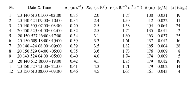
Based on the processes mentioned above, 12 sets of high-quality data
 $(Re_{\tau }=(2.0-4.5)\times 10^{6})$
in near-neutrally stratified ASL
 $(|z/L|\lt 0.1)$
are selected herein for study, with the specific information exhibited in table 1. The validity and the comparability to zero-pressure-gradient TBL statistics of the data are scrutinized theoretically and experimentally in Wang & Zheng (Reference Wang and Zheng2016) and Liu et al. (Reference Liu, Bo and Liang2017), including examinations on the mean velocity, turbulence intensity and Reynolds shear stress. The data have been applied in recent researches on length scales, structure inclination, amplitude modulation and scaling laws for statistics of coherent structures.
Informative introduction on the 12 datasets used in this paper, sorted by Reynolds number magnitude.

3. Role of the amplitude-modulation-related term
To improve the characterization of the superposition effect, Baars et al. (Reference Baars, Hutchins and Marusic2016) refined the MMH model based on the SLSE. In recent decades, stochastic estimation techniques have been widely used in turbulent flows to examine coherent structures (Adrian & Moin Reference Adrian and Moin1988; Bonnet et al. Reference Bonnet1998), while the linear stochastic estimation, which is in the simplest form, can be applied to characterize the linear transfer of energy that accounts for the large-scale ‘footprint’. The expression of this refined scheme is shown as
 \begin{equation} u_{p}^{+}(z^{+},t^{+}) = u^{*+}(z^{+},t^{+}) + \Gamma (z^{+})u^{*+}(z^{+},t^{+})u_{S}^{+}(z^{+},t^{+}-\tau _{a}^{+}) + u_{S}^{+}(z^{+},t^{+}), \end{equation}
where
 $\Gamma$
is the coefficient derived from the demodulation in the model calibration that follows Baars et al. (Reference Baars, Hutchins and Marusic2016), due to which the coefficient is called the demodulation coefficient hereafter. Essentially, the principal difference between the model refined by Baars et al. (Reference Baars, Hutchins and Marusic2016) and the MMH model are in the linear superposition term, and the inclusion of the time shift in the modulation-related term. In detail, the original footprint
 $\alpha u_{OL}^{+}$
was replaced with
 $u_{S}^{+}$
, and it has also been accordingly done in the nonlinear modulation term. In this study, the nonlinear modulation-related term is further discussed based on the scheme. Before that, the role of this term played in the demodulation for obtaining model parameters and the prediction is clarified to show the desire for subsequent refinement. In the model, the amplitude modulation on universal signal
 $u^{*+}$
(
 $u^{*}$
is part of the local signal where the modulation coefficient is 0 under large-scale motions, and details can be seen in Mathis et al. Reference Mathis, Hutchins and Marusic2011) exerted by ‘footprint’
 $u_{S}^{+}$
is fully explained in the nonlinear term
 $\Gamma u^{*+}u_{S}^{+}$
, which may affect the prediction in two aspects. In one, the extraction of
 $u^{*+}$
from the detrended signal
 $u_{d}^{+}$
(
 $u_{d}$
stands for the local signal with the footprint removed, and the access to it is detailed in Mathis et al. Reference Mathis, Hutchins and Marusic2011and Baars et al. Reference Baars, Hutchins and Marusic2016) relies on a proper quantification of amplitude modulation, otherwise the large-scale irrelevance of
 $u^{*+}$
perishes and thus inapplicable to the subsequent prediction. In the other, an inappropriate composition of the nonlinear term in predictive signals would also bring a deviation of it from actual results, which is more transparent.
Time series of fluctuating velocity at
 $z$
= 0.9 m, ASL,
 $Re_{\tau }=3.3\times 10^{6}$
. (a) Original signal
 $u$
(black line) and predictive ‘footprint’
 $u_{S}$
(red line), with colour blocks indicating the two time periods when
 $u_{S}$
pulsation is positive/negative; (b) detrending signal
 $u_{d}$
; (c) intrinsic signal
 $u^{*}$
; (d) the energy difference between
 $u_{d}$
and
 $u^{*}$
, denoted by
 $(u_{d})^{2}-(u^{*})^{2}$
, with the red line denoting
 $u_{S}$
.

Premultiplied time-frequency spectra map of streamwise velocity fluctuations
 $k_{x} \hat {\phi }_{uu}/u_{\tau }^{2}$
at
 $Re_{\tau } = 3.3 \times 10^{6}$
: (a)–(c)
 $u^{+}$
,
 $u_{d}^{+}$
and
 $u^{*+}$
; and (d) difference between spectra of
 $u_{d}^{+}$
and
 $u^{*+}$
. Long wavelength band is excluded from the vertical axis since the ‘footprint’ has been removed.

To manifest the process of removing the external large-scale influences from measured signal
 $u$
, a time series of fluctuating velocity at
 $z=0.9$
m is shown in figure 1. The processes are fully provided in Mathis et al. (Reference Mathis, Hutchins and Marusic2011) and Baars et al. (Reference Baars, Hutchins and Marusic2016), and are prudently followed in this part below. The ‘footprint’
 $u_{S}$
is obtained using the transfer kernel (which could quantify the linearly coherent footprint in each scale) from SLSE (Baars et al. Reference Baars, Hutchins and Marusic2016) and displays itself as the lowest frequency components in figure 1(a) (red line). As these linear effects are excluded, the long wavelength trends disappears in the remaining part
 $u_{d}$
(detrended signal) as shown in figure 1(b). After further removal of the amplitude modulation effect in
 $u_{d}$
(demodulation), the universal signal
 $u^{*}$
exposes as shown in figure 1(c). Intuitively, little difference between
 $u_{d}$
and
 $u^{*}$
could be recognized, which dims our perception of this nonlinear effect. However, plotting the difference of squared signals
 $(u_{d})^{2}-(u^{*})^{2}$
highlights it as shown in figure 1(d). Since squares are related to energy, the fluctuation in the difference of squared signals implies a shuffle of energy in the time domain. A distinct correlation between it and
 $u_{S}$
is subsequently observed: when
 $u_{S}\lt 0$
,
 $u^{*}$
is more energetic than
 $u_{d}$
, and vice versa when
 $u_{S}\gt 0$
. This supports that the amplitude modulation remaining in
 $u_{d}$
may dominate the energy change.
Signal energy is thus specifically investigated. Since conventional premultiplied energy spectra neglect all information concerning time, a short-time Fourier transform is performed on signals, which is in detail converting the localized velocity power spectra
 $\hat {\phi }_{uu}$
in a moving time window to a premultiplied form
 $k_{x} \hat {\phi }_{uu}/u_{\tau }^{2}$
. This time-frequency spectrum both clarifies energy distribution between turbulent scales and preserves time-domain properties of the signal (while many transforms such as the wavelet, Hilbert–Huang transform can reflect the issue, the simple FFT is used here). The time-window used in this study is a Hamming window and the overlap is set by default at 50 %. The premultiplied time-frequency spectra of
 $u^{+}$
,
 $u_{d}^{+}$
and
 $u^{*+}$
are shown in figure 2(a–c). In contrast to
 $u^{+}$
, most of the energy within scales above
 $\lambda _{x}^{+}\gtrsim 2 \times 10^{6}$
in
 $u_{d}^{+}$
is excluded. This position corresponds to the critical wavelength
 $\lambda _{xT}^{+}$
in the linear coherence spectrum suggested by Baars et al. (Reference Baars, Hutchins and Marusic2016) (with which the scales that are linearly coherent in two wall-normal positions could be isolated), and we thus better understand the process of removing the linear ‘footprint’. Overall,
 $u_{d}^{+}$
and
 $u^{*+}$
remain visually indistinguishable, which encourages that the demodulation does not significantly change the global energy of signal. The difference of power spectra
 $\Delta \hat {\phi }=\hat {\phi }_{u_{d} u_{d}}-\hat {\phi }_{u^{*} u^{*}}$
is specially plotted in figure 2(d), which shows that the energy difference between two signals does indeed fluctuate with time and alters in sign. The only difference between
 $u_{d}^{+}$
and
 $u^{*+}$
is the inclusion or exclusion of a nonlinear term, it can be deduced that the nonlinear modulation-related term strongly manipulates the energy distribution of
 $u^{*+}$
in the time domain to form a pattern of
 $u_{d}^{+}$
(albeit less perceptible in figures 2
b and 2
c). To demodulate
 $u_{d}^{+}$
, referring to figure 2(d), energy should be added where negative ‘footprint’ fluctuations appear, and partially removed where positive ‘footprint’ fluctuations appear. Therefore, the demodulation which in fact represents a process of energy redistribution is indispensable for recovering the universal signal, and thus entirely relies on a decent nonlinear term of the model.
With respect to the profound influence of a ‘footprint’, a prudent check on whether all large-scale features have been eliminated from
 $u^{*}$
should be conducted after demodulation. A feasible method is to conditionally assemble
 $u^{*}$
fluctuations that is, respectively, in the company of positive and negative footprint events (Agostini & Leschziner Reference Agostini and Leschziner2014). Specifically, we discern four values
 $u_{S1}$
,
 $u_{S2}$
,
 $u_{S3}$
and
 $u_{S4}$
on the PDF of footprint fluctuations, PDF(
 $u_{S}$
), which gives
 \begin{equation} \int _{-\infty }^{u_{S1}}\mathrm{PDF}(u_{S})\textrm {d}u_{S}=\int _{u_{S4}}^{+\infty }\mathrm{PDF}(u_{S})\textrm {d}u_{S} = 0.1, \end{equation}
 \begin{equation} \int _{u_{S2}}^{0}\mathrm{PDF}(u_{S})\textrm {d}u_{S}=\int _{0}^{u_{S3}}\mathrm{PDF}(u_{S})\textrm {d}u_{S} = 0.05, \end{equation}
Procedure to extract
 $u^{*}$
segments in the presence of different types of ‘footprint’ events:
 $u_{{neg}}^{*+}$
,
 $u_{{pos}}^{*+}$
and
 $u_{{cen}}^{*+}$
represent
 $u^{*}$
samples influenced by extreme negative, positive and weak ‘footprint’ events, respectively.

Conditional PDFs of collected samples (at
 $Re_{\tau } = 3.3 \times 10^{6}$
) that are conditioned on different ‘footprint’ events: (a)
 $u^{+}$
samples, (b)
 $u_{d}^{+}$
samples and (c)
 $u^{*+}$
samples. Blue, black and red lines correspond to extreme negative, weak and extreme positive ‘footprint’ events, respectively.

where
 $u_{S}$
is the integration variable. With the four limiters, different footprint events can be defined: when
 $u_{S}\lt u_{S1}$
and
 $u_{S}\gt u_{S4}$
, the fluctuations fall into the lowest and highest 10% bands of PDF(
 $u_{S}$
), which, respectively, represent extreme negative and positive large-scale events; while for
 $u_{S2}\lt u_{S}\lt u_{S3}$
, namely the central 10 % band of PDF(
 $u_{S}$
), the large-scale footprint is relatively weak. It is noted that the value 10 % is selected only to clearly distinguish between these events, and no qualitative changes can be found for other limiters in the conclusions. Accordingly,
 $u^{*}$
is conditionally sampled aligned with
 $u_{S}$
events delimited by
 $u_{S1}$
–
 $u_{S4}$
, giving
 \begin{align} \{u_{{{neg}}}^{*}\} & =\{u^{*}|u_{S} \lt u_{S1}\},\end{align}
 \begin{align} \{u_{{{cen}}}^{*}\}& =\{u^{*}|u_{S2} \lt u_{S} \lt u_{S3}\},\end{align}
 \begin{align} \{u_{{{pos}}}^{*}\}& =\{u^{*}|u_{S} \gt u_{S4}\}.\end{align}
These are localized samples of
 $u^{*}$
are affected by different footprint events, with which large-scale dependence of
 $u^{*}$
can be examined. The procedure for obtaining all the above is illustrated in figure 3.
Given the stochastic nature of turbulence, PDFs could be a powerful tool that facilitates characterization and analysis (Pope Reference Pope1985). Localized fluctuations of
 $u^{+}$
,
 $u_{d}^{+}$
and
 $u^{*+}$
are collected according to the method mentioned above and the conditional PDFs of them are shown in figure 4. For simplicity, the extreme negative, positive and weak footprint events are referred to as L, H and M events, respectively. Since
 $u^{+}$
is presumably composed of the ‘footprint’ and other smaller scales, the long wavelength trends render the mean of samples briefly migrate to negative or positive values when L or H events occur, as shown in figure 4(a). The coloured squares in figure 1(a) also illustrate this phenomenon. Although the mean of
 $u_{d}^{+}$
samples no longer migrates after detrending, distinctions still exist in those samples conditioned on different footprint events. During L events,
 $u_{d}^{+}$
fluctuates more frequently in the vicinity of zero as shown in figure 4(b) (blue line), which indicates that the negative footprint fluctuations, by definition, suppress the amplitude of it. Whereas
 $u_{d}^{+}$
is seen in figure 4(b) (red line) to have a larger standard deviation, in other words, a larger amplitude when L events occur. By way of demodulation,
 $u^{*}$
is presumed insusceptible to large scales and ought to be statistically steady regardless of footprint events. This is illustrated in figure 4(c).
In summary, the demodulation should be carried out with special care. Although it does not alter the global energy of the signal, it is a prerequisite to recover the energy distribution of universal signals in the time domain. Consequently, an inappropriate demodulation process may leave residues of large scales in the universal signals, which would lead to a loss of universality of
 $u^{*}$
and a failure in prediction. To avoid this, the nonlinear term of the formulation should be able to properly quantify the amplitude modulation.
From another aspect, the predictive results would be sensitive to the nonlinear term of the model. If the modulation term is excluded from the predictive signal
 $u_{p}^{+}$
, i.e. only
 $u^{*}$
and
 $u_{S}^{+}$
are retained in (3.1), one could expect an almost perfect agreement of it with the result that is uncut owing to the knowledge that the amplitude modulation would not alter the global energy of the signal, which could be detected in figure 2. Again, this does not mean the nonlinear term can be written out arbitrarily as it plays a key role in the prediction of odd moments of the signal (Mathis et al. Reference Mathis, Hutchins and Marusic2011). As the term is excluded, errors in odd moments would become visually large, and errors in the fifth one are more distinct compared with that in the third one, which are also fully detailed in figure 13 in Mathis et al. (Reference Mathis, Hutchins and Marusic2011). Therefore, an excellent prediction calls for a fine and proper shape of the amplitude modulation. However, despite the nonlinear term
 $\Gamma u^{*+}u_{S}^{+}$
in (3.1) formally exhibiting the principal items associated with amplitude modulation, i.e. the modulating signal
 $u_{S}^{+}$
, the carrier signal
 $u^{*+}$
and the degree of this effect
 $\Gamma$
, recent works have confirmed some other particulars about it. Since the amplitude modulation is multiscale (Liu et al. Reference Liu, Wang and Zheng2019), there might be differences in scales of
 $u_{S}$
and
 $u^{*}$
that are prominent in the effect at heights. However, it has never been accounted for in existing models. Additionally, the response of the carrier signal is not synchronized to the modulating signal (Baars et al. Reference Baars, Hutchins and Marusic2016), which is visually observed in figure 1(d) as the time shift between the series of the energy difference and
 $u_{S}^{+}$
. This is also not specially discussed in the nonlinear term.
To sum up, the nonlinear term in the model plays a key role in both demodulation and prediction, and is indispensable for reproducing the energy distribution in the time domain and the amplitude modulation in predictive signals. However, great refinements are called for of this term in model. This work thus focuses on the multiscale nature of amplitude modulation and time shifts in it to scrutinize if they could contribute to the utility of the model at extreme
 $Re$
.
4. Optimal universal signal identification method
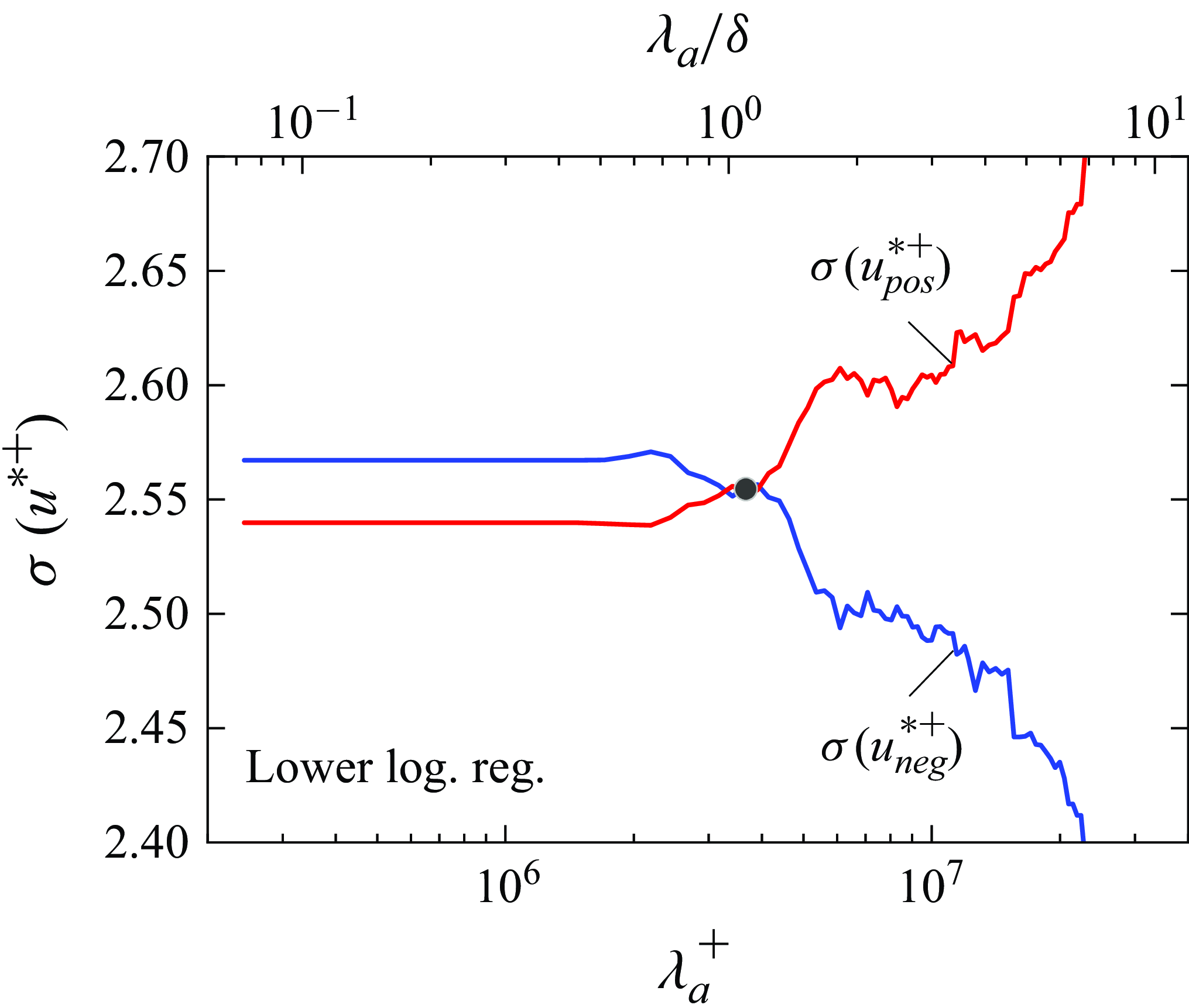
Standard deviation of conditional samples of universal signal
 $\sigma (u_{{neg}}^{*+})$
and
 $\sigma (u_{{pos}}^{*+})$
at
 $Re_{\tau } = 3.3 \times 10^{6}$
, versus the cutoff wavelength
 $\lambda _{a}^{+}$
at which footprint scales are split (
 $z$
= 0.9 m). The black dot highlights the optimal cutoff wavelength
 $\lambda _{opt}/\delta \simeq 1.2$
.

4.1. The multiscale effect
The multiscale effect has been recently revealed in ASL (Liu et al. Reference Liu, Wang and Zheng2019), which means that not all of the scales of motions have an amplitude modulation effect between them, but only specific motions do. An accurate quantification of amplitude modulation relies more on the identification of large-scale modulating motions rather than small-scale modulated motions. A multiscale amplitude modulation is further demonstrated by Liu et al. (Reference Liu, He and Zheng2023) in particle-laden ASL. Therefore, the multiscale effect is a necessity of (3.1), the amplitude modulation of
 $u^{*+}$
by
 $u_{S}^{+}$
is emphasized. Since
 $u_{S}^{+}$
comprises motions with various wavelengths of the flow, those scales which are pertinent to modulation, denoted by
 $\hat {u}_{S}^{+}$
, should be discerned. Consequently, (3.1) could be rewritten as (here, the time shift
 $\tau _{a}^{+}$
is temporarily neglected for the sole concentration on the multiscale effect)
 \begin{equation} u_{p}^{+}(z^{+},t^{+}) = u^{*+}(z^{+},t^{+}) + \Gamma (z^{+})u^{*+}(z^{+},t^{+})\hat {u}_{S}^{+}(z^{+},t^{+}) + u_{S}^{+}(z^{+},t^{+}), \end{equation}
where
 $\hat {u}_{S}^{+}=\left .u_{S}^{+}\right |_{\lambda _{x}^{+}\gt \lambda _{a}^{+}}$
, and
 $\lambda _{a}^{+}$
is the cutoff wavelength between the scales that dominate modulation and others. The detrended signal could thus be given by (variables
 $z^{+}$
and
 $t^{+}$
omitted)
 \begin{equation} u_{d}^{+} = u^{*+} + \Gamma u^{*+}\hat {u}_{S}^{+}, \end{equation}
and the universal signal is of the form
 \begin{equation} u^{*+} =\frac {u_{d}^{+}}{1 + \Gamma \hat {u}_{S}^{+}}, \end{equation}
where
 $\hat {u}_{S}^{+}$
cannot be a priori perceived and is to be investigated. A reasonable is to iteratively search for
 $\lambda _{a}$
that theoretically gives a zero degree of amplitude modulation of
 $u^{*+}$
. To assess the quality of
 $u^{*+}$
, a quantity that is susceptible to amplitude modulation is required, albeit the PDFs mentioned above could be used for examining large-scale relevance. In the theory of stochastic process, the amplitude of a signal during a period of time could be quantified by local standard deviation
 $\sigma (\bullet )$
. Provided
 $\sigma (\{u_{{neg}}^{*+}\})$
is equal to
 $\sigma (\{u_{{pos}}^{*+}\})$
(
 $\{u_{{neg}}^{*+}\}$
and
 $\{u_{{pos}}^{*+}\}$
are, respectively, conditional samples of
 $u^{*+}$
during a negative and positive footprint), the amplitude of
 $u^{*+}$
would no longer alter due to large scales, which indicates that the amplitude modulation is ideally removed. Above all, the local standard deviation could be used as a sensible indicator in the process of demodulation.
Figure 5 shows
 $\sigma (u_{{neg}}^{*+})$
and
 $\sigma (u_{{pos}}^{*+})$
(‘
 $\{ \}$
’ omitted) with
 $\lambda _{a}$
at
 $z=0.9$
m. It clearly reveals that the performance of
 $u^{*+}$
is highly dependent on the selection of
 $\lambda _{a}$
. For
 $\lambda _{a}\approx$
1.2
 $\delta$
, a unique coincidence between
 $\sigma (u_{{neg}}^{*+})$
and
 $\sigma (u_{{pos}}^{*+})$
could be noticed, which illustrates that the amplitude of
 $u^{*+}$
exhibits a perfect irrelevance to footprints, and thus a satisfactory demodulation has been conducted. Denoting the corresponding wavelength as the optimal cutoff wavelength
 $\lambda _{opt}$
, once a longer value is set to a pass-filter, the difference between
 $\sigma (u_{{neg}}^{*+})$
and
 $\sigma (u_{{pos}}^{*+})$
would distinctly increase, which implies that the footprint scales with the streamwise wavelength longer than approximately 1.2
 $\delta$
are dominant in the modulation on
 $u^{*+}$
. As soon as they are absent from
 $\hat {u}_{S}^{+}$
, the amplitude of
 $u^{*+}$
would literally still be ‘modulated’. Moreover, the smoothness of
 $\sigma (u^{*+})$
when smaller cutoffs are chosen is evident in that
 $u_{S}^{+}$
comprises only those scales with
 $\lambda _{x}^{+}\gt \lambda _{x T}^{+} \approx 2 \times 10^{6}$
, and a low-pass filter is in vain herein for
 $\lambda _{a}^{+}\lt \lambda _{x T}^{+}$
, i.e.
 $\hat {u}_{S}^{+}=u_{S}^{+}$
. This again highlights that if the multiscale effect is not properly accounted for in the model, the universal signal extracted via demodulation would still be mildly sensitive to footprints, which could explain to some extent the mismatch therein.
Probability density functions of
 $u_{{neg}}^{*+}$
and
 $u_{{pos}}^{*+}$
with different
 $\lambda _{a}$
are shown in figure 6. Since
 $\hat {u}_{S}^{+}$
corresponds to ‘large scales’ in the common sense, some nominal cutoff wavelengths are selected for demonstration (
 $\lambda _{a} / \delta \gt 1$
, LSM;
 $\lambda _{a} / \delta \gt 3$
, VLSM at moderate
 $Re$
;
 $\lambda _{a} / \delta \gt 7$
, VLSM with larger scale at extreme
 $Re$
). Specially, results of the original scheme without the multiscale effect arranged (3.1) is denoted by ‘none’. Although it is less discernible, the effects of
 $\lambda _{a}$
on the demodulation process could also be observed: compared with the original scheme, as
 $\lambda _{a}$
approaches
 $\lambda _{opt}$
, the two PDFs become relatively similar because the scales that are not much pertinent to the amplitude modulation (i.e.,
 $\lambda _{x}\lesssim 1.2 \delta$
in
 $u_{S}^{+}$
) would no longer be introduced into (4.3) or interfere in the demodulation. Otherwise, an exceedingly large
 $\lambda _{a}$
would render those which dominate the amplitude modulation are absent from the process, and that
 $u_{{neg}}^{*+}$
differs significantly from
 $u_{{pos}}^{*+}$
, which would lead to a failed demodulation. This emphasizes the significance of prudently seizing the pertinent modulation scales in footprint for model refinement.
Probability density functions of conditional samples of universal signal PDF
 $(u_{{neg}}^{*+})$
(blue lines) and PDF
 $(u_{{pos}}^{*+})$
(red lines) at
 $Re_{\tau } = 3.3 \times 10^{6}$
, versus the cutoff wavelength
 $\lambda _{a}$
at which footprint scales are split (
 $z$
= 0.9 m). Here
 $\lambda _{a}$
in each case is marked on the axis below, and ‘none’ corresponds to the scheme in which multiscale effect has been ignored.

Finally, the case of the upper logarithmic region is discussed. Since the superposition by input signals upon those locations has been revealed, the ‘imprint’
 $u_{S}^{+}$
would also modulate the local universal signals therein, and thus clues about the modulation scales
 $\hat {u}_{S}^{+}$
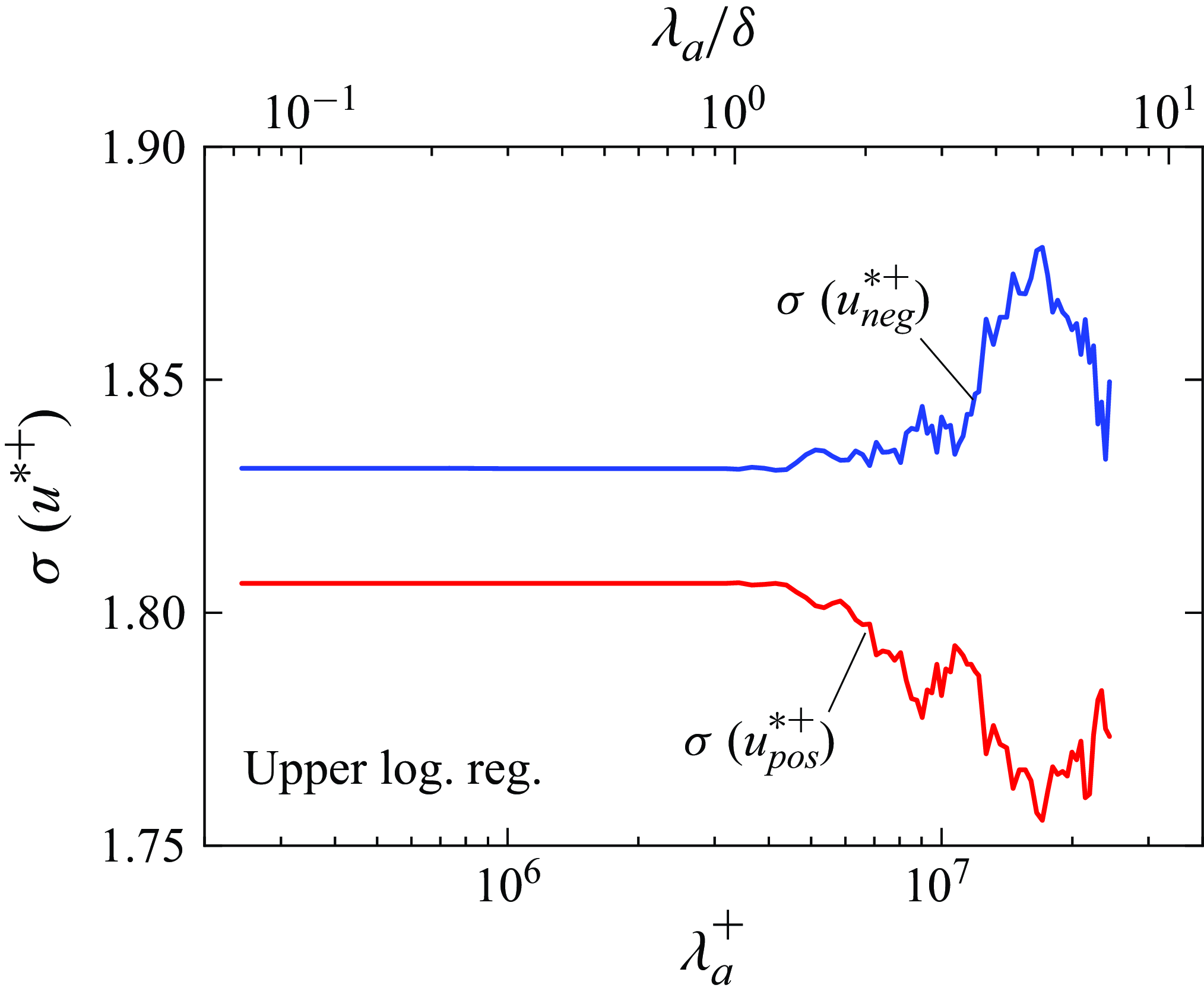
are noted. Figure 7 shows the variation in
 $\sigma (u_{{neg}}^{*+})$
and
 $\sigma (u_{{pos}}^{*+})$
with
 $\lambda _{a}$
at
 $z=30$
m. A different result from that in the lower logarithmic region could be observed herein: whatever
 $\lambda _{a}$
is selected,
 $\sigma (u_{{neg}}^{*+})$
differs far from
 $\sigma (u_{{pos}}^{*+})$
. This manifests that the amplitude of
 $u^{*+}$
would always display a correlation to ‘imprint’ and is thus large-scale-modulated. Basically, the original scheme without the multiscale effect arranged (when smaller
 $\lambda _{a}$
is chosen) is reconsidered and
 $\sigma (u_{{neg}}^{*+})$
and
 $\sigma (u_{{pos}}^{*+})$
would not be actually consistent. Hence, it could be deduced that in the upper logarithmic region, none of the cutoffs could cater perfectly to the demodulation, and that (4.1) could not be satisfied in at least the process of extracting the universal signal. As what will be introduced subsequently, this might be due to another particular in amplitude modulation, the time shift, which has not yet been discussed. Nevertheless, there is no doubt that the multiscale effect should be appropriately accounted for in the amplitude modulation part of the predictive models. The surrogate
 $\hat {u}_{S}^{+}$
of
 $u_{S}^{+}$
in the nonlinear term could exclude those scales that are less pertinent to the amplitude modulation and as much large-scale information in the universal signal could be consequently eliminated as possible.
Standard deviation of conditional samples of universal signal
 $\sigma (u_{{neg}}^{*+})$
and
 $\sigma (u_{{pos}}^{*+})$
(at
 $Re_{\tau } = 3.3 \times 10^{6}$
), versus the cutoff wavelength
 $\lambda _{a}^{+}$
at which footprint scales are split (
 $z$
= 30 m).

4.2. Relative time shift in amplitude modulation
The time shift in amplitude modulation represents the relative shift between the superposition imprint and the modulated small scales. Since the nonlinear modulation term in the models is in the form of a product of time series, even though the time shift is seemingly trivial in some cases, gigantic mismatch between the prediction and actuality would accumulate in long-term investigations, which is by no means acceptable in the time domain.
In a boundary layer of a wind tunnel at
 $Re_{\tau }=14750$
, Baars et al. (Reference Baars, Talluru, Hutchins and Marusic2015) separated the large-scale and small-scale components of the streamwise fluctuations by applying a nominal cutoff wavelength
 $\lambda _{x}^{+}=7000$
and computed the amplitude modulation coefficient
 $R_{AM}$
at
 $z^{+}=4.33$
to
 $z / \delta =1.45$
. In an isocorrelation map they noted the time shift in capturing
 $R_{AM}$
. Similarly, the counterpart calculated in ASL is shown in figure 8, with the procedures specified as follows. Firstly, the measured signals at each height are filtered to separate the nominal large and small components
 $u_{l}(t)$
,
 $u_{s}(t)$
(it should be noted that although the multiscale effect is proved,
 $\lambda _{x}=\delta$
is primitively selected as the cutoff wavelength herein to align with Baars et al. (Reference Baars, Talluru, Hutchins and Marusic2015)). Further, the Hilbert transform is used to obtain the envelope of the small-scale series
 $E [u_s(t) ]$
and a low-pass filter is then applied to sift
 $E_l[u_s(t)]$
with a passband of
 $\lambda _{x}\gt \delta$
(see Mathis et al. Reference Mathis, Hutchins and Marusic2009). Finally, the time shift in amplitude modulation
 $\tau _{AM}$
would be a priori assumed to adjust the large-scale series
 $u_l(t)$
and the amplitude modulation coefficient could be calculated as
 \begin{equation} R_{AM} = \frac {\overline {E_{l}[u_{s}(t)]u_{l}(t-\tau _{AM})}}{\sqrt {\overline {E_{l}^{2}[u_{s}(t)]}}\sqrt {\overline {u_{l}^{2}(t-\tau _{AM})}}}, \end{equation}
by which the theoretical
 $\tau _{AM}$
that gives a maximal correlation between
 $u_l(t-\tau _{A M})$
and
 $E_l[u_s(t)]$
(the peak
 $R_{AM}$
) could be revealed.
Isocorrelation map of the amplitude modulation coefficient
 $R_{AM}$
at
 $Re_{\tau } = 3.3 \times 10^{6}$
; level range
 $-$
0.3–0.3 in steps of 0.05. The mean velocity at
 $z$
= 30 m is used as the free stream velocity
 $U_{\infty }$
in the outer-scaled time shift. Here ‘
 $-$
Ve Corr.’ or ‘
 $+$
Ve Corr.’ stand for where
 $R_{AM}$
is negative or positive; the symbol
 $\bigcirc$
marks peaks of
 $R_{AM}$
and light grey border of it means a notably small absolute value in here in comparison with the opposite peak.

Initially, we focus on the case of
 $\tau _{AM}=0$
shown by the horizontal dashed line in the figure, which corresponds to the results in early studies where the time shift was not specifically discussed (Schlatter et al. Reference Schlatter, Örlü, Li, Brethouwer, Fransson, Johansson, Alfredsson and Henningson2009; Mathis et al. Reference Mathis, Hutchins and Marusic2011). At first glance,
 $R_{AM}$
is positive in the near-wall region and decreases progressively to zero for higher
 $z$
, above which a reversal in correlation could be perceived. This is aligned with the results reported in previous studies that when positive large scales occur, the amplitude of the small-scale fluctuations in the near-wall region would be increased, whereas that in the outer region would be suppressed on the contrary. In reality, this might be an artefact due to the calculation mode. Equation (4.4) is in the form a time-domain correlation coefficient, and if the relative shift between signals is ignored, chances are that the coefficient would be underestimated in that the degree of correlation has been blurred. As
 $\tau _{AM}$
is accounted for, the map of
 $R_{AM}$
in ASL and the wind tunnel boundary layer are qualitatively comparable despite the span of two orders of magnitude in
 $Re_{\tau }$
. In the range
 $10^{-2}\lt z / \delta \lt 10^{-1}$
,
 $\tau _{AM}$
is assumed to be positive or negative, respectively, and a negative or positive peak of
 $R_{AM}$
would accordingly appear. The intensity of those peaks is significantly higher than that when
 $\tau _{AM}=0$
. This assures the necessity of searching for the relative time shift to clearly reveal the correlation between
 $E_l(u_s)$
and
 $u_{l}$
and thus accurately capture the degree of amplitude modulation.
The time shifts corresponding to the occurrences of positive and negative
 $R_{AM}$
peaks are here defined as the peak time shift
 $\tau _{AM1}$
and
 $\tau _{AM2}$
, respectively (hollow symbols in figure 8). The revelation of multipeak coefficient is theoretically anticipated as shown in figure 9(b) which exhibits the actuality of
 $u_{l}(t)$
and
 $E_l[u_s(t)]$
in the time domain, between which a relative time shift should exist. Provided
 $\tau _{AM}$
in (4.4) is assumed negative,
 $u_{l}(t)$
would be seen as if shifted forward in the time axis. Owing to the quasiperiodic nature of turbulence (Dennis Reference Dennis2015; Marusic et al. Reference Marusic, McKeon, Monkewitz, Nagib, Smits and Sreenivasan2010b
), one could anticipate capturing a positive peak correlation between
 $u_{l}$
and
 $E_l[u_s]$
after applying a shift
 $\left |\tau _{A M 1}\right |$
on
 $u_{l}$
within a quasiperiod of it, as shown in figure 9(a) where
 $R_{AM}$
appears to reach a positive peak. In contrast, a positive presumed
 $\tau _{AM}$
means that
 $u_{l}$
would be adjusted backwards. After applying the shift
 $\left |\tau _{A M 2}\right |$
,
 $u_{l}$
would appear as a negative peak correlation to
 $E_l[u_s]$
at exactly half a quasiperiod away from it as in figure 9(c), which consequently leads to a negative peak of
 $R_{AM}$
. An excessively large time shift preset may cause
 $u_{l}$
to be aligned with
 $E_l[u_s]$
in other quasiperiods, say in the near-wall region for
 $\left |\tau _{A M}^{+}\right |\gtrsim 1.5 \times 10^5$
in figure 8. That
 $R_{AM}$
altered in sign indicates a collapse of
 $u_{l}$
with
 $E_l[u_s]$
in adjacent quasiperiods, which further clarifies the multipeak nature of
 $R_{AM}$
. Those peaks of the amplitude modulation coefficient might shed light on the perspective that at least in the process of demodulation, it should be the degree of the correlation between the large scales and the envelope of small scales (i.e. how much the small scales are modulated) that matters more in accordingly removing such an effect rather than whether the amplitude of small-scale signals are enhanced or suppressed, which is explicitly reflected in the magnitude of the amplitude modulation coefficient.
Multipeak amplitude modulation coefficient on account of the time shift
 $\tau _{AM}$
; signals are simplified into sinusoidal curves for clarity. The black line shows the low-pass filtered envelope of the small-scale signal
 $E_l[u_s(t)]$
; the red line shows the large-scale signal
 $u_{l}(t)$
. Panel (b) exhibits the actuality; the dashed lines in (a) and (c) exhibit
 $u_{l}(t-\tau _{A M 1})$
and
 $u_{l}(t-\tau _{A M 2})$
when
 $u_{l}(t)$
is artificially shifted.

With regard to the time shift in amplitude modulation,
 $\tau _{a}^{+}$
in (3.1) denotes the time shift that is supposed to be accounted for in the nonlinear modulation term. Hence, the detrended signal could be given as (
 $z^{+}$
omitted)
 \begin{equation} u_{d}^{+}(t^{+}) = u^{*+}(t^{+}) + \Gamma u^{*+}(t^{+})u_{S}^{+}(t^{+}-\tau _{a}^{+}), \end{equation}
and the universal signal
 \begin{equation} u^{*+}(t^{+}) =\frac {u_{d}^{+}(t^{+})}{1 + \Gamma u_{S}^{+}(t^{+}-\tau _{a}^{+})}. \end{equation}
Since
 $\tau _{a}^{+}$
is not available and is to be investigated, one could resort to iteratively search for it with the aim of extracting
 $u^{*+}$
that would theoretically meet expectations (i.e.
 $u^{*+}$
is not modulated any longer). The corresponding captured value is defined as the optimal time shift
 $\tau _{opt}^{+}$
which reflects the actual temporal asynchrony between
 $u_{S}^{+}$
and the amplitude of
 $u^{*+}$
. Similarly, the quality of
 $u^{*+}$
is examined via keeping a track of
 $\sigma (u_{{neg}}^{*+})$
and
 $\sigma (u_{{pos}}^{*+})$
, which is shown in figure 10. It could be noted that at each height discussed herein, there would always exist one positive and one negative
 $\tau _{opt}^{+}$
that render
 $u^{*+}$
literally free from large-scale modulation. This is essentially compatible with multipeak
 $R_{AM}$
: the negative optimum means that
 $u_S^{+}(t^{+})$
would be shifted forward to maximize the positive correlation with the change in the amplitude of
 $u^{*+}$
, while the positive value means that
 $u_S^{+}(t^{+})$
would be by contrast be shifted backwards to negatively correlate with the change in the amplitude of
 $u^{*+}$
. After all, now that the actual asynchrony between the large-scale fluctuations and the change in the amplitude of small scales remains unclear, it could be possible on the other hand that a negative
 $\tau _{opt}^{+}$
leads to a negative correlation, and vice versa. In particular, it should be emphasized that both the positive and negative values of
 $\tau _{opt}^{+}$
would basically suffice in the demodulation as long as the time shift attached in the model is able to adjust
 $u_{S}^{+}$
to exhibit exactly a peak correlation with the change in the amplitude of
 $u^{*+}$
(regardless of a positive or negative one), via which the amplitude modulation effect in (3.1) could be decently accounted for, thankfully, without determining which
 $\tau _{opt}^{+}$
to pick.
Standard deviation of conditional samples of universal signal
 $\sigma (u_{{neg}}^{*+})$
and
 $\sigma (u_{{pos}}^{*+})$
at
 $Re_{\tau } = 3.3 \times 10^{6}$
, versus the time shift
 $\tau _{a}^{+}$
attached to the model. Results are from the lower (
 $z$
= 0.9 m), central (
 $z$
= 7.15 m) and upper (
 $z$
= 30 m) logarithmic region. The black dot highlights the optimal time shift
 $\tau _{opt}^{+}$
.

Figure 11 shows the PDFs of
 $u_{{neg}}^{*+}$
and
 $u_{{pos}}^{*+}$
with
 $\tau _{a}^{+}$
at
 $z=0.9$
and 30 m. It is obvious that
 $\tau _{a}^{+}$
would affect the degree of large-scale dependence of
 $u^{*+}$
, say the function of
 $u_{{neg}}^{*+}$
is most comparable with that of
 $u_{{pos}}^{*+}$
when it is in proximity to
 $\tau _{opt}^{+}$
, which represents that most of the amplitude modulation effect would have been removed. Once the value is set far from the optimum
 $\tau _{opt}^{+}$
, those conditional samples would reflect considerably differently in statistics owing to an inadequate demodulation. The variations in PDF(
 $u^{*+}$
) with
 $\tau _{a}^{+}$
are seen to be consistent with what is observed in
 $\sigma (u^{*+})$
in figure 10. This evidently proves once again the necessity to arrange the time shift in predictive models for refinement and that the accuracy of it should be prudently noted.
Probability density functions of conditional samples of universal signal PDF
 $(u_{{neg}}^{*+})$
(blue lines) and PDF
 $(u_{{pos}}^{*+})$
(red lines) at
 $Re_{\tau } = 3.3 \times 10^{6}$
, versus the time shift
 $\tau _{a}^{+}$
attached to the model. Results are from the lower (
 $z$
= 0.9 m) and upper (
 $z$
= 30 m) logarithmic region.
 $\tau _{a}^{+}$
in each case is marked on the axis in the middle on upward and downward scales.

Another question is whether the optimal time shift
 $\tau _{opt}^{+}$
agrees with the peak time shifts
 $\tau _{A M 1}^{+}$
and
 $\tau _{A M 2}^{+}$
, which is detailed in figure 12. For convergence and robustness,
 $\tau _{opt}^{+}$
has been searched in the datasets with
 $Re_\tau =(2.0-4.5) \times 10^6$
(i.e. datasets 1–12 are involved and exhibited). Since
 $\tau _{opt}^{+}$
is not unique and the purpose to decently shape the amplitude modulation could be achieved with either a positive or a negative optimum, we pick those
 $\tau _{opt}^{+}$
that are in close proximity to zero, in line with the recognition that modulation time shifts are negative in the near-wall region but positive farther away as suggested by previous studies (Baars et al. Reference Baars, Talluru, Hutchins and Marusic2015; Hutchins et al. Reference Hutchins, Monty, Ganapathisubramani, H.C.H. and Marusic2011). The comparison of those time shifts obtained in the two methods shows, however, that they are not strictly consistent. Common sense is that a deterministic physical law would not be supposed to depend on how it has been analysed. This might imply that a solitary introduction of modulation time shift to the model is also seemingly insufficient.
Optimal time shift
 $\tau _{opt}^{+}$
(black dots) obtained in the process of demodulation and peak time shift
 $\tau _{AM1}^{+}$
,
 $\tau _{AM2}^{+}$
(red and blue triangles) obtained in process of computing amplitude modulation coefficient. Location of the required input to the model is labelled.

The discrepancy between
 $\tau _{opt}^{+}$
and
 $\tau _{A M 1}^{+}$
(as well as
 $\tau _{A M 2}^{+}$
) is herein discussed. Since they are derived from two pairs of signals with different modes of scales (
 $u_{S}$
and
 $u^{*}$
;
 $u_{l}$
and
 $u_{s}$
), it is not surprising to notice disagreements. In order to demonstrate further, the procedures of revealing the peak time shifts are recalled in the cases of applying the cutoff wavelength
 $\lambda _{xcr}=0.25 \delta, 0.5\delta, \delta, 2\delta, 3\delta$
to separate the signals that are measured in the lower (
 $z=0.9$
m) and upper (
 $z=30$
m) logarithmic region. Regarding those with
 $\lambda _x\gt \lambda _{x c r}$
and
 $\lambda _x\lt \lambda _{x c r}$
as the modulating large scales
 $u_{l}$
and the modulated small scales
 $u_{s}$
, respectively,
 $R_{AM}$
in (4.4) is calculated with varying presumed
 $\tau _{AM}$
as shown in figure 13. The results indicate that the peaks of
 $R_{AM}$
(shown by star symbols) captured within signal pairs of several cutoffs would appear at different
 $\tau _{AM}$
. In other words, the usage of signals with different scales will inversely derive the peak time shifts with a large discrepancy. In the upper logarithmic region, the discrepancy between those peak time shifts corresponding to different cutoff wavelengths would be even obvious for the flow scale cascade in the upper logarithmic zone being more complicated, and as shown in figure 13(b), which leads to a large discrepancy between
 $\tau _{opt}^{+}$
and
 $\tau _{A M 1}^{+} / \tau _{A M 2}^{+}$
at this point.
Finally, it should be mentioned that the peaks of
 $R_{AM}$
would always be exposed at particular
 $\tau _{AM}$
albeit different cutoff wavelengths have been selected. However, these peaks vary in magnitude and, most notably, not each peak deserves attention. On the one hand, the multiscale nature of amplitude modulation demonstrates that
 $R_{AM}$
would be significantly underestimated if those scales innocent of the process are ambiguously enclosed in the signals. For most of the peaks, inevitably, they are not able to reflect the actual degree of the amplitude modulation due to the blurred coefficient. As it was discussed, searching for the time shift therein relies chiefly on the discovery of
 $R_{AM}$
peaks, which definitely requires clues of the multiscale. Specifically, the scales that are not so pertinent to the amplitude modulation would display distinctively compared with those responsive therein, which consequently could interfere with the process of revealing the peak
 $R_{AM}$
and thus
 $\tau _{AM}$
. On the other hand, however, discerning the main characters in the amplitude modulation also calls for an investigation on
 $R_{AM}$
among scales in advance, for which the time shift must not be treated arbitrarily to find the peaks or else wrong judgments would be made, for example at
 $\tau _{A M}^{+}=0$
in figure 13 (as if the modulation time shift is neglected). To conclude, those two factors (namely the multiscale performance and the time shift in the amplitude modulation) have been coupled and each of them could not be surveyed in the absence of the other. This indicates that they are supposed to be simultaneously taken into account with the aim of capturing the actual magnitude of amplitude modulation and thus conducting a satisfactory demodulation.
Amplitude modulation coefficient
 $R_{AM}$
in signal pairs (at
 $Re_{\tau } = 3.3 \times 10^{6}$
) with different cutoff wavelengths
 $\lambda _{xcr}=0.25 \delta$
, 0.5
 $\delta$
,
 $\delta$
, 2
 $\delta$
, 3
 $\delta$
at varying time shift
 $\tau _{AM}^{+}$
; the symbol
 $\bigstar$
marks when
 $R_{AM}$
peaks appear. Here (a)
 $z$
= 0.9 m; (b)
 $z$
= 30 m, and negative
 $R_{AM}$
peaks are zoomed to clearly reveal the difference in
 $\tau _{AM}^{+}$
. Note the difference in the abscissa from that in (a).

5. Improved model under dual-factor coupling
The analyses in previous sections demonstrate the necessity of accounting for the multiscale effect and the time shift to precisely quantify the degree of the amplitude modulation as well as the refinement of the universal signal owing to the attachment of those two factors, respectively, to the model. However, if they are individually investigated, chances are the maximal peaks of the amplitude modulation coefficient would not be distinctly exposed as what was discussed above, which conversely blocks the way to reach the true modulation-related scales and the time shift. Therefore, the only sensible method would be to simultaneously take them into consideration for improved predictions.
5.1. Amplitude modulation taking account of multiscale effect and time shift
In this section, both the multiscale effect and the time shift in the amplitude modulation have been accounted for and a refined scheme in light of them is presented to reveal the factual degree of the amplitude modulation.
The amplitude modulation coefficient
 $R_{AM}$
would be calculated as modified below. With regard to the multiscale effect therein, the cutoff wavelengths
 $\lambda _{L}$
and
 $\lambda _{S}$
are iteratively altered and applied into the measured signal for separating
 $\hat {u}_{l}(t)$
(large-scale components with
 $\lambda _{x}\gt \lambda _{L}$
) and
 $\hat {u}_{s}(t)$
(small-scale components with
 $\lambda _{x}\lt \lambda _{S}$
) respectively, by which the modulation among hierarchical flow scales could be minutely weighed. As long as those that are responsive to the amplitude modulation have been called, a prominently strong
 $R_{AM}$
would be captured. In another aspect, the modulation time shift
 $\tau _{AM}$
is a priori presumed as introduced in § 4.2 to iteratively adjust
 $\hat {u}_{l}(t)$
so that the correlation peaks with the small-scale envelope
 $E_{l}[\hat {u}_{s}(t)]$
could appear. Thus,
 $R_{AM}$
is expressed as
 \begin{equation} R_{AM} = \frac {\overline {E_{l}[\hat {u}_{s}(t)]\hat {u}_{l}(t-\tau _{AM})}}{\sqrt {\overline {E_{l}^{2}[\hat {u}_{s}(t)]}}\sqrt {\overline {\hat {u}_{l}^{2}(t-\tau _{AM})}}}, \end{equation}
and it is sensitive to
 $\lambda _{L}$
,
 $\lambda _{S}$
and
 $\tau _{AM}$
.
Figure 14 shows the isocorrelation map of
 $R_{AM}$
with three variables at
 $z=0.9$
m and
 $z=30$
m. Undoubtedly,
 $R_{AM}$
exhibits both multiscale and multipeak quality. In one aspect, very active feedback of
 $R_{AM}$
could only be observed in the vicinity of specific
 $\lambda _{L}$
and
 $\lambda _{S}$
due to the multiscale nature of the process. In the other, the magnitude of
 $R_{AM}$
would vary with
 $\tau _{AM}$
, which represents the shuttle between positive and negative correlations of
 $\hat {u}_{l}$
and
 $E_{l}(\hat {u}_{s})$
. It should be noted that compared with what exists in the near-wall region, the coherent structures in the upper would self-organize in larger length scales as well as extended time scales, and those that are dominating in the amplitude modulation would also feature longer wavelengths. This leads consequently to the extremes of
 $R_{AM}$
occurring at relatively larger
 $\lambda _{L}$
. The alternation in the sign of the correlation would also feature an elongated
 $\tau _{AM}$
span. For capturing the factual degree of the amplitude modulation, the global peaks of
 $R_{AM}$
emerge and are defined as the modified amplitude modulation coefficient
 $R_{AM-mod}$
in that each of the essentials of the process has been properly caredfor. Further, the corresponding cutoffs and interval are defined as the modified cutoff wavelength of modulating scales
 $\lambda _{L-mod}$
, the modified cutoff wavelength of modulated scales
 $\lambda _{S-mod}$
and the modified peak time shift
 $\tau _{AM-mod}$
.
Isocorrelation map of the amplitude modulation coefficient
 $R_{AM}$
at
 $Re_{\tau } = 3.3 \times 10^{6}$
, along with cutoff wavelength
 $\lambda _{L}^{+}$
(for isolating large-scale modulating signal),
 $\lambda _{S}^{+}$
(for isolating small-scale carrier signal) and modulation time shift
 $\tau _{AM}^{+}$
; level range is tagged beside. Here (a)
 $z$
= 0.9 m; (b)
 $z$
= 30 m.

Wall-normal evolution of amplitude modulation coefficient. The red dots show positive peaks of the modified amplitude modulation coefficient
 $R_{AM-mod}$
at
 $Re_{\tau } = (2.0-4.5) \times 10^{6}$
; the black solid line show the peak amplitude modulation coefficient suggested by Liu et al. (Reference Liu, Wang and Zheng2019) in the absence of time shift (
 $Re_{\tau }=(2.8-3.3)\times 10^{6}$
); the orange line and black dashed lines show the results that are given by Mathis et al. (Reference Mathis, Hutchins and Marusic2009) with a cutoff wavelength
 $\lambda _{xcr}= \delta$
in the ASL and wind tunnel, respectively (here denoted by
 $R_{AM-M}$
).

For convenience, the positive
 $R_{AM-mod}$
peaks are attained for comparison with the results from previous studies in figure 15. In the lower logarithmic region (
 $z/\delta \lesssim 0.05$
),
 $R_{AM-mod}$
is seen to be stronger than that in all previous results thanks to the refinement of the correlation, so that the similarity between the modulator and the modulated small-scale amplitude is clearly presented. The results suggested by Liu et al. (Reference Liu, Wang and Zheng2019) fail to reflect the modulation time shifts and the correlations would theoretically be doomed to be underestimated in comparison with
 $R_{AM-mod}$
with an overall difference of
 $\sim$
20 %. The
 $R_{AM-M}$
given by Mathis et al. (Reference Mathis, Hutchins and Marusic2009) have neither eliminated the interference by other scales innocent of the modulation nor explicitly put up any time asynchrony in the process and eventually exhibits in a much lower level. Generally, however, the widespread acknowledgment is confirmed that the amplitude modulation coefficient would gradually decrease logarithmic–linearly in level as
 $z/\delta$
climbs below the nominal centre of the logarithmic region, regardless of whether it has been calculated in a more decent way or not.
In the region farther away from the wall (
 $z/\delta \gtrsim 0.05$
), we have observed a notable phenomenon that may have never been reported before:
 $R_{AM-mod}$
would significantly reboost with
 $z/\delta$
to a correlation of
 $\sim$
0.5 at the highest detectable position in the scope of this study, which implies that a remarkable level of amplitude modulation would also occur in the upper logarithmic region among specific motions. The strength of this effect herein may even be greater than that in the near-wall region where interactions of flow scales are reckoned the most conspicuous in common sense. To specify, it should be recalled that in essence,
 $R_{AM}$
is in a form of correlation whose intensity would always shape the similarity between the large scales and the amplitude of small scales regardless of whether the value is positive or negative. Therefore, that
 $R_{AM-M}$
decrease to negative values as
 $z/\delta$
climbs out of the central logarithmic region and further amplify in magnitude despite the minus sign could indicate, in fact, the reboosting amplitude modulation in here as presented in this study. As what is discussed above, Mathis et al. (Reference Mathis, Hutchins and Marusic2009) fails to take the modulation time shift into account and thus a negative correlation of the signal pairs happens to be captured. In this study, the positive and negative values of
 $R_{AM-mod}$
are stringently discriminated, which visually leads to the contradiction of the amplitude modulation coefficient.
So far, the amplitude modulation in ASL on account of the multiscale effect and the modulation time shift has been investigated in detail. The modified amplitude modulation coefficient
 $R_{AM-mod}$
, which is susceptible to additional cutoffs and time shift compared with that in previous works, is evidently stronger and would provide more accurate feedback of the effect at each height. Furthermore, one could also pin the hopes on digging up the amplitude modulation happening in much farther away from the wall, which is seen to be even comparable to the near-wall region.
5.2. Demodulation taking account of multiscale effect and time shift
In § 4, the refinements of the predictive model owing to the account on the multiscale effect and the modulation time shift have been individually demonstrated. Consequently, those two particulars are dually put on in this part in pursuit of a further optimization of the model. Above all, note that the predictive signal
 $u^{+}$
should be given by
 \begin{equation} u^{+}(z^{+},t^{+}) = u^{*+}(z^{+},t^{+}) + \Gamma (z^{+})u^{*+}(z^{+},t^{+})\hat {u}_{S}^{+}(z^{+},t^{+}-\tau _{a}^{+}) + u_{S}^{+}(z^{+},t^{+}), \end{equation}
in which the footprint is enrolled via the SLSE following Baars et al. (Reference Baars, Hutchins and Marusic2016). The multiscale effect and the modulation time shift are inclusively embedded in the nonlinear term of the model, which leads to a change in the form of it. Here
 $\hat {u}_{S}^{+}$
derives from
 $u_{S}^{+}$
and corresponds to the component that would significantly exert amplitude modulation on
 $u^{*+}$
. Here
 $\tau _{a}^{+}$
reflects the time shift in the modulation.
The detrended signal could thus be given by (
 $z^{+}$
omitted)
 \begin{equation} u_{d}^{+}(t^{+}) = u^{*+}(t^{+}) + \Gamma u^{*+}(t^{+})\hat {u}_{S}^{+}(t^{+}-\tau _{a}^{+}), \end{equation}
with the universal signal as
 \begin{equation} u^{*+}(t^{+}) =\frac {u_{d}^{+}(t^{+})}{1 + \Gamma \hat {u}_{S}^{+}(t^{+}-\tau _{a}^{+})}, \end{equation}
where
 $\hat {u}_{S}^{+}(t^{+}-\tau _{a}^{+})=u_{S}^{+}(t^{+}-\tau _{a}^{+})|_{\lambda _{x}^{+}\gt \lambda _{a}^{+}}$
. Here
 $\lambda _{a}^{+}$
denotes the cutoff wavelength between the scales that are pertinent to the amplitude modulation and others. Here
 $\tau _{a}^{+}$
denotes the time shift in this process. Those two quantities ought to be investigated in advance for subsequent demodulation, which has been individually conducted in previous sections and highlights their respective optimums,
 $\lambda _{opt}$
and
 $\tau _{opt}$
. However, as what was discussed, a neglect of each quantity could lead to unreliable conclusions. Accordingly, global searches for optimums of
 $\lambda _{a}$
and
 $\tau _{a}$
are simultaneously performed with a criterion that the amplitude of
 $u^{*+}$
would not any longer be modulated, which could be mirrored in the local standard deviation.
Figure 16 exhibits the difference of the local standard deviations
 $\Delta \sigma =|\sigma (u_{{neg}}^{*+})-\sigma (u_{{pos}}^{*+})|$
with
 $\lambda _{a}$
and
 $\tau _{a}$
at
 $z=0.9$
m and
 $z=30$
m. Intuitively, a smaller
 $\Delta \sigma$
indicates more indiscernible differences between the localized amplitude of
 $u_{{neg}}^{*+}$
and
 $u_{{pos}}^{*+}$
, and
 $u^{*+}$
would thus to a large extent meet the anticipation of a thorough demodulation. As what could be observed in figure 16, at each height, provided
 $\lambda _{a}$
is presumed a moderate value,
 $\Delta \sigma$
would always temporarily shrink to the minimum at a positive and a negative
 $\tau _{a}$
over a wide band of wavelength. Note again that
 $u_{S}^{+}$
comprises only the large scales with
 $\lambda _{x}\gt \lambda _{xT}$
, therefore the filtering would be in vain when
 $\lambda _{a}\lt \lambda _{xT}$
, in another words,
 $\hat {u}_{S}^{+}=u_{S}^{+}$
. That
 $\Delta \sigma$
could dwindle to relatively small values at specific
 $\tau _{a}$
when a short
 $\lambda _{a}$
is chosen would imply that even if the multiscale effect is ignored, the demodulation is seen, at least to some degree, effective as expected. However,
 $\Delta \sigma$
has not yet reached the lowest level, which does not correspond to the required global optimums. As
 $\lambda _{a}$
increases, those
 $\tau _{a}$
that cultivate the minimum of
 $\Delta \sigma$
would also alter, which could be attributed to the change of the time scales of
 $\hat {u}_{S}^{+}$
. The global minimum
 $\Delta \sigma _{\textrm {{min}}}$
could be phenomenally captured at a special
 $\lambda _{a}$
threshold, above which the differences between the
 $u^{*+}$
samples become evidently larger. In fact, the scales that dominate the amplitude modulation have been sifted out of
 $\hat {u}_{S}^{+}$
with longer
 $\lambda _{a}$
, which hinders the demodulation.
In summary, the corresponding global optimums
 $\lambda _{opt-mod}$
and
 $\tau _{opt-mod}$
when
 $\Delta \sigma _{ {{min}}}$
emerge are the candidates that offer the most desirable
 $u^{*+}$
after demodulation, which are referred to as the modified optimal cutoff wavelength and the modified optimal time shift, respectively.
Isocontour map of the absolute difference in local standard deviations of universal signal
 $\Delta \sigma$
at
 $Re_{\tau } = 3.3 \times 10^{6}$
, along with the modulation time shift
 $\tau _{a}$
and the cutoff wavelength
 $\lambda _{a}$
with which
 $\hat {u}_{S}^{+}$
are isolated; level range 0.001
 $-$
0.5 in logarithmic steps. Here (a)
 $z$
= 0.9 m; (b)
 $z$
= 30 m.

Comparison between the modified optimal cutoff wavelength
 $\lambda _{opt-mod}$
, the modified optimal time shift
 $\tau _{opt-mod}$
(corresponding to the minimal difference in local standard deviations of the universal signal
 $\Delta \sigma _{{{min}}}$
) and the modified cutoff wavelength of modulating scales
 $\lambda _{L-mod}$
, modified peak time shift
 $\tau _{AM-mod}$
(corresponding to the modified amplitude modulation coefficient
 $R_{AM-mod}$
) at
 $Re_{\tau } = 3.3 \times 10^{6}$
. Error bars account for the possible accumulative errors deriving from massive calculative operations invited to time series. Here (a)
 $\lambda _{opt-mod}$
and the corresponding fitting line; (b) negative
 $\tau _{opt-mod}$
and the corresponding fitting line (
 $A$
and
 $B$
being coefficients in fitting).

Recall the modified cutoff wavelength of modulating scales
 $\lambda _{L-mod}$
and the modified peak time shift
 $\tau _{AM-mod}$
that have been defined in the process of revealing the modified amplitude modulation coefficient
 $R_{AM-mod}$
, and they are also the global optimums when the multiscale effect and the time shift are simultaneously accounted for, with which the kernel of detecting
 $\lambda _{opt-mod}$
and
 $\tau _{opt-mod}$
giving
 $\Delta \sigma _{{{min}}}$
would physically align. To specify, the aim of both methods is to radically expose the factual degree of the amplitude modulation among scales at each height. Comparisons of these quantities that are derived from two systems are exhibited in figure 17. Since the process of demodulation would invite massive calculative operations to the time series, chances are that mild accumulative errors might be brought into the results, on which the error bars in the figure are based. In addition, only the negative values
 $\tau _{opt-mod}$
and
 $\tau _{AM-mod}$
that correspond to the occurrences of
 $\Delta \sigma _{\textrm {{min}}}$
and
 $R_{AM-mod}$
are shown for reasons that have been previously detailed. The good news is that
 $\lambda _{L-mod}$
and
 $\lambda _{opt-mod}$
, as well as
 $\tau _{AM-mod}$
and
 $\tau _{opt-mod}$
, have been seen to collapse well with each other quantitatively, upon which a deduction could be made that the perception of those modulation-related scales and time shifts would not be distorted regardless of being investigated in whether the calculation of the amplitude modulation coefficients or the process of the demodulation based on the predictive model. This would throw light on the predictive model in that intensive calibrations on the parameters
 $\lambda _{a}$
and
 $\tau _{a}$
that are attached to the nonlinear term could be shrewdly bypassed with those intuitive
 $\lambda _{L-mod}$
and
 $\tau _{AM-mod}$
being surrogates. Fortunately, one could also anticipate skipping the complicated investigations on the new parameters in the prediction of other complex turbulent flows. To sum up, the coupling of the multiscale effect and modulation time shift in the refined model would mostly reflect in the term
 $\hat {u}_{S}(t-\tau _{a})$
(
 $z$
omitted), and the step-by-step procedure of obtaining it are recalled as follows. (i) Investigations on
 $\lambda _{a}$
and
 $\tau _{a}$
in calibration. The optimums of
 $\lambda _{a}$
(denoted by
 $\lambda _{opt-mod}$
) and
 $\tau _{a}$
(denoted by
 $\tau _{opt-mod}$
) could be seen in good collapse with empirical formulations of
 $\lambda _{L-mod}$
and
 $\tau _{AM-mod}$
(cutoff wavelengths and time shifts corresponding to the occurrences of amplitude modulation coefficient peaks respectively) in figure 17. (ii) A low-pass filter with a passband
 $\lambda _{x} \gt \lambda _{a}$
is applied on the predicted footprint
 $u_{S}(t)$
(Baars et al. Reference Baars, Hutchins and Marusic2016) to sift
 $\hat {u}_{S}(t)$
(an empirical formulation of
 $\lambda _{L-mod}$
could be used in determining
 $\lambda _{a}$
). (iii) The
 $\hat {u}_{S}(t)$
should be moving along the time axis according to
 $\tau _{a}$
(an empirical formulation of
 $\tau _{AM-mod}$
could be used in determining
 $\tau _{a}$
) to get
 $\hat {u}_{S}(t-\tau _{a})$
.
Wall-normal evolution of demodulation coefficients and amplitude modulation coefficients at
 $Re_{\tau } = 3.3 \times 10^{6}$
. Here (a)
 $\Gamma _{B}$
via Baars et al. (Reference Baars, Hutchins and Marusic2016) (black squares) and
 $\Gamma _{mod}$
modified in this study (red squares) obtained in the ASL, together with those given by Baars et al. (Reference Baars, Hutchins and Marusic2016) at moderate
 $Re_{\tau }$
in wind tunnel (hollow circles). (b) Relation among coefficients at
 $Re_{\tau }\simeq 7350$
: (a) raw data from Mathis et al. Reference Mathis, Hutchins and Marusic2009; Baars et al. Reference Baars, Hutchins and Marusic2016; (b)
 $Re_{\tau }\simeq 3.3\times 10^{6}$
, this study. Balls are amplitude modulation coefficients, with red lines being fittings of them. Hollow squares are raw demodulation coefficients, and solid squares are linearly amplified results of them (coefficients in the adjustments tagged beside). Here
 $z_{O}^{+}$
is the location of the input.

Another important parameter of the model is the demodulation coefficient
 $\Gamma$
. In the calibration, it visualizes the effort in demodulating and extracting the universal signal
 $u^{*+}$
, whereas in the prediction, it describes the extent to which the amplitude of
 $u^{*+}$
should be reshaped. In short,
 $\Gamma$
would serve to quantify the degree of amplitude modulation in the signal. Figure 18(a) shows the modified demodulation coefficients
 $\Gamma _{mod}$
taking account of the multiscale effect and the modulation time shift, with the raw coefficients
 $\Gamma _{B}$
derived stringently following Baars et al. (Reference Baars, Hutchins and Marusic2016) and those
 $\Gamma _{O}$
in Baars et al. (Reference Baars, Hutchins and Marusic2016) at
 $Re_{\tau }$
= 7350, 13 300. Based on the detailed investigations on the superposition and the amplitude modulation, the application of the model would be promising to the upward prediction from the location of the input
 $z_{O}$
, and thus allows us to carry out the calibrations and obtain
 $\Gamma _{mod}$
. This indicates great robustness and potential for generalization of the model’s skeleton. Although the peak time shifts are prudently examined and attached to the predictive model in Baars et al. (Reference Baars, Hutchins and Marusic2016), they are seen to be rather different compared with the temporal asynchrony between the changes in amplitude of
 $u^{*+}$
and
 $u_{S}^{+}$
fluctuations due to the differences in scales as demonstrated in § 4.2. As a result, a mild underestimation of the degree of amplitude modulation could be witnessed by smaller coefficients. What is more,
 $\Gamma _{O}$
,
 $\Gamma _{B}$
and
 $\Gamma _{mod}$
have been observed in accordance with the others to dwindle as
 $z^{+}$
climbs below the nominal centre of the logarithmic region
 $z_{O}^{+}$
despite the span of three orders of magnitude in
 $Re_{\tau }$
. Anyway, owing to the renovation of the nonlinear modulation term, the demodulation coefficient would theoretically give a more precise quantity of the effect and thus would bring more convincing results.
Finally, an intriguing phenomenon that has never been explicitly put forward in previous researches is discussed. When
 $\Gamma _{mod}$
and
 $R_{AM-mod}$
are in the same snapshot, similar profiles of them could be noticed regardless of the difference in magnitude. It is also proved at moderate Reynolds numbers that
 $\Gamma _{O}$
in Baars et al. (Reference Baars, Hutchins and Marusic2016) at
 $Re_{\tau }=7350$
(figure 18
a) show a great extent of alignment with
 $R_{AM-M}$
presented by Mathis et al. (Reference Mathis, Hutchins and Marusic2009) at
 $Re_{\tau }=7300$
(figure 15) albeit a slight difference in
 $Re_{\tau }$
. The relation between the amplitude modulation coefficients and the demodulation coefficients is further examined in quantity, before which special algebraic transformations should be applied on the latter to make them comparable in level with the former. In detail,
 $\Gamma _{O}$
and
 $\Gamma _{mod}$
are linearly amplified so that the smallest sum of the squares of differences between amplified demodulation coefficients and amplitude modulation coefficients would appear, i.e.
 \begin{align} \delta _{1}& = \sum _{i = 1}^{25}\{[k_{1}\Gamma _{O}(z_{i}^{+})+b_1]-R_{AM-M}(z_{i}^{+})\}^{2},\end{align}
 \begin{align} \delta _{2} & = \sum _{i = 1}^{10}\{[k_{2}\Gamma _{mod}(z_{i}^{+})+b_2]-R_{AM-mod}(z_{i}^{+})\}^{2},\end{align}
where
 $\delta _{1}$
and
 $\delta _{2}$
correspond to the sum of the squares of differences for the cases at
 $Re_{\tau }\simeq 7350$
and
 $Re_{\tau }\simeq 3.3\times 10^{6}$
, respectively. Here
 $z_{i}$
denotes the
 $i$
th height, and the value of
 $i$
would range from 1–25 and 1–10 in the two cases, which is consistent with the number of samples. Here
 $k_{1}$
and
 $b_{1}$
,
 $k_{2}$
and
 $b_{2}$
are coefficients in the adjustments of
 $\Gamma _{O}$
(
 $z^{+}$
) and
 $\Gamma _{mod}$
(
 $z^{+}$
).
As expected, those amplified demodulation coefficients coincide perfectly with the amplitude modulation coefficients at each height in quantity, which is shown in figure 18(b). This is transparent that a stronger amplitude modulation effect calls for a more costly demodulation, due to which a quantitative symmetry between the demodulation coefficients and the amplitude modulation coefficients would inevitably be perceived. At moderate
 $Re_{\tau }$
, this plain linear adjustment could even help to reach a notably high degree of consistency between the coefficients, despite the mismatch in
 $k_{1}= 4.6$
,
 $b_{2} = -0.06$
and
 $k_{2}= 7.6$
,
 $b_{2} = -0.03$
. Explicitly, the two groups of coefficients that build the adjustments are derived from extremely different Reynolds number conditions, and therefore the potential Reynolds number effect could be one of the reasons for the mismatch. In a more implicit aspect, the multiscale effect and the time shift in amplitude modulation had not been simultaneously considered in the revelation of
 $\Gamma _{O}$
and
 $R_{AM-M}$
, which might cause some regrets in moving forward. Hence, additional results in other flows at wide range of Reynolds numbers are needed for consolidation. In conclusion, however, the symmetry in quantity between
 $\Gamma$
and
 $R_{AM}$
would disperse the fine mist in front of the predictive model in that perhaps one could simplify the turbulence prediction by replace
 $\Gamma$
with the surrogate
 $R_{AM}$
in other complex flows. After all, the access to
 $R_{AM}$
is much more intuitive and available than the uncertain process of capturing
 $\Gamma$
via demodulation.
6. Validation of refined scheme
To validate the efficacy of the refined scheme, the predictive results
 $u_{p}^{+}$
and the measurements
 $u_{m}^{+}$
are in comparison in terms of the premultiplied energy spectra and the moments from the second to fifth order, respectively. Numbers 9
 $-$
12 in table 1 are used for the validation.
For turbulence signals, one of the focuses is on the energy distribution. Figure 19(a) shows the premultiplied energy spectra map of
 $u_{m}^{+}$
,
 $u_{p}^{+}$
and the predictive result
 $u_{p-B}^{+}$
based on the model in Baars et al. (Reference Baars, Hutchins and Marusic2016). Overall,
 $u_{p}^{+}$
exhibits a satisfactory performance in reproducing the energy distribution of signal, which manifests the reliability and superiority of the refined scheme. Here
 $u_{p-B}^{+}$
is also seen to give a good reproduction of energy, but one would desire an improvement in small-scale band (
 $\lambda _{x}/\delta \lt 1$
). Thanks to the modification of the nonlinear term, the energy distribution of the small scales could be accurately reconstructed, which would visually lead to a preferable prediction. The intensity and location of the energetic peak at
 $\lambda _{x}^{+}\simeq 10^{7}$
would be better described in
 $u_{p}^{+}$
in contrast to in
 $u_{p-B}^{+}$
that has underestimated the coverage of it to some extent. For the outer spectral peak,
 $u_{p}^{+}$
reflects slight underestimation on the intensity and coverage of it. However, the scheme displays advantage in the precognition of spectral peak in the outer region, which is particularly important at extreme Reynolds numbers in that those principal energy-containing scales could be preliminarily perceived in advance and thus hope would be brought to tactically lessen excessive expenditure from an engineering perspective.
Since
 $u_{p}^{+}$
is a synthesis of a wide range of turbulent scales, the energy carried among them should be minutely combed in order to clarify the process of prediction. Figure 19(b) shows the premultiplied energy spectra of
 $u_{m}^{+}$
,
 $u_{p}^{+}$
,
 $u^{*+}$
and
 $u_{S}^{+}$
. In the
 $\lambda _{x}^{+}\lt \lambda _{xT}^{+}$
band,
 $u^{*+}$
is seen to play the only role in pumping energy to form
 $u_{p}^{+}$
, while on longer wavelengths,
 $u^{*+}$
would be also responsible in the construction, with the energy share of
 $u_{S}^{+}$
augmenting as in larger scales. The modified nonlinear term of the model could help to remove, if not all, a great extent of amplitude modulation effect from the contaminated
 $u^{*+}$
, due to which the energy distribution of it would vividly reappear. Therefore, the great collapse of
 $u_{p}^{+}$
with the measurement that has been felt in the energy spectrum could be explained by the improved quality of
 $u^{*+}$
, even if the linear ‘footprint’
 $u_{S}^{+}$
shaped in the refined scheme are absolutely inherited from previous ones.
Predicted premultiplied energy spectra at
 $Re_{\tau }\simeq 4.0\times 10^{6}$
: (ai) coloured isocontour maps of the measurements, (aii) the prediction and (aiii) the predictive results in stringent accordance with Baars et al. (Reference Baars, Hutchins and Marusic2016) – denoted by
 $B$
. The gaps in figure correspond to the location of the input to the model; ‘+’ marks energetic peaks in spectra; (b) illustration of the energy distribution of the measurement, the prediction
 $u_{p}^{+}$
, the universal signal
 $u^{*+}$
and the footprint
 $u_{S}^{+}$
at
 $z^{+}\simeq 20\ 600$
. Here
 $\lambda _{xT}^{+}$
is the critical wavelength mentioned in § 3 suggested by Baars et al. (Reference Baars, Hutchins and Marusic2016).

All moments up to fifth order of
 $u_{m}^{+}$
and
 $u_{p}^{+}$
are shown in figure 20. The results are collected from all four datasets for validation in pursuit of statistical convergence (especially of high-order moments) and standardized as
 $\overline {u^{+k}}/\overline {u^{+2}}^{k/2}$
(
 $k$
= 2, 3, 4, 5) for reproducibility of the trends. As expected, a great collapse of the moments of
 $u_{p}^{+}$
with the measurements at all detectable heights is revealed, with the bonus that the upper logarithmic region was ventured into and ended up with acceptable predictions thanks to the robust framework of original predictive models, which would to some extent broaden the perspective on the interactions among scales therein. In terms of the even-order moments,
 $u_{p}^{+}$
reflects the relative error of
 $\sim$
4 % in the streamwise turbulence intensity and no more than 6 % in the fourth-order moment. With regard to the odd-order moments, good agreement for the prediction and the measurement in the near-wall region indicates convincing efficacy of the model. Again, this could be due to the improved nonlinear term and thus the decent process of quantifying the amplitude modulation. The advantage of the present model is not as perceptible in the middle of the logarithmic region in that a much more mild amplitude modulation has been noticed in here, which would somewhat blur the necessity to modify the model in its nonlinear term. In another aspect, the fact that the amplitude modulation has been cautiously investigated in almost the entire logarithmic region would also give satisfactory collapses of moments as bonuses in farther away from the wall, with a relative error of less than 20 % in the third- and the fifth-order moments. To sum up, the refined scheme is prudently clarified and confirmed to have a inviting effectiveness, in which a multifactor amplitude modulation has been unveiled and embedded.
Prediction of standardized moments
 $\overline {u^{+k}}/\overline {u^{+2}}^{k/2}$
at
 $Re_{\tau }\simeq (4.0-4.5)\times 10^{6}$
;
 $k=$
2, 3, 4 and 5. The balls show the measurements from four datasets with error bars; the lines represent the average predictive results of four datasets and shadow around it represents the error.

7. Conclusions
The predictive model for wall-bounded turbulent flows, first presented by Marusic et al. (Reference Marusic, Mathis and Hutchins2010a
), has been further refined in the ASL based on one of its preferable upgrade in Baars et al. (Reference Baars, Hutchins and Marusic2016). The calibration experiments required in the model and process of prediction have been reproduced at extreme Reynolds number
 $Re_{\tau }\sim O(10^{6})$
, by which the fine mist in front of the extensions of the model could be to some extent dispersed. The nonlinear modulation-related term of the model has been highlighted due to the deficiency of it in shaping the amplitude modulation. In detail, localized universal signal samples conditioned on different footprint events have been collected and combed for comparison in standard deviation to expose the large-scale residual in them, which could indicate a loss of universality of the universal signal in the predictive model. Inspired by recent observations that the process of amplitude modulation is multiscale as well as the relative time shift that exists therein between the modulation and the carrier signal, pleasing efficacy have been ensured in the process of demodulation and the quality of the universal signal (specifically in the large-scale innocence of local standard deviation and PDF) in the present of each particular.
A polished scheme for quantifying the factual degree of the amplitude modulation have thus been put forward where the multiscale effect and the time shift therein are simultaneously accounted for. Results show that the modified amplitude modulation coefficient
 $R_{AM-mod}$
exhibits itself in a sharp higher level in comparison with those in the neglect of any scale-related or asynchronous features, which could help to expose the true magnitude of this interaction between scales. In particular, a reboost of the
 $R_{AM-mod}$
(up to
 $\sim$
0.5 at the highest detectable position) with
 $z/\delta$
from the central logarithmic region to the outer has been unveiled and demonstrated, which announces a remarkable level of amplitude modulation that lies in the upper logarithmic region among specific motions. The corresponding cutoff and time shift between the large-scale signal and small-scale carrier signal that lead to peak correlations have been investigated at each height, and they would, as expected, show a satisfactory collapse with those optimums via which the process of demodulation in model calibration could send the universal signals away from as much large-scale influence as possible. In another aspect, the demodulation coefficient
 $\Gamma$
required in the prediction of the model also exhibits stable relation with
 $R_{AM-mod}$
in a concise linear form. This would be of value to the utility and generalization of the model to other tangled flows in that the access to
 $R_{AM-mod}$
is much more intuitive and available than capturing
 $\Gamma$
via demodulation.
The refined model with a renovated nonlinear modulation term thus emerges in the guarantee of satisfactory predictions. In this episode, both the multiscale nature and time asynchrony in the amplitude modulation have been prudently arranged in the model, which promises a more sensitive feedback on this effect. The consequent parameters
 $\lambda _{a}$
and
 $\tau _{a}$
that are freshly enlisted therein could be obtained directly during the process of computing the amplitude modulation coefficient, and the complex calibration experiments as prologue to the model could be thankfully bypassed. Further validation of the model, including energy spectra and all moments up to the fifth order, shows the efficiency of it to vividly reshape the energetic peaks and energy-containing scales. As bonuses, pleasing collapses of predictive results to measurements farther away from the wall have been noticed owing to the minute investigations on the amplitude modulation in a wide vertical span. It should be mentioned that due to the intrinsic inconvenience in ASL measurements, the refined scheme is illustrated and validated in the scope of the detectable heights herein. But it should not be confined within specific flow geometry or vertical span, and satisfactory feedback from it could also be anticipated in the near-wall region in that those vital particulars in the amplitude modulation have been possibly accounted for. In this view, one could colour the knowledge map with the aid of more valuable near-wall turbulence statistics at other Reynolds numbers. The model could also be helpful in numerical simulations, especially as a surrogate wall model in large-eddy simulations in some cases where the interactions between scales are significant or elusive. After all, any trifle in numerical studies is worth discussing on the table and securing in every corner.
Acknowledgements
The authors are grateful to Dr X. He for his encouraging comments and insightful discussions.
Funding
This study was supported by grants from the National Natural Science Foundation of China (12388101 and 12372217). The authors would like to express their sincere appreciation for the support.
Declaration of interests
The authors report no conflict of interest.