





Democracies around the world have witnessed a growing tension between citizens and their elected representatives. Many people feel increasingly disconnected from politics, lose confidence in political institutions and, consequently, either turn to populist parties or disengage from politics altogether (see e.g., Bélanger and Aarts Reference Bélanger and Aarts2006; Citrin and Stoker Reference Citrin and Stoker2018; Evans and Tilley Reference Evans and Tilley2017; Heath Reference Heath2018). A prominent explanation for this widening divide emphasises the emergence of a ‘political class’ that is increasingly similar to one another while different from the general population (Allen Reference Allen2018, see also Clarke et al. Reference Clarke, Jennings, Moss and Stoker2018; Valgarðsson, Clarke, et al. Reference Valgarðsson, Clarke, Jennings and Stoker2021). As political careers have become more professionalised, concerns have grown that politicians no longer reflect the experiences of the people they are meant to represent (Fawcett and Corbett Reference Fawcett and Corbett2018). These concerns underlie contemporary patterns of growing political dissatisfaction, as well as politicians’ increasing efforts to distance themselves from the establishment. For example, it has been argued that the idea of a political class ‘imagined to be similar to each other and different from ordinary people (…) might explain why they are thought to be inauthentic and therefore untrustworthy’ (Valgarðsson, Clarke, et al. Reference Valgarðsson, Clarke, Jennings and Stoker2021: 877). Similarly, Devine, Turnbull-Dugarte and Ryan (Reference Devine, Turnbull-Dugarte and Ryan2025: 2) suggest that signalling working-class credentials may be viewed as a rational electoral strategy ‘in a political climate where discontent with the elite political class is high and perceived representativeness is low’.
However, while concerns over politicians’ internal homogeneity and social distinctiveness are often voiced in contemporary political debates – especially among populist actors who position themselves as challengers to the political establishment – there is no systematic study of whether citizens themselves perceive politicians as such (see however Clarke et al. Reference Clarke, Jennings, Moss and Stoker2018; Valgarðsson, Jennings, et al. Reference Valgarðsson, Jennings, Stoker, McKay, Devine and Clarke2025; Valgarðsson, Clarke, et al. Reference Valgarðsson, Clarke, Jennings and Stoker2021). While a large body of research has examined citizens’ populist attitudes, including the belief that ‘the elite’ is politically distinct from ‘the people’ (see e.g., Akkerman, Mudde and Zaslove Reference Akkerman, Mudde and Zaslove2014), this work typically treats anti-elite sentiment as one dimension of a broader populist orientation rather than studying how citizens mentally represent and demarcate the group of politicians. As a result, less is known about what citizens imagine when they think about politicians. Do citizens conceive of politicians as a unified group, different from the population but similar to each other? If so, what characterises the political class in the minds of voters, and how do such conceptions relate to broader democratic attitudes?
Studying these questions is an important first step in understanding the cognitive underpinnings of contemporary political disaffection. If citizens generally adopt the idea of an internally homogeneous and socially distinct political class, this may help explain contemporary political disaffection (Valgarðsson, Clarke, et al. Reference Valgarðsson, Clarke, Jennings and Stoker2021: 877) as citizens ‘might simply dislike the qualities associated with typical politicians’ (Valgarðsson, Jennings, et al. Reference Valgarðsson, Jennings, Stoker, McKay, Devine and Clarke2025: 638). Additionally, examining the content of citizens’ mental representations of politicians – what qualities are perceived as typical – provides important insight into which features of political elites are most salient to voters and thus into the cognitive foundations of democratic legitimacy more broadly.
Drawing on original survey data from Denmark, I examine how voters conceptualise the group of politicians and how these perceptions relate to political trust, external efficacy, and democratic satisfaction. Denmark is a context with a comparatively diverse parliamentary composition and a large number of political parties. These factors may attenuate consideration of both the internal homogeneity and the social distinctiveness of the political class. Denmark thus arguably constitutes a least-likely case for finding a common conception of politicians as a unified class, and the results presented therefore carry broader relevance beyond the Danish context. Using a multi-method approach, including free association tasks, open-ended descriptions, and closed-ended items, I map both spontaneous and reflective perceptions of politicians. The findings show that many citizens do indeed perceive politicians as a socially distinct and internally homogeneous group, and that such perceptions are associated with lower levels of political support. Importantly, however, it is the perception of social distinctiveness, rather than internal homogeneity, that is most strongly related to negative evaluations and diminished political support.
By shifting the analytical focus from objective characteristics, rhetorical strategies, and broader populist ideological orientation, this study makes three important contributions. First, it examines how citizens mentally represent and categorise politicians as a distinct and homogeneous group, independently of a broader populist worldview. Second, it disentangles the relative importance of the two core dimensions of the political class narrative. Finally, by using both free associations and open-ended descriptions to examine the content of citizens’ mental representations, it contributes to a deeper understanding of the cognitive underpinning of contemporary political discontent in ways that closed-ended populist attitude scales cannot capture. Overall, the study highlights the need to understand how voters mentally construct the category of ‘politicians’, suggesting that democratic legitimacy depends not only on who politicians are but also on how they are imagined by the public.
The political class narrative
A recurring concern in contemporary democracies is that politicians no longer reflect the populations they represent. As political careers have become increasingly professionalised, concerns have grown that elected officials no longer share the lived experiences of the broader public (Elsässer and Schäfer Reference Elsässer and Schäfer2022; Fawcett and Corbett Reference Fawcett and Corbett2018; Stoker Reference Stoker2016; Warncke, Searing and Allen Reference Warncke, Searing and Allen2024). Allen (Reference Allen2018) captures this concern in the notion of a political class narrative entailing the idea that politicians are increasingly similar to one another and distinct from the population (see also Clarke et al. Reference Clarke, Jennings, Moss and Stoker2018: 84). However, while this narrative has gained traction in political discourse – particularly among populist actors – it remains unclear how deeply it resonates with the public.
The concept of a political class has deep historical roots, dating back at least to Mosca (Reference Mosca1939), who described the ruling class as one that is ‘always the less numerous, performs all political functions, monopolises power and enjoys the advantages that power brings’ (Mosca Reference Mosca1939: 50). However, while this concept can be used descriptively to denote those who ‘live off politics’ (see also Weber Reference Weber2009), it has in recent years re-emerged carrying ‘normative weight, generally of a negative kind’ (Allen Reference Allen2018: 20) in what Allen (Reference Allen2018) terms a political class narrative. This narrative is defined as ‘a dissatisfaction at the perceived disconnect between politicians and the public’ (Allen Reference Allen2018: 23), and, at its core, encompasses the idea that politicians are (1) increasingly similar to each other while (2) decreasingly like the rest of the population in terms of social characteristics, attitudes, and behaviours. First, the most common element of the political class narrative highlights the lack of diversity in politicians’ social characteristics. This involves, for example, common complaints about inexperience in the real world, longer political careers, and an inability to reflect the population in terms of educational and occupational backgrounds (Elsässer and Schäfer Reference Elsässer and Schäfer2022; Warncke, Searing and Allen Reference Warncke, Searing and Allen2024). Second, it contains the idea that politicians share increasingly similar attitudes, ‘arguing that they all think the same things about whatever it is politicians think about’ (Allen Reference Allen2018: 30). Finally, a third theme in the political class narrative concerns the behaviour of politicians who are portrayed as self-interested careerists, more focused on advancement than on representing constituents (Allen Reference Allen2018; O’Grady Reference O’Grady2019; Warncke, Searing and Allen Reference Warncke, Searing and Allen2024).
Together, ‘the[se] complaints point to a broader failure of representation, descriptively and substantively’ (Allen and Cairney Reference Allen and Cairney2017: 21) and are often connected to rising levels of political dissatisfaction as well as politicians’ increasing efforts to distance themselves from ‘the establishment’. This also resonates with a large body of research on populist attitudes, which commonly includes items tapping into anti-elite sentiments – such as whether ‘political differences between the people and the elite are larger than the differences among the people’ (Akkerman, Mudde and Zaslove Reference Akkerman, Mudde and Zaslove2014: 1331, see also Schulz et al. Reference Schulz, Müller, Schemer, Wirz, Wettstein and Wirth2018). This literature, however, generally follows an ideational definition of populism and conceives such anti-elite perceptions as one dimension of a broader ideological orientation that views politics as a moral struggle ‘between “the pure people” and “the corrupt establishment”’ (Kaltwasser and Hauwaert Reference Kaltwasser and Van Hauwaert2020: 2, see also Castanho Silva and Wratil Reference Castanho Silva and Wratil2023).Footnote 1 In contrast, I see the two dimensions of the political class narrative – social distinctiveness and internal homogeneity – as aspects of social categorisation, which need not be inherently evaluative or ideological (see also Lickel et al. Reference Lickel, Hamilton, Wieczorkowska, Lewis, Sherman and Uhles2000). A citizen may, for example, perceive politicians as disproportionately drawn from a particular occupational background – and thus descriptively different from the general population – without this reflecting a broader populist worldview. The objective of the paper is thus not to study the extent to which citizens hold populist attitudes, but rather how citizens cognitively represent and demarcate the group of politicians. Addressing this question requires shifting the analytical focus from elite discourse and ideological orientations to citizens’ mental representations of politicians.
Mental representations of politicians
To understand how citizens perceive politicians, it is necessary to move beyond both the objective composition of political elites and the ideological orientations captured by populist attitude scales and, instead, examine how citizens mentally represent the group of politicians. Mental representations of social categories are simplified cognitive structures that draw on pre-existing knowledge to help individuals make sense of the complex social world. These representations, akin to Lippmann’s (Reference Lippmann1922) ‘pictures in our heads’, may be shaped by social learning, media exposure, or rhetorical cues in political communication and provide the basis for subsequent judgements (Sherman Reference Sherman1996). They need not reflect objective reality; rather, they reflect how social categories are imagined and interpreted. As such, mental representations of politicians are not just reflections of who politicians are, but of how they are imagined, which may subsequently shape how citizens interpret political information and evaluate democratic institutions.
While recent research has drawn on this perspective in the study of party stereotypes (e.g., Ahler and Sood Reference Ahler and Sood2018; Kane, Mason and Wronski Reference Kane, Mason and Wronski2021; Rothschild et al. Reference Rothschild, Howat, Shafranek and Busby2019; Titelman and Lauderdale Reference Titelman and Lauderdale2023), it has rarely been applied to politicians as a collective group. One important exception is Clarke et al. (2018, chapter 4), who analyse volunteer writing for the British Mass Observation study over two time periods: 1945–1955 and 2001–2015 (for data details, see Clarke et al. Reference Clarke, Jennings, Moss and Stoker2018, chapter 2). Drawing on this historically rich material, they identify two emergent storylines about formal (British) politics in the early 21st century, depicting politicians as ‘out-of-touch’ and ‘all the same’. These storylines closely align with the core of the political class narrative that politicians have become increasingly homogeneous among themselves and different from the population. Relatedly, an emerging literature on an ‘authenticity gap’ suggests that citizens increasingly value representatives who come across as ‘in touch with ordinary people’ and ‘understanding everyday life’ (Valgarðsson, Clarke, et al. Reference Valgarðsson, Clarke, Jennings and Stoker2021: 864, see also Valgarðsson, Jennings, et al. Reference Valgarðsson, Jennings, Stoker, McKay, Devine and Clarke2025: 637). As argued by Valgarðsson, Jennings, et al. (Reference Valgarðsson, Jennings, Stoker, McKay, Devine and Clarke2025), citizens may value authentic representatives as ‘they might simply dislike the qualities associated with typical politicians’ (637–638). While these studies offer valuable insight into the (changing) cultural views surrounding formal politics and citizens’ increased demands for atypical politicians, they raise empirical questions about how widely such conceptions of politicians resonate among the general public and what characteristics voters actually regard as typical of politicians.
Mental representations and political support
If citizens adopt the narrative of a socially distinct and internally homogeneous political class, this may have important consequences for their broader levels of political support.
A useful starting point for any conceptualisation of citizens’ support for the political system traces back to David Easton’s distinction between specific and diffuse support (Easton Reference Easton1965, Reference Easton1975). Whereas specific support concerns the evaluation of political authorities, diffuse support is a more basic form of support directed at the functioning of the political system (Easton Reference Easton1975: 447). Building on this distinction, I focus on three different measures of political support: trust in politicians, external political efficacy, and democratic satisfaction. First, trust in politicians constitutes a more specific form of support and captures citizens’ evaluations of political actors.Footnote 2 Second, external political efficacy reflects perceptions of responsiveness and influence and thus captures a more basic and diffuse form of support that ‘does not appear to be closely intertwined with evaluations of the incumbent government’ (Iyengar Reference Iyengar1980: 255). Finally, I consider democratic satisfaction the most diffuse form of support studied here, as it reflects broader evaluations of the system’s functioning (Norris Reference Norris, S. and van der Meer2017).
The question is then how conceiving politicians as socially distinct and internally homogeneous might relate to these broader democratic attitudes. While previous research suggests that citizens who hold populist attitudes generally express lower levels of democratic satisfaction (see e.g., Kaltwasser and Hauwaert Reference Kaltwasser and Van Hauwaert2020; Zaslove and Meijers Reference Zaslove and Meijers2024), this literature does not address how the conception of a socially distinct and internally homogeneous political class relates to political support independently of a broader populist ideology. However, drawing on this as well as on both the descriptive representation literature and research on demand for candidate authenticity, there are good reasons to expect that such class images of politicians matter for democratic attitudes.
First, it has long been argued that higher levels of descriptive representation – that is, that representatives look like the represented in the sense that they share similar social characteristics (Pitkin Reference Pitkin1967) – may carry important symbolic consequences for how people relate to politics (Hayes and Hibbing Reference Hayes and Hibbing2017; Mansbridge Reference Mansbridge1999; Phillips Reference Phillips1998). Drawing on social identity theory, the core argument is that ‘people seeing someone “like them” involved in politics will generate higher levels of trust or faith in, or engagement and satisfaction with, the political system’ (Cowley Reference Cowley2014: 573). While this literature highlights the symbolic benefits of descriptive representation, these benefits may critically depend not only on the objective diversity of political elites but also on whether citizens perceive such diversity. If voters mentally represent politicians as a socially distinct and internally homogeneous group, they can be expected to feel excluded from formal politics – even in contexts with relatively high descriptive representation.
Second, and relatedly, the aforementioned literature on an authenticity gap shows that citizens increasingly demand and value politicians who appear ‘in touch’ and ‘ordinary’ (Valgarðsson, Clarke, et al. Reference Valgarðsson, Clarke, Jennings and Stoker2021; Valgarðsson, Jennings, et al. Reference Valgarðsson, Jennings, Stoker, McKay, Devine and Clarke2025). Using a conjoint experiment, Valgarðsson, Jennings, et al. (Reference Valgarðsson, Jennings, Stoker, McKay, Devine and Clarke2025), for example, show that citizens across seven democracies, on average, express higher trust towards a (hypothetical) politician who ‘Comes across as very different from other politicians’. People thus trust individual political candidates to a greater extent when they appear unlike other politicians. Extending this argument to evaluations of politicians generally and more diffuse measures of political support, I expect that citizens who perceive politicians as a socially distinct and internally homogeneous group will express lower levels of political trust, external efficacy, and democratic satisfaction.
In sum, this framework suggests that citizens’ mental representations of the political class – possibly shaped by frames in political communication and media commentary – play an important role in shaping their attitudes towards democratic politics. By focusing on voters’ mental representations, this study thus seeks to uncover the cognitive mechanisms that may underlie broader patterns of political alienation. In the following section, I outline the empirical strategy for examining how citizens in Denmark conceptualise the political class.
Studying mental representations of politicians
To study how citizens perceive the group of politicians, I use a combination of free association tasks, open-ended, and closed-ended questions. This multi-method approach enables me to explore both spontaneous and reflective perceptions of politicians, offering a rich understanding of how citizens mentally represent the group of politicians.
Data and context
The data for this paper is a sample of 1302 attentive respondents collected by Norstat in Denmark during the period from 23 November to 11 December 2023.Footnote 3 The sample is representative of the Danish population in terms of gender, age, and region of residence (for sample characteristics, see Online Appendix A).
Denmark provides a unique context to study citizens’ perceptions of the political class for at least two reasons. First, Denmark has a relatively high share of politicians from working-class backgrounds compared to other OECD countries (Carnes and Lupu Reference Carnes and Lupu2023). While the share of representatives with a working-class background does not match that of the population, the gap is much smaller than in most other countries, which potentially reduces the perceived differences between politicians and the population. Second, Denmark is a multi-party system characterised by a large number of parties.Footnote 4 This may serve to attenuate considerations about politicians as a collective entity and amplify the perceived differences between them, thus reducing the salience and prevalence of stereotypes concerning politicians’ (common) backgrounds. These factors suggest that Denmark is a least-likely case for studying perceptions of a political class.
Politicians as a homogeneous and distinct group
To explore the extent to which politicians constitute a distinct social category in the minds of voters, I asked respondents how much they agree that (1) ‘There is a great difference between politicians and the population in Denmark’, and (2) ‘Political disagreement aside, politicians are generally similar to each other’. Respondents could answer on a scale from 1 (completely disagree) to 5 (completely agree).
While the question concerning the differences between the population and politicians overlaps with items used in populist attitude scales (see e.g., Akkerman, Mudde and Zaslove Reference Akkerman, Mudde and Zaslove2014; Schulz et al. Reference Schulz, Müller, Schemer, Wirz, Wettstein and Wirth2018), the focus here remains distinct. An alternative approach to measuring politicians’ distinctiveness would be to assess perceptions of descriptive representation more directly, for instance, by asking respondents to estimate the share of politicians with particular social backgrounds (see e.g., Cowley Reference Cowley2013). Such measures may capture more specific beliefs about the composition of political elites and provide a clearer distinction from broader attitudinal scales. The two items used, however, are designed to explore the extent to which citizens hold a general conception of politicians as a social category that is internally homogeneous and socially distinct – the two core dimensions of the political class narrative (Allen Reference Allen2018).Footnote 5 Separating these two dimensions further makes it possible to disentangle their relative importance and to assess whether perceiving politicians as distinct from the population carries different implications than perceiving them as similar to one another.
To examine whether the group of politicians constitutes a category perceived as socially distinct and internally homogeneous, I simply look at the raw distributions of the two items. In this regard, an important limitation is that the items are worded in the same direction. As respondents tend to agree with statements regardless of their content – what is commonly referred to as acquiescence bias (Holbrook Reference Holbrook2008) – the observed agreement rates may be overestimated and should be interpreted as indicative of general tendencies rather than precise estimates. Importantly, however, acquiescence bias, if present, would push respondents across all levels of political support towards agreement, thereby reducing observed variation. For the analyses of the associations between political class perceptions and political support, this bias would thus attenuate rather than produce such associations. Nevertheless, it is a limitation to keep in mind when interpreting the distribution of the items.
For the subsequent analysis of what characterises politicians in voters’ minds, I construct two variables from respondents’ answers to the closed-ended questions and explore variations in citizens’ mental representations. First, the simpler approach uses a binary variable indicating whether the respondent adopts the political class narrative: one group agrees or strongly agrees with both statements, and the other disagrees with at least one. Second, to provide a more fine-grained analysis of variations across the two dimensions of the political class narrative, I construct a four-category variable. The first category, ‘Disagree’, contains respondents who disagree with both questions (or answer ‘neither/nor’ to both). The second category, ‘Similar only’, comprises respondents who agree/strongly agree that politicians are similar to each other, while at the same time disagreeing that they are different from the population. The third category, ‘Different only’, is the opposite and thus contains respondents who agree/strongly agree that politicians are different from the population while disagreeing that they are similar to each other. Finally, the fourth category, ‘Agree’, comprises respondents who agree/strongly agree with both statements.
Top-of-mind associations
While the two closed-ended items align with the core of the political class narrative, they structure respondents’ thoughts around these specific considerations. They are thus not well suited for exploring the spontaneous mental representations that occur in citizens’ minds when they think about politicians. To better assess this, I conduct a free association test, which is a relatively direct approach to studying how people think about concepts and has been applied, for example, to examine citizens’ stereotypes about welfare recipients (Aarøe and Petersen Reference Aarøe and Bang Petersen2014) or political party brands (Nielsen and Larsen Reference Nielsen and Vinæs Larsen2014). The association test was presented first in the survey (after standard background questions), and respondents were told they would see ‘a word that describes some people in society (e.g., “carpenter”)’. They were invited to write up to 10 words or sentences that came to mind when they thought about the cue word ‘Politicians’, and the objective of this approach is thus to extract the top-of-mind (i.e., unprompted) reactions to the cue word. To avoid the study’s purpose being too obvious and affecting response quality, I present all respondents with two ‘distractor words’ consisting of different professions. Each respondent thus completed three rounds of the test.Footnote 6
For the free association task, I follow Breyer, Palmtag and Zollinger (Reference Breyer, Palmtag and Zollinger2023) and primarily use the term as written by the respondents to get closer to how they think about politicians in their own words. An advantage of this kind of question is that it allows me to get closer to citizens’ mental representations by studying their spontaneous reactions to the cue-word ‘Politicians’. It is, however, common practice in analyses of text data to preprocess the data. Here, I first made all text entries lowercase and trimmed leading and trailing white spaces and punctuation. Thereafter, I filtered out stopwords and answers without meaning (e.g., ‘don’t know’, ‘–’, ‘.’, etc.). Finally, I combined associations with common meanings, such as ‘high salary’ and ‘high income,’ and corrected spelling mistakes.Footnote 7 After this preprocessing, I have associations to the cue word politicians from 1275 respondents providing on average 3.05 associations with a length of 1.76 words.Footnote 8 The responses are thus very short, and most answers consist of just a single word.
Extended descriptions in open-ended responses
A free association test like the one described above, however, is open to all kinds of associations. To more directly examine what citizens believe characterises politicians, I supplement the free association task with an open-ended question asking respondents to ‘describe a typical politician’. In this question, respondents were prompted to consider characteristics of politicians and to provide their answers in an empty text field. In contrast to the free association task, this question was asked towards the end of the survey to avoid priming considerations of a homogeneous political class before administering the two closed-ended items. While the use of the word ‘typical’ may still suggest to respondents that such a concept exists, the purpose of the open-ended question is precisely to structure respondents’ thinking around which features are typical of politicians.
Following Stubager and Thau (Reference Stubager and Thau2025), I manually code the responses using an open coding strategy for two reasons. First, the main advantage of automated text analysis – that is, its ability to handle large amounts of text efficiently – does not apply to my limited text corpus. Second, just as Stubager and Thau (Reference Stubager and Thau2025), my approach is ultimately theory-driven, which makes data-driven methods such as topic modelling less relevant. Specifically, I first browsed through all the answers to the open-ended question. I then construct a code list and code the data using this coding scheme (see Online Appendix C1 for the final coding scheme). I further developed a range of subcodes for each main code. For example, the code ‘Characteristics’ has a range of subcodes indicating which characteristic the respondent mentions. The unit of analysis is the entire answer provided by each respondent, which is coded to indicate whether the various codes (including subcodes) listed in the coding scheme are present in the response. The codes are not mutually exclusive, and each response can be ascribed to multiple categories (e.g., if one answered ‘A highly educated person who wants to make a change for society’, this would be coded as both mentioning characteristics and motivation with the subcodes highly educated and having a desire to make a difference). To evaluate intercoder reliability, an external coder independently coded a randomly drawn sample of 150 responses. Agreement was assessed and showed substantial agreement (Cohen’s Kappa = 0.72).
While most respondents provided meaningful answers, some chose not to write anything, and others wrote illegible answers such as ‘x’ or ‘don’t know’. These responses are excluded, leaving me with 1177 respondents describing a typical politician.Footnote 9
Results
This section presents the empirical findings in three steps. First, I examine whether citizens perceive politicians as a socially distinct and internally homogeneous group. Second, I study how citizens mentally represent the group of politicians more directly using both spontaneous, top-of-mind associations and open-ended responses. Third, I assess how perceiving politicians as socially distinct and internally homogeneous relates to political support.
A common conception of a political class
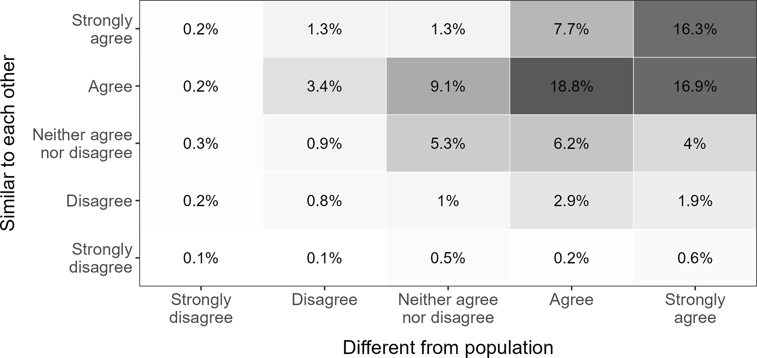
The central claim in the political class narrative is ‘the idea that members of the political class are increasingly like one another while decreasingly like the rest of the population’ (Allen Reference Allen2018: 23). To assess whether this perception is present among Danish citizens, I examine responses to two closed-ended items asking respondents how much they agree that politicians are (1) different from the population and (2) similar to each other. Figure 1 shows the cross-tabulated distribution of responses.
Distributions on political class questions.
Note: Agreement that politicians are different from the population (x-axis) and similar to each other (y-axis), with percentages in tiles. N = 1240.

A substantial majority of the respondents agree or strongly agree that politicians are a unified group of people. More concretely, 75.4% and 75.2% of the respondents agree that politicians are different from the population or similar to each other, respectively, while 59.7% agree or strongly agree with both statements. While survey respondents generally tend to agree with statements, this still suggests that many citizens perceive politicians as a socially distinct and internally homogeneous group. The question is then, what do citizens associate with this political class?
The political class in citizens’ minds
To further investigate how citizens mentally represent politicians, the following subsection presents analyses of the free association task and the open-ended responses. First, I explore the overall patterns in citizens’ conceptions of politicians before turning to how these conceptions vary depending on whether they agree that politicians constitute a socially distinct and internally homogeneous class.
Top-of-mind associations
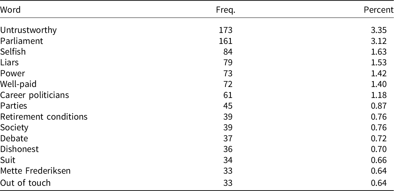
The free association task captures spontaneous, top-of-mind reactions to the cue word ‘politicians’, and Table 1 shows the 15 most frequent associations made. The first glimpse of the associations in Table 1 reveals a predominantly negative view of politicians with frequently mentioned words such as untrustworthy, selfish, and liars. However, there are likewise positive or neutral words such as society, parties, and the second most frequent word, parliament.
Most frequent responses to cue word politicians

Table 1. Long description
A table titled ‘Most frequent responses to cue word politicians’ with three columns: Word, Freq., and Percent. The table has 15 rows, each representing a different word associated with politicians. The columns are labeled ‘Word’, ‘Freq.’, and ‘Percent’. The words listed include ‘Untrustworthy’, ‘Parliament’, ‘Selfish’, ‘Liars’, ‘Power’, ‘Well-paid’, ‘Career politicians’, ‘Parties’, ‘Retirement conditions’, ‘Society’, ‘Debate’, ‘Dishonest’, ‘Suit’, ‘Mette Frederiksen’, and ‘Out of touch’. The frequencies range from 173 to 33, and the percentages range from 3.35 percent to 0.64 percent.
Note: The table shows the 15 most frequent responses for the cue word politicians. The percentage is calculated by dividing by the total number of tokens made (5158).
However, while the two most frequently mentioned terms are untrustworthy and parliament for all respondents, Table B4.1 in Appendix B4 shows that their relative frequencies are reversed when comparing respondents who endorse the political class narrative with those who do not. The most frequent association among those who perceive politicians as both internally homogeneous and socially distinct is, by far, the term untrustworthy. In contrast, the most prevalent term among those who disagree with at least one of the two statements is parliament.
Figure 2 further corroborates this by showing the distinctiveness of word usage expressed in standardised log-odds ratios. Following the approach presented in Monroe, Colaresi and Quinn (Reference Monroe, Colaresi and Quinn2017), Figure 2 depicts the words that are most distinctively used among respondents who adopt the political class narrative relative to those who do not (see also, Bisgaard Reference Bisgaard2019). The x-axis shows the logged frequency of each word in the full text corpus, while the y-axis indicates the distinctiveness of each word (expressed in z-scores). Thus, the higher the value on the y-axis, the more distinctive the word is for the group of respondents who agree that politicians are similar to each other and different from the population (and vice versa). The higher the value on the x-axis, the more frequent the term is in the overall text corpus.
Words more distinctively used among respondents agreeing/disagreeing that politicians are distinct and homogeneous.
Note: The y-axis shows a standardised log-odds ratio comparing respondents agreeing/not agreeing to both of the two closed-ended political class questions for each word occurring more than five times in the free association task. Following Monroe, Colaresi and Quinn (Reference Monroe, Colaresi and Quinn2017), the standardised log-odds ratio has been regularised with an informative Dirichlet prior (see Appendix B6 for more details). The x-axis shows the logged frequency of the word.

Several interesting patterns occur in Figure 2. First, as argued by Allen (Reference Allen2018), the political class narrative appears to be inherently negative. Words such as selfish, untrustworthy, and liars are significantly more distinctive among respondents who perceive politicians as a distinct and homogeneous class. Conversely, more neutral terms (e.g., parliament), or even positive terms (e.g., good), are more common among those who do not endorse this view of politicians. Second, among the most distinctive words used by respondents adopting the political class narrative are career politicians, out of touch, and lacking (most often used in the context of lacking work experience). This fits well with an emerging literature on the increased professionalisation of politics and the emergence of the frequently disdained career politician (Warncke, Searing and Allen Reference Warncke, Searing and Allen2024; Wright Reference Wright2013). These politicians are often reproached for lacking extra-political experience and understanding of ordinary citizens – messages that have become a recurring theme in populist appeals (Warncke, Searing and Allen Reference Warncke, Searing and Allen2024, see also Allen Reference Allen2018; Fawcett and Corbett Reference Fawcett and Corbett2018; Valgarðsson, Jennings, et al. Reference Valgarðsson, Jennings, Stoker, McKay, Devine and Clarke2025). Interestingly, however, the term highly educated is relatively more prevalent among respondents who do not agree with the political class narrative. This suggests that – even among those who reject the idea of a homogeneous political class – there exists a common conception of politicians as possessing higher levels of education. Elite attributes such as educational attainment are thus widely associated with politicians, regardless of whether respondents view them as a distinct and homogeneous class.
Figures B5.1 and B5.2 in Appendix B5 further suggest that the observed differences in respondents’ spontaneous reactions are primarily driven by perceptions of social distinctiveness. While associations made by respondents who perceive politicians as internally homogeneous closely mirror word usage among those who disagree with both statements, respondents who agree that politicians are socially distinct (or agree to both statements) use negative words more distinctively.
Open-ended questions
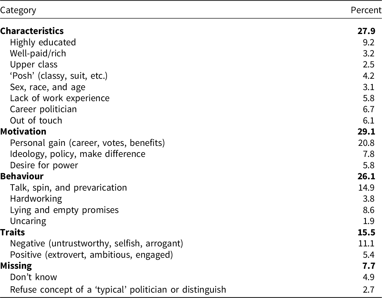
To more directly study what citizens believe characterises politicians, I supplemented the free association task with an open-ended question asking respondents how they would ‘describe a typical politician’. The responses are manually coded as stated in the methods section, and Table 2 shows the overall results of this coding.
Descriptions of ‘typical’ politicians

Table 2. Long description
The table categorizes and quantifies characteristics, motivations, behaviors, and traits of typical politicians. It has two columns: Category and Percent. The table includes the following rows: Characteristics (27.9 percent): Highly educated (9.2 percent), Well-paid/rich (3.2 percent), Upper class (2.5 percent), ‘Posh’ (classy, suit, etc.) (4.2 percent), Sex, race, and age (3.1 percent), Lack of work experience (5.8 percent), Career politician (6.7 percent), Out of touch (6.1 percent); Motivation (29.1): Personal gain (career, votes, benefits) (20.8 percent), Ideology, policy, make difference (7.8 percent), Desire for power (5.8 percent); Behaviour (26.1 percent): Talk, spin, and prevarication (14.9 percent), Hardworking (3.8 percent), Lying and empty promises (8.6 percent), Uncaring (1.9 percent). Traits (15.5 percent): Negative (untrustworthy, selfish, arrogant) (11.1 percent), Positive (extrovert, ambitious, engaged) (5.4 percent); Missing (7.7 percent): Don’t know (4.9 percent), Refuse concept of a ‘typical’ politician or distinguish (2.7 percent).
Note: N = 1238. The table shows percentages of respondents who mention a given category excluding respondents who provided no or meaningless answers such as ‘–’ (N = 64). The categories are not mutually exclusive, and hence the percentages does not sum to 100.
First, it is worth noting that the share of respondents who refused to accept the concept of a typical politician or, contrary to the question’s instructions, distinguished between politicians (e.g., by describing two types of politicians) is relatively low (2.7%). While this may be an artefact of the question suggesting that there exists such a thing as a typical politician – thus requiring respondents to actively argue against the premise of the question – it nevertheless underpins the results in Figure 1 and provides some evidence that most people hold a conception of a ‘typical’ politician. Second, the most frequent theme in the descriptions is politicians’ motivation (29.1%), with personal gain far the most dominant (20.8%). However, in line with the top-of-mind associations, mentions of career politicians (or characteristics commonly ascribed to them, that is, being out of touch and lacking work experience) feature prominently in the open-ended responses (18.6%). This, along with the high prevalence of references to politicians’ negative traits and personal motivations, fits well with the political class narrative, which depicts politicians as a homogeneous class increasingly distant from the public.
Figure 3 builds on this as well as the findings from the free association task. From this figure, it appears that the tendency to describe a typical politician as having a long political career without real-world working experience is more prevalent among the group of respondents adopting the political class narrative. Additionally, references to negative features, such as being driven by personal gain or general negative traits, are significantly more frequent among this subgroup of respondents. Conversely, the positive subcodes, such as hardworking and positive traits, are more frequently mentioned by respondents who do not perceive politicians as socially distinct and internally homogeneous. However, in contrast to the previous analysis, the share of respondents mentioning politicians’ advantageous socio-economic background is not distinguishable between the two groups. While politicians’ higher levels of education are top-of-mind for individuals who do not perceive politicians as a distinct and homogeneous group, this is commonly agreed upon when a bit more structure is provided to respondents’ thinking.
Descriptions of a ‘typical’ politician across respondents agreeing/disagreeing that politicians are distinct and homogeneous.
Note: The plot shows the percentage of respondents in each subgroup mentioning the different features in their descriptions of a typical politician. The percentages are calculated excluding respondents who provided no meaningful answer (such as ‘–’). N = 1238. *p < 0.05, **p < 0.01, ***p < 0.001.

Again, however, the fine-grained analysis using the four-category measure of endorsement of the political class narrative in Figure 4 suggests that the more consequential dimension is that concerning the social distinctiveness of the political class. For respondents who agree that politicians are similar to each other but disagree that they are different from the population, there are no significant differences in how they describe a typical politician (panel A). However, respondents who perceive politicians as distinct from the population differ significantly in their descriptions of a typical politician compared to those who disagree with both questions. For example, respondents who perceive politicians as different from the population (but not similar to each other) are significantly more likely to make references to a typical politician’s detachment from reality, describing them as out of touch and lacking work experience. These differences are further amplified when examining respondents who agree with both questions (panel C).
Descriptions of a ‘typical’ politician across four subgroups.
Note: The plot shows the difference in percentage mentioning each feature in their descriptions of a typical politician. Respondents who disagree with both statements are compared to respondents who agree that politicians are (a) similar to each other but not different from the population, (b) different from the population but not similar to each other, and (c) both similar to each other and different from the population. *p < 0.05, **p < 0.01, ***p < 0.001.

Figure 4. Long description
The image contains three sets of vertical bar graphs labeled A, B, and C, each representing different perceptions of politicians. Each set is further divided into four categories: Traits, Motivations, Behavior, and Characteristics. The horizontal axis represents the difference in percentage compared to disagreeing on both statements, ranging from -0.2 to 0.2. The vertical axis lists specific traits, motivations, behaviors, and characteristics. Panel A shows perceptions when respondents agree on similar traits, Panel B shows perceptions when respondents agree on different traits, and Panel C shows perceptions when respondents agree on both similar and different traits. Each bar graph includes markers indicating statistical significance levels: one asterisk for p < 0.05, two asterisks for p < 0.01, and three asterisks for p < 0.001. Notable trends include significant differences in perceptions of negative traits, personal motivation, lying and empty promises, and being out of touch in various panels.
Implications for political support
The final analysis of this paper examines how perceptions of the political class relate to citizens’ broader attitudes towards democracy and political institutions. Specifically, I included three measures of political support in the survey. First, I measure trust in politicians by asking respondents to indicate on a single scale ranging from 0 to 10, how much they trust politicians. Second, using the same scale, I ask respondents how satisfied they are with the way the Danish democracy is functioning. Both measures are scaled from 0 to 1, with higher values indicating more trust/satisfaction (mean ${_{trust}} = 0.37$, SD
 ${_{trust}} = 0.24$; mean
 ${_{satisfaction}} = 0.57$, SD
 ${_{satisfaction}} = 0.25$). Finally, I measure external political efficacy using three questions asking respondents to indicate how much they agree that 1) politicians consistently take voters’ opinions into account, 2) politicians are only interested in my vote, not my opinions (reversed) and 3) people like me have no influence on the policies pursued (reversed). Respondents could answer on a scale from 1 (completely disagree) to 5 (completely agree). Answers to these questions are combined into a single measure of external political efficacy, which is scaled from 0 to 1 with higher values indicating a greater sense of efficacy (
 $\alpha = 0.72$, mean
 $= 0.36$, SD
 $= 0.22$).
To study how citizens’ mental representations of politicians relate to their level of political support, I run regression models, with each measure of political support as the dependent variable and categorical variables constructed – as described above – based on respondents’ answers to the two closed-ended questions regarding politicians’ internal homogeneity and social distinctiveness as independent variables. Additionally, I adjust for respondents’ sex, age, education, income, and subjective social class (for the full regression tables, see Appendix D).
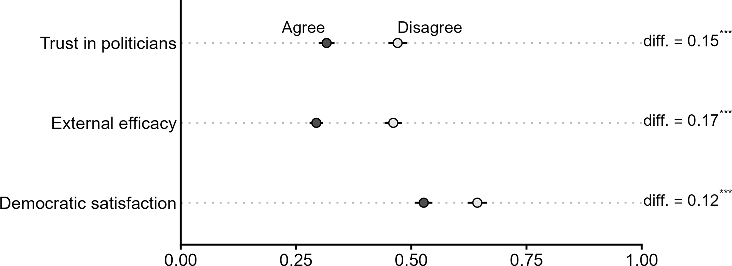
Unsurprisingly, Figure 5 shows that perceiving politicians as both socially distinct and internally homogeneous is associated with significantly lower levels of political support compared to those respondents who disagree with at least one of the statements. Specifically, respondents who perceive politicians as both similar to each other and different from the population report significantly lower levels of trust in politicians ( $\! - 15$ % points), external political efficacy (
 $\! - 17$ % points), and democratic satisfaction (
 $\!- 12$ % points) compared to those who reject the narrative. While the analysis is based on observational data – thus precluding any strict causal interpretation – it does indicate support for the notion that perceiving politicians as ‘all the same’ and ‘out-of-touch’ may be an important underlying explanation for contemporary patterns of political dissatisfaction (see Valgarðsson, Jennings, et al. Reference Valgarðsson, Jennings, Stoker, McKay, Devine and Clarke2025; Valgarðsson, Clarke, et al. Reference Valgarðsson, Clarke, Jennings and Stoker2021).
Predicted levels of political support across agreeing/disagreeing respondents.
Note: The plot shows the estimated political support for respondents who agree that politicians are both similar to each other and different from the population (dark grey) and respondents who disagree with at least one of the two closed-ended political class questions (light grey). The estimates are derived from three regression models adjusting for respondents’ sex, age, education, income, and subjective social class (for the full regression table, see Appendix D1). N = 1099.

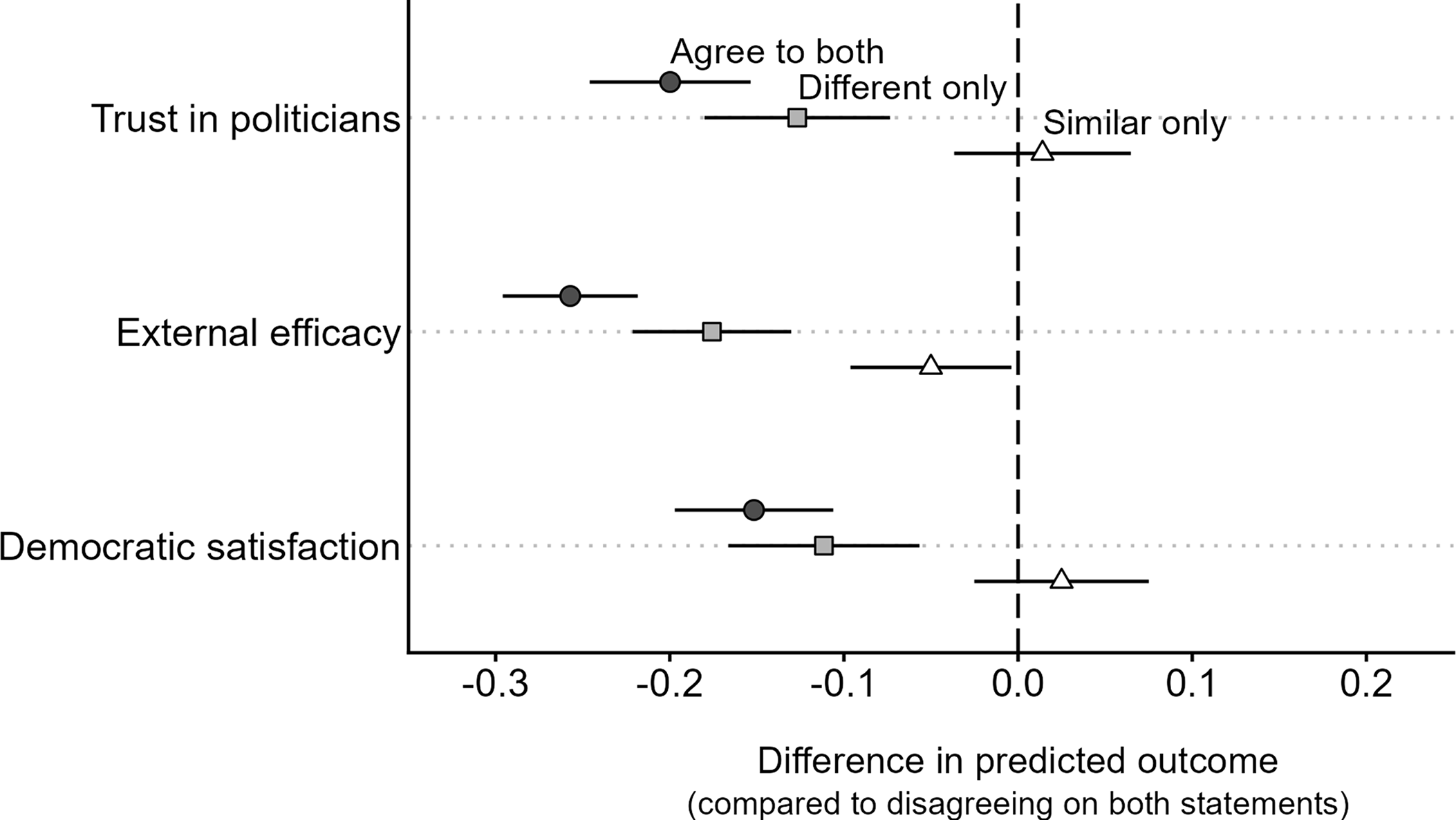
However, while the narrative of an internally homogeneous and socially distinct political class is intimately related to lower levels of political support, it appears from Figure 6 that the latter dimension concerning the social distinctiveness is the more consequential one. This figure – using the more fine-grained categorisation that separates the two dimensions – shows that the negative association with lower levels of political support is more pronounced among respondents who view politicians as different from the general population. In contrast, when comparing the similar-only category with respondents who disagree with both statements, there are no meaningful differences in levels of political support. Perceiving the group of politicians as internally homogeneous may thus constitute less of a problem for democratic legitimacy, as long as this group is not viewed as different from the rest of the population. Conversely, perceiving politicians as socially distinct from the general population is associated with significantly lower levels of political trust, external efficacy, and democratic satisfaction, regardless of whether one also perceives them as internally homogeneous.
Difference in predicted outcome.
Note: The plot shows the difference in predicted outcomes comparing respondents who disagree with both political class questions with respondents agreeing that politicians are internally homogeneous (white triangles), different from the population (grey squares) and both questions (dark grey circles). The estimates are derived from three regression models adjusting for respondents’ sex, age, education, income, and subjective social class (for the full regression table, see Appendix D2). N = 1099.

Conclusion
The narrative portraying politicians as socially distinct and internally homogeneous is a recurring theme in contemporary political discourse. However, while this may provide a straightforward and intuitively appealing explanation for recent patterns of rising political discontent, its empirical grounding in the public remains underexplored. Existing research has largely focused on the objective characteristics of elected officials, the rhetorical strategies employed by political elites, or whether citizens adopt a populist worldview. Drawing on original survey data from Denmark – a context characterised by relatively high descriptive representation and a large number of diverse political parties – this study shifts the analytical focus to the public’s mental representations, examining how citizens themselves perceive the group of politicians.
Using a combination of free association tasks, open-ended descriptions, and closed-ended items, I show that a substantial share of voters perceive politicians as a unified group, distinct from the general population and similar to one another. These mental representations are not only widespread but also consequential. Citizens who endorse the political class narrative are more likely to associate and describe politicians with negative traits and characteristics, such as being out of touch and lacking job experience outside politics. Moreover, perceiving politicians as socially distinct and internally homogeneous is systematically linked to lower levels of political trust, external efficacy, and democratic satisfaction. This suggests that mental representations of the political class may play a significant role in shaping democratic attitudes, even in contexts with comparatively high elite diversity. Importantly, the findings further suggest that it is the perception of social distinctiveness – rather than internal homogeneity – that is most strongly connected to negative evaluations of politicians and diminished democratic support. Citizens who view politicians as fundamentally different from the population are more likely to associate them with negative traits such as selfishness, dishonesty, and detachment from everyday life.
By shifting the analytical focus to citizens’ mental representations, this study contributes to a growing literature on political representation and democratic attitudes. The use of free associations and open-ended descriptions contributes to a deeper understanding of the cognitive underpinnings of contemporary political discontent in ways that are not easily captured by existing research. Additionally, it goes beyond populist attitude scales by examining how citizens categorise politicians as a distinct, homogeneous group, and how these dimensions of the political class narrative – both together and individually – relate to broader democratic attitudes. The study thus highlights the need to understand how voters mentally construct the category of ‘politicians’, suggesting that democratic legitimacy depends not only on who politicians are but also on how they are imagined by the public.
However, while the multi-method approach undertaken here offers a rich understanding of how citizens mentally represent the political class and the content of those representations, it comes with two important drawbacks. First, the approach taken in this paper does not allow for causal inference. The observed associations between perceptions of a political class and broader measures of political support should therefore not be interpreted as establishing that such perceptions cause lower trust or satisfaction. Future research could address this limitation using designs better suited to identifying causal effects. For example, building on Valgarðsson, Jennings, et al. (Reference Valgarðsson, Jennings, Stoker, McKay, Devine and Clarke2025), conjoint experiments could examine how traits that deviate from the perceived political class shape evaluations of individual politicians, while vignette experiments manipulating, for example, perceived parliamentary class composition could address how parliamentary (class) diversity shapes broader institutional trust and satisfaction – and indeed whether this translates into more concrete demands for more diverse parliaments.
Second, the findings raise a broader question about the origins of citizens’ mental representations of the political class, which cross-sectional data cannot address. While Denmark is often considered a comparatively inclusive case in terms of descriptive representation, important representation gaps remain with regard to, for example, social class and ethnic background. These gaps may contribute to the perceived social distinctiveness of politicians, but the present analysis cannot determine the extent to which citizens’ perceptions of the political class accurately reflect these patterns. While mental representations of politicians may be shaped by objective representational gaps, media commentary, or political discourse, the research design employed here cannot assess these influences. Future work should examine this using, for example, longitudinal data that track both mental representations of politicians and changes in the social composition of parliaments or in dominant media narratives.
Overall, the findings suggest that politicians constitute a unique social category in the minds of voters. Once individuals enter the realm of formal politics, they may – simply by the virtue of being a politician – be cognitively reclassified in ways that diminish their perceived proximity to ordinary citizens. Addressing contemporary patterns of rising political discontent, therefore, may require more than diversifying who holds office. It demands a deeper engagement with how politicians are imagined, categorised, and evaluated by the public.
Supplementary material
The supplementary material for this article can be found at https://doi.org/10.1017/S1475676526101777
Data availability statement
Replication materials are available at https://doi.org/10.7910/DVN/DYZ1P7
Acknowledgements
I am grateful to the anonymous reviewers and the editors for their valuable comments and thoughtful suggestions, which helped improve the manuscript. Additionally, I wish to thank Rune Stubager, Martin Bisgaard, Tim Lars Allinger, Emil Bories Hüttel, and Larissa Böckmann for their helpful comments and feedback.
Financial support
This research was supported by Aarhus University, Department of Political Science.
Competing interests
None to disclose.
Ethical standards
The study does not raise ethical concerns. It complies with national regulations and professional guidelines for studying human subjects and follows data protection regulations. According to Danish national regulations, the study was exempt from formal IRB review (see Online Appendix E for ethical considerations).
Use of AI
Generative AI tools (Claude) were used for language improvement and for coding assistance related to R-based plot editing. After using this tool, the author reviewed and edited the content as needed and takes full responsibility for the content of the publication.





 Open access

