2.1. Two-phase Stokes system

We are interested in the quasi-static evolution of multiple clean droplets in an incompressible flow. The droplets experience no phase change, but are driven by a constant surface tension at the fluid–fluid interface. Such a system is governed by the two-phase Stokes equations, which have been described in detail in classic monographs (see Ladyzhenskaya Reference Ladyzhenskaya1963; Pozrikidis Reference Pozrikidis1992; Temam Reference Temam2001). The notation and main auxiliary results used below are presented in appendix A.

We consider a three-dimensional domain $\varOmega _- \subset \mathbb {R}^d, d = 3$, and its complement $\varOmega _+ = \mathbb {R}^d \setminus \bar {\varOmega }_-$ to denote the union of the droplets’ interiors and the ambient fluid, respectively. The boundary between the two domains is $\varSigma \triangleq \bar {\varOmega }_- \cap \bar {\varOmega }_+$. In the following, we assume $\varSigma$ is a finite set of disjoint, closed, bounded and orientable surfaces. Furthermore, we require that $\varSigma$ is of class $\mathcal {C}^2$ to allow for the definition of a unique curvature at every point.

The droplets and the ambient fluid have dynamic viscosities $\mu _-$ and $\mu _+$, respectively. The flow in each phase is described by the velocity fields $\boldsymbol {u}_\pm : \varOmega _\pm \to \mathbb {R}^d$ and the pressures $p_\pm : \varOmega _\pm \to \mathbb {R}$. We also define the Cauchy stress tensor and the rate-of-strain tensor by

(2.1)\begin{equation} \left.\begin{array}{c@{}} \sigma_\pm \triangleq -p_\pm {\boldsymbol{\mathsf{I}}} + 2 \mu_\pm \varepsilon_\pm, \\ \varepsilon_\pm \triangleq \tfrac{1}{2} (\boldsymbol{\nabla} \boldsymbol{u}_\pm + (\boldsymbol{\nabla} \boldsymbol{u}_\pm)^T). \end{array}\right\} \end{equation}

Following these definitions, the static incompressible two-phase Stokes equations are given by

(2.2)\begin{equation} \left.\begin{array}{c@{}} \boldsymbol{\nabla} \boldsymbol{\cdot} \boldsymbol{u}_\pm = 0, \quad \boldsymbol{x} \in \varOmega_\pm, \\ \boldsymbol{\nabla} \boldsymbol{\cdot} \sigma_\pm = 0, \quad \boldsymbol{x} \in \varOmega_\pm, \\ \boldsymbol{u}_+ = \boldsymbol{u}^\infty, \quad \|\boldsymbol{x}\| \to \infty. \end{array}\right\} \end{equation}

The boundary conditions at the interface between the fluids are given as a set of jump conditions on $\varSigma$. Namely, the velocity must satisfy a no-slip condition and the surface stresses are related to the additive curvature of the interface by the Young–Laplace law. We write

(2.3)\begin{equation} \left.\begin{array}{c@{}} {[\![ \boldsymbol{u} ]\!]} = 0, \\ {[\![\, \boldsymbol{f} ]\!]} = \gamma \kappa \boldsymbol{n},\end{array}\right\} \end{equation}

where $\boldsymbol {f}_\pm \triangleq \boldsymbol {n} \boldsymbol {\cdot } \sigma _\pm$ is the surface traction, $\gamma$ is the surface tension coefficient and $\boldsymbol {n}$ is the exterior normal vector to $\varOmega _-$. The jump operator is defined as $[\![\, f ]\!] \triangleq f_+(\boldsymbol {x}_+) - f_-(\boldsymbol {x}_-)$, where

(2.4)\begin{equation} f(\boldsymbol{x}_\pm) = \lim_{\epsilon \to 0^+} \boldsymbol{f}(\boldsymbol{x} \pm \epsilon \boldsymbol{n}). \end{equation}

It is convenient to non-dimensionalize the equations to reduce the number of parameters in the problem. We choose the following non-dimensionalizations, common in the literature:

(2.5a–c)\begin{equation} \boldsymbol{u}_\pm = U \hat{\boldsymbol{u}}_\pm, \quad p_\pm = \frac{\mu_\pm U}{R} \hat{p}_\pm, \quad \boldsymbol{x} = R \hat{\boldsymbol{x}}, \end{equation}

where $U$ is a characteristic velocity magnitude and $R$ is a characteristic droplet radius. The resulting non-dimensional parameters governing the systems are the viscosity ratio $\lambda$ and the capillary number $\textit {Ca}$, defined as

(2.6a,b)\begin{equation} \lambda \triangleq \frac{\mu_-}{\mu_+} \quad \text{and} \quad \textit{Ca} \triangleq \frac{\mu_+ U}{\gamma}. \end{equation}

In the remainder, we will continue by using the non-dimensional equations. We will write the non-dimensional stress jump condition (2.3) as follows:

(2.7)\begin{equation} [\![\, \boldsymbol{f} ]\!] _\lambda \triangleq \boldsymbol{f}_+ - \lambda \boldsymbol{f}_- = \frac{1}{\textit{Ca}} \kappa \boldsymbol{n}. \end{equation}

In order to evolve the shape of the droplets in time, we use a quasi-static approach in which we first compute the velocity using (2.2) and then displace the interface using an ordinary differential equation. The evolution of the interface is described by

(2.8)\begin{equation} \dfrac{\partial \boldsymbol{X}}{\partial \tau} = \boldsymbol{V}(\boldsymbol{u}, \boldsymbol{X}), \end{equation}

where $\boldsymbol {X}$ is a parameterization of the interface and $\boldsymbol {V}$ is a given source term. Typical examples of the source term are

(2.9)\begin{equation} \boldsymbol{V}(\boldsymbol{u}, \boldsymbol{X}) \triangleq (\boldsymbol{u} \boldsymbol{\cdot} \boldsymbol{n}) \boldsymbol{n} + ({\boldsymbol{\mathsf{I}}} - \boldsymbol{n} \otimes \boldsymbol{n}) \boldsymbol{w}, \end{equation}

where $\boldsymbol {w}$ can be chosen to be $\boldsymbol {0}, \boldsymbol {u}$ or a different tangential correction to $\boldsymbol {u}$. The choice of $\boldsymbol {w}$ is left open, since only the normal component of the velocity field governs the deformation of the interface. The tangential component can be artificially imposed for numerical reasons, e.g. to cluster points in regions of high curvature; for example, see the works of Hou et al. (Reference Hou, Lowengrub and Shelley1994) and Ojala & Tornberg (Reference Ojala and Tornberg2015).

2.2. Shape derivatives

Interfacial control in multiphase flows with sharp interfaces is inherently a form of shape optimization. With this in mind, we will review some of the concepts behind shape optimization and perturbations with respect to the domain. We consider here Hadamard's method for boundary variations, which has been detailed rigorously in works such as Moubachir & Zolésio (Reference Moubachir and Zolésio2006), Allaire & Schoenauer (Reference Allaire and Schoenauer2007), Delfour & Zolésio (Reference Delfour and Zolésio2001) and, from the view of differential geometry, in Walker (Reference Walker2015).

The method is based on defining so-called perturbations of the identity by

(2.10)\begin{equation} \varOmega_\epsilon = \boldsymbol{X}_\epsilon(\varOmega) = (\mathrm{Id} + \epsilon \tilde{\boldsymbol{X}})(\varOmega), \end{equation}

where $\mathrm {Id}$ is the identity mapping, $\tilde {\boldsymbol {X}} \in W^{2, \infty }(\mathbb {R}^d; \mathbb {R}^d)$ is a perturbation and $\epsilon > 0$ is a real constant. If $\epsilon$ is sufficiently small, then $\boldsymbol {X}_\epsilon$ is a diffeomorphism on $\mathbb {R}^d$ (Allaire & Schoenauer Reference Allaire and Schoenauer2007, lemma 6.13). As such, by Hadamard's method we can identify every admissible shape $\varOmega _\epsilon$ with a perturbation $\boldsymbol {X}_\epsilon$. Therefore, the method allows, among other things, defining differentiation of shapes by differentiation in the Banach space $W^{2, \infty }(\mathbb {R}^d; \mathbb {R}^d)$ in terms of well known concepts, such as the Gâteaux and Fréchet derivatives.

In fact, using this simple definition, we can define the Fréchet derivatives of relevant functionals of the type

(2.11)\begin{equation} \left.\begin{array}{c@{}} \displaystyle\mathcal{J}_1(\varOmega) \triangleq \int_{\varOmega} f(\boldsymbol{x}; \varOmega)\, \textrm{d} V, \\ \displaystyle\mathcal{J}_2(\varSigma) \triangleq \int_{\varSigma} f(\boldsymbol{x}; \varOmega) \,{\rm d}S, \\ \displaystyle\mathcal{J}_3(\varSigma) \triangleq \int_{\varSigma} g(\boldsymbol{x}; \varSigma) \,{\rm d}S. \end{array}\right\} \end{equation}

We refer to Allaire & Schoenauer (Reference Allaire and Schoenauer2007) and Walker (Reference Walker2015) for proofs of these results and additional shape derivatives of quantities of interest, such as the normal and the additive curvature. The lemma below reproduces the main derivatives of functionals used in the current work.

Lemma 2.1 ( Walker Reference Walker2015, lemma 5.7)

Let $\tilde {\boldsymbol {X}} \in W^{2, \infty }(\mathbb {R}^d; \mathbb {R}^d)$ be a sufficiently small perturbation, $\varOmega \subset \mathbb {R}^d$ and $\varSigma \subset \mathbb {R}^d$ a $d - 1$ manifold without boundary. Then, we have that the shape derivatives of the functionals (2.11) are

(2.12)\begin{equation} \left.\begin{array}{c@{}} \displaystyle D \mathcal{J}_1[\tilde{\boldsymbol{X}}] = \int_\varOmega f'[\tilde{\boldsymbol{X}}] + \int_{\partial \varOmega} f \tilde{\boldsymbol{X}} \boldsymbol{\cdot} \boldsymbol{n} \, {\rm d} S, \\ \displaystyle D \mathcal{J}_2[\tilde{\boldsymbol{X}}] = \int_\varSigma f'[\tilde{\boldsymbol{X}}] + \int_{\varSigma} (\boldsymbol{\nabla} f \boldsymbol{\cdot} \boldsymbol{n} + \kappa f) \tilde{\boldsymbol{X}} \boldsymbol{\cdot} \boldsymbol{n} \, {\rm d} S, \\ \displaystyle D \mathcal{J}_3[\tilde{\boldsymbol{X}}] = \int_\varSigma g'[\tilde{\boldsymbol{X}}] + \int_{\varSigma} \kappa g \tilde{\boldsymbol{X}} \boldsymbol{\cdot} \boldsymbol{n} \, {\rm d} S. \end{array}\right\} \end{equation}

Extensions to moving domains $\varOmega (t)$ and $\varSigma (t)$ are presented in Moubachir & Zolésio (Reference Moubachir and Zolésio2006). An important result in shape optimization is the Hadamard–Zolésio structure theorem from Delfour & Zolésio (Reference Delfour and Zolésio2001, theorem 3.6, chapter 9), which guarantees that we can always express the first-order shape derivative of functionals (2.11) as boundary integrals that only depend on the normal component of $\tilde {\boldsymbol {X}}$. Restricting the shape gradient to the boundary of a domain $\varOmega$ is of special interest to us, since it greatly simplifies the numerical aspects. In particular, it allows restricting the whole problem to a problem on the interface $\varSigma$ between the droplets and the surrounding fluid.

Finally, we will informally consider the shape differentiability of surface functionals that depend on the problem variables $p_\pm , \boldsymbol {u}_\pm$ and $\boldsymbol {X}$. The main issue, also discussed in Pantz (Reference Pantz2005) and Allaire et al. (Reference Allaire, Jouve and van Goethem2011), is that $\boldsymbol {u}$ as a function on $\varOmega$ is not shape differentiable, but $\boldsymbol {u}_\pm$ as restrictions to $\varOmega _\pm$ are shape differentiable.

Recall that, for $\textit {Ca} < \infty$, there is always a non-zero jump in pressure

(2.13)\begin{equation} [\![ p ]\!] = (1 - \lambda) (\boldsymbol{n} \boldsymbol{\cdot} \boldsymbol{\nabla} \boldsymbol{u}) \boldsymbol{\cdot} \boldsymbol{n} + \frac{1}{\textit{Ca}} \kappa, \end{equation}

and the following jumps in the components of the velocity gradient

(2.14a–c)\begin{equation} [\![ \boldsymbol{t}^\alpha \boldsymbol{\cdot} \boldsymbol{\nabla} \boldsymbol{u} ]\!] = 0, \quad [\![ \boldsymbol{n} \boldsymbol{\cdot} \boldsymbol{\nabla} \boldsymbol{u} ]\!] \ne 0 \quad \text{and} \quad [\![ (\boldsymbol{n} \boldsymbol{\cdot} \boldsymbol{\nabla} \boldsymbol{u}) \boldsymbol{\cdot} \boldsymbol{n} ]\!] = 0, \end{equation}

where $\boldsymbol {t}^\alpha$, for $\alpha \in \{1, \ldots , d - 1\}$, is an orthonormal basis for the tangent space to $\varSigma$. Similar jump relations can be derived for the rate-of-strain tensor. With this in mind, we consider the general functional

(2.15)\begin{equation} \mathcal{J} = \int_\varSigma j(p_\pm, \boldsymbol{u}, \boldsymbol{X}) \,{\rm d}S. \end{equation}

We can see from lemma 2.1 that the integrand must be differentiable up to the boundary to allow defining $\boldsymbol {\nabla } j \boldsymbol {\cdot } \boldsymbol {n}$. In the following, we will restrict to differentiable functionals of the type

(2.16)\begin{equation} \mathcal{J} = \int_\varSigma j(\boldsymbol{u} \boldsymbol{\cdot} \boldsymbol{n}, \boldsymbol{X}) \,{\rm d}S, \end{equation}

i.e. that only depend on the normal component of the velocity field and the surface parameterization, both of which have continuous normal gradients. In the case of volume integrals, we would not need further restrictions on the cost functionals we consider.

3.1. Static problem

We start by looking at the optimization problem (P1) with the static constraints (2.2) and (2.3). The resulting Lagrangian can be written as

(3.5)\begin{equation} \mathscr{L}_1 \triangleq \mathscr{J}_1 - \langle \boldsymbol{z}^*, \mathscr{E}_1(\boldsymbol{w}, \boldsymbol{X}) \rangle, \end{equation}

where $\boldsymbol {z}^*$ are the adjoint variables and $\boldsymbol {w}_\pm \triangleq (\boldsymbol {u}_\pm , p_\pm )$ are the state variables on $\varOmega _\pm$, such that $\boldsymbol {w} \triangleq (\boldsymbol {w}_+, \boldsymbol {w}_-)$. Expanding the constraints, we write

(3.6)\begin{align} \mathscr{L}_1 &\triangleq \mathscr{J}_1 + \int_{\varOmega_+} \boldsymbol{\nabla} \boldsymbol{u}^*_+ \boldsymbol{\cdot} \sigma_+ \, \textrm{d} V - \int_{\varOmega_+} p^*_+ (\boldsymbol{\nabla} \boldsymbol{\cdot} \boldsymbol{u}_+)\, \textrm{d} V + \frac{1}{\textit{Ca}} \int_\varSigma \kappa \langle \boldsymbol{u}^* \rangle \boldsymbol{\cdot} \boldsymbol{n} \, {\rm d} S \nonumber\\ &\quad + \int_{\varOmega_-} \lambda \boldsymbol{\nabla} \boldsymbol{u}^*_- \boldsymbol{\cdot} \sigma_- \, \textrm{d} V - \int_{\varOmega_-} \lambda p^*_- (\boldsymbol{\nabla} \boldsymbol{\cdot} \boldsymbol{u}_-)\, \textrm{d} V \nonumber\\ &\quad + \int_\varSigma \langle \,\boldsymbol{f} \rangle _\lambda \boldsymbol{\cdot} [\![ \boldsymbol{u}^* ]\!] \, {\rm d} S + \int_\varSigma \langle \,\boldsymbol{f}^* \rangle _\lambda \boldsymbol{\cdot} [\![ \boldsymbol{u} ]\!] \, {\rm d} S, \end{align}

where $\langle \,f \rangle _\lambda$ denotes a weighted average, defined as

(3.7)\begin{equation} \langle \,f \rangle _\lambda \triangleq \tfrac{1}{2} (f_+ + \lambda f_-). \end{equation}

The weak form of the Stokes equations, (2.2), can be obtained by integration by parts and then applying the following equality:

(3.8)\begin{equation} [\![\, f g ]\!] _\lambda = [\![\, f ]\!] \langle g \rangle _\lambda + \langle \,f \rangle [\![ g ]\!] _\lambda. \end{equation}

Remark 3.3 The main subtlety in our derivation comes from the choice in constructing the Lagrangian. In classic single-phase works, such as Bewley, Moin & Temam (Reference Bewley, Moin and Temam2001) and Wei & Freund (Reference Wei and Freund2006), the strong form of the equations is used with an integral over the whole domain. In the context of multiphase flows, such an approach would be possible using the one-fluid model, where $(\boldsymbol {u}, p)$ are considered as bulk variables with the jump conditions carried over as singular source terms. However, such a choice results in an incorrect shape derivative. As discussed in Pantz (Reference Pantz2005), the reason for this is that the state variables are not shape differentiable over $\varOmega$.

Therefore, equations with discontinuous coefficients and, in particular, multiphase flows must be treated with care. The correct construction involves considering the restrictions to $\varOmega _\pm$, i.e. $(\boldsymbol {u}_\pm , p_\pm )$ as above, and enforcing values that are well-defined on the interface. For example, an alternative expansion of

(3.9)\begin{equation} [\![\, f g ]\!] _\lambda = f_+ [\![ g ]\!] _\lambda + \lambda [\![\, f ]\!] g_-, \end{equation}

would lead to ill-defined results. The choice of a weak form in (3.6) is not formally required, but allows us to directly apply the results from lemma 2.1 and is consistent with the methods used in the shape optimization community, e.g. in Allaire & Schoenauer (Reference Allaire and Schoenauer2007).

We start by stating the equations satisfied by the adjoint variables in the following result.

Lemma 3.4 At a stationary point of the Lagrangian (3.6), the adjoint variables $\boldsymbol {w}^*_\pm$ satisfy the following equations:

(3.10)\begin{equation} \left.\begin{array}{c@{}} \boldsymbol{\nabla} \boldsymbol{\cdot} \boldsymbol{u}^*_\pm = 0, \quad \boldsymbol{x} \in \varOmega_\pm, \\ \boldsymbol{\nabla} \boldsymbol{\cdot} \sigma^*_\pm = 0, \quad \boldsymbol{x} \in \varOmega_\pm, \\ \boldsymbol{u}^*_+ = 0, \quad \|\boldsymbol{x}\| \to \infty, \end{array}\right\} \end{equation}

with the jump conditions

(3.11)\begin{equation} \left.\begin{array}{c@{}} {[\![ \boldsymbol{u}^* ]\!]} = 0, \\ {[\![\, \boldsymbol{f}^* ]\!]} _\lambda = \boldsymbol{\nabla}_{\boldsymbol{u}} \mathcal{J}_1. \end{array}\right\} \end{equation}

The adjoint Cauchy stress tensor, rate-of-strain tensor and traction vector are in complete analogy to the definitions of the primal Stokes problem given in § 2. For the cost functional (3.1), we have that

(3.12)\begin{equation} \boldsymbol{\nabla} _{\boldsymbol{u}} \mathcal{J}_1 = (\boldsymbol{u} \boldsymbol{\cdot} \boldsymbol{n} - u_d) \boldsymbol{n}. \end{equation}

Proof. The adjoint equations are easily obtained by differentiating the Lagrangian with respect to the state variables $\boldsymbol {w}_\pm$. We have that

(3.13)\begin{align} \dfrac{\partial \mathscr{L}_1}{\partial \boldsymbol{w}} [\tilde{\boldsymbol{w}}] &= \dfrac{\partial \mathcal{J}_1}{\partial \boldsymbol{w}} [\tilde{\boldsymbol{w}}] + \int_{\varOmega_+} \boldsymbol{\nabla} \boldsymbol{u}^*_+ \boldsymbol{\cdot} \tilde{\sigma}_+ \, \textrm{d} V - \int_{\varOmega_+} p^*_+ (\boldsymbol{\nabla} \boldsymbol{\cdot} \tilde{\boldsymbol{u}}_+)\, \textrm{d} V \nonumber\\ &\quad + \int_{\varOmega_-} \lambda \boldsymbol{\nabla} \boldsymbol{u}^*_- \boldsymbol{\cdot} \tilde{\sigma}_- \, \textrm{d} V - \int_{\varOmega_-} \lambda p^*_- (\boldsymbol{\nabla} \boldsymbol{\cdot} \tilde{\boldsymbol{u}}_-)\, \textrm{d} V + \int_\varSigma \langle \,\tilde{\boldsymbol{f}} \rangle_\lambda \boldsymbol{\cdot} [\![ \boldsymbol{u}^* ]\!] \, {\rm d} S. \end{align}

For $k \in \{+, -\}$, we have that

(3.14)\begin{equation} \int_{\varOmega_k} \boldsymbol{\nabla} \boldsymbol{u}^*_k \boldsymbol{\cdot} \tilde{\sigma}_k \, \textrm{d} V - \int_{\varOmega_k} p^*_k (\boldsymbol{\nabla} \boldsymbol{\cdot} \tilde{\boldsymbol{u}}_k)\, \textrm{d} V \\ = \int_{\varOmega_k} \sigma^*_k \boldsymbol{\cdot} \boldsymbol{\nabla} \tilde{\boldsymbol{u}}_k \, \textrm{d} V - \int_{\varOmega_k} (\boldsymbol{\nabla} \boldsymbol{\cdot} \boldsymbol{u}^*_k) \tilde{p}_k \, \textrm{d} V, \end{equation}

by algebraic manipulations. This is the weak formulation of the adjoint equations from lemma 3.4 with test functions $(\tilde {\boldsymbol {u}}_\pm , \tilde {p}_\pm )$.

We are now in a position to give the definition of the shape derivative of the cost functional from (P1). It is stated as follows.

Theorem 3.5 We assume that $(\boldsymbol {u}_\pm , p_\pm )$ and $\mathscr {J}_1$ are shape differentiable. Then, the shape gradient of the cost functional (P1) is

(3.15)\begin{equation} \boldsymbol{\nabla} _{\boldsymbol{X}} \mathscr{J}_1 = \boldsymbol{\nabla} _{\boldsymbol{X}} \mathcal{J}_1 + \mathcal{C}^*[\boldsymbol{w}^*; \boldsymbol{X}] + \mathcal{S}^*[\boldsymbol{w}^*, \boldsymbol{X}, \boldsymbol{w}], \end{equation}

where

(3.16)\begin{equation} \left.\begin{array}{c@{}} \mathcal{C}^*[\boldsymbol{w}^*; \boldsymbol{X}] \triangleq \dfrac{1}{\textit{Ca}} ( \kappa^*[\boldsymbol{u}^* \boldsymbol{\cdot} \boldsymbol{n}] + n^*[\kappa \boldsymbol{u}^* \boldsymbol{\cdot} \boldsymbol{t}] + \kappa^2 \boldsymbol{u}^* \boldsymbol{\cdot} \boldsymbol{n} + \kappa (\boldsymbol{n} \boldsymbol{\cdot} \boldsymbol{\nabla} \boldsymbol{u}^*) \boldsymbol{\cdot} \boldsymbol{n} ), \\ \mathcal{S}^*[\boldsymbol{w}^*; \boldsymbol{X}, \boldsymbol{w}] \triangleq \langle \,\boldsymbol{f} \rangle _\lambda \boldsymbol{\cdot} [\![ \boldsymbol{n} \boldsymbol{\cdot} \boldsymbol{\nabla} \boldsymbol{u}^* ]\!] + \langle \,\boldsymbol{f}^* \rangle _\lambda \boldsymbol{\cdot} [\![ \boldsymbol{n} \boldsymbol{\cdot} \boldsymbol{\nabla} \boldsymbol{u} ]\!] - 2 [\![ \varepsilon^* \boldsymbol{\cdot} \varepsilon ]\!] _\lambda. \end{array}\right\} \end{equation}

For the cost functional (3.1), we have that

(3.17)\begin{equation} \boldsymbol{\nabla} _{\boldsymbol{X}} \mathcal{J}_1 = n^*[\,j \boldsymbol{u}] + j (\boldsymbol{n} \boldsymbol{\cdot} \boldsymbol{\nabla} \boldsymbol{u}) \boldsymbol{\cdot} \boldsymbol{n} + \tfrac{1}{2} \kappa j^2, \end{equation}

where $j \triangleq \boldsymbol {u} \boldsymbol {\cdot } \boldsymbol {n} - u_d$. The operators $\kappa ^*$ and $n^*$ correspond to the adjoint operators of the Eulerian shape derivative of the additive curvature and normal vector, respectively. They are defined in appendix B.

3.2. Quasi-static problem

The extension from (P1) to the unsteady problem (P2) is straightforward from the point of view of the Lagrangian formalism. However, introducing the unsteady element complicates the theoretical analysis of the problem, since it is not clear if the solution will maintain the required smoothness. Similar issues appear at a numerical level, as we will see in subsequent sections.

Furthermore, the shape derivative formalism from § 2.2 needs to be extended. Intuitively, we now want to perturb the time-dependent domains $\varOmega _\pm (t)$. In the $(d + 1)$-dimensional $(t, \boldsymbol {x})$ space, one can think of a fixed domain $\varOmega$ as a cylinder, while a moving domain $\varOmega (t)$ will be a general tubular manifold. Domain perturbations of this kind were made rigorous in Moubachir & Zolésio (Reference Moubachir and Zolésio2006), to which we refer to any additional details.

As before, the Lagrangian functional associated with (P2) is given by

(3.18)\begin{equation} \mathscr{L}_2 \triangleq \mathscr{J}_2 - \langle \boldsymbol{z}^*, \mathscr{E}_2(\boldsymbol{w}, \boldsymbol{X}, \textit{Ca}) \rangle, \end{equation}

or, explicitly,

(3.19)\begin{align} \mathscr{L}_2 &\triangleq \mathscr{J}_2 + \int_0^T \int_{\varOmega_+(t)} \boldsymbol{\nabla} \boldsymbol{u}^*_+ \boldsymbol{\cdot} \sigma_+ \, \textrm{d} V \, \textrm{d} t - \int_0^T \int_{\varOmega_+(t)} p^*_+ (\boldsymbol{\nabla} \boldsymbol{\cdot} \boldsymbol{u}_+)\, \textrm{d} V \, \textrm{d} t \nonumber\\ &\quad + \int_0^T \int_{\varOmega_-(t)} \lambda \boldsymbol{\nabla} \boldsymbol{u}^*_- \boldsymbol{\cdot} \sigma_- \, \textrm{d} V \, \textrm{d} t - \int_0^T \int_{\varOmega_-(t)} \lambda p^*_- (\boldsymbol{\nabla} \boldsymbol{\cdot} \boldsymbol{u}_-)\, \textrm{d} V \, \textrm{d} t \nonumber\\ &\quad + \frac{1}{\textit{Ca}} \int_0^T \int_{\varSigma(t)} \kappa \boldsymbol{u}^* \boldsymbol{\cdot} \boldsymbol{n} \, {\rm d} S \, \textrm{d} t \nonumber\\ &\quad + \int_0^T \int_{\varSigma(t)} \langle \,\boldsymbol{f} \rangle _\lambda \boldsymbol{\cdot} [\![ \boldsymbol{u}^* ]\!] \, {\rm d} S \, \textrm{d} t + \int_0^T \int_{\varSigma(t)} \langle \,\boldsymbol{f}^* \rangle _\lambda \boldsymbol{\cdot} [\![ \boldsymbol{u} ]\!] \, {\rm d} S \, \textrm{d} t \nonumber\\ &\quad - \int_0^T \int_{\varSigma(t)} \boldsymbol{X}^* \boldsymbol{\cdot} (\boldsymbol{X}_t - \boldsymbol{V}(\boldsymbol{u}, \boldsymbol{X})) \,{\rm d}S \, \textrm{d} t \nonumber\\ & \quad -\int_{\varSigma(0)} \boldsymbol{X}^*_0 \boldsymbol{\cdot} (\boldsymbol{X}(0) - \boldsymbol{X}_0) \,{\rm d}S. \end{align}

Lemma 3.6 We assume that $\boldsymbol {w}_\pm$ and $\mathscr {J}_2$ are shape differentiable. Furthermore, the source term $\boldsymbol {V}$ in (2.8) is also assumed to be shape differentiable. Then, at a stationary point of the Lagrangian (3.19), the adjoint variables $\boldsymbol {w}^*_\pm$ satisfy the Stokes equations (2.2) with the jump conditions

(3.20)\begin{equation} \left.\begin{array}{c@{}} {[\![ \boldsymbol{u}^* ]\!]} = 0, \\ \displaystyle {[\![\, \boldsymbol{f}^* ]\!]} _\lambda = \boldsymbol{\nabla} _{\boldsymbol{u}} \mathcal{J}_2 + \left(\dfrac{\partial \boldsymbol{V}}{\partial \boldsymbol{u}} \right)^*[\boldsymbol{X}^*], \end{array}\right\} \end{equation}

where $\boldsymbol {X}^*$ is given by lemma 3.7. In the case of the cost functional from (3.1), we have that

(3.21)\begin{equation} \boldsymbol{\nabla} _{\boldsymbol{u}} \mathcal{J}_2 = 0. \end{equation}

Also, using the forcing term described in (2.9), we have that

(3.22)\begin{equation} \left(\dfrac{\partial \boldsymbol{V}}{\partial \boldsymbol{u}} \right)^*[\boldsymbol{X}^*] = (\boldsymbol{X}^* \boldsymbol{\cdot} \boldsymbol{n}) \boldsymbol{n}. \end{equation}

Lemma 3.7 Under the assumptions of lemma 3.6, we have that at a stationary point of the Lagrangian (3.19), the adjoint variable $\boldsymbol {X}^*$ satisfies the following evolution equation:

(3.23)\begin{equation} \left.\begin{array}{c@{}} \begin{aligned} -\boldsymbol{X}^*_t & = \{\boldsymbol{\nabla} _{\boldsymbol{X}} \mathcal{J}_2 + (\boldsymbol{\nabla} _\varSigma \boldsymbol{\cdot} \boldsymbol{V}) (\boldsymbol{X}^* \boldsymbol{\cdot} \boldsymbol{n}) + \mathcal{V}^*[\boldsymbol{X}^*; \boldsymbol{X}, \boldsymbol{w}] \\ & \quad + \mathcal{C}^*[\boldsymbol{w}^*; \boldsymbol{X}] + \mathcal{S}^*[\boldsymbol{w}^*; \boldsymbol{X}, \boldsymbol{w}]\} \boldsymbol{n}, \end{aligned}\\ \boldsymbol{X}^*(T) = \boldsymbol{\nabla} _{\boldsymbol{X}(T)} \mathcal{J}_2, \end{array}\right\} \end{equation}

where $\mathcal {C}^*$ and $\mathcal {S}^*$ are defined in lemma 3.4 and $\mathcal {V}^*$ is the adjoint operator corresponding to (2.8). In the case of the cost functional (3.1), we have that

(3.24)\begin{equation} \boldsymbol{\nabla} _{\boldsymbol{X}} \mathcal{J}_2 = (\boldsymbol{X} - \boldsymbol{X}_d) \boldsymbol{\cdot} \boldsymbol{n} + \frac{\kappa}{2} \|\boldsymbol{X} - \boldsymbol{X}_d\|^2. \end{equation}

Similarly, for the choice of forcing term described in (2.9), we have that

(3.25)\begin{equation} \mathcal{V}^*[\boldsymbol{X}^*; \boldsymbol{X}, \boldsymbol{w}] \triangleq n^*[(\boldsymbol{X}^* \boldsymbol{\cdot} \boldsymbol{n}) \boldsymbol{u}] + n^*[(\boldsymbol{u} \boldsymbol{\cdot} \boldsymbol{n}) \boldsymbol{X}^*] + ((\boldsymbol{n} \boldsymbol{\cdot} \boldsymbol{\nabla} \boldsymbol{u}) \boldsymbol{\cdot} \boldsymbol{n}) (\boldsymbol{X}^* \boldsymbol{\cdot} \boldsymbol{n}). \end{equation}

Theorem 3.8 The gradient of the cost functional for (P2) is given by

(3.26)\begin{equation} \nabla_{\textit{Ca}} \mathscr{J}_2 = -\frac{1}{\textit{Ca}^2} \int_0^T \int_\varSigma \kappa \boldsymbol{u}^* \boldsymbol{\cdot} \boldsymbol{n} \, {\rm d} S \, {\rm d} t. \end{equation}

This completes the statement of the two optimization problems we have proposed. In both cases, we have access to first-order variations that can be used as part of gradient descent algorithms to perform the optimization.

4.1. Boundary integral equations

An efficient method of solving the Stokes equation is based on boundary integral equations (Pozrikidis Reference Pozrikidis1992). In our case, this is particularly useful because the entire problem reduces to the interface if the cost functional is expressed on $\varSigma$ alone, as is the case for the choices presented in (3.1).

Boundary integral methods are based on Green's function fundamental solutions to the Stokes problem. Using the fundamental solutions as kernels in a linear integral operator, there are many possible representations of the two-phase Stokes problem. A common representation is based on the Lorentz reciprocal theorem and has been used in studies of interfacial dynamics (see Pozrikidis Reference Pozrikidis1990; Stone Reference Stone1994; Lac & Homsy Reference Lac and Homsy2007). However, this representation is less suitable for our case, since the pressure and stress kernels are hypersingular. Hypersingular integrals are generally harder to analyse and accurately evaluate numerically.

A second representation for two-phase flows with a stress discontinuity has been discussed in Pozrikidis (Reference Pozrikidis1990) and is described in detail in Pozrikidis (Reference Pozrikidis1992, chapter 5.3). It is a so-called single-layer potential representation, with the velocity field described by, for $\boldsymbol {x} \notin \varSigma$,

(4.1)\begin{equation} u_i(\boldsymbol{x}) = \mathcal{G}_i[\boldsymbol{q}](\boldsymbol{x}) \triangleq \int_\varSigma {\mathsf{G}}_{ij}(\boldsymbol{x}, \boldsymbol{y}) q_j(\,\boldsymbol{y}) \,{\rm d}S, \end{equation}

where $\boldsymbol {q}: \varSigma \to \mathbb {R}^d$ and ${\mathsf{G}}_{ij}$ are usually referred to as the density and the Stokeslet, (4.4). This representation is complemented by definitions of the pressure and stress, for $\boldsymbol {x} \notin \varSigma$,

(4.2)\begin{gather} p_\pm(\boldsymbol{x}) = \mathcal{P}[\boldsymbol{q}](\boldsymbol{x}) \triangleq \int_\varSigma p_j(\boldsymbol{x}, \boldsymbol{y}) q_j(\,\boldsymbol{y}) \,{\rm d}S, \end{gather}

(4.3)\begin{gather}(\sigma_\pm)_{ik}(\boldsymbol{x}) = \mathcal{T}_{ik}[\boldsymbol{q}](\boldsymbol{x}) \triangleq \int_\varSigma {\mathsf{T}}_{ijk}(\boldsymbol{x}, \boldsymbol{y}) q_j(\,\boldsymbol{y}) \,{\rm d}S, \end{gather}

where both have been appropriately non-dimensionalized, as described in § 2.1. The usual summation convention over repeated indices has been used in the definitions. The fundamental solutions for the three main variables in Stokes flow are given by

(4.4)\begin{equation} \left.\begin{array}{c@{}} p_i(\boldsymbol{r}) \triangleq 2\dfrac{r_i}{r}, \\ {\mathsf{G}}_{ij}(\boldsymbol{r}) \triangleq \dfrac{\delta_{ij}}{r} + \dfrac{r_i r_j}{r}, \\ {\mathsf{T}}_{ijk}(\boldsymbol{r}) \triangleq -6 \dfrac{r_i r_j r_k}{r}, \end{array}\right\} \end{equation}

for $i, j, k \in \{1, \ldots , d\}$, where $\boldsymbol {r} \triangleq \boldsymbol {x} - \boldsymbol {y}$ and $r \triangleq \|\boldsymbol {r}\|$. To solve for the density we use the provided boundary and jump conditions, which, however, require limits as $\boldsymbol {x} \to \varSigma$ of the layer potentials above. These limits are generally not trivial, since the kernels in question are all singular at $\varSigma$. The jumps in the velocity, pressure and traction are well known and given in Pozrikidis (Reference Pozrikidis1992, § 4.1). Using the surface limits of the traction and the jump (2.3), we obtain the following equation (Pozrikidis Reference Pozrikidis1992, (5.3.9)):

(4.5)\begin{equation} 4 {\rm \pi}q_k(\boldsymbol{x}) - \frac{1 - \lambda}{1 + \lambda} n_i(\boldsymbol{x}) \mathcal{T}_{ik}[\boldsymbol{q}](\boldsymbol{x}) = -\frac{1}{1 + \lambda} [\![\, f_k ]\!] _\lambda. \end{equation}

In the non-homogeneous far-field boundary conditions case, additional terms can be added, as described in Pozrikidis (Reference Pozrikidis1992).

Equation (4.5) is a Fredholm integral equation of the second kind. The linear operator acting on the density $\boldsymbol {q}$ is generally well-conditioned. In fact, it matches the conditioning of the underlying physical problem, which is well-conditioned for $0 < \lambda < \infty$. This allows for efficient results by classic iterative linear solvers such as GMRES.

The layer potentials presented so far are sufficient to solve the forward Stokes equations (2.2), (2.3) and (2.8). However, in the case of the adjoint equations, we further require knowledge of the normal and tangential velocity gradients. They can be obtained by differentiating the velocity (4.1) and are given, for $\boldsymbol {x} \notin \varSigma$, by

(4.6)\begin{gather} (\boldsymbol{n} \boldsymbol{\cdot} \boldsymbol{\nabla} \boldsymbol{u})_i(\boldsymbol{x}) = \mathcal{U}_i[\boldsymbol{q}](\boldsymbol{x}) \triangleq n_k(\boldsymbol{x}) \int_\varSigma {\mathsf{U}}_{ijk}(\boldsymbol{x}, \boldsymbol{y}) q_j(\,\boldsymbol{y}) \,{\rm d}S, \end{gather}

(4.7)\begin{gather}(\boldsymbol{t}^\alpha \boldsymbol{\cdot} \boldsymbol{\nabla} \boldsymbol{u})_i(\boldsymbol{x}) = \mathcal{V}^\alpha_i[\boldsymbol{q}](\boldsymbol{x}) \triangleq t_k^\alpha(\boldsymbol{x}) \int_\varSigma {\mathsf{U}}_{ijk}(\boldsymbol{x}, \boldsymbol{y}) q_j(\,\boldsymbol{y}) \,{\rm d}S. \end{gather}

The kernel for the velocity gradient is given by

(4.8)\begin{equation} {\mathsf{U}}_{ijk}(\boldsymbol{x}, \boldsymbol{y}) = \dfrac{\partial }{\partial x_k} {\mathsf{G}}_{ij}(\boldsymbol{x}, \boldsymbol{y}) = \frac{r_k \delta_{ij} - r_i \delta_{jk} - r_j \delta_{ik}}{r^3} + 3 \frac{r_i r_j r_k}{r^5}. \end{equation}

The surface limits of the new layer-potential operators are not standard, but they can be easily derived from the main variables and the definition of the stress tensor (2.1).

Theorem 4.1 The jump conditions for the normal and tangential velocity gradient layer potentials, defined in (4.6)–(4.7), are given by

(4.9)\begin{equation} \left.\begin{array}{c@{}} \displaystyle\lim_{\epsilon \to 0^+} \mathcal{U}_i[\boldsymbol{q}](\boldsymbol{x} \pm \epsilon \boldsymbol{n}) = \pm 4 {\rm \pi}(q_i - (q_j n_j) n_i) + \mathrm{p.v.} \int_\varSigma n_k(\boldsymbol{x}) {\mathsf{U}}_{ijk}(\boldsymbol{x}, \boldsymbol{y}) q_j(\,\boldsymbol{y}) \,{\rm d}S, \\ \displaystyle\lim_{\epsilon \to 0^+} \mathcal{V}^\alpha_i[\boldsymbol{q}](\boldsymbol{x} \pm \epsilon \boldsymbol{n}) = \mathrm{p.v.} \int_\varSigma t^\alpha_k(\boldsymbol{x}) {\mathsf{U}}_{ijk}(\boldsymbol{x}, \boldsymbol{y}) q_j(\,\boldsymbol{y}) \,{\rm d}S, \end{array}\right\} \end{equation}

where $\mathrm {p.v.}$ denotes the Cauchy principal value interpretation of the singular integral.

We must also obtain formulae for the stress and strain-rate tensors that appear in theorem 3.5. The stress tensor can most easily be obtained algebraically from the traction, the pressure and the components of the velocity gradient from (4.6) and (4.7), by means of (2.1). Then, the strain rate tensor can be directly obtained from (2.1). Explicit formulae for the stress components in both two and three dimensions are given in Aliabadi (Reference Aliabadi2002, § 2.5.1).

Finally, for the numerical implementation, we will make an axisymmetric assumption on the problem set-up, with coordinates $\boldsymbol {x} = (x, \rho , \phi )$ (see figure 1). With this assumption, we must also change the meaning of the fundamental solutions we have used thus far. For example, in the three-dimensional case, ${\mathsf{G}}_{ij}$ represents the interactions between a source point $\boldsymbol {y}$ and a target point $\boldsymbol {x}$ of strength $\boldsymbol {q}$. However, in the axisymmetric setting, we must consider the interactions between a target point $\boldsymbol {x}$ and a ring of source points $\boldsymbol {y}$ for fixed $(x_0, \rho _0)$. This is achieved by analytically integrating the kernels in the azimuthal direction $\phi$, with the aid of elliptic integrals. Several axisymmetric kernels have been derived in Pozrikidis (Reference Pozrikidis1992). We give in appendix D a short description of all the kernels required in this work.

Figure 1.

Droplet in axisymmetric coordinates $(x, \rho , \phi )$.

4.2. Boundary element methods

The numerical discretization of the layer potentials from § 4.1 has been performed using a standard collocation method (also known as a boundary element method), similar to the methods described in Kress (Reference Kress1989, chapter 13.3). We will only present the details for a single droplet, as seen in figure 1. In an axisymmetric setting, all the integrals over the surface $\varSigma$ can be reduced to integrals over the top half-plane and a one-dimensional interface $\varGamma \triangleq \{\boldsymbol {x} \in \varSigma : \phi = 0\}$. We refer to Kress (Reference Kress1989), Aliabadi (Reference Aliabadi2002) or Pozrikidis (Reference Pozrikidis1992) for additional details on the construction of one-dimensional collocation methods and only briefly describe the chosen notation for this work.

We define a uniform one-dimensional computational grid with parameter $\xi \in [0, 1/2]$ discretized into $M$ elements $\varGamma _m \triangleq [\xi _m, \xi _{m + 1})$, for $m \in \{0, \ldots , M\}$. On each element $\varGamma _m$, we define a set of $N + 1$ uniformly distributed collocation points $\xi _{m, n}$, for a total of $N_c \triangleq (M \times N) + 1$ unique points. For a high-order finite element type discretization, we use the standard nodal Lagrange basis functions $\phi _n$. Finally, we use the standard Gauss–Legendre quadrature rule on regular elements and specialized methods for elements containing singularities.

4.3. Singularity handling and singular quadrature rules

The main difficulty in implementing a boundary element method lies in the handling of the singularities for each kernel. As seen in the previous sections, the adjoint problem requires all the quantities present in the Stokes problem with several different singularity types. The surface limit of the velocity layer potential (4.1) is weakly singular, with a $\log$-type singularity, and the remaining layer potentials, e.g. (4.3), are defined by means of the Cauchy principal value and are strongly singular, with a $r^{-1}$-type singularity.

There are multiple methods used to handle singular integrals, such as changes of variables, singularity subtraction, regularization or generalized quadrature rules (see Aliabadi Reference Aliabadi2002, chapter 11). We focus on making use of generalized quadrature rules and analytical techniques for accurate numerical integration. For all singularity types we rely on an element subdivision method, as seen in figure 2.

Figure 2.

(a) Collocation points (black circles) on two adjacent elements and (b) element subdivisions and quadrature points (grey circles) for a singularity at point $\boldsymbol {x}_i$.

This method proceeds by isolating the element containing the currently evaluated target point $\boldsymbol {x}_i$ and splitting it into two elements with specially constructed quadrature rules on each. This allows reducing the problem to that of endpoint singularities, and minimizing the required quadrature rules. This is important because in the case of generalized quadrature rules, their construction depends on the location of the singularity, e.g. Carley (Reference Carley2006) and Kolm & Rokhlin (Reference Kolm and Rokhlin2001). There are two special cases that need to be handled: element endpoints consider the two existing adjacent elements as the subdivision and the two points at the poles ($\rho = 0$) only make use of the interior element for a one-sided evaluation.

4.3.1. Singularity subtraction

The pressure kernel (4.2), the traction kernel (4.3) and the normal velocity gradient kernel (4.6) can all be handled by the method of singularity subtraction. The singularity subtraction for the traction is described in Pozrikidis (Reference Pozrikidis1990). In the case of the pressure kernel, we make use of the well known identities

(4.10)\begin{equation} \int_{\varSigma} p_j(\boldsymbol{x}, \boldsymbol{y}) n_j(\,\boldsymbol{y}) \,{\rm d}S = 4 {\rm \pi}\quad \text{and} \quad \int_{\varSigma} \varepsilon_{ijk} p_j(\boldsymbol{x}, \boldsymbol{y}) n_k(\boldsymbol{x}) \,{\rm d}S = 0, \end{equation}

where $\varepsilon _{ijk}$ is the Levi-Civita symbol forming the cross product. We can express the pressure layer potential (4.2), for $\boldsymbol {x} \in \varSigma$, as

(4.11)\begin{equation} \mathcal{P}[\boldsymbol{q}](\boldsymbol{x}) = \int_{\varSigma} (p_j(\boldsymbol{x}, \boldsymbol{q}) q_j(\,\boldsymbol{y}) - \tilde{p}_j(\boldsymbol{x}, \boldsymbol{y}) q_j(\boldsymbol{x})) \,{\rm d}S + 4 {\rm \pi}(q_k n_k)(\boldsymbol{x}). \end{equation}

The new kernel $\tilde {p}_j$ is given by

(4.12)\begin{equation} \tilde{p}_j(\boldsymbol{x}, \boldsymbol{y}) \triangleq p_k(\boldsymbol{x}, \boldsymbol{y}) n_k(\,\boldsymbol{y}) n_j(\boldsymbol{x}) + p_j(\boldsymbol{x}, \boldsymbol{y}) n_k(\,\boldsymbol{y}) n_j(\boldsymbol{x}) - p_k(\boldsymbol{x}, \boldsymbol{y}) n_k(\boldsymbol{x}) n_j(\,\boldsymbol{y}). \end{equation}

The axisymmetric form of this kernel can be found in appendix D. Finally, the layer-potential representation of the normal velocity gradient (4.6) can be desingularized by noting that

(4.13)\begin{equation} {\mathsf{U}}_{ijk}(\boldsymbol{r}) = \tfrac{1}{2} ( p_k(\boldsymbol{r}) \delta_{ij} - p_i(\boldsymbol{r}) \delta_{jk} - p_j(\boldsymbol{r}) \delta_{ik} ) - \tfrac{1}{2} {\mathsf{T}}_{ijk}(\boldsymbol{r}) \end{equation}

and using the formulae derived for the pressure and traction layer potentials. Since the integrals are no longer singular, we use the standard Gauss–Legendre quadrature rules on each subdivision. The subdivisions are still required in this case, even though the singularity is removed, because the resulting integrand is generally not smooth (only continuous) and can degrade the accuracy of the solution.

4.4. Geometry representation

The geometry is represented spectrally by Fourier modes, for high accuracy. Together with the discretization of the layer potentials from § 4.2, the result is a superparametric collocation method.

To compute the tangent vector, the normal vector and the curvature, we make use of fast Fourier transform. The fast Fourier transform is computed on the uniform grid formed by the collocation points, to avoid issues with non-uniform spacing. Since we only have access to the top half-plane, we mirror the geometry to form a closed curve on which the Fourier transform can be directly applied. Finally, all the quantities are interpolated to the required quadrature points using the Fourier coefficients computed at the uniform collocation points.

4.5. Evolution equation

The interface evolution (2.8) is integrated using the classic third-order strong-stability- preserving Runge–Kutta method

(4.14)\begin{equation} \left.\begin{array}{c@{}} \boldsymbol{k}_1 = \boldsymbol{X}^n + {\rm \Delta} \tau \boldsymbol{V}(\boldsymbol{u}^n, \boldsymbol{X}^n), \\ \boldsymbol{k}_2 = \tfrac{3}{4} \boldsymbol{X}^n + \tfrac{1}{4}\{ \boldsymbol{k}_1 + {\rm \Delta} \tau \boldsymbol{V}(\boldsymbol{u}^{n + 1}, \boldsymbol{k}_1) \}, \\ \boldsymbol{X}^{n + 1} = \tfrac{1}{3} \boldsymbol{X}^n + \tfrac{2}{3} \{ \boldsymbol{k}_2 + {\rm \Delta} \tau \boldsymbol{V}(\boldsymbol{u}^{n + {1}/{2}}, \boldsymbol{k}_2)\}. \end{array}\right\} \end{equation}

At each stage of the Runge–Kutta method, we solve the discrete Fredholm integral, equation (4.5), and compute the velocity with (4.1). The time step used is based on restrictions by the capillary number from Denner & van Wachem (Reference Denner and van Wachem2015) and is given by

(4.15)\begin{equation} {\rm \Delta} \tau \triangleq \theta \sqrt{\textit{Ca} h_{min}^3}, \end{equation}

where $\theta > 0$ is a Courant number and

(4.16)\begin{equation} h_{min} \triangleq \mathop{min}\limits_{m \in [\![ 0, M ]\!] } \left|\int_{\varGamma_m} \, {\rm d} S\right|, \end{equation}

is the smallest panel size in physical space. To maintain a smooth surface, we also perform smoothing by the penalized least squares method described in Eilers (Reference Eilers2003) at regular time intervals. In the studied cases, the interface deformation is sufficiently small and does not require advanced mesh adaptation techniques. We refer to Pozrikidis (Reference Pozrikidis1990) and Ojala & Tornberg (Reference Ojala and Tornberg2015) for a discussion on existing methods.

4.6. Discrete shape gradient

The discretization of the shape gradient in theorem 3.5 will be performed using finite element-based methods. The collocation points and Lagrange polynomial basis from the boundary element method are used for this purpose. The inner product used in the discretization is given by

(4.17)\begin{equation} (f, g) \triangleq \int_{\varGamma} f(\boldsymbol{x}) g(\boldsymbol{x}) \rho \, \textrm{d} s. \end{equation}

Discretely, this inner product is described using the mass matrix as follows:

(4.18)\begin{equation} (\boldsymbol{f}, \boldsymbol{g}) \triangleq f_i {\mathsf{M}}_{ij} g_j, \end{equation}

where the mass matrix ${\boldsymbol{\mathsf{M}}}$ is given by

(4.19)\begin{equation} {\mathsf{M}}_{ij} = \int_{\varGamma} \phi_i(\xi) \phi_j(\xi) \rho \, \textrm{d} s = \sum_{p = 0}^P \phi_i(\eta_p) \phi_j(\eta_p) \rho(\eta_p) J(\eta_p) w_p, \end{equation}

for Gauss–Legendre quadrature nodes and weights $(\eta _p, w_p)$. We obtain weak forms of the adjoint normal operator $n^*$ and the adjoint curvature operator $\kappa ^*$ from theorem 3.5 by a direct application of integration by parts. This helps avoid even higher-order derivatives of the geometry and reduces the required smoothness.

Taking the results from theorem 3.5, multiplying by the basis functions and integrating by parts as required, we obtain a linear system of the type

(4.20)\begin{equation} {\boldsymbol{\mathsf{M}}} \boldsymbol{g} = \boldsymbol{b}, \end{equation}

where $\boldsymbol {g}$ is the gradient and $\boldsymbol {b}$ is the right-hand side. To enforce a smooth boundary without cusps at the poles, we additionally require that

(4.21)\begin{equation} \dfrac{\mathrm{d} g}{\mathrm{d} \xi} (0) = \dfrac{\mathrm{d} g}{\mathrm{d} \xi} (1/2) = 0. \end{equation}

In our work, we use Lagrange multipliers to impose the boundary condition and augment the mass matrix accordingly. Note, however, that this condition should be automatically satisfied if the flow quantities are similarly smooth in theorem 3.5.

4.7. Discrete adjoint quasi-static equation

The adjoint evolution equation in lemma 3.7 is also discretized by a finite element method. Finite element methods on moving meshes have been described in Dziuk & Elliott (Reference Dziuk and Elliott2007) and we employ the same ideas to discretize (3.23). By integrating and using the surface Reynolds transport theorem from A.3, we obtain

(4.22)\begin{equation} - \dfrac{\mathrm{d} }{\mathrm{d} t} ({\boldsymbol{\mathsf{M}}}(t) \boldsymbol{X}^*) = \boldsymbol{V}^*[\boldsymbol{X}^*, \boldsymbol{w}^*; \boldsymbol{X}, \boldsymbol{w}], \end{equation}

where $\boldsymbol {V}^*$ now denotes the combined right-hand side of the evolution equation in lemma 3.7. As the terms are the same as those present in the shape gradient from § 4.6, the same steps are used to obtain an appropriate weak form. To maintain dual consistency at the time advancement level, we use the discrete adjoint of (4.14), namely

(4.23)\begin{equation} \left.\begin{array}{c@{}} \boldsymbol{k}^*_2 = \boldsymbol{X}^{*, n + 1} + {\rm \Delta} \tau \hat{\boldsymbol{V}}^*[\boldsymbol{X}^{*, n + 1}, \boldsymbol{w}^{*, n + 1}; \boldsymbol{k}_2, \boldsymbol{w}^{n + {1}/{2}}], \\ \boldsymbol{k}^*_1 = \boldsymbol{k}_2^* + {\rm \Delta} \tau \hat{\boldsymbol{V}}^*[\boldsymbol{k}_2^*, \boldsymbol{w}^{*, n}; \boldsymbol{k}_1, \boldsymbol{w}^{n + 1}], \\ \boldsymbol{X}^{*, n} = \tfrac{1}{3} \boldsymbol{X}^{*, n + 1} + \tfrac{1}{2} \boldsymbol{k}_2^* + \tfrac{1}{6} \{ \boldsymbol{k}^*_1 + {\rm \Delta} \tau \hat{\boldsymbol{V}}^*[\boldsymbol{k}^*_1; \boldsymbol{w}^{*, n - 1}; \boldsymbol{X}^n, \boldsymbol{w}^n]\}, \end{array}\right\} \end{equation}

where $\hat {\boldsymbol {V}}^* \triangleq \boldsymbol {M}^{-1} \boldsymbol {V}^*$. As the adjoint to (4.14), this method maintains the same stability region, but an analysis of its order conditions reveals that it is only second-order accurate. The gradient from theorem 3.8 is integrated in time using the same method, by noting that solving

(4.24)\begin{equation} \dfrac{\mathrm{d} g}{\mathrm{d} t} = -\frac{1}{\textit{Ca}^2} \int_{\varSigma(t)} \kappa \boldsymbol{u}^* \boldsymbol{\cdot} \boldsymbol{n} \, {\rm d} S \end{equation}

with $g(T) = 0$, results in $\boldsymbol {\nabla } \mathscr {J}_2 = -g(0)$.

4.8. Optimization algorithm

The optimization method used in this work is based on gradient descent and requires first-order shape derivatives. For the problem (P1) they are given in theorem 3.5 and for problem (P2) they are given in theorem 3.8. The results provided in the respective theorems refer to the normal component of the gradient. Therefore, a descent direction for the directional derivative

(4.25)\begin{equation} D \mathscr{J}_1[\tilde{\boldsymbol{X}}] = \int_{\varSigma} (\boldsymbol{\nabla} _{\boldsymbol{X}} \mathscr{J}_1) \tilde{\boldsymbol{X}} \boldsymbol{\cdot} \boldsymbol{n} \, {\rm d} S \end{equation}

is given by

(4.26)\begin{equation} \tilde{\boldsymbol{X}} = -\alpha \boldsymbol{\nabla} _{\boldsymbol{X}} \mathscr{J}_k \boldsymbol{n}, \end{equation}

for a positive constant $\alpha$. A similar reasoning holds for (P2), where the problem is greatly simplified by the fact that $\nabla _{\textit {Ca}} \mathscr {J}_2 \in \mathbb {R}$. This leads us to the gradient descent method described in algorithm 1.

Algorithm 1

Shape optimization algorithm

In algorithm 1, we have directly used the gradient as a descent direction, resulting in a steepest descent method. This choice is not always optimal or can lead to a jamming phenomenon. A survey of gradient descent methods is given in Hager & Zhang (Reference Hager and Zhang2006). In our work, we have used a conjugate gradient method based on the Fletcher–Reeves update with a step size $\alpha ^{(n)}$ chosen to satisfy the Armijo condition, but not the full Wolfe conditions.

It is well known in shape optimization problems, like (P1), that the surface shape gradient can have less regularity than the original solution. Intuitively, we can see this from the appearance of the normal velocity gradient or the derivatives of curvature in the shape gradient from theorem 3.5. This lack of smoothness can result in diverging results when the gradient is used repeatedly in a gradient descent method. To counter some of these issues we perform additional post-processing steps on the geometry $\boldsymbol {X}^{(n + 1)}$ after the update in algorithm 1. They are as follows.

1. (1) The geometry is smoothed by a penalized least squares method, described in Eilers (Reference Eilers2003), where the penalization parameter is chosen at runtime.

2. (2) Since $\boldsymbol {X}^{(n)}$ describes only the top half-plane of the axisymmetric geometry, we must maintain $\rho ^{(n + 1)} > 0$. This is ensured by a choosing a descent step $\alpha ^{(n + 1)}$ that is sufficiently small.

3. (3) We also remove any translations by enforcing that the on-axis points satisfy

   (4.27)\begin{equation} x^{(n + 1)}(0) + x^{(n + 1)}(1/2) = 0. \end{equation}

With these additional steps, we have observed that the optimization procedure is sufficiently robust. In particular, accuracy in the computation of the required layer potentials in § 4.1 is maintained and the axisymmetric assumptions are enforced throughout. For more general applications, it may be desired to add additional regularization terms to the cost functional. For example, we can consider

(4.28)\begin{equation} \mathcal{J}_1' = \mathcal{J}_1 + \frac{\alpha}{2} \int_\varSigma \|\kappa\|^2 \, {\rm d} S \end{equation}

to penalize solutions with a non-smooth curvature. We can also use an $H^1$ inner product, which would require solving an additional Laplace–Beltrami equation on the interface.

Remark 4.2 The proposed algorithm for the shape optimization problem, (P1), does not take into account the structure of shape spaces (Michor & Mumford Reference Michor and Mumford2006). Since shape spaces are not flat, a general update formula can be written as

(4.29)\begin{equation} \boldsymbol{X}^{n + 1} = \mathscr{T}[ \boldsymbol{X}^{(n)} - \alpha^{(n)} \boldsymbol{\nabla} _{\boldsymbol{X}} \mathscr{J}_1^{(n)} \boldsymbol{n}^{(n)}], \end{equation}

where $\mathscr {T}$ is a parallel transport operator. Taking the additional structure into account can lead to better behaved algorithms, as seen in Ring & Wirth (Reference Ring and Wirth2012) and Schulz (Reference Schulz2014).

The optimization problem defined by (P1) is simpler in this regard, since it takes place in $\mathbb {R}_+$ and relies on the smoothness of the evolution equation (2.8). Here, we can use the standard steepest descent method with no additional post processing.

5.1. Adjoint gradient

We analyse here the validity of the adjoint-based gradients from theorem 3.5 and theorem 3.8. In both cases, the gradients will be validated by comparison against finite different approximations. Further validation is presented in the next section by finding optimal solutions to known problems.

5.1.1. Test 1: static problem gradient validation

We start by validating the adjoint gradient from theorem 3.5 by a standard first-order finite difference approximation

(5.4)\begin{equation} (\boldsymbol{g}_{FD})_i = (\boldsymbol{\nabla} \mathscr{J}_1, \boldsymbol{h}_i) \approx \frac{\mathscr{J}_1(\boldsymbol{X} + \epsilon \boldsymbol{h}_i) - \mathscr{J}_1(\boldsymbol{X})}{\epsilon}, \end{equation}

where $(\boldsymbol {\cdot }, \boldsymbol {\cdot })$ is the inner product (4.17). To ensure that the perturbed interface $\boldsymbol {X}_\epsilon = \boldsymbol {X} + \epsilon _i \boldsymbol {h}_i$ remains smooth and satisfies the axisymmetric assumptions for every $i$, we choose $\boldsymbol {h}_i \triangleq h_i \boldsymbol {n}$ where

(5.5)\begin{equation} h_i(\xi) \triangleq \sin(2 {\rm \pi}\cos(2 {\rm \pi}\xi)) \exp\left(-\frac{(\xi - \xi_i)^2}{2 \sigma^2}\right). \end{equation}

To compare against the adjoint gradient, we also dot the adjoint gradient with the bump functions in the same way, i.e. $(\boldsymbol {g}_{AD})_i = (\boldsymbol {g}, \boldsymbol {h}_i)$ with $\boldsymbol {g}$ given by (4.20).

We present results for panel sizes $M \in \{8, 16, 24, 32\}$, finite difference step sizes $\epsilon \in \{10^{-d}: d \in [\![ 1, 7 ]\!] \}$ and a finite difference bump thickness $\sigma ^2 = 10^{-2}$. For the test set-up, we use $u_d \equiv 0$ in (P1) with $\textit {Ca} = 1$ and $\lambda = 0.2$ in an extensional flow

(5.6a,b)\begin{equation} \boldsymbol{u}^\infty = x \boldsymbol{e}_x - \tfrac{1}{2} \rho \boldsymbol{e}_\rho \quad \text{and} \quad \quad p^\infty = 0, \end{equation}

where the geometry is given by an ellipse, for $(a, b) = (1, 2)$, parameterized as

(5.7)\begin{equation} \left.\begin{array}{c@{}} \boldsymbol{x}(\xi) = r(\xi) (\cos (2{\rm \pi} \xi), \sin(2{\rm \pi} \xi)), \\ r(\xi) = \dfrac{a b}{\sqrt{(a \cos (2 {\rm \pi}\xi))^2 + (b \sin(2 {\rm \pi}\xi))^2}}. \end{array}\right\} \end{equation}

The relative errors and gradients can be seen in figure 3. We expect that for a fixed and sufficiently fine mesh, we retrieve the first-order convergence in $\epsilon$. We also present the exact values of the errors for $\epsilon = 10^{-6}$ in table 2. For a fixed finite difference step size, we retrieve the expected discretization order $(N - 1)$ or $3$. We can also see that the errors plateau at $\approx \epsilon$, when the finite difference errors dominates.

Figure 3.

Test 1: (a) $\log _{10}$ relative errors for finite difference versus adjoint gradient with $M = \{8, 16, 24, 32\}$ elements, where the full line is $O(\epsilon )$; (b) pointwise errors for the finest case with $M = 32$ elements for full range of $\epsilon$.

5.1.2. Test 2: quasi-static problem gradient validation

To validate the adjoint gradient of the quasi-static problem, as given by theorem 3.8, we perform a standard finite difference method, since $\textit {Ca} \in \mathbb {R}$. We have that

(5.8)\begin{equation} \boldsymbol{\nabla} _{\textit{Ca}} \mathscr{J}_2 \approx \frac{\mathscr{J}_2(\textit{Ca} + \epsilon) - \mathscr{J}_2(\textit{Ca})}{\epsilon}. \end{equation}

For this problem, we take $\textit {Ca} = 0.05, \lambda = 1$ and the far-field (5.6a,b). The interface equation, (2.8), is evolved to $T = 1$ with ${\rm \Delta} \tau = 10^{-3}$ with the initial condition $\boldsymbol {X}(0)$ being a sphere of radius $R = 1$. The desired geometry $\boldsymbol {X}_d$ is obtained by evolving the interface with the same set-up for $\textit {Ca}_d = 0.1$. We have not applied additional smoothing to this case, as we have found it skews the finite difference comparison. Choosing a small capillary number and a small time step instead ensures stability for the duration of the simulation.

In figure 4a, we present the convergence for $\epsilon \in \{10^{-d}: d \in [\![ 1, 7 ]\!] \}$. We can see that the error for a fixed discretization $M = 32$ behaves as expected, with an initial first-order accuracy. However, in the case from figure 4(b), we can see that the discretization error behaves considerably better than expected achieving close to fourth-order convergence. This is an artefact of the fact that $\lambda = 1$, resulting in smaller errors as in table 2, and that the deformation in the drop is small for $\textit {Ca} = 0.05$. We present in table 3, the values for the case where $\textit {Ca} = 0.1$ and $\textit {Ca}_d = 0.05$ and obtain values closer to the expected third order.

Figure 4.

Test 2: (a) relative errors in finite difference versus adjoint gradient for a fixed panel count $M = 32$, where the full line is $O(\epsilon )$ convergence; (b) relative errors for a fixed finite difference step size $\epsilon = 10^{-5}$ and $M \in \{8, 12, 16, 24, 32\}$, where the full line is $O(h_{{max}}^3)$ convergence.

Table 3.

Test 2: relative errors in finite difference versus adjoint gradients. Case 1 is $\textit {Ca} = 0.05$ and $\textit {Ca}_d = 0.1$ (see figure 4b); case 2 is $\textit {Ca} = 0.1$ and $\textit {Ca}_d = 0.05$.

5.2. Optimization

Finally, we will look at finding close to optimal solutions to the optimization problems (P1) and (P2). These test cases use all the machinery described in § 4. In particular, we will allow post processing of the interface during its evolution and during the gradient descent (as described in § 4.8).

5.2.1. Test 3: shape optimization

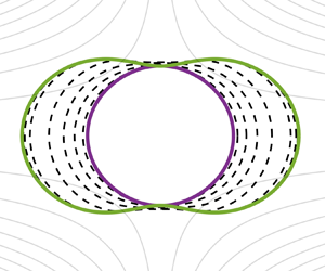
The first test we will perform is a classic shape optimization problem based on (P1). For this problem, we use a high viscosity ratio $\lambda = 48.02$ and capillary number of $\textit {Ca} = 1$, corresponding roughly to a water droplet suspended in air. The far-field boundary conditions for the velocity and pressure are given by

(5.9a,b)\begin{equation} \boldsymbol{u}^\infty = x \boldsymbol{e}_x - \rho \boldsymbol{e}_\rho \quad \text{and} \quad p^\infty = 0. \end{equation}

The initial shape in the optimization is a sphere of radius $R = 1$ and the desired normal velocity field $u_d$ in (3.1) is given by the solution on a geometry from Veerapaneni et al. (Reference Veerapaneni, Gueyffier, Biros and Zorin2009), namely

(5.10)\begin{equation} \left.\begin{array}{c@{}} r(\xi) \triangleq \sqrt{( a \cos^2 (2 {\rm \pi}\, \xi))^2 + (b \sin (2 {\rm \pi}\, \xi))^2)} + \cos^2 (2 {\rm \pi}k\, \xi), \\ \boldsymbol{x}(\xi) \triangleq r(\xi) (\cos(2 {\rm \pi}\, \xi), \sin(2 {\rm \pi}\, \xi)), \end{array}\right\} \end{equation}

with $a = 1, b = 1$ and $k = 1$. The initial geometries and velocity fields are shown in figure 5. The optimization is performed using a standard conjugate gradient descent, as described in algorithm 1 from § 4.8, using the Fletcher–Reeves update formula from Hager & Zhang (Reference Hager and Zhang2006). We choose a regularization parameter of $10^{-2}$ (Eilers Reference Eilers2003) and the smoothing is performed at every step of the optimization. Finally, the discretization continues to follow the parameters described in table 1 with $M = 64$ elements.

Figure 5.

Test 3: (a) geometry and (b) normal velocity. Initial conditions (dashed), desired solution (dotted) and optimal solution ($\bullet$).

The optimal solutions are shown in figure 5. We can see that the algorithm reaches both the desired geometry and the desired normal velocity field. In figure 6 we have the per-iteration values of the normalized cost functional and gradient, defined as

(5.11a,b)\begin{equation} \hat{\mathcal{J}}^{(n)} = \frac{\mathcal{J}^{(n)}}{\mathcal{J}^{(1)}} \quad \text{and} \quad \|\hat{\boldsymbol{g}}^{(n)}\|_\infty = \frac{\|\boldsymbol{g}^{(n)}\|_\infty}{\|\boldsymbol{g}^{(1)}\|_\infty}. \end{equation}

Figure 6.

Test 3: (a) cost functional and (b) descent directions. Absolute values (full) normalized by first iteration (dashed) and Fletcher–Reeves descent direction (dotted).

The optimization algorithm was terminated after $128$ iterations. We can see that the cost functional itself was decreased by approximately six orders of magnitude and plateaus when approaching the optimum. We have found that, with the chosen smoothing, the optimization is sufficiently robust and optimal solutions can be retrieved, with reasonable choices of initial conditions. Of course, this is a highly nonlinear optimization problem, so we do expect the existence of local minima, which a gradient descent algorithm cannot overcome.

5.2.2. Test 4: matching droplet evolution

Next, we look at a quasi-static optimization problem. The physical set-up we will be considering is Taylor's ‘four roller’ apparatus, described and analysed in Taylor (Reference Taylor1934) (see figure 7). The same deformation problem of a droplet in extensional flow was studied in Stone & Leal (Reference Stone and Leal1989). The problem is one of boundary control, where the boundary conditions at ‘infinity’ are given by the (dimensional) velocity field

(5.12)\begin{equation} \boldsymbol{u}^\infty = C (x \boldsymbol{e}_x - \rho \boldsymbol{e}_\rho), \end{equation}

with $C > 0$, the strain rate, as a control parameter. In the non-dimensional equations, this amounts to using the capillary number

(5.13)\begin{equation} \textit{Ca} = \frac{\mu_+ C}{\gamma}, \end{equation}

as a control variable. The viscosity ratio is $\lambda = 48.02$. This is a high viscosity ratio, similar to Taylor's droplet formed from a tar–pitch mixture.

Figure 7.

Test 4: schematic of Taylor's ‘four roller’ apparatus (not to scale).

The optimization is set-up as follows. The initial guess is given by $\textit {Ca}^{(0)} = 0.1$. The desired geometry in (3.1) is obtained by evolving (2.8) with a capillary number $\textit {Ca}_d = 0.05$. This allows achieving $\mathscr {J}_2 \approx 0$. For the optimization, we use the steepest descent choice of the descent direction, since the control parameter is a scalar. The optimization is run until convergence.

Finally, to evolve the interface, we use the third-order strong-stability-preserving Runge–Kutta method described in § 4.5, with an initial condition $\boldsymbol {X}(0)$, a sphere of radius $R = 1$. The simulation is run to a final time $T = 1$ and a time step of ${\rm \Delta} \tau = 10^{-3}$, with a coarse mesh of $M = 16$ elements and the parameters from table 1. We also include the tangential forcing described in Loewenberg & Hinch (Reference Loewenberg and Hinch1996) and a smoothing filter from Eilers (Reference Eilers2003), with a filter strength of $10^{-4}$.

The results of the optimization can be seen in figure 8. As before, we report the cost and gradient normalized by their initial values. We can see that the cost functional converges to machine precision in only $14$ conjugate gradient iterations.

Figure 8.

Test 4: (a) cost functional and (b) gradient. Normalized by first iteration (dashed) and absolute values (full).

5.3. Test 5: propulsion by Marangoni effects

Finally, we present a quasi-static problem where the control is a prescribed variable surface tension. Such a variation in surface tension can be achieved by a varying surfactant concentration, temperature gradients or electric fields. The first two cases have been studied in Muradoglu & Tryggvason (Reference Muradoglu and Tryggvason2008), for example, to which we refer for further details. We will attempt to find an optimal surfactant distribution on the droplet surface to maximize its propulsion in an otherwise quiescent flow. Due to the variable surface tension, the jump in traction becomes (Prosperetti & Tryggvason Reference Prosperetti and Tryggvason2009)

(5.14)\begin{equation} [\![\, \boldsymbol{f} ]\!] _\lambda = \frac{1}{\textit{Ca}_0} (\gamma \kappa \boldsymbol{n} + \nabla_\varSigma \gamma), \end{equation}

where we take a non-dimensional surface tension that is a perturbation of the constant case

(5.15)\begin{equation} \gamma \triangleq 1 + \epsilon \tilde{\gamma}, \end{equation}

for a small $\epsilon$. The control is taken to be $\tilde {\gamma }$ in the cost functional

(5.16)\begin{equation} \mathscr{J}_3(\tilde{\gamma}) = \tfrac{1}{2} |\boldsymbol{x}_c(T) - \boldsymbol{x}_d|^2, \end{equation}

where $\boldsymbol {x}_d$ is a desired centroid and $\boldsymbol {x}_c(t)$ is the centroid at time $t$, as given by

(5.17)\begin{equation} \boldsymbol{x}_c \triangleq \frac{1}{|\varOmega_-|} \int_{\varOmega_-(t)} \boldsymbol{x} \, \textrm{d} V =\frac{1}{|\varOmega_-|} \int_{\varSigma(t)} \frac{1}{2} \|\boldsymbol{x}\|^2 \boldsymbol{n} \, {\rm d} S. \end{equation}

As this is a different optimization problem, we must expand on the results from § 3 to allow for the proposed changes. First, we have that the shape gradient and adjoint-based gradient of the cost functional are

(5.18)\begin{equation} \left.\begin{array}{c@{}} \boldsymbol{\nabla} _{\boldsymbol{X}} \mathcal{J}_3 = \dfrac{1}{|\varOmega_-|} (\boldsymbol{x}_c(T) - \boldsymbol{x}_d) \boldsymbol{\cdot} (\boldsymbol{X}(T) - \boldsymbol{x}_c(T)), \\ \nabla_{\tilde{\gamma}} \mathscr{J}_3 = \dfrac{\epsilon}{\textit{Ca}_0} (2 \kappa \boldsymbol{u}^* \boldsymbol{\cdot} \boldsymbol{n} + (\boldsymbol{n} \boldsymbol{\cdot} \boldsymbol{\nabla} \boldsymbol{u}^*) \boldsymbol{\cdot} \boldsymbol{n}). \end{array}\right\} \end{equation}

To finalize the definitions from lemma 3.7, the source term arising from the jump conditions becomes

(5.19)\begin{equation} \mathcal{C}^*[\boldsymbol{w}^*; \boldsymbol{X}] \triangleq \frac{1}{\textit{Ca}_0} ( \kappa^*[\gamma \boldsymbol{u}^* \boldsymbol{\cdot} \boldsymbol{n}] + n^*[\gamma \kappa \boldsymbol{u}^* \boldsymbol{\cdot} \boldsymbol{t}] + \kappa \boldsymbol{u}^* \boldsymbol{\cdot} \boldsymbol{j} + \langle \boldsymbol{n} \boldsymbol{\cdot} \boldsymbol{\nabla} \boldsymbol{u}^* \rangle \boldsymbol{\cdot} \boldsymbol{j} ), \\ \end{equation}

where $\boldsymbol {j} \triangleq \gamma \kappa \boldsymbol {n} + \nabla _\varSigma \gamma$. An important difference in this case is that the last term now involves an averaging of the normal adjoint velocity gradient, since $\boldsymbol {j}$ also has a tangential component. All the terms can be obtained by following the steps described in appendix C.

For the fluid problem, we choose a quiescent flow $\boldsymbol {u}^\infty = 0$ and $p^\infty = 0$ with an initial condition $\boldsymbol {X}(0)$ given as a sphere of radius $R = 1$. The parameters are given by $\textit {Ca}_0 = 0.05, \lambda = 1$ and $\epsilon = -0.15$. The equations are evolved to a final time of $T = 1$ with a Courant number of $\theta = 0.75$ in (4.15). We have found that the resulting time steps ensure stability for all the configurations found during the optimization.

The optimization is started with an initial guess of

(5.20)\begin{equation} \tilde{\gamma}^{(0)} \triangleq \sin\left(\frac{\rm \pi}{4} \cos (2 \theta) \right), \end{equation}

which is symmetric around $\theta = {\rm \pi}/ 2$, as seen in figure 9(b). Due to this symmetry, the initial guess does not transport the droplet, but simply changes its shape, while remaining centred at $\boldsymbol {x}_c(0) = 0$. The desired centroid is taken to be at a distance of 10 times the radius of the initial sphere, i.e. we have $\boldsymbol {x}_d = (10R, 0)$. For the descent direction, we have used the simpler steepest descent.

Figure 9.

Test 5: (a) cost functional and (b) surface tension along iterations of the optimization algorithm.

The cost functional and the control $\tilde {\gamma }$ during the optimization can be seen in figure 9 and figure 10. As before we can see that the cost correctly converges to the desired centroid location with a final value that approaches machine precision. The optimization was stopped when a step size that satisfied the Armijo condition could not be found, due to the small value of the cost functional. Additional results for a non-symmetric initial distribution of $\tilde {\gamma }$ have shown a clear tendency to evolve the droplets in the direction of larger surface tension, as also shown in Muradoglu & Tryggvason (Reference Muradoglu and Tryggvason2008) for a more general case. This is a well known result for variable surface tension problems.

Figure 10.

Test 5: geometry at the final time $T$ along iterations of the optimization algorithm.