1 Introduction
A capillary bridge may form when a volume of liquid is introduced between adjacent particles. Capillary bridges occur in many applications in science and engineering (such as mechanical strength and ageing of granular materials; gravure printing; colloidal aggregation; solid adhesion; caking; agglomeration; surface cleaning; particle-stabilised foams and emulsions; see for example the references given by Bostwick & Steen (Reference Bostwick and Steen2015) and by Lian & Seville (Reference Lian and Seville2016)).
The properties of steady capillary bridges between two spheres of identical radius have therefore been studied extensively, especially in the pendular regime where a single capillary bridge exists between two spheres. Of particular interest is the dependence of the capillary force on the volume of the capillary bridge and on the separation between the spheres. Corresponding experiments have been performed by Mason & Clark (Reference Mason and Clark1965), Willett et al. (Reference Willett, Adams, Johnson and Seville2000) and Rabinovich, Esayanur & Moudgil (Reference Rabinovich, Esayanur and Moudgil2005).
The geometry of a steady capillary bridge surface is described by the Young–Laplace equation, according to which the mean curvature of this surface is constant in the absence of gravity. Solutions of the Young–Laplace equation for axisymmetric capillary bridges have been reported in the literature (for example Erle, Dyson & Morrow Reference Erle, Dyson and Morrow1971; Orr, Scriven & Rivas Reference Orr, Scriven and Rivas1975; Kralchevsky & Nagayama Reference Kralchevsky and Nagayama2001) for nodoid, catenoid and unduloid cases. These solutions for the meridional profile of the capillary bridge surface are formulated in terms of elliptical functions.
Approximations have been developed to simplify these expressions and to gain additional understanding of the important parameters. An often employed approximation is the toroidal approximation (see for example Fisher Reference Fisher1926; Orr et al. Reference Orr, Scriven and Rivas1975; Lian, Thornton & Adams Reference Lian, Thornton and Adams1993; Rabinovich et al. Reference Rabinovich, Esayanur and Moudgil2005; Megias-Alguacil & Gauckler Reference Megias-Alguacil and Gauckler2011; Harireche, Faramarzi & Alani Reference Harireche, Faramarzi and Alani2013, Reference Harireche, Faramarzi and Alani2015; Ardito et al. Reference Ardito, Corigliano, Frangi and Rizzini2014) in which the meridional profile of the capillary bridge is described by an arc (part of a circle). This toroidal approximation leads to a varying mean curvature of the capillary bridge surface, which is inconsistent with the governing Young–Laplace equation. The accuracy of the toroidal approximation has been investigated in various studies, such as by Orr et al. (Reference Orr, Scriven and Rivas1975), Megias-Alguacil & Gauckler (Reference Megias-Alguacil and Gauckler2011) and especially by Lian et al. (Reference Lian, Thornton and Adams1993), who also compared various ways of evaluating the capillary force with the toroidal approximation. In the (simplified) Derjaguin approximation (see for example Israelachvili Reference Israelachvili2011; Lian & Seville Reference Lian and Seville2016) the meridional curvature is neglected in the evaluation of the capillary force.
Based on numerical solutions of the Young–Laplace equation, Erle et al. (Reference Erle, Dyson and Morrow1971) have shown that, for an identical volume of the capillary bridge and the separation between the spheres, two solutions for the meridional profile may exist. The separation at which the two branches for the solution coincide corresponds to the rupture distance, i.e. the maximum separation
 $S_{crit}$
between the spheres.
Lian et al. (Reference Lian, Thornton and Adams1993) have formulated a rupture criterion for this critical separation. Their criterion is based on many numerical solutions of the Young–Laplace equation. According to their criterion, the critical separation
 $S_{crit}$
is determined by the volume
 $V$
of the capillary bridge:
 $$\begin{eqnarray}\displaystyle S_{crit}=0.5V^{1/3} & & \displaystyle\end{eqnarray}$$
for the case of zero wetting angle. Willett et al. (Reference Willett, Adams, Johnson and Seville2000) have extended the rupture criterion of Lian et al. (Reference Lian, Thornton and Adams1993) by accounting for larger capillary bridge volumes and for differences in radius of the two spheres. The criterion, (1.1), for the critical separation is in good agreement with results of measurements by Mason & Clark (Reference Mason and Clark1965) and Willett et al. (Reference Willett, Adams, Johnson and Seville2000).
In simulations using the Discrete Element Method (as developed by Cundall & Strack Reference Cundall and Strack1979) of the cohesive behaviour of granular systems (see for example Soulié et al. Reference Soulié, Cherblanc, El Youssoufi and Saix2006; Richefeu, El Youssoufi & Peyroux Reference Richefeu, El Youssoufi, Peyroux and Radjaï2008; Than et al. Reference Than, Khamseh, Tang, Pereira, Chevoir and Roux2016) expressions for the capillary force as a function of the volume of the capillary bridge and the particle separation are required. Such expressions are often based on fits to data from numerical solutions of the Young–Laplace equation (for example Willett et al. Reference Willett, Adams, Johnson and Seville2000; Soulié et al. Reference Soulié, Cherblanc, El Youssoufi and Saix2006; Richefeu et al. Reference Richefeu, El Youssoufi, Peyroux and Radjaï2008; Lian & Seville Reference Lian and Seville2016). Gladkyy & Schwarze (Reference Gladkyy and Schwarze2014) have compared the predictions for the capillary force as a function of the capillary bridge volume and the particle separation according to several relations from the literature with experimental results by Willett et al. (Reference Willett, Adams, Johnson and Seville2000) and by Rabinovich et al. (Reference Rabinovich, Esayanur and Moudgil2005). They also showed that the influence on the macroscopic behaviour of the employed relation for the capillary force in simulations of granular systems using the Discrete Element Method is rather small.
Previous studies of the capillary force and of the critical separation have been based either on numerical solutions of the Young–Laplace equation or on a simplified analytical description of the capillary bridge geometry in the toroidal approximation. The current analytical study complements previous numerical and analytical studies by proposing an improved geometrical description of the capillary bridge that reflects properties of the Young–Laplace equation. Specific objectives of the current study are to:
-
(i) show analytically that two (approximate) solutions of the Young–Laplace equation exist (for an identical capillary bridge volume and particle separation smaller than the critical separation), as Erle et al. (Reference Erle, Dyson and Morrow1971) noted from their numerical solutions;
-
(ii) develop in an analytical manner a rupture criterion by showing that, beyond a critical separation, no solution exists for the meridional profile;
-
(iii) formulate closed-form relations for the capillary force, as a function of the capillary bridge volume and the separation between the spheres, that are based on analytical considerations.
The current study is restricted to steady, axisymmetric capillary bridges between rigid spheres. Some studies focusing on cases where these assumptions do not hold are the following. Farmer & Bird (Reference Farmer and Bird2015) have shown experimentally and computationally that capillary bridges between spheres in contact may become non-axisymmetric at large capillary bridge volumes. Wexler, Heard & Stone (Reference Wexler, Heard and Stone2014) have studied experimentally and theoretically capillary bridges between soft elastic bodies. Capillary bridges between a plane and a cylinder have been studied experimentally and theoretically by Reyssat (Reference Reyssat2015). The rupture of a capillary bridge is a transient process, see for example Eggers & Villermaux (Reference Eggers and Villermaux2008) and Li & Sprittles (Reference Li and Sprittles2016). The stability of capillary bridges is not addressed here, see the recent overview by Bostwick & Steen (Reference Bostwick and Steen2015) on the stability of capillary surfaces. Instabilities during evaporation of a capillary bridge have been studied experimentally by Mielniczuk, Hueckel & Youssoufi (Reference Mielniczuk, Hueckel and El Youssoufi2015).
The outline of this study is as follows. The geometry of the capillary bridge in the considered pendular regime is described in § 2. The Young–Laplace equation, some of its properties and the adopted approach for its numerical resolution are given in § 3. Numerical solutions of the Young–Laplace equations are used here to assess the accuracy of the developed approximate analytical theory. The analytical theory is formulated in § 4, where results for the capillary forces are also given. Finally, the findings from this study are discussed in § 5.
2 Geometry of the capillary bridge in the pendular regime
The focus here is on axisymmetric capillary bridges between two particles in the pendular regime. These particles are considered to be two spheres with identical radius
 $a$
. All meridional coordinates, which describe the geometry of the liquid–gas interface of the capillary bridge, are made non-dimensional with respect to the radius
 $a$
. These non-dimensional coordinates are denoted by
 $X$
and
 $Y$
. The meridional profile of the surface of the capillary bridge is denoted by
 $Y(X)$
, which gives the local radius of the axisymmetric capillary bridge at axial coordinate
 $X$
. The separation between the spheres is
 $2aS$
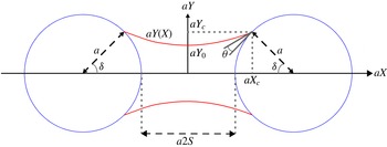
. The meridional coordinates of the three-phase contact circle at the sphere on the right are
 $(X_{c},Y_{c})$
. The meridional coordinates at the neck (or ‘gorge’) are
 $(0,Y_{0})$
. These geometrical quantities are illustrated in figure 1. Coordinate
 $Y_{0}$
is called the neck radius and
 $Y_{c}$
the contact radius (an abbreviation for radius of the three-phase contact circle at the sphere).
Meridional geometry of an axisymmetric capillary bridge between two equal-sized spheres with radius
 $a$
.

The meridional coordinates of the contact circle
 $(X_{c},Y_{c})$
at the sphere are related to the (half) filling angle
 $\unicode[STIX]{x1D6FF}$
(see also figure 1) and the (half) separation
 $S$
by
 $$\begin{eqnarray}\displaystyle X_{c}=S+1-\cos \unicode[STIX]{x1D6FF},\quad Y_{c}=\sin \unicode[STIX]{x1D6FF}. & & \displaystyle\end{eqnarray}$$
To enable analytical developments, the analyses presented here are restricted to small filling angles
 $\unicode[STIX]{x1D6FF}$
, and hence small contact radii
 $Y_{c}$
. Then it follows by a Taylor expansion in
 $\unicode[STIX]{x1D6FF}$
(around zero) from (2.1) that
 $$\begin{eqnarray}\displaystyle X_{c}\cong S+{\textstyle \frac{1}{2}}Y_{c}^{2},\quad Y_{c}\cong \unicode[STIX]{x1D6FF}. & & \displaystyle\end{eqnarray}$$
3 Young–Laplace equation
The meridional profile
 $Y(X)$
of an axisymmetric capillary bridge is described by the Young–Laplace equation, according to which the mean curvature of the liquid–gas interface is constant in the absence of gravity. The Young–Laplace equation is given here in non-dimensional form,
 $$\begin{eqnarray}\displaystyle K[Y]=H, & & \displaystyle\end{eqnarray}$$
where
 $K[Y]$
is the curvature operator that gives the local (i.e. at position
 $X$
) mean curvature of the axisymmetric capillary bridge surface corresponding to the meridional profile
 $Y(X)$
(see for example Orr et al.
Reference Orr, Scriven and Rivas1975; Lian et al.
Reference Lian, Thornton and Adams1993; Kralchevsky & Nagayama Reference Kralchevsky and Nagayama2001):
 $$\begin{eqnarray}\displaystyle K[Y]\equiv \frac{1}{Y}\frac{1}{(1+Y^{\prime 2})^{1/2}}-\frac{Y^{\prime \prime }}{(1+Y^{\prime 2})^{3/2}}. & & \displaystyle\end{eqnarray}$$
Here
 $Y^{\prime }=\text{d}Y/\text{d}X$
and
 $Y^{\prime \prime }=\text{d}^{2}Y/\text{d}X^{2}$
. The constant mean curvature
 $H$
in (3.1) is given by
 $$\begin{eqnarray}\displaystyle H=a\frac{p_{int}-p_{ext}}{\unicode[STIX]{x1D6FE}}, & & \displaystyle\end{eqnarray}$$
where
 $\unicode[STIX]{x1D6FE}$
is the surface tension (
 $\unicode[STIX]{x1D6FE}=72.8\times 10^{-3}~\text{N}~\text{m}^{-1}$
for water–air interfaces at a temperature of
 $20\,^{\circ }\text{C}$
) and
 $p_{int}-p_{ext}$
is the capillary pressure difference across the liquid–gas interface (
 $p_{ext}$
and
 $p_{int}$
are the pressures exterior (gas) and interior (liquid) to the capillary bridge, respectively).
Boundary conditions at the contact circle (at
 $X=X_{c}$
) for the second-order nonlinear ordinary differential equation (3.1) are
 $$\begin{eqnarray}\displaystyle Y(X_{c})=\sin \unicode[STIX]{x1D6FF}\equiv Y_{c},\quad Y^{\prime }(X_{c})=\cot (\unicode[STIX]{x1D6FF}+\unicode[STIX]{x1D703})\equiv Y_{c}^{\prime }, & & \displaystyle\end{eqnarray}$$
where
 $\unicode[STIX]{x1D703}$
is the wetting angle (also indicated in figure 1). At the neck,
 $X=0$
, boundary conditions are
 $$\begin{eqnarray}\displaystyle Y(0)=Y_{0},\quad Y^{\prime }(0)=0, & & \displaystyle\end{eqnarray}$$
where the latter condition is due to the symmetry of the capillary bridge between the two identical spheres. In the present study, only the case of perfectly wettable spheres, with wetting angle
 $\unicode[STIX]{x1D703}=0^{\circ }$
, is considered.
Solutions to the Young–Laplace equation (3.1) have a first integral (see for example Erle et al. Reference Erle, Dyson and Morrow1971; Lian et al. Reference Lian, Thornton and Adams1993; Gagneux & Millet Reference Gagneux and Millet2014)
 $$\begin{eqnarray}\displaystyle \frac{Y}{\sqrt{1+Y^{\prime 2}}}+\frac{1}{2}HY^{2}=\text{const.}=\unicode[STIX]{x1D706}. & & \displaystyle\end{eqnarray}$$
Equation (3.6) also results from force equilibrium considerations of an axially infinitesimal cross-section of the capillary bridge, where forces due to internal pressure, external pressure and surface tension are accounted for.
It follows from (3.6) that the parameters
 $H$
and
 $\unicode[STIX]{x1D706}$
can be expressed in terms of the neck radius
 $Y_{0}$
, the contact radius
 $Y_{c}$
and the meridional slope at the contact circle
 $Y_{c}^{\prime }$
(defined in (3.4)) by
 $$\begin{eqnarray}\displaystyle \frac{1}{2}H=\frac{Y_{0}-\displaystyle \frac{Y_{c}}{\sqrt{1+Y_{c}^{\prime 2}}}}{Y_{c}^{2}-Y_{0}^{2}},\quad \unicode[STIX]{x1D706}=Y_{0}+\frac{1}{2}HY_{0}^{2}, & & \displaystyle\end{eqnarray}$$
where (3.5) has been used.
For the case of zero wetting angle,
 $\unicode[STIX]{x1D703}=0^{\circ }$
, and small values of the contact radius
 $Y_{c}$
, it follows by Taylor expansion in
 $\unicode[STIX]{x1D6FF}$
(around zero) that the second boundary condition in (3.4) can be approximated by
 $$\begin{eqnarray}\displaystyle Y^{\prime }(X_{c})=Y_{c}^{\prime }\cong \frac{1}{Y_{c}}, & & \displaystyle\end{eqnarray}$$
where (2.2) has been used. Then the expression for the constant mean curvature
 $H$
in (3.7) can be approximated by (as the neck radius
 $Y_{0}$
is also small)
 $$\begin{eqnarray}\displaystyle \frac{1}{2}H\cong \frac{Y_{c}}{Y_{c}^{2}-Y_{0}^{2}}-1. & & \displaystyle\end{eqnarray}$$
The (dimensionless) constant
 $\unicode[STIX]{x1D706}$
in (3.7) is related to the (dimensional) capillary force
 $F_{cap}$
by
 $$\begin{eqnarray}\displaystyle \frac{F_{cap}}{2\unicode[STIX]{x03C0}a\unicode[STIX]{x1D6FE}}=\unicode[STIX]{x1D706}. & & \displaystyle\end{eqnarray}$$
A positive value for the capillary force
 $F_{cap}$
corresponds to a tensile force between the two spheres.
Willett et al. (Reference Willett, Adams, Johnson and Seville2000) showed that the capillary forces, as determined from the numerical solution of the Young–Laplace equation, agree well with the capillary forces as measured in their comprehensive experiments for a range of interparticle separations and capillary bridge volumes.
3.1 Numerical resolution of the Young–Laplace equation
Numerical solutions to the Young–Laplace equation (3.1) have been obtained here in the following manner for the right part (
 $X\geqslant 0$
) of the symmetrical (around
 $X=0$
) capillary bridge profile
 $Y(X)$
. With fixed neck radius
 $Y_{0}$
and contact radius
 $Y_{c}$
(
 $Y_{c}^{\prime }$
is determined by
 $Y_{c}$
through (3.8)), parameters
 $H$
and
 $\unicode[STIX]{x1D706}$
can be determined from (3.7). From (3.6),
 $\text{d}Y/\text{d}X$
can then be expressed as a function of
 $Y$
. Then the meridional profile
 $X(Y)$
, the dual of
 $Y(X)$
with
 $\text{d}X/\text{d}Y=1/(\text{d}Y/\text{d}X)$
, is obtained directly from the integral
 $$\begin{eqnarray}\displaystyle X_{c}-X(Y)=\int _{Y}^{Y_{c}}\frac{\left(\unicode[STIX]{x1D706}-\displaystyle \frac{1}{2}HY^{2}\right)}{\sqrt{Y^{2}-\left(\unicode[STIX]{x1D706}-\displaystyle \frac{1}{2}HY^{2}\right)^{2}}}\,\text{d}Y. & & \displaystyle\end{eqnarray}$$
The integral in (3.11) is evaluated numerically using an adaptive step-size (with respect to the specified relative error tolerance of
 $10^{-6}$
) Gauss–Kronrod quadrature. In the present formulation the integrand in (3.11) contains a weak (square-root) singularity at
 $Y_{0}$
. The integration method has been tested separately for a problem to which an analytical solution is available in order to verify that the employed integration method captures the solution with sufficient accuracy for such singularities. For the case given by Erle et al. (Reference Erle, Dyson and Morrow1971) in their figure 5, the current results agreed with theirs up to the reported number of digits. Example solutions for the meridional profile
 $Y(X)$
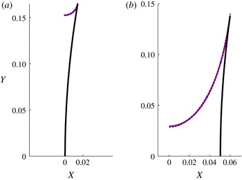
for small and for large separations are shown in figure 2. Also shown in figure 2 are elliptical fits to the meridional profile
 $Y(X)$
that are discussed in § 4.1.
Meridional profiles
 $Y(X)$
of the capillary bridge obtained by numerically solving the Young–Laplace equation (red, solid lines) and elliptical fits (blue, dotted lines). The symmetrical meridional profile is only shown for
 $X\geqslant 0$
. Part of the right sphere is shown in black. (a) Small separation
 $S$
(parameters:
 $Y_{c}=0.1648$
,
 $Y_{0}=0.1524$
). (b) Large separation
 $S$
(parameters:
 $Y_{c}=0.1385$
,
 $Y_{0}=0.0295$
). Aspect ratios of fitted ellipses: (a) 0.98; (b) 0.41.

Erle et al. (Reference Erle, Dyson and Morrow1971) solved the Young–Laplace equation as an ordinary differential equation for the meridional profile
 $Y(X)$
, starting their computation at the contact circle and ending when the slope of the meridional profile becomes zero. Lian et al. (Reference Lian, Thornton and Adams1993) also solved the Young–Laplace equation as an ordinary differential equation for
 $Y(X)$
, but starting at the neck and ending when an intersection is found with the sphere. The current approach is (slightly) simpler as only an integral (rather than an ordinary differential equation) has to be evaluated. The adopted numerical quadrature is well suited to resolve the weak singularity at the neck.
In the adopted approach where the neck and contact radii,
 $Y_{0}$
and
 $Y_{c}$
respectively, are fixed and used to compute
 $H$
and
 $\unicode[STIX]{x1D706}$
, the separation
 $S$
is a (unique) result of the computation.
The dimensionless volume
 $V$
(i.e. scaled by
 $a^{3}$
) and the dimensionless area
 $A$
(i.e. scaled by
 $a^{2}$
) of the capillary bridge (both also including the part corresponding to
 $X\leqslant 0$
) are subsequently obtained from the meridional profile
 $Y(X)$
by integration:
 $$\begin{eqnarray}\displaystyle V=2\unicode[STIX]{x03C0}\int _{0}^{X_{c}}Y^{2}\,\text{d}X-2V_{cap},\quad A=4\unicode[STIX]{x03C0}\int _{0}^{X_{c}}Y\sqrt{1+Y^{^{\prime }2}}\,\text{d}X, & & \displaystyle\end{eqnarray}$$
where
 $V_{cap}=\unicode[STIX]{x03C0}/3(1-\cos \unicode[STIX]{x1D6FF})^{2}(2+\cos \unicode[STIX]{x1D6FF})$
is the volume of the cap (i.e. the part of the sphere up to
 $X=X_{c}$
; see also Gagneux & Millet Reference Gagneux and Millet2014). The integrals in (3.12) have been evaluated numerically, based on 500 points at which the meridional profile
 $Y(X)$
has been stored, to determine the volume
 $V$
and the area
 $A$
of the capillary bridge from the numerical solution of the Young–Laplace equation.
A large number of numerical solutions to the Young–Laplace equation has been computed, for filling angles
 $\unicode[STIX]{x1D6FF}\leqslant 30^{\circ }$
(1000 different values have been considered) and ratios
 $0<Y_{0}/Y_{c}<1$
(again 1000 different values have been considered). For
 $0<Y_{0}/Y_{c}<1$
, concave capillary bridge profiles are obtained. Non-physical solutions with separation
 $S<0$
(recalling that the separation
 $S$
between the spheres is a result of the computation with
 $Y_{0}$
and
 $Y_{c}$
prescribed) have been disregarded.
For sets of specified values for the filling angle
 $\unicode[STIX]{x1D6FF}$
(equivalent to
 $Y_{c}$
) and for the ratio
 $Y_{0}/Y_{c}$
, sets of values for the separation
 $S$
, the capillary bridge volume
 $V$
and other parameters of interest, such as the capillary force
 $F_{cap}$
, are obtained from the numerical solution of the Young–Laplace equation. Based on (sub)sets of values
 $\{V_{i},S_{i}\}$
, the Delaunay triangulation can be determined. Using this triangulation and values such as
 $\{F_{cap,i}\}$
, values for capillary bridge properties such as
 $F_{cap}$
can be computed by linear interpolation at an arbitrary point
 $(V,S)$
within the convex hull corresponding to the set of values
 $\{V_{i},S_{i}\}$
.
4 Analytical theory
The numerical solutions of the Young–Laplace equation depicted in figure 2 demonstrate that, in general, the meridional profile
 $Y(X)$
cannot be described accurately by an arc (part of a circle) as is assumed in the toroidal approximation. The current approach forms a generalisation of the toroidal approximation, because the description of the meridional profile
 $Y(X)$
is based on a part of an ellipse. Geometrical aspects of this elliptical profile are described in § 4.1. Since this description of the meridional profile
 $Y(X)$
by a part of an ellipse contains an additional, free geometrical parameter, in comparison to the description by an arc, a supplementary relation is required. This ‘closure’ relation is given in § 4.2. Aspects of the determination of the contact radius
 $Y_{c}$
from the volume
 $V$
of the capillary bridge and the separation
 $S$
are described in § 4.3. The rupture criterion for the critical separation
 $S_{crit}$
, which is the direct result of the current analytical approach, is formulated in § 4.4. Finally, an expression for the capillary force, as a function of the volume
 $V$
of the capillary bridge and the separation
 $S$
between the spheres, is given in § 4.5.
4.1 Elliptical capillary bridge profile
In the toroidal approximation (see for example Fisher Reference Fisher1926; Lian et al.
Reference Lian, Thornton and Adams1993) the meridional profile
 $Y(X)$
of the capillary bridge surface is described by an arc (part of a circle), with parameters that are completely determined by the boundary conditions, (3.4) and (3.5) at the contact circle and at the neck.
In the current analytical description the meridional profile
 $Y(X)$
is described by part of the bottom half of an ellipse with centre at
 $(0,M)$
and lengths of half-axes
 $B$
and
 $C$
:
 $$\begin{eqnarray}\displaystyle \frac{X^{2}}{B^{2}}+\frac{(M-Y)^{2}}{C^{2}}=1. & & \displaystyle\end{eqnarray}$$
This elliptical representation involves an additional, free parameter in comparison to the toroidal approximation where
 $B=C$
.
Some meridional profiles
 $Y(X)$
of the capillary bridge, which have been obtained through the numerical solution of the Young–Laplace equation, are shown in figure 2 in combination with corresponding elliptical fits to illustrate the accuracy of the description of the meridional profile by a part of an ellipse. The elliptical fits are virtually indistinguishable from the (effectively exact) numerical solutions. For the case with large separation shown in figure 2(b) it is clear that the meridional profile cannot, in general, be described accurately by an arc as is done in the toroidal approximation. Other fits, such as polynomial fits, resulted in significantly larger discrepancies with numerical solutions, in comparison to the description of the meridional profile
 $Y(X)$
by a part of an ellipse.
The three parameters
 $M$
,
 $B$
and
 $C$
in the elliptical representation, equation (4.1), can be related to the meridional coordinates at the contact circle
 $X_{c}$
,
 $Y_{c}$
, the neck radius
 $Y_{0}$
and the slope at the contact circle
 $Y_{c}^{\prime }$
through the requirements
 $$\begin{eqnarray}\displaystyle Y(X_{c})=Y_{c},\quad Y^{\prime }(X_{c})=Y_{c}^{\prime },\quad Y(0)=Y_{0}, & & \displaystyle\end{eqnarray}$$
where
 $Y_{c}^{\prime }$
is given in (3.4), and in approximate form in (3.8) for the case considered here with wetting angle
 $\unicode[STIX]{x1D703}=0^{\circ }$
. Note that the elliptical meridional profile, (4.1), automatically satisfies the symmetry condition
 $Y^{\prime }(0)=0$
in (3.5). After some algebra it follows that these parameters are given by
 $$\begin{eqnarray}\displaystyle M=\frac{Y_{c}X_{c}Y_{c}^{\prime }-(Y_{c}^{2}-Y_{0}^{2})}{X_{c}Y_{c}^{\prime }-2(Y_{c}-Y_{0})},\quad C=M-Y_{0},\quad B=\frac{X_{c}}{\sqrt{1-\displaystyle \left(\frac{M-Y_{c}}{M-Y_{0}}\right)^{2}}}.\quad & & \displaystyle\end{eqnarray}$$
Coordinates
 $X_{c}$
and
 $Y_{0}$
will vary with
 $Y_{c}$
. Therefore, the following scaling is introduced:
 $$\begin{eqnarray}\displaystyle P=\frac{X_{c}}{Y_{c}},\quad Q=\frac{Y_{0}}{Y_{c}}. & & \displaystyle\end{eqnarray}$$
Thus,
 $P$
represents the scaled axial position of the contact circle and
 $Q$
represents the scaled neck radius.
For small values of the contact radius
 $Y_{c}$
it follows (after some algebra) from (3.8), (4.3) and (4.4) by Taylor expansion in
 $Y_{c}$
that the ellipse parameters
 $M$
,
 $B$
and
 $C$
can be approximated by
 $$\begin{eqnarray}\displaystyle M\cong Y_{c}+\frac{(1-Q)^{2}}{P}Y_{c}^{2},\quad C\cong (1-Q)Y_{c}+\frac{(1-Q)^{2}}{P}Y_{c}^{2},\quad B\cong PY_{c}+\frac{(1-Q)^{2}}{2P}Y_{c}^{3}. & & \displaystyle \nonumber\\ \displaystyle & & \displaystyle\end{eqnarray}$$
Note that in the toroidal approximation
 $B=C$
, and hence
 $P\cong 1-Q$
for small values of the contact radius
 $Y_{c}$
.
4.2 ‘Closure’ relation
The assumed elliptical shape of the meridional profile
 $Y(X)$
contains the parameters
 $Y_{c}$
,
 $X_{c}$
(or
 $P$
) and
 $Y_{0}$
(or
 $Q$
). With prescribed contact radius
 $Y_{c}$
and separation
 $S$
, the neck radius
 $Y_{0}$
is a free parameter whose value has to be determined from an additional ‘closure’ relation.
The toroidal approximation does not account for properties of the Young–Laplace equation, according to which the mean curvature of the capillary bridge surface is constant. Therefore, in the toroidal approximation the capillary force can be evaluated in different ways (either at the neck or at the contact circle) that differ in their agreement with the capillary force obtained from the numerical solution of the Young–Laplace equation (Lian et al. Reference Lian, Thornton and Adams1993).
The additional closure relation is obtained here by requiring that the mean curvature at the neck,
 $X=0$
, be equal to the mean curvature at the contact circle,
 $X=X_{c}$
:
 $$\begin{eqnarray}\displaystyle K[Y](X=0)=K[Y](X=X_{c}). & & \displaystyle\end{eqnarray}$$
The mean curvature
 $K[Y]$
, defined in (3.2), corresponding to the meridional profile
 $Y(X)$
can be evaluated from the adopted elliptical description of the meridional profile
 $Y(X)$
, (4.1). After substitution of the parameters
 $M$
,
 $B$
and
 $C$
from (4.5) into (4.6), it follows (after some algebra that has been performed with the symbolic mathematics package Maple) that, up to leading order in the contact radius
 $Y_{c}$
, the additional closure relation (4.6) can be expressed as a relationship between the parameters
 $P$
and
 $Q$
(as defined in (4.4)):
 $$\begin{eqnarray}\displaystyle h(P)\equiv QP^{3}+(1-Q)^{2}P^{2}-Q(1-Q)^{3}=0. & & \displaystyle\end{eqnarray}$$
As
 $h(0)\leqslant 0$
and
 $\text{d}h(P)/\text{d}P\geqslant 0$
for
 $0\leqslant Q\leqslant 1$
and
 $P\geqslant 0$
, it follows that the cubic equation (4.7) for
 $P$
(given
 $Q$
) has a single real, non-negative root. Therefore, the solution of the cubic equation (4.7) with
 $P\geqslant 0$
can be expressed as a functional relationship
 $P=F(Q)$
(for
 $0\leqslant Q\leqslant 1$
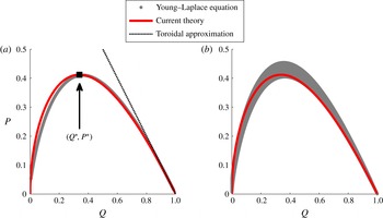
). This function is shown in figure 3(a; red solid line). It is readily verified that for
 $Q\cong 1$
the solution
 $P$
of (4.7) is given by
 $P\cong 1-Q$
, which corresponds to the toroidal approximation. The maximum for
 $P$
, denoted by
 $P^{\ast }$
, is
 $P^{\ast }\cong 0.412$
, which is obtained for
 $Q=Q^{\ast }\cong 0.338$
.
(a) Theoretical closure relation
 $P=F(Q)$
(red, solid line), conforming to the real, non-negative solution of (4.7) for
 $P$
(given
 $Q$
). The ‘critical’ point
 $(Q^{\ast },P^{\ast })$
is indicated that corresponds to the maximum of
 $P=F(Q)$
. Data shown as overlapping grey points correspond to numerical solutions of the Young–Laplace equation with
 $V\cong 10^{-6}$
and
 $Y_{c}<0.05$
. Also indicated (black, dashed line) is the relation according to the toroidal approximation,
 $P=1-Q$
. (b) Theoretical relation
 $P=F(Q)$
(red, solid line). Data shown as grey points correspond to numerical solutions of the Young–Laplace equation with
 $V<0.05$
and
 $Y_{c}<0.10$
.

For fixed values of the contact radius
 $Y_{c}$
(representative of a fixed capillary bridge volume
 $V$
) and of
 $P$
(representative of a fixed separation
 $S$
; with
 $P\leqslant P^{\ast }$
), two values are possible for
 $Q$
, and hence two solutions exist for the neck radius
 $Y_{0}$
. Erle et al. (Reference Erle, Dyson and Morrow1971) already showed the existence of two solutions, but based on numerical solutions of the Young–Laplace equation.
Results for
 $P$
and
 $Q$
from many numerical solutions of the Young–Laplace equation are shown in figure 3 (a; grey markers, which overlap to form a single grey area) for a capillary bridge volume
 $V\cong 10^{-6}$
and for
 $Y_{c}<0.05$
. The numerical results show the same qualitative behaviour: an increase in
 $P$
with increasing
 $Q$
, up to a critical point, after which
 $P$
decreases. Quantitatively, the numerical results are well described by the theoretical closure relation, (4.7), especially for
 $Q\geqslant Q^{\ast }$
.
Results for a wider range of values for the capillary bridge volume
 $V$
and for the contact radius
 $Y_{c}$
,
 $V<0.05$
and
 $Y_{c}<0.10$
, are shown in figure 3 (b; grey markers). At a fixed value of
 $Q$
, the numerical solutions exhibit a range of values for
 $P$
. There is no longer a (nearly) unique relation between
 $P$
and
 $Q$
, but the numerical results lie in a band around the theoretical curve corresponding to (4.7) (red, solid line). The width of this band is small for small
 $P$
. Note that the theoretical relation (4.7) is valid for small values for the contact radius
 $Y_{c}$
, while the numerical results also involve large values for
 $Y_{c}$
.
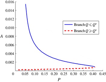
The variation with
 $P$
of the surface area
 $A$
of the capillary bridge (defined in (3.12)), as determined from the numerical solution of the Young–Laplace equation, is shown in figure 4 for the two branches (
 $Q\leqslant Q^{\ast }$
and
 $Q\geqslant Q^{\ast }$
) for cases with
 $V\cong 10^{-6}$
and
 $Y_{c}<0.05$
. Of a pair of such solutions, the solution with the smaller value for
 $Q$
(corresponding to a smaller neck radius
 $Y_{0}$
) will have a larger surface area
 $A$
than the solution with the larger value for
 $Q$
(corresponding to a larger neck radius
 $Y_{0}$
). Only the latter is expected to occur, because it will have a lower surface energy. Thus, only solutions with
 $Q\geqslant Q^{\ast }$
are considered to be physically relevant (see also Erle et al.
Reference Erle, Dyson and Morrow1971; Lian et al.
Reference Lian, Thornton and Adams1993).
Surface area
 $A$
of the capillary bridge as a function of
 $P$
. Data shown correspond to numerical solutions of the Young–Laplace equation with
 $V\cong 10^{-6}$
and
 $Y_{c}<0.05$
. The branch with
 $Q\leqslant Q^{\ast }$
is indicated by a blue solid line, while the branch with
 $Q\geqslant Q^{\ast }$
is indicated by a red dashed line.

Although (complicated) analytical expressions are known for solutions to cubic equations (see for example Korn & Korn Reference Korn and Korn1968), such as (4.7), for the current purposes a simpler approximation is desirable and sufficient. A Padé approximant of the relationship
 $P=F(Q)$
that is convenient for the determination of the two branches of the inverse relation,
 $Q=F^{-1}(P)$
, is described in appendix A.
4.3 Relation between contact radius, capillary bridge volume and separation
The volume
 $V$
of the capillary bridge is given by (3.12). Using the elliptical description for the meridional profile
 $Y(X)$
in (4.1) with the ellipse parameters
 $M$
,
 $B$
,
 $C$
given by (4.5) and taking into account that the contact radius
 $Y_{c}$
is small, the volume
 $V$
of the capillary bridge can be approximated by
 $$\begin{eqnarray}\displaystyle V\cong \frac{\unicode[STIX]{x03C0}}{3}G(Q)PY_{c}^{3}-\frac{\unicode[STIX]{x03C0}}{2}Y_{c}^{4},\quad G(Q)=4Q^{2}+(3\unicode[STIX]{x03C0}-8)Q+(10-3\unicode[STIX]{x03C0}). & & \displaystyle\end{eqnarray}$$
For the two branches,
 $Q\leqslant Q^{\ast }$
and
 $Q\geqslant Q^{\ast }$
, the closure relation for
 $P=F(Q)$
(corresponding to (4.7)) can be inverted. As
 $P$
is defined in (4.4) (with
 $X_{c}$
given in (2.2)) in terms of the contact radius
 $Y_{c}$
and the separation
 $S$
, there are two branches for (4.8) as an equation for
 $Y_{c}$
given the capillary bridge volume
 $V$
and the separation
 $S$
. Thus, it is expected that at identical capillary bridge volume
 $V$
and separation
 $S$
, two (real, positive) solutions for the contact radius
 $Y_{c}$
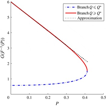
may be obtained. This was shown by Erle et al. (Reference Erle, Dyson and Morrow1971) based on numerical solutions of the Young–Laplace equation. Here this finding has been obtained in an analytical manner.
Two branches of the composite function
 $G(F^{-1}(P))$
, together with the approximation of the branch
 $Q\geqslant Q^{\ast }$
by (4.9).

The two branches for the composite function
 $G(F^{-1}(P))$
are shown in figure 5. As discussed in § 4.2, the solution for the meridional profile for the branch with
 $Q\geqslant Q^{\ast }$
has a smaller surface area
 $A$
of the capillary bridge than the solution for the branch with
 $Q\leqslant Q^{\ast }$
. Therefore, solutions corresponding to the former branch
 $Q\geqslant Q^{\ast }$
are considered to be relevant here. As indicated in figure 5, the branch corresponding to
 $Q\geqslant Q^{\ast }$
can be well approximated by
 $$\begin{eqnarray}\displaystyle G(F^{-1}(P))\cong 6-3\unicode[STIX]{x03C0}P. & & \displaystyle\end{eqnarray}$$
This approximation is based on a first-order Taylor expansion of
 $G(F^{-1}(P))$
around
 $P=0$
,
 $Q=1$
. This approximation is accurate for
 $P\leqslant 0.35$
.
Combining the approximation (4.9) with the expression (4.8) for the capillary bridge volume
 $V$
and using (2.2) and (4.4) to express
 $P$
in terms of
 $S$
and
 $Y_{c}$
yields a quintic equation in the contact radius
 $Y_{c}$
(given the capillary bridge volume
 $V$
and the separation
 $S$
):
 $$\begin{eqnarray}\displaystyle \left(\frac{-\unicode[STIX]{x03C0}}{2}\right)Y_{c}^{5}+Y_{c}^{4}+(-2\unicode[STIX]{x03C0}S)Y_{c}^{3}+(4S)Y_{c}^{2}+(-2\unicode[STIX]{x03C0}S^{2})Y_{c}+(-V_{s})=0, & & \displaystyle\end{eqnarray}$$
where
 $V_{s}$
is an abbreviation for the term
 $$\begin{eqnarray}\displaystyle V_{s}=\frac{2}{\unicode[STIX]{x03C0}}V. & & \displaystyle\end{eqnarray}$$
For small values of the contact radius
 $Y_{c}$
as considered here, the quintic term in
 $Y_{c}$
on the left-hand side of (4.10) can be neglected in comparison to the quartic term. Similarly, the cubic term in
 $Y_{c}$
on the left-hand side of (4.10) can be neglected in comparison to the quadratic term. This yields a depressed (as the coefficient of
 $Y_{c}^{3}$
equals zero) quartic equation in the contact radius
 $Y_{c}$
(given the capillary bridge volume
 $V$
and the separation
 $S$
)
 $$\begin{eqnarray}\displaystyle J(Y_{c})\equiv Y_{c}^{4}+(4S)Y_{c}^{2}+(-2\unicode[STIX]{x03C0}S^{2})Y_{c}+(-V_{s})=0. & & \displaystyle\end{eqnarray}$$
The discriminant (see for example Korn & Korn Reference Korn and Korn1968) of the quartic polynomial
 $J(Y_{c})$
is negative (as follows after some algebra), so the quartic polynomial has two real and two complex conjugate roots. Since
 $J(0)<0$
and
 $J\rightarrow \infty$
as
 $Y_{C}\rightarrow \pm \infty$
, the quartic equation has one negative real root and one positive one. Only the latter root is relevant for the physical problem considered.
Two regimes can be identified for solutions to (4.12) for the contact radius
 $Y_{c}$
: (i) Regime S with ‘small’ separations and (ii) Regime L with ‘large’ separations
 $S$
.
In Regime S with small separations
 $S$
the linear term in
 $Y_{c}$
present in (4.12) can be neglected and then the quartic equation (4.12) reduces to a biquadratic equation. The corresponding (real, positive) solution for the contact radius
 $Y_{c}$
is given by
 $$\begin{eqnarray}\displaystyle \text{Regime}\;\text{S:}\quad \frac{Y_{c}}{V_{s}^{1/4}}=f(\unicode[STIX]{x1D709}),\quad \unicode[STIX]{x1D709}=\frac{S}{V_{s}^{1/2}},\quad f(\unicode[STIX]{x1D709})=\sqrt{-2\unicode[STIX]{x1D709}+\sqrt{1+4\unicode[STIX]{x1D709}^{2}}}.\qquad & & \displaystyle\end{eqnarray}$$
In Regime L with large separations
 $S$
the quartic term in
 $Y_{c}$
present in (4.12) can be neglected and then the quartic equation (4.12) reduces to a quadratic equation. The corresponding (real, positive) solution for the contact radius
 $Y_{c}$
is given by
 $$\begin{eqnarray}\displaystyle \text{Regime}\;\text{L:}\quad \frac{Y_{c}}{S}=g(\unicode[STIX]{x1D702}),\quad \unicode[STIX]{x1D702}=\frac{S}{V_{s}^{1/3}},\quad g(\unicode[STIX]{x1D702})=\frac{\unicode[STIX]{x03C0}}{4}\left(1+\sqrt{1+\frac{4}{\unicode[STIX]{x03C0}^{2}\unicode[STIX]{x1D702}^{3}}}\right).\qquad & & \displaystyle\end{eqnarray}$$
This analysis shows that two regimes exist for the (real, positive) solution
 $Y_{c}$
of (4.12) for given capillary bridge volume
 $V$
and separation
 $S$
, with different scaling relationships for the contact radius
 $Y_{c}$
. The scaling parameter
 $\unicode[STIX]{x1D709}$
in (4.13) is directly proportional to the scaling parameter
 $S^{+}$
already identified by Willett et al. (Reference Willett, Adams, Johnson and Seville2000), since
 $\unicode[STIX]{x1D709}=\sqrt{\unicode[STIX]{x03C0}/2}S^{+}$
.
The results shown in appendix B indicate that Regimes S and L correspond approximately to
 $\unicode[STIX]{x1D709}\leqslant 0.5$
and
 $\unicode[STIX]{x1D702}\geqslant 0.1$
, respectively.
For quartic equations, such as (4.12), general solution methods are known (see for example Korn & Korn Reference Korn and Korn1968). These methods require a solution of a so-called resolvent cubic equation. The overall solution procedure for the real, positive root of (4.12) is complicated for analytical purposes. As an alternative, it is shown in appendix B how the solutions for the Regimes S and L can be combined, resulting in the following expression for the (approximate) solution for the contact radius of the quartic equation (4.12) as a function of the capillary bridge volume
 $V$
and the separation
 $S$
:
 $$\begin{eqnarray}\displaystyle Y_{c}=2S^{3/2}V_{s}^{-1/4}f(\unicode[STIX]{x1D709})g(\unicode[STIX]{x1D702}). & & \displaystyle\end{eqnarray}$$
Note that for zero separation,
 $S\rightarrow 0$
, this relation gives
 $$\begin{eqnarray}\displaystyle \lim _{S\rightarrow 0}Y_{c}\equiv Y_{c0}=V_{s}^{1/4}=\left(\frac{2}{\unicode[STIX]{x03C0}}\right)^{1/4}V^{1/4}. & & \displaystyle\end{eqnarray}$$
This limit value at zero separation for
 $Y_{c}$
, denoted by
 $Y_{c0}$
, agrees fairly well with a corresponding fit by Lian & Seville (Reference Lian and Seville2016) (with data obtained from numerical solutions of the Young–Laplace equation) for the dependence of the filling angle
 $\unicode[STIX]{x1D6FF}_{0}$
at zero separation on capillary bridge volume
 $V$
:
 $\unicode[STIX]{x1D6FF}_{0}\cong 1.12V^{0.27}$
. Discrepancies are attributed to differences between the contact radius
 $Y_{c}$
and the filling angle
 $\unicode[STIX]{x1D6FF}$
(see (3.4)) and the linearisations that have been performed in the development of the current analytical theory: the current theory has been developed for small values of
 $Y_{c}$
, and hence small capillary bridge volumes
 $V$
, while Lian & Seville (Reference Lian and Seville2016) based their fit on data for capillary bridge volumes
 $V$
up to 0.3.
The method developed in this subsection to obtain the contact radius
 $Y_{c}$
from specified capillary bridge volume
 $V$
and separation
 $S$
could also be used for the toroidal approximation, rather than employing a numerical iteration scheme (Lian & Seville Reference Lian and Seville2016).
4.4 Rupture criterion
The closure relation
 $P=F(Q)$
, equation (4.7), shown in figure 3(a) demonstrates that there is a maximum for
 $P$
in the interval
 $0<Q<1$
. The corresponding values for
 $Q$
and
 $P$
, considered to be ‘critical’, are denoted by
 $Q^{\ast }$
and
 $P^{\ast }$
, respectively. The corresponding value of
 $G(Q^{\ast })$
(with
 $G(Q)$
defined in (4.8)) is denoted by
 $G^{\ast }$
. For large values of the separation
 $S$
at rupture, the quartic term in
 $Y_{c}$
on the right-hand side of (4.8) for the capillary bridge volume
 $V$
is negligible. The relation for the capillary bridge volume
 $V$
then becomes
 $V\cong (\unicode[STIX]{x03C0}/3)G^{\ast }P^{\ast }Y_{c}^{\ast 3}$
. This equation can be solved for the ‘critical’ value for the contact radius
 $Y_{c}^{\ast }$
. Using (2.2) and (4.4), the critical separation
 $S_{crit}$
is obtained from
 $P^{\ast }=S_{crit}/Y_{c}^{\ast }$
. This results in
 $$\begin{eqnarray}\displaystyle S_{crit}\cong \unicode[STIX]{x1D6FC}V^{1/3},\quad \unicode[STIX]{x1D6FC}=\left(\frac{3}{\unicode[STIX]{x03C0}}\frac{P^{\ast 2}}{G^{\ast }}\right)^{1/3}. & & \displaystyle\end{eqnarray}$$
The current theory predicts, in an analytical manner, the dependence of the critical separation
 $S_{crit}$
on the cube root of the capillary bridge volume
 $V$
, as observed by Lian et al. (Reference Lian, Thornton and Adams1993) based on (many) numerical solutions of the Young–Laplace equation. According to the current theory, (4.7), the values of the critical parameters are given by
 $P^{\ast }\cong 0.412$
,
 $Q^{\ast }\cong 0.338$
and
 $G^{\ast }\cong 1.52$
(from (4.8)). The corresponding value for the proportionality constant
 $\unicode[STIX]{x1D6FC}$
in (4.17) is
 $\unicode[STIX]{x1D6FC}\cong 0.47$
. This value compares rather well (within 6 %) with the value
 $\unicode[STIX]{x1D6FC}=0.5$
given in (1.1), as obtained by Lian et al. (Reference Lian, Thornton and Adams1993) for the case with wetting angle
 $\unicode[STIX]{x1D703}=0^{\circ }$
that is considered here.
This rupture criterion for the critical separation is based on the existence of solutions for the meridional profile: with (quasi-statically) increasing separation
 $S$
(at constant capillary bridge volume
 $V$
), no solution is obtained beyond the critical separation
 $S_{crit}$
. The actual breakup of a capillary bridge is a much more complicated and transient process where inertia and viscous effects play an important role (see for example Eggers & Villermaux Reference Eggers and Villermaux2008; Li & Sprittles Reference Li and Sprittles2016).
4.5 Capillary force
The capillary force
 $F_{cap}$
is determined by the dimensionless invariant
 $\unicode[STIX]{x1D706}$
of the Young–Laplace equation, see (3.10). It follows by Taylor expansion in
 $Y_{c}$
from (3.7), (3.9) and the definition of
 $Q$
in (4.4) that for small values of the contact radius
 $Y_{c}$
the dimensionless capillary force
 $\unicode[STIX]{x1D706}$
is given by
 $$\begin{eqnarray}\displaystyle \unicode[STIX]{x1D706}\cong \frac{Q}{1-Q^{2}}Y_{c}. & & \displaystyle\end{eqnarray}$$
For given capillary bridge volume
 $V$
and separation
 $S$
between the spheres, the procedure for the determination of the capillary force
 $F_{cap}$
, represented by
 $\unicode[STIX]{x1D706}$
, consists of the following steps.
-
(1) Checking that the separation
 $S$
is smaller than the critical separation
$S_{crit}$
given by (4.17).
-
(2) Solving the equation for the capillary bridge volume
$V$
, either (4.8) or using the approximation (4.15), to obtain the contact radius
$Y_{c}$
. -
(3) Calculation of
$P$
from (2.2) and (4.4). When
$P>P^{\ast }$
,
$P$
is limited to
$P^{\ast }$
because otherwise
$Q=F^{-1}(P)$
cannot be determined (see next step). -
(4) Calculation of
$Q$
, using the Padé approximation for
$P=F(Q)$
according to (A 5). -
(5) Calculation of
$\unicode[STIX]{x1D706}$
from (4.18).


Lian & Seville (Reference Lian and Seville2016) observed from the results of their numerical solutions of the Young–Laplace equation that the capillary force at zero separation is (weakly) dependent on the capillary bridge volume, although theoretical approaches predict that this force is independent of the capillary bridge volume.
From the current theory we find for separation
 $S\rightarrow 0$
from the calculation steps given above, with
 $Y_{c0}$
given by (4.16), that the dimensionless capillary force at zero separation
 $\unicode[STIX]{x1D706}_{0}$
is given by
 $\unicode[STIX]{x1D706}_{0}\cong 1-(1/4)Y_{c0}$
. This agrees fairly well with the fit by Lian & Seville (Reference Lian and Seville2016):
 $\unicode[STIX]{x1D706}_{0}\cong 1-0.33\unicode[STIX]{x1D6FF}_{0}^{0.92}$
. Discrepancies are (again) attributed to differences between the contact radius
 $Y_{c0}$
and the filling angle
 $\unicode[STIX]{x1D6FF}_{0}$
at zero separation (see (3.4)) and the linearisations that have been performed in the development of the current analytical theory.
In § 4.3 two regimes, Regime S corresponding to (4.13) and Regime L corresponding to (4.14), have been described for the dependence of the contact radius
 $Y_{c}$
on the capillary bridge volume
 $V$
and the separation
 $S$
. Here the corresponding scaling relations for the capillary force, represented by
 $\unicode[STIX]{x1D706}$
, are investigated qualitatively.
Lian & Seville (Reference Lian and Seville2016) considered the quantity
 $\unicode[STIX]{x1D706}/\unicode[STIX]{x1D706}_{0}$
, i.e. the ratio of the capillary force at separation
 $S$
to the capillary force at
 $S=0$
(with identical capillary bridge volume
 $V$
). For Regime S it follows, with
 $Q\cong 1-P$
and small
 $P$
, that
 $\unicode[STIX]{x1D706}/\unicode[STIX]{x1D706}_{0}\cong (Y_{c}/Y_{c0})(P_{0}/P)$
, where
 $P_{0}$
denotes
 $P$
at separation
 $S=0$
. After some algebra we obtain, using (2.2), (4.4) and (4.13), that
 $$\begin{eqnarray}\displaystyle \text{Regime}\;\text{S:}\quad \frac{\unicode[STIX]{x1D706}}{\unicode[STIX]{x1D706}_{0}}\cong \frac{1}{1+2\displaystyle \frac{\unicode[STIX]{x1D709}}{f(\unicode[STIX]{x1D709})^{2}}}. & & \displaystyle\end{eqnarray}$$
For Regime L, we have from (2.2) and (4.4) that
 $P\cong S/Y_{c}$
. With
 $Q\cong 1-P$
and small
 $P$
and using (4.14), it follows after some algebra that
 $$\begin{eqnarray}\displaystyle \text{Regime}\;\text{L:}\quad \frac{\unicode[STIX]{x1D706}}{S}\cong \frac{1}{2}g(\unicode[STIX]{x1D702})^{2}. & & \displaystyle\end{eqnarray}$$
Equation (4.19) implies that
 $\unicode[STIX]{x1D706}/\unicode[STIX]{x1D706}_{0}$
is solely a function of
 $\unicode[STIX]{x1D709}$
in Regime S, while according to (4.20)
 $\unicode[STIX]{x1D706}/S$
is solely a function of
 $\unicode[STIX]{x1D702}$
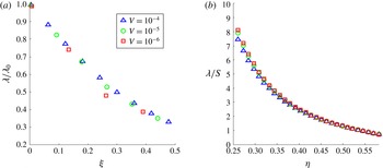
in Regime L. The scaled forces, as determined from numerical solutions of the Young–Laplace equation, are shown in figure 6. The scaling according to Regime S is depicted in figure 6(a), while the scaling according to Regime L is shown in figure 6(b). Data shown in figure 6(a) confirm that the curves for the capillary force ratio
 $\unicode[STIX]{x1D706}/\unicode[STIX]{x1D706}_{0}$
, for various values of the capillary bridge volume
 $V$
, are solely dependent on the scaled separation
 $\unicode[STIX]{x1D709}$
in Regime S for small values of
 $\unicode[STIX]{x1D709}$
. Data shown in figure 6(b) confirm that in Regime L the curves for the capillary force ratio
 $\unicode[STIX]{x1D706}/S$
, for various values of the capillary bridge volume
 $V$
, are solely dependent on the scaled separation
 $\unicode[STIX]{x1D702}$
for large values of
 $\unicode[STIX]{x1D702}$
.
Scaling regimes for the capillary force, represented by
 $\unicode[STIX]{x1D706}$
. (a) Regime S with scaling according to (4.13). (b) Regime L with scaling according to (4.14). Dimensionless capillary forces
 $\unicode[STIX]{x1D706}$
are based on numerical solutions of the Young–Laplace equation.

The predictions for the capillary force, represented by
 $\unicode[STIX]{x1D706}$
, as a function of the capillary bridge volume
 $V$
and the separation
 $S$
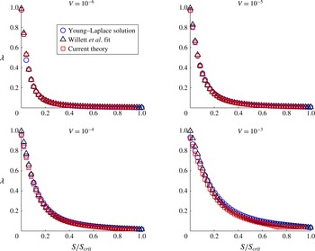
are compared quantitatively in figure 7 with the capillary force obtained from the numerical solutions of the Young–Laplace equation and with the fit by Willett et al. (Reference Willett, Adams, Johnson and Seville2000) (as reported in their appendix). The comprehensive fit by Willett et al. (Reference Willett, Adams, Johnson and Seville2000) has been selected for this comparison because it provides direct relations for the capillary force as a function of the capillary bridge volume and the separation. This is not the case for the toroidal approximation, for instance. The results according to the numerical solutions of the Young–Laplace equation have been obtained, using the interpolation method described in § 3.1 with the subset of solutions for which
 $Q\geqslant 0.25$
. In the presented results for the current theory the contact radius
 $Y_{c}$
has been determined approximately from the capillary bridge volume
 $V$
and the separation
 $S$
by (4.15).
Predictions of the dimensionless capillary force
 $\unicode[STIX]{x1D706}$
, as a function of the separation
 $S$
, according to the current theory for various volumes
 $V$
of the capillary bridge. Theoretical predictions are compared with the capillary forces as obtained from the numerical solution of the Young–Laplace equation and with the fit by Willett et al. (Reference Willett, Adams, Johnson and Seville2000). The critical separation
 $S_{crit}$
has been determined from (1.1).

Overall, the predictions according to the current theory show good agreement with the capillary forces obtained from the numerical solutions of the Young–Laplace equation for various values of the capillary bridge volume
 $V$
and separations
 $S$
up to the critical separation
 $S_{crit}$
(see figure 7). The deviations between the (effectively exact) capillary force from the numerical solution of the Young–Laplace equation and that according to the fit by Willett et al. (Reference Willett, Adams, Johnson and Seville2000) and by the current theory increase with increasing capillary bridge volume
 $V$
. For separations
 $S\leqslant 0.5S_{crit}$
, the (relative) deviation is less than 5 % for
 $V=10^{-6}$
and 10 % for
 $V=10^{-4}$
. For separations
 $S\geqslant 0.5S_{crit}$
, the (relative) deviations are larger but the capillary force is (very) small. For
 $V=10^{-3}$
, the fit by Willett et al. (Reference Willett, Adams, Johnson and Seville2000) gives a more accurate prediction (deviations up to 10 % for
 $S\leqslant 0.5S_{crit}$
) than the current theory (deviations up to 15 % for
 $S\leqslant 0.5S_{crit}$
). The fit by Willett et al. (Reference Willett, Adams, Johnson and Seville2000) has been formulated such that it is (also) accurate for larger capillary bridge volumes
 $V$
, while the current analytical theory is based on the assumption that the contact radius
 $Y_{c}$
(and hence also the capillary bridge volume
 $V$
) is small. Note that, for the current theory, results are only shown for separations that satisfy the rupture criterion corresponding to this theory, (4.17), while for the fit by Willett et al. (Reference Willett, Adams, Johnson and Seville2000) results are shown for separations
 $S$
that satisfy the rupture criterion of Lian et al. (Reference Lian, Thornton and Adams1993), (1.1).
5 Discussion
An analytical theory has been developed for properties of steady, axisymmetric capillary bridges between two identical, perfectly wettable, rigid spheres. In this theory the meridional profile of the capillary bridge is assumed to be a part of an ellipse. The accuracy of this geometrical assumption has been verified with numerical solutions of the governing Young–Laplace equation, according to which the mean curvature of the capillary bridge surface is constant in the absence of gravity.
In comparison to the toroidal approximation where the meridional profile is described by an arc, the current description by a part of an ellipse involves an additional, free geometrical parameter. Thus, an extra closure relation needs to be formulated. This is accomplished here by requiring that the mean curvature of the capillary bridge surface be equal at the neck and at the contact line. Hence, the current theory accounts for properties of the Young–Laplace equation.
The obtained closure relation
 $P=F(Q)$
, defined by (4.7), agrees well with results obtained from numerical solutions of the Young–Laplace equation for small capillary bridge volumes
 $V$
. An accurate Padé approximant of second order has been formulated in appendix A to describe the two branches of the inverse relation
 $Q=F^{-1}(P)$
.
An approximate equation for the contact radius
 $Y_{c}$
has been derived that involves the specified capillary bridge volume
 $V$
and the specified separation
 $S$
. Two regimes have been identified for solutions to this equation, Regime S corresponding to small separations
 $S$
and Regime L corresponding to large separations
 $S$
. A closed-form expression, equation (4.15), has been formulated analytically in appendix B for the approximate solution for the contact radius
 $Y_{c}$
as a function of the capillary bridge volume
 $V$
and the separation
 $S$
that combines these two regimes. As the inverse relation
 $Q=F^{-1}(P)$
has two branches, the observation by Erle et al. (Reference Erle, Dyson and Morrow1971) (based on numerical solutions of the Young–Laplace equation) that two solutions may exist for the meridional profile, for identical capillary bridge volume and interparticle separation, is obtained analytically here.
The closure relation
 $P=F(Q)$
exhibits a critical point
 $(Q^{\ast },P^{\ast })$
, which indicates a maximum achievable separation (at specified volume of the capillary bridge). Based on these considerations, a (quasi-static) rupture criterion, equation (4.17), has been obtained analytically that agrees (within 6 %) with that formulated by Lian et al. (Reference Lian, Thornton and Adams1993) from (many) numerical solutions of the governing Young–Laplace equation.
Finally, analytical expressions have been obtained for the capillary force as a function of the capillary bridge volume
 $V$
and the separation
 $S$
. For small values of the capillary bridge volume
 $V$
(say
 $V\leqslant 10^{-4}$
) the resulting predictions for the capillary forces agree well with those obtained from numerical solutions of the Young–Laplace equation and with the fit of Willett et al. (Reference Willett, Adams, Johnson and Seville2000). For larger values of the capillary bridge volume
 $V$
the current analytical predictions agree reasonably well.
For future studies, it is recommended to extend the current analytical approach to the case of non-zero wetting angles
 $\unicode[STIX]{x1D703}$
and to the case of spheres with different radii. For these two topics, results based on numerical solutions of the Young–Laplace equation and on the toroidal approximation have been reported by Lian et al. (Reference Lian, Thornton and Adams1993), Willett et al. (Reference Willett, Adams, Johnson and Seville2000), Harireche et al. (Reference Harireche, Faramarzi and Alani2013, Reference Harireche, Faramarzi and Alani2015) and Lian & Seville (Reference Lian and Seville2016).
Acknowledgements
The first author acknowledges support, in the form of a Van Gogh travel grant, by foundation Ammodo. The authors also acknowledge support from the French Research Network MeGe (Multiscale and Multi-physics Couplings in Geo-environmental Mechanics; GDR CNRS 3176, 2012–2015).
Appendix A
The closure relation
 $P=F(Q)$
between
 $P$
and
 $Q$
corresponding to (4.7) has to be inverted in the calculation of the capillary force (represented by
 $\unicode[STIX]{x1D706}$
) from the specified capillary bridge volume
 $V$
and the separation
 $S$
, see § 4.5. Two branches are present, for
 $Q\leqslant Q^{\ast }$
and for
 $Q\geqslant Q^{\ast }$
, as shown in figure 4(a). To accomplish this inversion in a simple, analytical manner, the relation
 $P=F(Q)$
given by (4.7) is approximated by a Padé approximant of second order for both numerator and denominator:
 $$\begin{eqnarray}\displaystyle P\cong J(Q)\equiv \frac{K_{2}Q^{2}+K_{1}Q+K_{0}}{Q^{2}+L_{1}Q+L_{0}}. & & \displaystyle\end{eqnarray}$$
This choice for the Padé approximant has been adopted because it leads to a quadratic equation for
 $Q$
(represented by (A 5), as shown below) that can be solved easily for the two branches of
 $Q=F^{-1}(P)$
.
The function
 $F(Q)$
shown in figure 4(a) has the features that it equals zero at
 $Q=0$
and at
 $Q=1$
, it has a maximum
 $P^{\ast }$
for
 $Q=Q^{\ast }$
and a slope of
 $-1$
at
 $Q=1$
, consistent with the toroidal approximation. According to the developed theoretical relation (4.7),
 $Q^{\ast }\cong 0.338$
and
 $P^{\ast }\cong 0.412$
. The five coefficients
 $K_{2}$
,
 $K_{1}$
,
 $K_{0}$
,
 $L_{1}$
and
 $L_{0}$
present in the Padé approximant defined by (A 1) are therefore determined from the five requirements
 $$\begin{eqnarray}\displaystyle J(0)=0,\quad J(1)=0,\quad J(Q^{\ast })=P^{\ast },\quad J^{\prime }(Q^{\ast })=0,\quad J^{\prime }(1)=-1, & & \displaystyle\end{eqnarray}$$
where
 $J^{\prime }(Q)=\text{d}J(Q)/\text{d}Q$
.
After some algebra it follows that
 $$\begin{eqnarray}\displaystyle \left.\begin{array}{@{}c@{}}\displaystyle K_{0}=0,\quad K_{1}=\frac{P^{\ast }(1-Q^{\ast })^{2}}{P^{\ast }-(1-Q^{\ast })^{2}},\quad K_{2}=\frac{-P^{\ast }(1-Q^{\ast })^{2}}{P^{\ast }-(1-Q^{\ast })^{2}},\\ \displaystyle L_{0}=\frac{P^{\ast }Q^{\ast 2}}{P^{\ast }-(1-Q^{\ast })^{2}},\quad L_{1}=-\frac{2P^{\ast }Q^{\ast }-(1-Q^{\ast })^{2}}{P^{\ast }-(1-Q^{\ast })^{2}}\end{array}\right\} & & \displaystyle\end{eqnarray}$$
and hence
 $J(Q)$
is given by
 $$\begin{eqnarray}\displaystyle J(Q)=\frac{P^{\ast }(1-Q^{\ast })^{2}Q(1-Q)}{[P^{\ast }-(1-Q^{\ast })^{2}]Q^{2}+[(1-Q^{\ast })^{2}-2P^{\ast }Q^{\ast }]Q+P^{\ast }Q^{\ast 2}}. & & \displaystyle\end{eqnarray}$$
The corresponding two (approximate) branches of the inverse function
 $Q=F^{-1}(P)$
are therefore given by the two solutions of the quadratic equation for
 $Q$
:
 $$\begin{eqnarray}\displaystyle 0=[(P^{\ast }-P)(1-Q^{\ast })^{2}+PP^{\ast }]Q^{2}+[(P-P^{\ast })(1-Q^{\ast })^{2}-2PP^{\ast }Q^{\ast }]Q+[PP^{\ast }Q^{\ast 2}]. & & \displaystyle \nonumber\\ \displaystyle & & \displaystyle\end{eqnarray}$$
It is readily verified that the discriminant of this quadratic equation is non-negative for
 $P\leqslant P^{\ast }$
and
 $0\leqslant Q\leqslant 1$
.
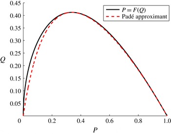
The function
 $F(Q)$
defined by (4.7) and the Padé approximant
 $J(Q)$
defined by (A 4) are compared in figure 8. This figure shows that for the branch with
 $Q\geqslant Q^{\ast }$
the function
 $F(Q)$
is very well approximated by
 $J(Q)$
. The deviation for the less relevant branch with
 $Q\leqslant Q^{\ast }$
is somewhat larger.


Appendix B
Real, positive solutions for the contact radius
 $Y_{c}$
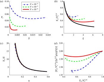
of the quartic equation (4.12) that have been obtained numerically are shown in figure 9(a) as a function of the separation
 $S$
for various values of the capillary bridge volume
 $V$
. The analytical solutions for
 $Y_{c}$
given in § 4.3 for small separations
 $S$
(Regime S, described by (4.13)) and that for large separations
 $S$
(Regime L, described by (4.14)) result in different scaling relations for the contact radius
 $Y_{c}$
as a function of the capillary bridge volume
 $V$
and the separation
 $S$
. These scaling relations are shown in figure 9(b,c), where the theoretical relations are also depicted.
(a) Numerical solutions
 $Y_{c}$
of the quartic equation (4.12) as a function of separation
 $S$
, for various capillary bridge volumes
 $V$
. (b) Numerical solutions for
 $Y_{c}$
, rescaled according to the scaling relation in (4.13) for Regime S that is valid for small separations
 $S$
; also shown by a solid black line is the theoretical relation in (4.13). (c) Numerical solutions for
 $Y_{c}$
, rescaled according to the scaling relation in (4.14) for Regime L that is valid for large separations
 $S$
; also shown by a solid black line is the theoretical relation in (4.14). (d) Verification of the combined matching of solutions, according to which the quantity along the vertical axis should be constant and equal to 2, see (B 5).

In figure 9(b) the results for
 $Y_{c}$
, scaled with
 $V_{s}^{1/4}$
(recall that
 $V_{s}$
is defined in (4.11)) as suggested by (4.13), collapse to a single curve for different values of the capillary bridge volume
 $V$
for small values of the scaled separation
 $\unicode[STIX]{x1D709}$
(say for
 $\unicode[STIX]{x1D709}\leqslant 0.5$
;
 $\unicode[STIX]{x1D709}$
is defined in (4.13)). Also shown here (in black) is the theoretical relation
 $f(\unicode[STIX]{x1D709})$
, defined in (4.13), that describes these results accurately.
In figure 9(c) the results for
 $Y_{c}$
, scaled with
 $S$
as suggested by (4.14), collapse to a single curve for different values of the capillary bridge volume
 $V$
for large values of the scaled separation
 $\unicode[STIX]{x1D702}$
(say for
 $\unicode[STIX]{x1D702}\geqslant 0.1$
;
 $\unicode[STIX]{x1D702}$
is defined in (4.14)). Also shown here (in black) is the theoretical relation
 $g(\unicode[STIX]{x1D702})$
, defined in (4.14), that describes these results accurately. Data are shown here only for
 $\unicode[STIX]{x1D702}\geqslant 0.1$
, because the theoretical relation and the numerical data diverge as
 $\unicode[STIX]{x1D702}\rightarrow 0$
.
To match the solutions valid for these two regimes to a generally valid approximate solution, ‘correction factors’
 $\unicode[STIX]{x1D70C}$
and
 $\unicode[STIX]{x1D70F}$
are introduced:
 $$\begin{eqnarray}\displaystyle \frac{Y_{c}}{V_{s}^{1/4}}=\unicode[STIX]{x1D70C}(\unicode[STIX]{x1D702})f(\unicode[STIX]{x1D709}),\quad \frac{Y_{c}}{S}=\unicode[STIX]{x1D70F}(\unicode[STIX]{x1D709})g(\unicode[STIX]{x1D702}). & & \displaystyle\end{eqnarray}$$
It has been postulated in (B 1) that these forms involve a separation of variables, since
 $\unicode[STIX]{x1D70C}=\unicode[STIX]{x1D70C}(\unicode[STIX]{x1D702})$
and
 $\unicode[STIX]{x1D70F}=\unicode[STIX]{x1D70F}(\unicode[STIX]{x1D709})$
. For consistency of both relations in (B 1), we have
 $$\begin{eqnarray}\displaystyle V_{s}^{1/4}\unicode[STIX]{x1D70C}(\unicode[STIX]{x1D702})f(\unicode[STIX]{x1D709})=Y_{c}=S\unicode[STIX]{x1D70F}(\unicode[STIX]{x1D709})g(\unicode[STIX]{x1D702}). & & \displaystyle\end{eqnarray}$$
From the definitions of
 $\unicode[STIX]{x1D709}$
and
 $\unicode[STIX]{x1D702}$
in (4.13) and (4.14),
 $V_{s}$
and
 $S$
can be expressed in terms of
 $\unicode[STIX]{x1D709}$
and
 $\unicode[STIX]{x1D702}$
as
 $V_{s}=(\unicode[STIX]{x1D702}/\unicode[STIX]{x1D709})^{6}$
and
 $S=\unicode[STIX]{x1D702}^{3}/\unicode[STIX]{x1D709}^{2}$
. By substituting these relations into (B 2) and separating the variables
 $\unicode[STIX]{x1D709}$
and
 $\unicode[STIX]{x1D702}$
, it follows that
 $$\begin{eqnarray}\displaystyle \unicode[STIX]{x1D702}^{-3/2}\frac{\unicode[STIX]{x1D70C}(\unicode[STIX]{x1D702})}{g(\unicode[STIX]{x1D702})}=\unicode[STIX]{x1D709}^{-1/2}\frac{\unicode[STIX]{x1D70F}(\unicode[STIX]{x1D709})}{f(\unicode[STIX]{x1D709})}=D. & & \displaystyle\end{eqnarray}$$
Note that
 $D$
is a constant, because it is simultaneously equal to a function solely of
 $\unicode[STIX]{x1D709}$
and to a function solely of
 $\unicode[STIX]{x1D702}$
. Hence
 $$\begin{eqnarray}\displaystyle \unicode[STIX]{x1D70C}(\unicode[STIX]{x1D702})=D\unicode[STIX]{x1D702}^{3/2}g(\unicode[STIX]{x1D702}),\quad \unicode[STIX]{x1D70F}(\unicode[STIX]{x1D709})=D\unicode[STIX]{x1D709}^{1/2}f(\unicode[STIX]{x1D709}). & & \displaystyle\end{eqnarray}$$
The two scaling relations for
 $Y_{c}$
, including the results for the correction factors
 $\unicode[STIX]{x1D70C}$
and
 $\unicode[STIX]{x1D70F}$
, become
 $$\begin{eqnarray}\displaystyle \frac{Y_{c}}{V_{s}^{1/4}}=D\unicode[STIX]{x1D702}^{3/2}g(\unicode[STIX]{x1D702})f(\unicode[STIX]{x1D709}),\quad \frac{Y_{c}}{S}=D\unicode[STIX]{x1D709}^{1/2}f(\unicode[STIX]{x1D709})g(\unicode[STIX]{x1D702}). & & \displaystyle\end{eqnarray}$$
The description by (4.13) is appropriate for small
 $\unicode[STIX]{x1D709}$
(see figure 9
b), while the description by (4.14) is appropriate for large
 $\unicode[STIX]{x1D702}$
(see figure 9
c). The constant
 $D$
is determined from the condition that the multiplicative correction
 $D\unicode[STIX]{x1D702}^{3/2}g(\unicode[STIX]{x1D702})$
to
 $f(\unicode[STIX]{x1D709})$
becomes equal to one for small values of
 $\unicode[STIX]{x1D702}$
and that the multiplicative correction
 $D\unicode[STIX]{x1D709}^{1/2}f(\unicode[STIX]{x1D709})$
to
 $g(\unicode[STIX]{x1D702})$
becomes equal to one for large values of
 $\unicode[STIX]{x1D709}$
:
 $$\begin{eqnarray}\displaystyle \lim _{\unicode[STIX]{x1D702}\rightarrow 0}(D\unicode[STIX]{x1D702}^{3/2}g(\unicode[STIX]{x1D702}))=1=\lim _{\unicode[STIX]{x1D709}\rightarrow \infty }(D\unicode[STIX]{x1D709}^{1/2}f(\unicode[STIX]{x1D709})). & & \displaystyle\end{eqnarray}$$
Both requirements in (B 6) result in
 $D=2$
.
According to this description in (B 5) the quantity
 $(Y_{c}/V_{s}^{1/4})/(\unicode[STIX]{x1D702}^{3/2}g(\unicode[STIX]{x1D702})f(\unicode[STIX]{x1D709}))$
should be constant and equal to
 $D=2$
. As shown in figure 9(d), this is indeed the case (within 1.5 %). Hence, the (real, positive) solution
 $Y_{c}$
of the quartic equation (4.12) for the capillary bridge volume
 $V$
is well described by (either of) the expressions in (B 5) for small capillary bridge volumes
 $V$
and small separations
 $S$
.
The final expression for the non-negative solution
 $Y_{c}$
of (4.12) as a function of the capillary bridge volume
 $V$
and the separation
 $S$
is given in a form that is less susceptible to round-off errors as
 $$\begin{eqnarray}\displaystyle Y_{c}=2S^{3/2}V_{s}^{-1/4}f(\unicode[STIX]{x1D709})g(\unicode[STIX]{x1D702}). & & \displaystyle\end{eqnarray}$$