2 DNS model

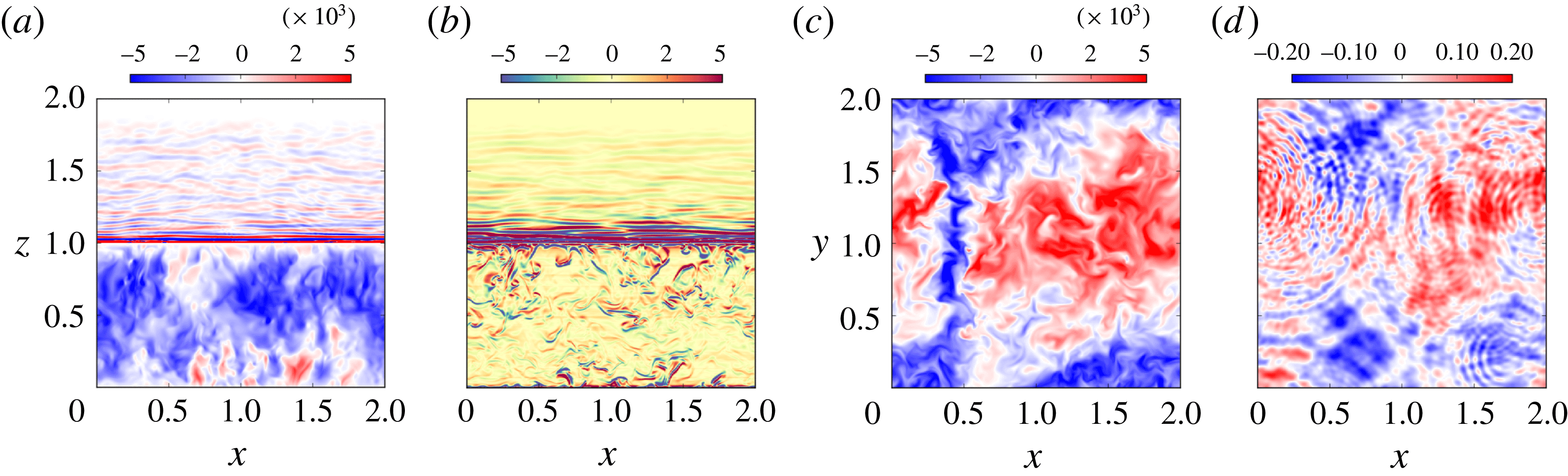
The fluid model we use is similar to the one used in Couston et al. (Reference Couston, Lecoanet, Favier and Le Bars2017), though here it is three-dimensional (figure 1). We solve the Navier–Stokes equations under the Boussinesq approximation, i.e. the fluid density is $\unicode[STIX]{x1D70C}=\unicode[STIX]{x1D70C}_{0}+\unicode[STIX]{x1D6FF}\unicode[STIX]{x1D70C}$ , where $\unicode[STIX]{x1D70C}_{0}$ is the (constant) reference density and $\unicode[STIX]{x1D6FF}\unicode[STIX]{x1D70C}\ll \unicode[STIX]{x1D70C}_{0}$ are small variations due to temperature fluctuations. We consider constant kinematic viscosity $\unicode[STIX]{x1D708}$ , acceleration due to gravity $g$ and thermal diffusivity $\unicode[STIX]{x1D705}$ . The governing equations for the velocity $\boldsymbol{u}=(u,v,w)$ and temperature $T$ in a Cartesian $(x,y,z)$ frame of reference ( $\hat{\boldsymbol{z}}$ is the upward-pointing unit vector of the $z$ -axis) read

(2.1a ) $$\begin{eqnarray}\displaystyle & \displaystyle \unicode[STIX]{x2202}_{t}\boldsymbol{u}+(\boldsymbol{u}\boldsymbol{\cdot }\unicode[STIX]{x1D735})\boldsymbol{u}=-\unicode[STIX]{x1D735}p+\unicode[STIX]{x1D708}\unicode[STIX]{x1D6FB}^{2}\boldsymbol{u}-g\unicode[STIX]{x1D6FF}\unicode[STIX]{x1D70C}/\unicode[STIX]{x1D70C}_{0}\hat{\boldsymbol{z}}-\boldsymbol{u}/\unicode[STIX]{x1D70F}, & \displaystyle\end{eqnarray}$$

(2.1b ) $$\begin{eqnarray}\displaystyle & \displaystyle \unicode[STIX]{x2202}_{t}T+(\boldsymbol{u}\boldsymbol{\cdot }\unicode[STIX]{x1D735})T=\unicode[STIX]{x1D705}\unicode[STIX]{x1D6FB}^{2}T, & \displaystyle\end{eqnarray}$$

(2.1c ) $$\begin{eqnarray}\displaystyle & \displaystyle \unicode[STIX]{x1D735}\boldsymbol{\cdot }\boldsymbol{u}=0, & \displaystyle\end{eqnarray}$$

$p$

$-\boldsymbol{u}/\unicode[STIX]{x1D70F}$

$\unicode[STIX]{x1D6FF}\unicode[STIX]{x1D70C}$

$T$

(2.2) $$\begin{eqnarray}\unicode[STIX]{x1D6FF}\unicode[STIX]{x1D70C}/\unicode[STIX]{x1D70C}_{0}=-\unicode[STIX]{x1D6FC}(T)(T-T_{i})=-\unicode[STIX]{x1D6FC}_{s}\mathsf{H}(T-T_{i})(T-T_{i})+\unicode[STIX]{x1D6FC}_{s}{\mathcal{S}}\mathsf{H}(T_{i}-T)(T-T_{i}),\end{eqnarray}$$

with $\mathsf{H}$ the Heaviside function; $\unicode[STIX]{x1D6FC}_{s}>0$ is the thermal expansion coefficient for $T>T_{i}$ , with $T_{i}$ the inversion temperature at which the density anomaly $\unicode[STIX]{x1D6FF}\unicode[STIX]{x1D70C}/\unicode[STIX]{x1D70C}_{0}=0$ is maximum, and ${\mathcal{S}}>0$ is the stiffness parameter. We assume periodicity in the horizontal directions and impose free-slip and fixed temperatures conditions on the top ( $T=T_{t}$ ) and bottom boundaries ( $T=T_{b}$ ), with $T_{b}>T_{i}>T_{t}$ (note that the use of no-slip boundary condition at the bottom boundary is not expected to significantly change the results at the interface). Then, because (2.2) is non-monotonic, the lower part of the fluid is convectively unstable, the upper part is stably stratified and ${\mathcal{S}}$ indicates how sharp or ‘stiff’ the transition is at the interface (Couston et al. Reference Couston, Lecoanet, Favier and Le Bars2017).

Figure 1.

Snapshots of (a) $w(y=0)$ , (b)  $T_{z}(y=0)-\overline{T}_{z}$ (overbar denotes the horizontal average), (c)  $w(z=0.7)$ , (d)  $w(z=1.3)$ for case $C_{8}^{400}$ at steady-state. Variables in the wave region ( $z>1$ ) in (a), (b) have been multiplied by $10^{4},10^{3}$ , respectively. A movie is available as Supplementary Material at https://doi.org/10.1017/jfm.2018.669.

We use the characteristic length scale $H$ , the thermal diffusion time $H^{2}/\unicode[STIX]{x1D705}$ , and the temperature difference $\unicode[STIX]{x0394}T=T_{b}-T_{i}$ in order to define the non-dimensional variables:

(2.3a-f ) $$\begin{eqnarray}(\tilde{x},{\tilde{y}},\tilde{z})=\frac{(x,y,z)}{H},\quad \tilde{t}=\frac{t\unicode[STIX]{x1D705}}{H^{2}},\quad \tilde{\boldsymbol{u}}=\frac{\boldsymbol{u}H}{\unicode[STIX]{x1D705}},\quad \tilde{T}=\frac{T-T_{i}}{\unicode[STIX]{x0394}T},\quad \tilde{p}=\frac{pH^{2}}{\unicode[STIX]{x1D705}^{2}},\quad \tilde{\unicode[STIX]{x1D70C}}=\frac{\unicode[STIX]{x1D6FF}\unicode[STIX]{x1D70C}}{\unicode[STIX]{x1D70C}_{0}\unicode[STIX]{x1D6FC}_{s}\unicode[STIX]{x0394}T}.\end{eqnarray}$$

Substituting (2.3) in (2.1)–(2.2) and dropping tildes we obtain the dimensionless equations

(2.4a ) $$\begin{eqnarray}\displaystyle & \displaystyle \unicode[STIX]{x2202}_{t}\boldsymbol{u}+(\boldsymbol{u}\boldsymbol{\cdot }\unicode[STIX]{x1D735})\boldsymbol{u}=-\unicode[STIX]{x1D735}p+Pr\unicode[STIX]{x1D6FB}^{2}\boldsymbol{u}-PrRa\unicode[STIX]{x1D70C}\hat{z}-\boldsymbol{u}/\unicode[STIX]{x1D70F}, & \displaystyle\end{eqnarray}$$

(2.4b ) $$\begin{eqnarray}\displaystyle & \displaystyle \unicode[STIX]{x2202}_{t}T+(\boldsymbol{u}\boldsymbol{\cdot }\unicode[STIX]{x1D735})T=\unicode[STIX]{x1D6FB}^{2}T, & \displaystyle\end{eqnarray}$$

(2.4c ) $$\begin{eqnarray}\displaystyle & \displaystyle \unicode[STIX]{x1D735}\boldsymbol{\cdot }\boldsymbol{u}=0, & \displaystyle\end{eqnarray}$$

(2.4d ) $$\begin{eqnarray}\displaystyle & \displaystyle \unicode[STIX]{x1D70C}=-T\mathsf{H}(T)+{\mathcal{S}}T\mathsf{H}(-T), & \displaystyle\end{eqnarray}$$

$Pr=\unicode[STIX]{x1D708}/\unicode[STIX]{x1D705}$

$Ra=\unicode[STIX]{x1D6FC}_{s}g\unicode[STIX]{x0394}TH^{3}/(\unicode[STIX]{x1D708}\unicode[STIX]{x1D705})$

$L_{x},L_{y},L_{z}$

$x,y,z$

$T_{top}<0$

$z=L_{z}$

$T=1$

$z=0$

$T=0$

$z$

$\unicode[STIX]{x1D70F}^{-1}(z)=0.5f_{N^{\ast }}\{\tanh [(z-L_{z}+0.15)/0.05]+1\}$

$f_{N^{\ast }}$

We solve (2.4) using the open-source pseudo-spectral code DEDALUS (Burns et al. Reference Burns, Vasil, Oishi, Lecoanet and Brown2018). We are interested in DNS results at statistical steady state and in the limit of fully turbulent convection (large $Ra$ ) and strong stable stratification (large ${\mathcal{S}}$ ). For ease of presentation, we want the convection to extend from $z=0$ to $z=z_{i}\approx 1$ at thermal equilibrium, i.e. such that $H$ is approximately the size of the convection zone in dimensional variables and $Ra$ is the effective Rayleigh number of the convection. $z_{i}$ is an output of our simulations, but it can be controlled by iteratively adjusting $T_{top}$ (all other parameters fixed). At leading order, $z_{i}\approx 1$ when $T_{top}$ is chosen such that the measured heat flux $Q=\overline{wT-T_{z}}$ in the convection (overbar denotes the horizontal average) equals the expected diffusive heat flux of the stable region ${\approx}-T_{top}/(L_{z}-z_{i})$ with $z_{i}=1$ . Because $Q$ in the convection zone changes with $T_{top}$ , finding $T_{top}$ is carried out iteratively. We fix all problem parameters except $T_{top}$ , make an initial guess for $T_{top}$ , and run a simulation for a few convective turnover times, initialized with a temperature of $T=(1-z)\mathsf{H}(1-z)+T_{top}(z-1)/(L_{z}-1)\mathsf{H}(z-1)$ plus low-amplitude noise. We then update our guess for $T_{top}$ using $T_{top}=-Q(L_{z}-z_{i})$ with $z_{i}=1$ , where $Q$ is the average heat flux at $z=0$ , and we reiterate until $T_{top}$ does not change by more than about 10 %. The final $T_{top}$ gives an estimate for the buoyancy frequency $f_{N^{\ast }}=\sqrt{-PrRa{\mathcal{S}}T_{top}/(L_{z}-1)}/(2\unicode[STIX]{x03C0})$ used in the expression for the damping term $\unicode[STIX]{x1D70F}$ in (2.4a ). The actual buoyancy frequency $f_{N}=N/(2\unicode[STIX]{x03C0})$ is computed using $N=\sqrt{PrRa{\mathcal{S}}Q}$ with $Q$ averaged from $z=0$ to $z=1$ and over the simulation time $\unicode[STIX]{x0394}t$ . In all the simulations, we set $L_{x}=L_{y}=L_{z}=L$ with $L=2$ or $L=3$ . Therefore, the ratio between the horizontal and vertical extent of the convective zone is larger than 2, which ensures that confinement effects associated with the horizontal periodic boundary conditions are not dominating the dynamics. 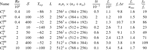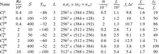We set $Pr=1$ for simplicity. Input and output parameters of the eight simulations discussed in this paper are reported in table 1.

The variables of interest include the kinetic energy spectrum and the energy flux spectrum. The kinetic energy per unit surface area and unit (thermal) time reads

(2.5) $$\begin{eqnarray}K(z)=\int \frac{|\boldsymbol{u}|^{2}}{2}\frac{\text{d}x\,\text{d}y\,\text{d}t}{L^{2}\unicode[STIX]{x0394}t}\approx \mathop{\sum }_{f,k_{\bot }}\frac{|\hat{\boldsymbol{u}}|^{2}}{2\unicode[STIX]{x1D6FF}f\unicode[STIX]{x1D6FF}k_{\bot }}\unicode[STIX]{x1D6FF}f\unicode[STIX]{x1D6FF}k_{\bot }\equiv \mathop{\sum }_{f,k_{\bot }}\,\text{d}K\unicode[STIX]{x1D6FF}f\unicode[STIX]{x1D6FF}k_{\bot }\approx \int \frac{\unicode[STIX]{x2202}^{2}K}{\unicode[STIX]{x2202}f\unicode[STIX]{x2202}k_{\bot }}\,\text{d}f\,\text{d}k_{\bot },\end{eqnarray}$$

with hat denoting the Fourier transform in $(x,y,t)$ , $\unicode[STIX]{x0394}t$ the period over which results are integrated in time, $k_{\bot }$ and $f$ are the horizontal wavenumber and frequency, $\unicode[STIX]{x1D6FF}k_{\bot }$ and $\unicode[STIX]{x1D6FF}f$ are the unit increments in spectral space, and $\text{d}K$ is the discrete version of the kinetic energy spectrum $\unicode[STIX]{x2202}^{2}K/\unicode[STIX]{x2202}f\unicode[STIX]{x2202}k_{\bot }$ . Similarly, we define the $z$ -dependent vertical energy flux as

(2.6) $$\begin{eqnarray}F(z)=\int wp\frac{\text{d}x\,\text{d}y\,\text{d}t}{L^{2}\unicode[STIX]{x0394}t}\approx \mathop{\sum }_{f,k_{\bot }}\frac{\text{Re}({\hat{w}}\hat{p}^{\ast })}{\unicode[STIX]{x1D6FF}f\unicode[STIX]{x1D6FF}k_{\bot }}\unicode[STIX]{x1D6FF}f\unicode[STIX]{x1D6FF}k_{\bot }\equiv \mathop{\sum }_{f,k_{\bot }}\,\text{d}F\unicode[STIX]{x1D6FF}f\unicode[STIX]{x1D6FF}k_{\bot }\approx \int \frac{\unicode[STIX]{x2202}^{2}F}{\unicode[STIX]{x2202}f\unicode[STIX]{x2202}k_{\bot }}\,\text{d}f\,\text{d}k_{\bot },\end{eqnarray}$$

where $\ast$ denotes the complex conjugate, $\text{d}F$ is the discrete energy flux spectrum and $\text{Re}$ denotes the real part. Note that throughout this paper, we assume isotropic motions in the $x,y$ directions and express variables in spectral space in terms of the average horizontal wavenumber $k_{\bot }=(k_{x}^{2}+k_{y}^{2})^{1/2}$ (with $k_{x},k_{y}$ the wavenumbers in the $x,y$ directions). Thus, $|\hat{\boldsymbol{u}}|^{2}\equiv |\hat{\boldsymbol{u}}(k_{\bot })|^{2}$ is the azimuthal average of $|\hat{\boldsymbol{u}}(k_{x},k_{y})|^{2}$ and $\text{Re}({\hat{w}}\hat{p}^{\ast })$ is the azimuthal average of $\text{Re}[{\hat{w}}(k_{x},k_{y})\hat{p}^{\ast }(k_{x},k_{y})]$ based on the modulus of vector $(k_{x},k_{y})$ , i.e. averaging over all orientations. We apply a Hann windowing function to all variables before taking the time Fourier transform and we discard the modes $f=0$ and $k_{\bot }=0$ from the spectra.

Table 1.

Simulation parameters: number of Fourier modes $n_{x},n_{y}$ in the $x,y$ directions, Chebyshev modes $n_{zl}/n_{zu}$ in the lower/upper regions of the compound $z$ basis (stitched at $z=1.2$ ), typical time steps $\unicode[STIX]{x1D6FF}t$ , best-fit convective frequency $f_{c}$ for ${\mathcal{A}}=30$ (cf. § 4.2), time $f_{c}\unicode[STIX]{x0394}t$ of data collection, convective velocity $u_{rms}$ and Brunt–Väisälä frequency $f_{N}$ . $Pr=1$ in all simulations.

3 Theoretical prediction

We now describe a heuristic model which predicts the wave energy flux spectrum at the interface, $F^{i}(f,k_{\bot })$ , between the convective and stably stratified layers. This is based on the calculation in Lecoanet & Quataert (Reference Lecoanet and Quataert2013) (specifically, the ‘discontinuous’ $N^{2}$ case), which itself is based on the earlier calculation in Goldreich & Kumar (Reference Goldreich and Kumar1990). We first assume that turbulence driven by the convection can be decomposed into ‘eddies’, each of which has a characteristic length $h$ and velocity $u_{h}$ . The largest such ‘eddy’ is the large-scale circulation of the convection, which has length $\ell _{c}=2\unicode[STIX]{x03C0}/k_{c}$ and velocity $u_{c}$ . We imagine this large-scale circulation represents the injection scale of a Kolmogorov turbulent cascade and to recover the $k^{-5/3}$ energy spectrum ( $k$ is the three-dimensional wavenumber), we require that the typical velocity of eddies with size $h$ scales like $u_{h}/u_{c}=(h/\ell _{c})^{1/3}$ . We assume each eddy is coherent for an eddy turnover time $\unicode[STIX]{x1D70F}_{h}=h/u_{h}$ , which implies that the power spectrum in the convection zone is peaked along the curve $\unicode[STIX]{x1D70F}_{h}f_{c}=(h/\ell _{c})^{2/3}$ . This ignores the fact that small eddies can be advected over their size $h$ on time scales shorter than $\unicode[STIX]{x1D70F}_{h}$ by large-scale motions. This set of assumptions is very simplistic, but allows a theoretical derivation of the wave energy flux spectrum.

In this hypothesis, the waves are generated by Reynolds stresses within the convection zone. We calculate the waves generated by a single eddy with size $h$ and corresponding turnover time $\unicode[STIX]{x1D70F}_{h}$ , and then sum up the wave energy flux over all eddies. An eddy with size $h$ and turnover time $\unicode[STIX]{x1D70F}_{h}$ can only efficiently excite a wave with frequency $f$ and wavenumber $k_{\bot }$ if both

(3.1a,b ) $$\begin{eqnarray}f\leqslant \unicode[STIX]{x1D70F}_{h}^{-1},\quad \ell _{c}(k_{\bot }/2\unicode[STIX]{x03C0})\leqslant \ell _{c}/h=(\unicode[STIX]{x1D70F}_{h}f_{c})^{-3/2}.\end{eqnarray}$$

This is because we assume the spectral representation of an eddy’s velocity field is peaked at wavenumbers around $2\unicode[STIX]{x03C0}/h$ and decreases exponentially at higher wavenumbers due to analyticity (and similarly for the temporal spectrum with time scale $\unicode[STIX]{x1D70F}_{h}$ ). Waves with $f>\unicode[STIX]{x1D70F}_{h}^{-1}$ or $k_{\bot }>2\unicode[STIX]{x03C0}/h$ then have exponentially small coupling to eddies of size $h$ .

To connect the properties of the convection to the waves, one can write an equation for the wave velocity as a function of turbulent stresses as (Lecoanet & Quataert Reference Lecoanet and Quataert2013),

(3.2) $$\begin{eqnarray}\unicode[STIX]{x1D6FB}^{2}\unicode[STIX]{x2202}_{t}^{2}w+N^{2}(z)(\unicode[STIX]{x2202}_{x}^{2}+\unicode[STIX]{x2202}_{y}^{2})w=S,\end{eqnarray}$$

where $S$ is related to the Reynolds stresses associated with convective eddies. Note that we have neglected the effects of diffusion in the excitation process and that we have also neglected thermal stresses within the convection zone (as in Lecoanet et al. Reference Lecoanet, Le Bars, Burns, Vasil, Brown, Quataert and Oishi2015). Lecoanet & Quataert (Reference Lecoanet and Quataert2013) derive the internal waves’ Green’s function from this equation assuming $N^{2}(z)$ is constant in the convective and stably stratified regions, and discontinuous at the interface. One can then estimate the convolution of this Green’s function with the Reynolds stress of an eddy to find that the wave energy flux from eddies of size $h$ is

(3.3) $$\begin{eqnarray}\frac{\text{d}F^{i}}{\text{d}\log k_{\bot }\,\text{d}\log f\,\text{d}\log h}={\mathcal{A}}u_{h}^{3}\frac{f_{c}}{f_{N}}\frac{f}{f_{c}}\left(\frac{k_{\bot }h}{2\unicode[STIX]{x03C0}}\right)^{4}={\mathcal{A}}u_{c}^{3}\frac{f_{c}}{f_{N}}\frac{f}{f_{c}}\frac{h}{\ell _{c}}\left(\frac{k_{\bot }h}{2\unicode[STIX]{x03C0}}\right)^{4},\end{eqnarray}$$

with ${\mathcal{A}}$ a multiplicative constant, assumed universal, i.e. independent of all problem, wave or eddy parameters. To calculate the wave energy flux for a given frequency and wavenumber, we must sum up excitation from all eddies which satisfy (3.1). Because of the strong dependence on the eddy size in (3.3), the wave energy flux is dominated by the largest possible eddies which can excite a wave. The wave energy flux depends on whether the wave frequency is higher or lower than the frequency of the largest generating eddy $f^{\ast }(k_{\bot })=f_{c}[\ell _{c}k_{\bot }/(2\unicode[STIX]{x03C0})]^{2/3}$ . Waves with $(k_{\bot },f)$ satisfying $f<f^{\ast }(k_{\bot })$ are not observed in the bulk of the stable region in DNS because they are strongly dissipated (see discussion after (3.5)), so we neglect their contribution to the energy flux in the theory. The expression for the flux of the waves that matter away from the interface, i.e. with frequency $f>f_{c}[\ell _{c}k_{\bot }/(2\unicode[STIX]{x03C0})]^{2/3}$ , is

(3.4) $$\begin{eqnarray}\frac{\text{d}F^{i}}{\text{d}\log k_{\bot }\text{d}\log f}={\mathcal{A}}u_{c}^{3}\frac{f_{c}}{f_{N}}\left(\frac{f}{f_{c}}\right)^{-13/2}\left(\frac{k_{\bot }\ell _{c}}{2\unicode[STIX]{x03C0}}\right)^{4}.\end{eqnarray}$$

We recall that (3.4) is a prediction for the energy flux spectrum of inviscid propagating wave modes at the interface between convective and stably stratified regions. In the DNS, however, the energy flux at the interface has contributions from both inviscid and viscid wave modes and overshooting plumes, such that it is not expected to match the prediction (3.4). In order to avoid this discrepancy, we compare the theory with DNS away from the interface, where overshooting plumes and strongly viscous modes can be neglected.

In order to extend the expression for the flux (3.4) at the interface to an expression valid in all of the stable layer we derive a wave decay rate from the linear equation

(3.5) $$\begin{eqnarray}(\unicode[STIX]{x2202}_{t}-\unicode[STIX]{x1D6FB}^{2})^{2}\unicode[STIX]{x1D6FB}^{2}w+N^{2}\left(\unicode[STIX]{x2202}_{x}^{2}+\unicode[STIX]{x2202}_{y}^{2}\right)w=0,\end{eqnarray}$$

valid for $Pr=1$ . Note this differs from the inviscid equation (3.2) used to derive the wave flux at the interface. Substituting a plane wave solution $w\sim \text{e}^{\text{i}(k_{x}x+k_{y}y-\unicode[STIX]{x1D714}t)}\text{e}^{(\text{i}k_{z}-\unicode[STIX]{x1D6FE})z}$ with $\unicode[STIX]{x1D714}>0$ in (3.5) yields a cubic complex equation for $(\text{i}k_{z}-\unicode[STIX]{x1D6FE})^{2}$ whose six roots can be written in closed form. We assume that motions in the stable layer are dominated by waves propagating upward, i.e. with group velocity $C_{gz}=\unicode[STIX]{x2202}\unicode[STIX]{x1D714}/\unicode[STIX]{x2202}k_{z}>0$ , and whose amplitudes decrease with $z$ . One of the three roots $(k_{zj},\unicode[STIX]{x1D6FE}_{j})$ with $C_{gzj}>0$ has a much smaller decay rate $\unicode[STIX]{x1D6FE}_{j}$ than the other two, such that it is expected to be the dominant contribution to upward-propagating and decaying waves in DNS. Unsurprisingly, this solution is the ‘full-dissipation’ equivalent of the simpler Wentzel–Kramers–Brillouin (WKB) solution

(3.6a,b ) $$\begin{eqnarray}k_{z}=\mp k_{\bot }N/\unicode[STIX]{x1D714},\quad \unicode[STIX]{x1D6FE}=\pm k_{\bot }^{3}N^{3}/\unicode[STIX]{x1D714}^{4},\end{eqnarray}$$

with $k_{z}<0$ for upward-propagating waves, derived in the weak dissipation limit and valid when $\unicode[STIX]{x1D714}\gg k^{2}\geqslant O(1)$ and $\unicode[STIX]{x1D714}^{2}\ll N^{2}$ . We neglect the other two more-rapidly decaying upward-propagating wave solutions of (3.5). Note that whether they capture some of the turbulent energy is beyond the scope of this work, and neglecting them is consistent with prediction (3.4) since the theory only considers the WKB mode (3.6) in its inviscid form. Given that a broad range of frequencies and wavenumbers is excited in the DNS, it may be expected that (3.6) does not in general accurately predict the decay rate of the dominant waves. However, we find that the WKB solution and the ‘full-dissipation’ solution for $\unicode[STIX]{x1D6FE}$ yield similar results for the theoretical spectra presented here, so for simplicity we will use (3.6) in the remainder of this paper (note that this suggests that the discrepancy between the ‘full’ and the WKB decay rate is significant only when both decay rates are so large that it affects waves whose amplitudes are so small that they can be neglected). Note for future discussions that the decay rate is strongest for low-frequency, high-wavenumber waves, as clearly shown by (3.6).

Finally, the $z$ -dependent theoretical wave flux spectrum becomes

(3.7) $$\begin{eqnarray}\frac{\text{d}F^{th}}{\text{d}\log k_{\bot }\,\text{d}\log f}=\frac{\text{d}F^{i}}{\text{d}\log k_{\bot }\,\text{d}\log f}\text{e}^{-2\unicode[STIX]{x1D6FE}(z-z_{i})}={\mathcal{A}}u_{c}^{3}\frac{2\unicode[STIX]{x03C0}f_{c}}{N}\left(\frac{f}{f_{c}}\right)^{-13/2}\left(\frac{k_{\bot }\ell _{c}}{2\unicode[STIX]{x03C0}}\right)^{4}\text{e}^{-2\unicode[STIX]{x1D6FE}(z-z_{i})},\end{eqnarray}$$

with $\unicode[STIX]{x1D6FE}$ given by (3.6) and $z_{i}$ the interface height ( $z_{i}\approx 1$ here). A useful approximate expression can be obtained for the total flux as a function of $z$ by integrating (3.7) in the limit $f_{N}\gg f_{c}\gg (z-z_{i})k_{c}^{3}/\unicode[STIX]{x03C0}$ and sufficiently far from the interface, i.e. $z-z_{i}\gg [\unicode[STIX]{x1D6FE}(k_{c},f_{c})]^{-1}$ . The derivation is tedious but straightforward, yielding (cf. appendix A)

(3.8) $$\begin{eqnarray}F^{th}=\int _{f_{c}}^{f_{N}}\int _{k_{c}}^{k_{c}\left(f/f_{c}\right)^{3/2}}\frac{\text{d}F^{th}}{\text{d}f\,\text{d}k_{\bot }}\,\text{d}k_{\bot }\,\text{d}f\approx {\mathcal{A}}u_{c}^{3}\frac{f_{c}^{15/2}}{f_{N}^{47/8}}\frac{5\unicode[STIX]{x1D6E4}\left(\frac{5}{8}\right)\ell _{c}^{39/8}}{28(8\unicode[STIX]{x03C0}^{2})^{13/8}}\left(z-z_{i}\right)^{-13/8}\equiv \tilde{{\mathcal{F}}}\left(z-z_{i}\right)^{-13/8}.\end{eqnarray}$$

The domain of validity of the asymptotic solution is expected to encompass all of the wave region in DNS. In the next section we show that the wave flux spectrum in DNS follows the trends predicted by the theory, i.e. (3.4) and (3.8).

4 Results and discussion

4.1 Statistics of turbulent convection

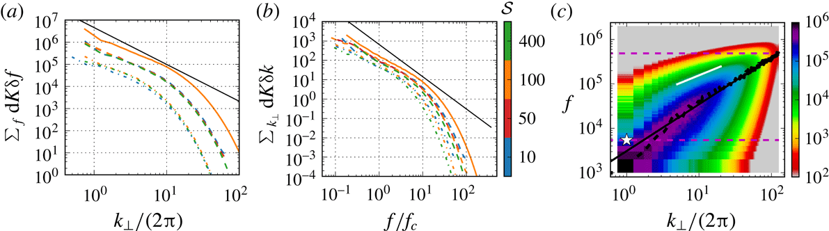
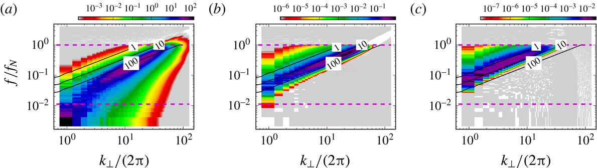
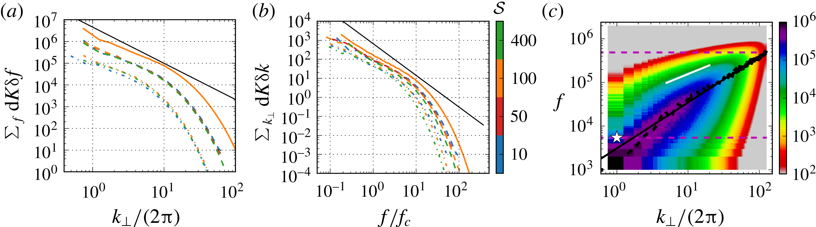
The theory described in § 3 assumes that the spatial correlations of the turbulent convection follow the standard Kolmogorov prediction for homogeneous and isotropic turbulence. Figure 2(a) shows that the frequency-integrated kinetic energy spectrum $\sum _{f}\text{d}K\unicode[STIX]{x1D6FF}f$ indeed has a slope relatively close to $k_{\bot }^{-5/3}$ for all simulations, thus validating the use of the Kolmogorov hypothesis. The theory also requires prescription of the temporal correlations of the turbulence fluctuations. Here, the theory uses the eddy turnover time as the relevant time scale, which is known as the straining hypothesis. However, one could argue that the temporal correlations of small-scale turbulent features seen at a fixed point in space are affected by the advection by large-scale motions, and that the sweeping hypothesis should be considered instead (Tennekes Reference Tennekes1975; Chen & Kraichnan Reference Chen and Kraichnan1989). The wavenumber-integrated kinetic energy spectrum in figure 2(b) shows a frequency scaling somewhat weaker than $f^{-5/3}$ , which is the typical scaling for turbulent flows in Eulerian frames with sweeping (Chevillard et al. Reference Chevillard, Roux, Lévêque, Mordant, Pinton and Arnéodo2005; Canet et al. Reference Canet, Rossetto, Wschebor and Balarac2017), in agreement with convection experiments (Sano, Wu & Libchaber Reference Sano, Wu and Libchaber1989). The straining mechanism would instead lead to a steeper $f^{-2}$ scaling, which is recovered when computing temporal correlations along Lagrangian trajectories in homogeneous turbulence (Chevillard et al. Reference Chevillard, Roux, Lévêque, Mordant, Pinton and Arnéodo2005) and in Rayleigh–Bénard convection (Liot et al. Reference Liot, Seychelles, Zonta, Chibbaro, Coudarchet, Gasteuil, Pinton, Salort and Chillà2016). Figure 2(c) shows $k_{\bot }\,f\text{d}K$ for simulation $C_{9}^{100}$ in $(k_{\bot },f)$ space, thus providing a more detailed picture of the turbulence statistics of the most turbulent simulation (similar results are obtained for other simulations). Again, it can be seen that the line of maximum $k_{\bot }\,f\text{d}K$ is reasonably well approximated by a power fit of the form $f\sim k_{\bot }^{a}$ (solid black line), with $a$ close to 1 for all simulations, suggesting strong sweeping effects. Isocontours at higher frequencies, however, have a milder slope $f\sim k_{\bot }^{b}$ with $b<1$ , possibly suggesting that the eddy dominant frequency does scale like ${\sim}k_{\bot }^{2/3}$ (solid white line) and that sweeping does not affect all eddies. We will show that there is a good agreement between DNS results and the theory based on the straining hypothesis despite the presence of a strong large-scale flow. It should be noted that the theory in § 3 changes with the choice of temporal correlations, as is already the case for other wave generation mechanisms by turbulence (for sound waves, see e.g. Zhou & Rubinstein Reference Zhou and Rubinstein1996; Favier, Godeferd & Cambon Reference Favier, Godeferd and Cambon2010).

Figure 2.

Integrated kinetic energy at $z=0.7$ as a function of (a) $k_{\bot }$ and (b) $f$ . Solid, dash–dash and dash–dot lines correspond to $Ra=4\times 10^{7},2\times 10^{8}$ and $10^{9}$ and different colours correspond to different stiffnesses. Black solid lines are power laws with slope $-5/3$ . (c) Kinetic energy spectrum $k_{\bot }\,f\text{d}K$ at $z=0.7$ for $C_{9}^{100}$ . The white star shows the wavenumber–frequency pair $(\ell _{c}^{-1},f_{c})$ of the large-scale circulation that allows a good agreement of the DNS with the theory. The pair $(\ell _{c}^{-1},f_{c})$ is not unreasonably far from the line $f(k_{\bot })$ of maximum energy, which is shown by the black dash–dash line (with the black solid line showing the linear fit). Dashed purple lines show $f_{c},f_{N}$ . The solid white line shows slope $+2/3$ .

4.2 Integrated wave energy flux

In this section we compare the total energy flux $F(z)$ obtained in DNS with the theoretical prediction $F^{th}(z)$ (cf. (3.8)), and we infer the free parameters of the theory ${\mathcal{A}}$ and $f_{c}$ from a best fit. The theoretical total flux $F^{th}$ has a steep scaling with the buoyancy frequency $f_{N}$ , the interface height $z_{i}$ and the turbulence parameters $\ell _{c}$ , $f_{c}$ and $u_{c}$ . While $f_{N}$ and $z_{i}$ are relatively well-constrained, the turbulence parameters are challenging to estimate from DNS of turbulent convection, making $F^{th}$ potentially highly sensitive to the definitions used. A slight variation of $f_{c}$ by a factor of 2, due to a change of definition, can lead to a change of $F^{th}$ by a factor of approximately 200 at all heights. Here, instead of estimating the values of the turbulence parameters using ad hoc definitions, we use a best-fit approach. For simplicity, we assume that $\ell _{c}=1$ in all cases and thus take $u_{c}=f_{c}$ . This leaves $f_{c}$ as the only free parameter in the theory, besides ${\mathcal{A}}$ , which is assumed to be the same for all simulations. A posteriori, we check that the best-fit $f_{c}$ is not too different from the r.m.s. velocity $u_{rms}=\sqrt{2K}$ at $z=0.7$ in the convection zone (cf. (2.5) and note that $u_{rms}$ is relatively depth-invariant in the convective bulk).

We obtain $f_{c}$ for each simulation case by requiring that the asymptotic prediction (3.8) equals the total flux in DNS at some height $z^{\ast }$ in the wave region, i.e.

(4.1) $$\begin{eqnarray}f_{c}^{21/2}=\frac{F(z^{\ast })}{{\mathcal{A}}}f_{N}^{47/8}\frac{28(8\unicode[STIX]{x03C0}^{2})^{13/8}}{5\unicode[STIX]{x1D6E4}\left(5/8\right)}\left(z^{\ast }-z_{i}\right)^{13/8}.\end{eqnarray}$$

This definition of $f_{c}$ may appear degenerate since $f_{c}$ can take different values depending on ${\mathcal{A}}$ or $z^{\ast }$ . However, as discussed below (cf. also figure 3 a), once ${\mathcal{A}}$ is chosen, $f_{c}$ does not depend on $z^{\ast }$ provided that $z^{\ast }$ is sufficiently far from the interface $z_{i}=1$ (i.e. $z^{\ast }>1.1$ ). With ${\mathcal{A}}\sim O(10)$ , we find for all simulations that $f_{c}$ is almost equal to $u_{rms}$ (to within a factor of two), which can be considered as a reference value for the turnover time of the largest-scale eddies (Lecoanet et al. Reference Lecoanet, Le Bars, Burns, Vasil, Brown, Quataert and Oishi2015). From now on we set the multiplicative constant arbitrarily to ${\mathcal{A}}=30$ . Other values could be chosen, but do not lead to significant changes as long as $f_{c}$ is relatively close to $u_{rms}$ .

Figure 3.

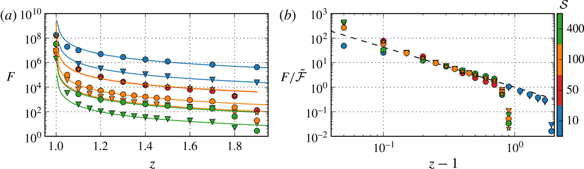
(a) Total flux in the wave region in DNS (triangles, circles, stars show results for $Ra=4\times 10^{7},2\times 10^{8},10^{9}$ ) along with the prediction $F^{th}$ ((3.8); solid lines) using the best-fit values for ${\mathcal{A}}$ and $f_{c}$ reported in table 1. (b) The normalized flux $F/\tilde{{\mathcal{F}}}$ is close to the prediction $F^{th}/\tilde{{\mathcal{F}}}\approx (z-1)^{-13/8}$ (dashed line) for $(z-1)\in [0.1,0.8]$ .

We compare DNS results for $F(z)$ (symbols) with the theoretical prediction $F^{th}(z)$ (solid lines) in figure 3(a) for all simulation cases, using the parameter values listed in table 1 (with ${\mathcal{A}}=30$ ). The total wave flux decreases with $z$ in all cases and, as expected, is larger for higher $Ra$ (for fixed ${\mathcal{S}}$ ) and lower ${\mathcal{S}}$ (for fixed $Ra$ ) (Couston et al. Reference Couston, Lecoanet, Favier and Le Bars2017). With $f_{c}$ obtained from a best fit at just one particular height, we find an excellent agreement between DNS and the theoretical prediction in all of the bulk of the wave region ( $z\in [1.1,1.8]$ ) for all simulations, which demonstrates that $f_{c}$ would be similar for any $z^{\ast }\in [1.1,1.8]$ . The $(z-1)^{-13/8}$ scaling predicted by the asymptotic solution is well verified in figure 3(b), which shows the normalized wave flux $F/\tilde{{\mathcal{F}}}$ (cf. (3.8)). All DNS results collapse on the asymptotic solution $(z-1)^{-13/8}$ shown by the dashed line for $(z-1)\in [0.1,0.8]$ , demonstrating that the theoretical flux spectrum integrated over the full range of waves excited compares well with the total flux in DNS.

4.3 Wave energy flux spectrum

We now investigate in details the scalings of the wave flux spectrum $k_{\bot }\,f\text{d}F$ in DNS with $k_{\bot }$ and $f$ , and discuss how they compare with the theoretical prediction ${\sim}k_{\bot }^{4}f^{-13/2}$ . We first show in figure 4(a–c) the overall wave flux spectrum $k_{\bot }\,f\text{d}F$ in $(k_{\bot },f)$ space at heights $z=1,1.1,1.5$ for simulation $C_{9}^{100}$ , which is the most turbulent case. The wave flux at $z=1$ can be difficult to interpret because it contains traces from both all types of waves and overshooting plumes, with one or the other type dominating depending on whether the convection zone extends slightly above or slightly below $z=1$ . At $z=1.1,1.5$ , however, we are clearly in the propagating wave region and the spectrum has all of the features predicted by the theory: in the high-frequency, low-wavenumber range (top left corner), the wave flux spectrum decreases rapidly with frequency and increases with wavenumber up to a cutoff wavenumber. The line of maximum wave flux spectrum overlaps with an isocontour of the decay rate $2\unicode[STIX]{x1D6FE}$ (cf. solid black lines and (3.6)), and that isocontour is closer to the top left corner as $z$ increases because this corner corresponds to waves which are the least damped. The wave flux spectrum falls off quickly at frequencies $f>f_{N}$ (top dashed line), which is the maximum frequency for propagating waves. Note that while upward-going waves require $\text{d}F>0$ , few $(f,k_{\bot })$ modes can be seen to have azimuthally averaged $\text{d}F\leqslant 0$ in figures 4 (shown by white bins). However, they have negligible $|\text{d}F|$ compared to positive $\text{d}F$ ’s, which is why we restrict the colour map to $\text{d}F>0$ only.

Figure 4.

Wave flux spectrum $k_{\bot }\,f\text{d}F$ in DNS for case $C_{9}^{100}$ at (a) $z=1.0$ , (b) 1.1, (c) 1.5. The colour scale is shifted to lower values from (a) to (c) because the wave flux decreases with height. Solid black lines show isocontours of the decay rate $2\unicode[STIX]{x1D6FE}$ . Dashed purple lines show $f_{c},f_{N}$ . White bins indicate $k_{\bot }\,f\text{d}F$ values that are negative.

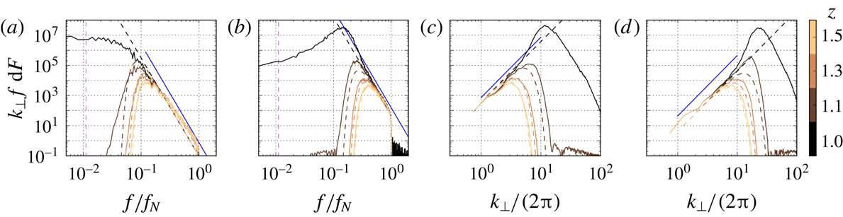
The wave flux spectrum is shown as a function of $f$ for fixed wavenumber in figure 5(a,b), and as a function of $k_{\bot }$ for fixed frequency in figure 5(c,d), providing a quantitative comparison of DNS results (solid lines) with the theory (dashed lines) for $C_{9}^{100}$ . The decrease of the wave flux spectrum in DNS with $f$ is steep and close to the predicted $f^{-13/2}$ scaling (shown by the blue solid line). The increase of the wave flux spectrum with $k_{\bot }$ closely follows the scaling $k_{\bot }^{4}$ , also predicted by the theory (shown by the blue solid line). Again, in figure 5(a,b) (respectively (c,d)) we note that the maximum flux moves towards higher frequencies (respectively lower wavenumbers) at higher $z$ as a result of damping. We have checked that similar trends in frequency space and wavenumber space are obtained for other fixed low wavenumbers (within the inertial subrange) and fixed high frequencies ( $f\gg u_{rms}$ ), suggesting an overall good agreement between DNS and theory for $C_{9}^{100}$ .

Figure 5.

Wave flux spectrum $k_{\bot }\,f\text{d}F$ for fixed $k_{\bot }/(2\unicode[STIX]{x03C0})=1.7,8.2$ (a,b) and fixed $f/f_{N}=0.2,0.4$ (c,d) for case $C_{9}^{100}$ . Lighter colours show results at higher heights. Solid lines show DNS results and dashed lines show theoretical results using the convection parameters listed in table 1. The blue lines show the theoretical scalings. The vertical dashed purple lines in (a,b) show $f_{c}/f_{N}$ .

Figure 6.

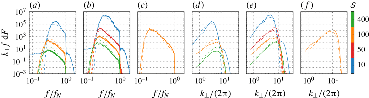
Wave flux spectrum $k_{\bot }\,f\text{d}F$ at $z=1.3$ for fixed $k_{\bot }/(2\unicode[STIX]{x03C0})=3.7$ (a–c) and fixed $f/f_{N}=0.4$ (d–f) with $Ra=4\times 10^{7},2\times 10^{8},10^{9}$ increasing from (a) to (c) and from (d) to (f). Different colours correspond to different stiffnesses ${\mathcal{S}}$ . Solid lines show DNS results and dashed lines show theoretical results using the convection parameters in table 1.

We now demonstrate that a good agreement is obtained between DNS and the theory not only for $C_{9}^{100}$ but for all simulations listed in table 1. In figure 6(a–c), we show the wave flux spectrum at $z=1.3$ as a function of $f$ for $k_{\bot }=3.7$ with $Ra=4\times 10^{7},2\times 10^{8},10^{9}$ , respectively. Clearly, the DNS results (solid lines) overlap well with the theoretical predictions (dashed lines) obtained after estimating the convective frequency $f_{c}$ from a best-fit approach (cf. § 4.2 and listed values in table 1). A good agreement is similarly obtained for the wave flux spectrum at $z=1.3$ as a function of $k_{\bot }$ and for $f/f_{N}=0.4$ between DNS and the theory (cf. figure 6 d–f).

5 Concluding remarks

We have shown that the scaling of the energy flux spectrum of internal waves generated by turbulent convection in DNS follows the $k_{\bot }^{4}\,f^{-13/2}$ prediction in the high- ${\mathcal{S}}$ regime (Lecoanet & Quataert Reference Lecoanet and Quataert2013), and consistently, the total flux decreases as $(z-1)^{-13/8}$ for all simulations presented. As discussed in the previous section, we can match the flux predicted by the theory to the DNS if we multiply the analytical prediction by a universal constant ${\mathcal{A}}$ and use a best fit for $f_{c}$ . It is unsurprising that the theory needs be rescaled since numerical factors have been dropped off along the derivation, and it is equally unsurprising that the best-fit $f_{c}$ equals a few times the reference frequency based on the r.m.s. velocity $u_{rms}$ . It is worth pointing out, however, that there are some variations of $f_{c}/u_{rms}$ across cases, which may mask some effects not included in the theory. Future work should explore the sweeping hypothesis, and include longer integration times with additional simulations or laboratory experiments in the high-turbulence, high- ${\mathcal{S}}$ regime.

It is remarkable that there is such a good agreement between the DNS and an approximate-at-best theory based on second-order statistics of turbulent motions. The theory, as simple as it is, may prove useful in assessing the detectability of internal waves in geophysical and astrophysical fluids such as stars and in estimating wave-driven changes of large-scale fluids from the energy in turbulent sources.