
1. Introduction
Continental shelf waves (CSWs) account for much of the low-frequency energy measured along coastlines. Since their discovery (Robinson Reference Robinson1964) there has been considerable discussion about continental shelves that account for depth changes only away from the coast while the depth remains unchanged along the coast. Huthnance (Reference Huthnance1975) has shown that for such a shelf superinertial waves exist, which include edge waves and Poincaré waves, as well as subinertial waves, which include CSWs and a Kelvin wave. If the ratio of the derivative of the depth function to the depth function is bounded everywhere, then the group velocity,  $c_{g}$, of CSWs is oppositely signed for long and short waves so that long waves travel with shallow water to the right and short waves with shallow water to the left. This implies that for such depth profiles, there is an intermediate wavenumber where CSWs have a maximum frequency for propagation, i.e. a cutoff frequency, and disturbances whose frequency exceeds the cutoff frequency are evanescent. Historically these CSWs were termed ‘trapped’, as they are trapped against the coast, although they propagate along the coast.
Continental shelf profiles, however, may vary alongshore. Grimshaw (Reference Grimshaw1977) and Huthnance (Reference Huthnance1987) discuss slow changes in the offshore wave profile and the propagation speed of CSWs as a shelf varies slowly in the alongshore direction. This implies that the  $c_{g}$ of any particular mode, at a fixed frequency, can vary in the alongstream direction and thus can vanish at more than point. It is shown in Kaoullas & Johnson (Reference Kaoullas and Johnson2012) and Johnson & Kaoullas (Reference Johnson and Kaoullas2011), that in the rigid-lid limit sufficiently large alongshore depth changes can lead to a local increase or a decrease in the cutoff frequency for propagation of CSWs. In particular, changes in the distance of the shelf break from the coastline or the slope of the shelf can be sufficient to create a localised region where CSWs can propagate at a higher frequency compared with the far field further along the coast. This leads to the possibility of CSWs becoming trapped both away from the coast and also away from the localised alongshore depth region so no energy at this higher frequency propagates along the coast. These modes consist of a slowly varying long wave, propagating with shallow water to the right until the
 $c_{g}$ vanishes, at which point it reflects as a short wave propagating with deep water to its right, until its
 $c_{g}$ vanishes and it is reflected back as long wave. These modes are then confined along the coast and will be referred to below as trapped CSWs (tCSWs). Examples of shelf-coastline geometries that admit tCSWs (i.e. submerged ridges and bays) were shown with asymptotic and numerical methods in Kaoullas & Johnson (Reference Kaoullas and Johnson2012). Changes in coastline curvature (while isobaths remained parallel to the coast) have also been shown by Johnson, Levitin & Parnovski (Reference Johnson, Levitin and Parnovski2006) rigorously to admit tCSWs under (weak) geometric assumptions provided the shelf bends towards the coast, i.e. shallow water. Explicit examples of such curved coastline geometries where given in Postnova & Craster (Reference Postnova and Craster2008), Kaoullas & Johnson (Reference Kaoullas and Johnson2010b) and Kaoullas & Johnson (Reference Kaoullas and Johnson2012).
Trapped modes exist in other physical settings. Asymptotic and numerical results have been obtained for problems concerning waveguides in elasticity (Gridin, Craster & Adamou Reference Gridin, Craster and Adamou2005; Kaplunov, Rogerson & Tovstik Reference Kaplunov, Rogerson and Tovstik2005; Postnova & Craster Reference Postnova and Craster2008) and existence proofs given for quantum (Exner & Seba Reference Exner and Seba1989; Duclos & Exner Reference Duclos and Exner1995; Dittrich & Kriz Reference Dittrich and Kriz2002; Krejčiřík & Kříž Reference Krejčiřík and Kříž2005) and acoustic problems (Evans, Levitin & Vassiliev Reference Evans, Levitin and Vassiliev1994; Davies & Parnovski Reference Davies and Parnovski1998; Aslanyan, Parnovski & Vassiliev Reference Aslanyan, Parnovski and Vassiliev2000). The acoustic waveguide problem (with Neumann boundary conditions) corresponds directly to non-rotating water waves in an infinitely long channel of constant depth. These problems are of particular interest as the essential spectrum of the frequency is bounded at zero, i.e.  $[0,\infty )$, but the addition of symmetric, fully submerged obstacles (see e.g. Evans et al. Reference Evans, Levitin and Vassiliev1994; Linton & McIver Reference Linton and McIver1998, Reference Linton and McIver2007) leads to a discrete eigenvalue lying inside the essential spectrum giving an embedded trapped mode.
Approximating the full shelf wave problem by taking the water surface to be rigid allows a stream function formulation of the problem (Buchwald & Adams Reference Buchwald and Adams1968; LeBlond & Mysak Reference LeBlond and Mysak1978) where the Kelvin and Poincaré waves are absent and the continuous frequency spectrum has an upper bound, i.e. the cutoff frequency (Johnson et al. Reference Johnson, Levitin and Parnovski2006). The eigenvalue problem for the frequency  $\omega$ is linear and the boundary condition (b.c.) at the coast is Dirichlet. The rigid-lid approximation is valid for where the external Rossby radius of deformation is large compared with the shelf width and applies to most midlatitude shelves. The approximation can be poor on some shelves even in midlatitude (see e.g. Schulz, Mied & Snow Reference Schulz, Mied and Snow2012). Relaxing the rigid-lid approximation introduces a Kelvin wave, present at all frequencies, and super-inertial Poincaré waves. This means that the continuous spectrum of the wave operator is no longer bounded so either energy leaks into the Kelvin wave and no tCSWs exist or, if tCSWs exist, they are embedded in the continuous spectrum. These lead to a distinctly different and more challenging analytical problem.
It is the purpose of this work to show that tCSWs can indeed exist for a non-rectilinear shelf geometry even in the presence of a free surface. Section 2 formulates the problem and § 3 considers rectilinear shelves to establish the non-rectilinear shelf geometry that can lead to trapping. By employing a simple but efficient numerical method, it is shown that changing the slope across the shelf (i.e. a submerged ridge) raises the cutoff frequency for CSWs and thus can lead to trapping. The asymptotic method is presented in § 4 where the shelf is modelled as a waveguide, by approximating the shelf–ocean boundary as a rigid wall. The topography chosen varies slowly along the shelf, so the scale of the alongshelf variations of the isobaths is large compared with the shelf's width. A regular asymptotic expansion leads to a hierarchy of equations, where the problem is reduced to finding the solutions of a second-order differential equation in the alongshelf direction. The rigid-lid case is also summarised since it follows immediately from our analysis. Subsequently it is shown that a submerged ridge can support trapped modes while a submerged valley does not. The accuracy of the asymptotic method is demonstrated by employing a highly accurate pseudospectral method that solves the full equation and demonstrates that the results of both methods are in close agreement. In § 5 we consider a non-rectilinear shelf that abuts to open ocean, thus eliminating the approximate b.c. at the shelf–ocean boundary. The trapping of CSWs is shown numerically, and it also shown that the frequency of trapping, when considering an open-ocean geometry, is bounded below by the respective frequency of a trapped mode when the approximate b.c. at the shelf–ocean boundary is considered. Finally, a brief discussion of our results is given in § 6.
2. Formulation of the problem
The linearised shallow water equations can be written as
 \begin{gather} u_{t}-fv =-g\eta_{x}, \end{gather}
 \begin{gather}v_{t}+fu =-g\eta_{y}, \end{gather}
 \begin{gather}\eta_{t}+(u H)_{x}+(v H)_{y}=0, \end{gather}
where  $f$ is the Coriolis parameter (assumed constant),
 $g$ is the gravitational acceleration,
 $u(x,y,t)$ and
 $v(x,y,t)$ are the components of the horizontal velocity,
 $\eta (x,y,t)$ is the free-surface displacement and
 $H(x,y)$ is the undisturbed fluid depth. Equations (2.1)–(2.3) can be rearranged to give an equation for
 $\eta$ alone (see e.g. LeBlond & Mysak Reference LeBlond and Mysak1978),
 \begin{equation} (\partial_{tt}+f^2)\eta_{t}-g\boldsymbol{\nabla}\boldsymbol{\cdot}(H\boldsymbol{\nabla}\eta_{t}) +gf\boldsymbol{\hat{z}}\boldsymbol{\cdot}(\boldsymbol{\nabla}\eta \times\boldsymbol{\nabla} H)=0. \end{equation}
Taking the coastline as impermeable gives the b.c.
 \begin{equation} \eta_{yt}-f\eta_{x}=0,\quad y=0, \end{equation}
and the full problem, solved numerically in § 5, has the open-ocean b.c.
 \begin{equation} \eta\rightarrow 0,\quad y\rightarrow \infty. \end{equation}
This is approximated in § 4 by taking the shelf–ocean boundary to be impermeable, so
 \begin{equation} \eta_{yt}-f\eta_{x}=0,\quad y=1. \end{equation}
In the rigid-lid case, using the stream function formulation, Johnson (Reference Johnson1989) has shown that demanding that the normal component of the velocity vanishes at the shelf–ocean boundary gives a lower bound to the frequency of trapping, which is accurate in the short-wave limit. Even though no analogous result exists for the free-surface formulation, the approximate b.c. (2.7) gives a clearer problem to deal with for the asymptotic method, allowing explicit solutions to be derived for simple topographies in the rigid-lid case. Note that, this b.c. admits a Kelvin wave (also present at all frequencies) propagating along the outer wall in the opposite direction of the rest of the waves considered here, and thus does not interact with them.
For periodic solutions of the form
 \begin{equation} \eta=\textrm{Re}\{\varPhi(x,y)\exp(-\textrm{i}\omega ft)\}, \end{equation}
(2.4) reduces to
 \begin{equation} \omega\boldsymbol{\nabla}\boldsymbol{\cdot}(H\boldsymbol{\nabla}\varPhi)-\textrm{i}\hat{z}\boldsymbol{\cdot} (\boldsymbol{\nabla}\varPhi \times\boldsymbol{\nabla} H)+[(\omega^{3}-\omega)/R^2]\varPhi=0, \end{equation}
where  $\omega$ is the non-dimensional frequency,
 $R=\sqrt {gH_{m}}/fL$ is the non-dimensional parameter which gives the ratio of the Rossby radius of deformation to the shelf width L and
 $H_{m}$ is the dimensional depth at the ocean. All depths are scaled to
 $H_{m}$. The depth profile
 $H$ has been scaled to equal 1 at the deepest end and is constant in the ocean region
 $y>1$. Equation (2.9) is a cubic eigenvalue problem for the eigenvalue
 $\omega$ which also appears in the b.c.s (2.5) and (2.7). For low frequency modes where
 $\omega \ll 1,$ the term
 $\omega ^{3}$ can be neglected to give a linear eigenvalue problem (Rhines Reference Rhines1969). This also removes the Poincaré waves from the problem, however, this reduction is not necessary in the methods presented here.
3. Rectilinear shelf geometries
For any mode to become trapped, the geometry of the shelf must change along the shelf in such a way that CSWs can propagate at a higher frequency (locally) compared with the far field. For a rectilinear shelf, i.e. of the form  $H\equiv H(y)$, the spectrum of the operator in (2.9) subject to the b.c.s (2.5) and (2.7) or (2.6a,b) is purely continuous and has no trapped modes (Huthnance Reference Huthnance1975). However, in order to understand the nature of the spectrum of operator (2.9), with respect to shelf geometry changes, it is thus convenient to consider initially rectilinear shelves. Introducing
 $\varPhi =Y(y)\exp (\textrm {i} k x)$, where
 $k$ is the
 $x$-wavenumber, gives from (2.9) and (2.5)–(2.6a,b), for the channel model with rigid walls,
 \begin{gather} (HY')'+[kH'/\omega-k^{2}H+(\omega^{2}-1)/R^2]Y=0, \end{gather}
 \begin{gather}\omega Y'+kY=0,\quad y=0, \end{gather}
 \begin{gather}\omega Y'+kY=0,\quad y=1. \end{gather}
For the full model the shelf-ocean b.c (3.3) is replaced by the open-ocean condition
 \begin{equation} Y \rightarrow 0,\quad y\rightarrow \infty. \end{equation}
This one-dimensional problem can be easily solved with a highly accurate spectral, Chebyshev discretisation similarly to Kaoullas & Johnson (Reference Kaoullas and Johnson2010a). Appendix A gives the details. The open-ocean b.c. can be replaced with a nonlinear b.c. at the shelf–ocean boundary, however, for simplicity we will use a smooth topography function and extend the flat ocean sufficiently for offshore modes to decay. It is shown in Kaoullas & Johnson (Reference Kaoullas and Johnson2012), that for the rigid-lid case, locally changing the shelf slope or the distance of the shelf break from the coast can lead to trapped CSWs. Thus for the free-surface case consider the (rather more general) depth profile
 \begin{equation} H(\!y)=H_{0}+(1-H_{0})\{1+\tanh[(y-c)/s]\}/2, \end{equation}
where,  $c$ is the distance of the shelf break from the coast,
 $s$ is the slope of the shelf and
 $H_{0}$ the depth at the coast (for sufficiently large
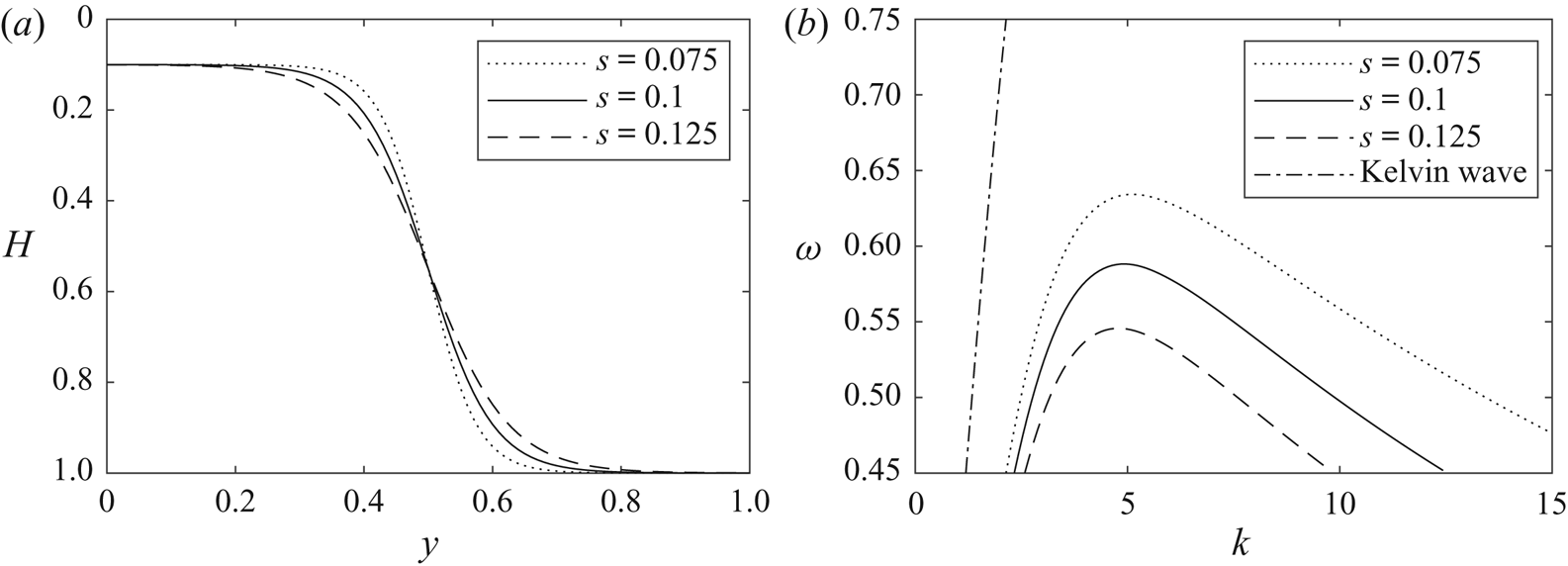
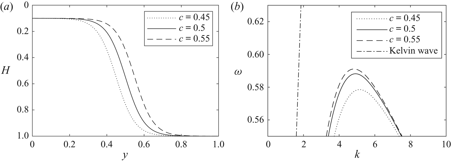
 $c/s$). Figure 1 shows (for the open-ocean model) that if the slope of the shelf increases, so too does the frequency at which waves can propagate. Similarly, as can be seen in figure 2, increasing the distance of the shelf break from the coast results in higher frequency of propagation. Trapping is thus possible although not proven. The coastal Kelvin wave is also present at all frequencies (almost unaffected by the change in shelf slope), implying that any tCSWs are embedded in the continuous spectrum. The same result is obtained for a channel with solid wall geometry (omitted here).
(a) Depth profiles and (b) dispersion curves of the first propagating mode and the Kelvin mode for various shelf slopes for the profile (3.5). Here,  $c=0.5$,
 $H_0=0.1$ and
 $R=1$.

(a) Depth profiles and (b) dispersion curves of the first propagating mode and the Kelvin mode for various shelf breaks for the profile (3.5). Here,  $s=0.1$,
 $H_0=0.1$ and
 $R=1$.

4. Asymptotic method
4.1. Slowly and slightly varying shelf geometry
The geometry here is the straight channel  $0\leq y \leq 1,$
 $-\infty \leq x \leq \infty$. Consider a non-rectilinear shelf such that, parallel to the channel the shelf depth changes only slowly and by a small amount with distance along the shelf, i.e.
 $H(\epsilon x, y) = H(\xi , y)$, where
 $\epsilon$ is a small dimensionless parameter representing the ratio of the shelf width to the scale of the longitudinal variation in offshore depth profile. It is possible to avoid the slightly varying approximation using the WKB method and solve the one-dimensional eigenvalue, cross-stream problem, at each station along the shelf, similarly to Rodney & Johnson (Reference Rodney and Johnson2015) and Rocha et al. (Reference Rocha, Bossy, Llewellyn Smith and Young2020) numerically, however, the slight variation employed here allows the alongstream structure to be obtained analytically. In the new coordinates
 $(\xi , y)$ the governing equation (2.9) and b.c.s (2.5) and (2.7) become
 \begin{gather} \omega[H(\epsilon^{2}\varPhi_{\xi\xi}+\varPhi_{yy})+(\epsilon^{2}H_{\xi}\varPhi_{\xi}+H_{y}\varPhi_{y})] +\epsilon\textrm{i}(H_{\xi}\varPhi_{y}-H_{y}\varPhi_{\xi})+[(\omega^{3}-\omega)/R^2]\varPhi=0, \end{gather}
 \begin{gather} \textrm{i}\omega\varPhi_{y}+\epsilon\varPhi_{\xi}=0,\quad y=0, \end{gather}
 \begin{gather}\textrm{i}\omega\varPhi_{y}+\epsilon\varPhi_{\xi}=0,\quad y=1. \end{gather}
We now make the following regular asymptotic expansion:
 \begin{gather} \varPhi\sim \exp( \textrm{i} \mu\xi/\epsilon)\varPsi,\quad \varPsi=f_{0}(\xi)\varPsi^{c}(y)+\epsilon \varPsi_{1}(\xi,y)+\epsilon^{2} \varPsi_{2}(\xi,y)+\cdots, \end{gather}
 \begin{gather}\omega=\omega_{0}+\epsilon \omega_{1}+\epsilon^{2}\omega_{2}+\cdots, \end{gather}
where  $\omega _{0}$ is the cutoff frequency,
 $\varPsi ^{c}(y)$ the corresponding solution to the one-dimensional problem,
 $f_{0}(\xi )$ is the alongstream solution (i.e. the envelope) and
 $\mu$ is the
 $x$-wavenumber at the cutoff frequency, i.e. the maximum frequency of propagation as a function of the alongshore wavenumber. Expansion (4.5) differs from those in Postnova & Craster (Reference Postnova and Craster2008) and Kaoullas & Johnson (Reference Kaoullas and Johnson2012), which are expansions in powers of the reciprocal of the frequency.
The strategy here is to obtain a hierarchy of equations where, to leading order, the cross-stream structure of the modes for a rectilinear shelf are determined, and to second order, the mechanisms of trapping are given by a second-order ordinary differential equation for  $f_{0}(\xi )$ (see below). Readers who want to skip the mathematical details can proceed to §§ 4.3 and 5. Substituting the first of (4.4a,b) into (4.1)–(4.3) we get
 \begin{align} & \epsilon^{2}\varPsi_{\xi\xi}+\varPsi_{yy}+\left(\epsilon^{2}\frac{H_{\xi}}{H}-\epsilon \frac{\textrm{i}}{\omega}\frac{H_{y}}{H}+ \epsilon 2\textrm{i}\mu\right)\varPsi_{\xi}+ \left(\frac{H_{y}}{H}+ \epsilon\frac{\textrm{i}}{\omega}\frac{H_{\xi}}{H}\right)\varPsi_{y} \nonumber\\ &\quad +\left(\epsilon \textrm{i}\mu \frac{H_{\xi}}{H}+ \frac{\mu}{\omega}\frac{H_{y}}{H}-\mu^{2}+ \frac{\omega^{2}-1}{HR^2}\right)\varPsi=0, \end{align}
 \begin{equation} \textrm{i}\omega\varPsi_{y}+\textrm{i} \mu\varPsi+\epsilon\varPsi_{\xi}=0,\quad y=0,1.\end{equation}
The expansion simplifies for the exponential depth profile
 \begin{equation} H(x,y)=\exp\left(2b p(\xi,y)\right), \quad y\in[0,1] , \end{equation}
where
 \begin{gather} p(\xi,y)=(y-1+y(1-y)\alpha\epsilon^{2}\gamma(\xi)), \end{gather}
 \begin{gather}p_{y}=1+(1-2y)\alpha\epsilon^{2}\gamma(\xi),\quad p_{\xi} =y(1-y)\alpha\epsilon^{2}\gamma_{\xi}(\xi), \end{gather}
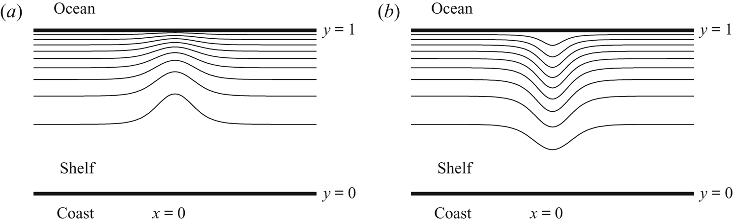
corresponding to a submerged ridge for  $\alpha <0$ (figure 3a) and a submerged valley for
 $\alpha >0$ (figure 3b). For convenience the amplitude of the change in depth profile along
 $\xi$, in (4.8), has been scaled to
 $\epsilon ^{2}$ (while the slow variation is of order
 $\epsilon$) so that the variation in
 $\xi$ would only appear to order
 $\epsilon ^{2}$ and thus the geometry now is more slight than slow. Then (4.6) becomes
 \begin{align} & \epsilon^{2}\varPsi_{\xi\xi}+\varPsi_{yy}+(\epsilon^{2}2bp_{\xi}+ \epsilon 2\textrm{i}(\mu-bp_{y}/\omega))\varPsi_{\xi}+2b(p_{y}+ \epsilon \textrm{i} p_{\xi}/\omega)\varPsi_{y}\nonumber\\ &\quad +(\epsilon 2b\textrm{i}\mu p_{\xi}+2b\mu p_{y}/\omega-\mu^{2}+ (\omega^{2}-1)/(HR^2))\varPsi=0. \end{align}
Now
 \begin{equation} \omega^{3}-\omega=\omega_{0}^{3}-\omega_{0}+\epsilon\omega_{1}(3\omega_{0}^{2}-1)+ \epsilon^{2}(3\omega_{0}\omega_{1}^{2}+ 3\omega_{0}^{2}\omega_{2}-\omega_{2} ) +O(\epsilon^{3}), \end{equation}
and the Taylor series expansion of the reciprocal of the depth profile is
 \begin{equation} H^{-1}(\xi,y)=\textrm{e}^{{2b(1-y)}}(1-\epsilon^{2}2by(1-y)\alpha \gamma(\xi)+O(\epsilon^{4})), \end{equation}
giving the leading-order equation
 \begin{gather} (h\varPsi^{c}_{y})_{y}+ [2b\mu/\omega_{0}-\mu^{2}+(\omega_{0}^{2}-1)/(hR^2)]h\varPsi^{c}=0, \end{gather}
 \begin{gather}\omega_{0}\varPsi^{c}_{y}+\mu\varPsi^{c}=0,\quad y=0,1, \end{gather}
where  $h(y)=\exp (2b(y-1))$. Equation (4.14) with b.c.s (4.15) is to be solved numerically using the numerical method introduced in Appendix A. Solutions are normalised by requiring
 \begin{equation} \int_{0}^{1}h\varPsi^{c2} \,\textrm{d} y=1. \end{equation}
Multiplying (4.14) by  $\varPsi ^{c}$, integrating over
 $y\in [0,1]$ and using (4.15) gives the dispersion relation,
 \begin{equation} -k_{0}[h\varPsi^{c 2}]^{1}_{0}-\omega_{0}\int_{0}^{1} h \varPsi^{c 2}_{y}\,\textrm{d} y +2bk_{0}-\omega_{0}k_{0}^{2}+ (\omega_{0}^{3}-\omega_{0})/R^2\int_{0}^{1}\varPsi^{c 2}\,\textrm{d} y =0, \end{equation}
on setting  $\mu =k_{0}$, the
 $x$-wavenumber at the cutoff frequency,
 $\omega _{0}$, of the rectilinear channel (
 $\epsilon =0$). Differentiating (4.17) with respect to
 $k_{0}$ and setting the group velocity to zero gives
 \begin{equation} 2b-\left[h\varPsi^{c 2}\right]^{1}_{0}=2k_{0}\omega_{0}=2\mu\omega_{0}. \end{equation}
Unlike the rigid-lid case (Kaoullas & Johnson Reference Kaoullas and Johnson2012; Rodney & Johnson Reference Rodney and Johnson2015), the bracketed term in (4.18) is non-zero; this proves crucial below. At the next order
 \begin{align} & (h\varPsi_{1_{y}})_{y}+ [2b\mu/\omega_{0}-\mu^{2}+(\omega_{0}^{2}-1)/(hR^2)]h\varPsi_{1} +2\omega_{1} (\omega_{0}/(h R^{2})\nonumber\\ &\quad -b\mu/\omega_{0}^{2})h f_{0}\varPsi^{c} +2\textrm{i}(\mu-b/\omega_{0})hf_{0_{\xi}}\varPsi^{c}=0, \end{align}
 \begin{equation} \textrm{i}\omega_{0}\varPsi_{1_{y}}+\textrm{i}\mu\varPsi_{1}+\textrm{i}\omega_{1}f_{0}\varPsi^{c}_{y}+f_{0_{\xi}}\varPsi^{c}=0,\quad y=0,1,\end{equation}
where  $f_{0}(\xi )$ is the alongstream structure of the solution (see (4.4a,b)) which needs to be determined. Multiplying (4.19) by
 $\varPsi ^{c}$ and integrating over
 $y\in [0,1]$ gives
 \begin{equation} \left[h\varPsi_{1_{y}}\varPsi^{c}-h\varPsi_{1}\varPsi_{y}^{c}\right]_{0}^{1}+ \frac{2\omega_{1}}{\omega_{0}}f_{0}\left(\frac{\omega_{0}^{2}}{ R^{2}} \int_{0}^{1}\varPsi^{c2} \,\textrm{d} y-\frac{b\mu}{\omega_{0}}\right)+ 2\textrm{i}\left(\mu-\frac{b}{\omega_{0}}\right)f_{0_{\xi}}=0.\end{equation}
Using (4.18) and the b.c.s (4.15) and (4.20), equation simplifies (4.21) to
 \begin{equation} 2\omega_{1}f_{0}\left(\frac{\omega_{0}}{R^{2}}\int_{0}^{1}\varPsi^{c2}\,\textrm{d} y -\frac{\mu^{2}}{\omega_{0}}\right)=0. \end{equation}
For a non-trivial solution  $f_{0}$ is non-zero, so either
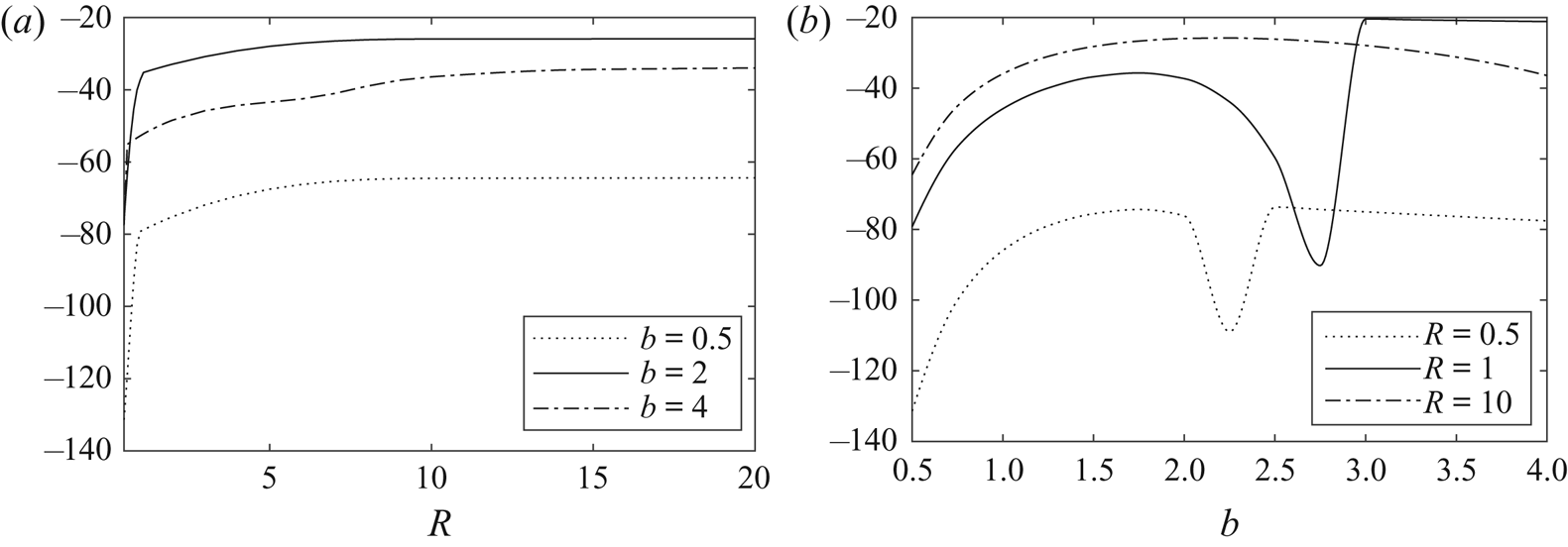
 $\omega _{1}=0$ or the bracketed term in (4.22) vanishes. As can be seen from figure 4, for all values of
 $b>0$ and
 $R> 0$, the term in the brackets is non-zero which forces
 $\omega _{1}=0$. It remains to determine
 $\varPsi _{1}$, from
 \begin{gather} \varPsi_{1_{yy}}+2b\varPsi_{1_{y}}+ [2b\mu/\omega_{0}-\mu^{2}+(\omega_{0}^{2}-1)/(hR^2)] \varPsi_{1} = -2\textrm{i}\left(\mu-b/\omega_{0}\right)f_{0_{\xi}}\varPsi^{c}, \end{gather}
 \begin{gather}\omega_{0}\varPsi_{1_{y}}+\mu\varPsi_{1}=\textrm{i} f_{0_{\xi}}\varPsi^{c},\quad y=0,1. \end{gather}
This is a non-homogeneous ordinary differential equation with solution
 \begin{equation} \varPsi_{1}=f_{1}(\xi)\varPsi^{c}+M(y)f_{0_{\xi}},\end{equation}
where  $M$ is to be determined. Substituting (4.25) into (4.23) and (4.24) we get an ordinary differential equation for
 $M$ as follows:
 \begin{gather} M_{yy}+2bM_{y}+[2b\mu/\omega_{0}-\mu^{2}+(\omega_{0}^{2}-1)/(hR^2)]M =-2\textrm{i}\left(\mu-b/\omega_{0}\right)\varPsi^{c}, \end{gather}
 \begin{gather}\omega_{0}M_{y}+\mu M=\textrm{i} \varPsi^{c},\quad y=0,1. \end{gather}
Since  $\omega _{0}$,
 $\mu$ and
 $\varPsi ^{c}$ have been determined, through (4.14), (4.15) and (4.18), equation (4.26) can be solved straightforwardly numerically as a non-homogeneous, linear system of equations. To double precision the resulting matrix is ill-conditioned, and thus required higher precision using the Advanpix (2019) multiprecision toolkit for Matlab. The order
 $\epsilon ^{2}$ equation is
 \begin{align} & (h\varPsi_{2_{y}})_{y}+[2b\mu/\omega_{0}-\mu^{2}+(\omega_{0}^{2}-1)/(hR^2)]h\varPsi_{2} +2\omega_{2} (\omega_{0}/(h R^{2})\nonumber\\ &\quad -b\mu/\omega_{0}^{2})h\varPsi^{c}f_{0}+hf_{0_{\xi\xi}}\varPsi^{c} + 2\textrm{i}(\mu-b/\omega_{0})h\varPsi_{1_{\xi}}+2b\alpha \gamma h [(1-2y)\nonumber\\ &\quad \times (\varPsi^{c}_{y}+(\mu/\omega_{0})\varPsi^{c})-y(1-y) (\omega_{0}^{2}-1)/(hR^{2})\varPsi^{c}]f_{0}=0, \end{align}
 \begin{equation} \textrm{i}\omega_{0}\varPsi_{2_{y}}+\textrm{i}\mu\varPsi_{2}+\textrm{i}\omega_{2}f_{0}\varPsi^{c}_{y}+\varPsi_{1_{\xi}}=0,\quad y=0,1.\end{equation}
Multiplying (4.28) by  $\varPsi ^{c}$ and integrating gives
 \begin{equation} I_{1}f_{0_{\xi\xi}}+V(\xi)f_{0}=\omega_{2}I_{2}f_{0}, \end{equation}
where
 \begin{align} V(\xi) &= \alpha 2b \gamma(\xi)\left(\int_{0}^{1} h(1-2y)(\varPsi^{c}\varPsi^{c}_{y}+(\mu/\omega_{0})\varPsi^{c2})\,\textrm{d} y \right. \nonumber\\ &\quad \left. -\frac{\omega_{0}^{2}-1}{R^{2}}\int_{0}^{1} y(1-y)\varPsi^{c2}\,\textrm{d} y \right), \end{align}
 \begin{gather} I_{1}=1+\frac{\textrm{i}}{\omega_{0}}\left[hM\varPsi^{c}\right]_{0}^{1}+2\textrm{i}\left(\mu-\frac{b}{\omega_{0}}\right) \int_{0}^{1} hM\varPsi^{c}\,\textrm{d} y, \end{gather}
 \begin{gather}I_{2}=\frac{2}{\omega_{0}}\left(\mu^{2}-\frac{\omega_{0}^{2}}{R^{2}}\int_{0}^{1}\varPsi^{c2}\,\textrm{d} y \right). \end{gather}
Equation (4.30) is a one-dimensional Schrödinger equation with  $V$ the associated potential and
 $\omega _{2}$ the eigenvalue. It can be determined numerically, similarly to figure 4 (not shown here), that
 $I_{1}>0$ and the term in the brackets in (4.31) is negative. For a trapped mode to exist, its frequency must lie above the cutoff frequency of the unperturbed channel and so from (4.5),
 $\omega _{2}$ is positive. Following Gridin et al. (Reference Gridin, Craster and Adamou2005), multiplying both sides of (4.30) by
 $f_{0}$ and integrating by parts on
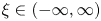 $\xi \in (-\infty ,\infty )$ gives
 \begin{equation} -I_{1}\int_{-\infty}^{\infty}(f_{0_{\xi}})^{2}\,\textrm{d}\xi+ \int_{-\infty}^{\infty}V(\xi)\left(f_{0}\right)^{2}\,\textrm{d}\xi= I_{2}\omega_{2} \int_{-\infty}^{\infty}\left(f_{0}\right)^{2}\,\textrm{d}\xi,\end{equation}
where we have used the requirement for trapped modes, that  $f_{0}$ vanishes at infinity. If the second integral in (4.34) is negative, i.e.
 $V<0$, the left-hand side of (4.34) becomes negative, forcing
 $\omega _{2}$ to be negative (since
 $I_{2}$ is positive from figure 4), thus no trapping is possible. Hence if
 $V$ is positive, trapped modes might exist (depending on the magnitude of
 $V$).
Isobaths (not drawn to scale) of (a) a submerged ridge ( $\alpha <0$) and (b) a submerged valley (
 $\alpha >0$).

The bracketed term in (4.22) computed numerically for (a)  $b$ fixed against various values of
 $R$ and (b)
 $R$ fixed against various values of
 $b$.

In the rigid-lid case, i.e.  $R\rightarrow \infty$, closed form solutions exist for the depth profile (4.8). The analysis is identical to § 4.1 and so we refer the reader to appendix B for the derivation of these solutions.
4.2. Analytical solution
Choosing 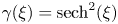 $\gamma (\xi )=\textrm {sech}^{2}(\xi )$, allows (4.30) to be solved analytically following Landau & Lifshitz (Reference Landau and Lifshitz1991) as
 \begin{equation} f_{0}(\xi)=\cosh^{m-s}(\xi)F\left(-m;2s+1-m;s+1-m;(1-\tanh{\xi})/2\right), \end{equation}
where
 \begin{equation} s=(\sqrt{1+4\alpha\beta}-1)/2,\quad \omega_{2}=(s-m)^{2}I_{1}/I_{2},\quad 0\leq m<s, \end{equation}
and  $F$ is the confluent hypergeometric function of degree m. Here
 $-m$ is a positive integer, and so
 $F$ is a polynomial of degree
 $m$ with
 $\beta$ given by
 \begin{align} \beta= \begin{cases} -2b & \mbox{rigid-lid}, \\ V/I_{1} & \mbox{full problem}, \end{cases} \end{align}
for  $V$ and
 $I_{1}$ given by (4.31) and (4.32), respectively. The condition that
 $s>m$ gives the lower bound on the parameter
 $\alpha$:
 \begin{equation} -\alpha>[(2m-1)^{2}-1]/4\beta.\end{equation}
For the first transverse mode  $(m=1)$ to become trapped, condition (4.38) requires simply that
 $\alpha <0$. Thus, provided there is a perturbation in depth leading to a submerged ridge, i.e.
 $\alpha <0$, the first alongshelf mode is trapped. The corresponding cross-shelf mode number is arbitrary, leading to a countably infinite set of trapped modes. For higher alongshore modes to get be trapped, a larger value of
 $|\alpha |$ is required, corresponding to a larger magnitude of the potential
 $V$ and hence to a larger amplitude in the depth perturbation.
4.3. Numerical method and results
The full equation (4.6) with b.c.s (4.7), can be written as
 \begin{align} & \omega^{4}/(HR^2)\varPsi+\omega^{2}(\varPsi_{xx}+\varPsi_{yy}+2b(p_{x}\varPsi_{x}+p_{y}\varPsi_{y})-1/(HR^2)\varPsi)\nonumber\\ &\quad +\omega 2b\textrm{i}([1-p_{y}]\varPsi_{x}+p_{x}\varPsi_{y}+bp_{x}\varPsi)+b^{2}(2 p_{y}-1)\varPsi=0, \end{align}
 \begin{equation} \omega^{2}\varPsi_{y}-\textrm{i}\omega\varPsi_{x}+b\varPsi=0,\quad y=0,1,\end{equation}
using the relation  $\mu =b/\omega$ to eliminate (most of) the phase from the fast carrier wave in the alongstream direction. This relation is exact for the rigid-lid problem (hence all of the phase is removed) and a good approximation for the full problem (compared with the analogue of (4.18)). This slight approximation for the full problem allows stable numerical computations and, with most of the rapid phase variation removed, requires much smaller matrices to accurately solve the eigenvalue problem. A highly accurate pseudospectral method was employed, with a Chebyshev grid discretisation in the cross-stream direction and a Hermite grid in the alongstream direction. When dealing with unbounded domains the accuracy of the solution is greatly improved with the appropriate choice of a scale factor (Tang Reference Tang1993; Weideman & Reddy Reference Weideman and Reddy2000; Shen & Wang Reference Shen and Wang2009) so that the largest collocation point lies where the solution is smaller than a desired value (see Kaoullas & Johnson (Reference Kaoullas and Johnson2012), for more details). Appendix C gives details on linearising this polynomial eigenvalue problem (4.39), for the eigenvalue
 $\omega$, to a generalised eigenvalue problem and imposing the b.c.s (4.40). The linearisation of any polynomial eigenvalue problem is not unique and the associated backwards error is an open topic of research (Tisseur Reference Tisseur2000). The choice here leads to reasonably conditioned matrices.
Let  $\omega _{m,n}$ denote the frequency of the
 $(m,n)$ tCSW, where
 $m$ is the alongshore mode number and
 $n$ the cross-shelf mode number so that
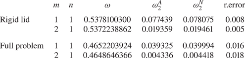
 $m=1$ corresponds to the fundamental mode. Table 1 shows the accuracy of the asymptotic method, when compared with the numerical solution of (4.6), for the rigid-lid and the full problem. In particular, the accuracy of
 $\omega _{2}$ which is the next order correction to the cutoff frequency of the asymptotic method (
 $\omega _{2}^{A}$), is assessed by comparing it with the numerically determined value
 $\omega _{2}^{N}=(w^{N}-w_{0})/\epsilon ^{2}$. The relative error of the asymptotic eigenfrequencies is well below
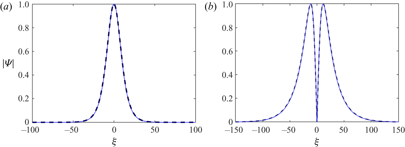
 $2\,\%$, implying that the asymptotic solution is accurate. This accuracy is also demonstrated in figure 5 where the absolute value of
 $\varPsi$ is plotted as a function of
 $\xi$ at
 $y=0$. The maximum of the disturbance is concentrated at the maximum amplitude of the isobath deviation, i.e. at
 $\xi =0$ and then decays exponentially in the far field as
 $\exp (- k_{r}\xi )$ where
 $k_{r}$ is the real part of the wavenumber of the corresponding decaying mode in the far field.
The envelope of the pressure fluctuations,  $|\varPsi |$, as a function of
 $\xi$ at
 $y=0$ generated by the numerical method (solid line) and the asymptotic method (dashed line) for the (1,1) and (2,1) modes, for the full problem for parameters
 $b=2$,
 $\alpha =-1.5$ and
 $\epsilon =0.1$.

The trapped frequencies  $\omega$ as calculated from the asymptotic method and a comparison of
 $\omega _{2}$ from the asymptotic method,
 $\omega _{2}^{A}$, and the numerical method,
 $\omega _{2}^{N}$. Here
 $\alpha =-1.5$,
 $b=2$ and
 $\epsilon =0.1$.

These tCSWs all lie within the continuous spectrum and since they decay to zero exponentially in the far field, no energy leaks from the region of trapping. To demonstrate that they do not project to the Kelvin wave, note the orthogonality relation (Proudman Reference Proudman1929)
 \begin{equation} \iint H(u_{i}u_{j}+ v_{i}v_{j})\,\textrm{d} x\,\textrm{d} y+\frac{1}{R^2} \iint \eta_{i}\eta_{j}\,\textrm{d} x\,\textrm{d} y=\delta_{i,j}E_{j}, \end{equation}
where  $u_{l}$,
 $v_{l}$,
 $\eta _{l}$, for
 $l=i,j$ are the horizontal velocities and the surface displacement, respectively, for any two solutions of (2.9) subject to the b.c.s (2.5) and (2.7),
 $E_{i}$ is twice the energy associated with the
 $i$-th mode which is given by (4.41) with
 $j=i$ with the integrals evaluated over the channel. Substituting the Kelvin wave (that is concentrated along the coast) and the trapped CSW into (4.41), and evaluating the integrals numerically gives that the right-hand side of (4.41) is
 $O(10^{-10})$ which implies that the trapped mode is orthogonal to the Kelvin wave.
5. Open ocean
It has been shown in this work that CSWs can be trapped for an infinitely long channel of variable bathymetry. In order to extend these results to an open ocean and also check the validity of the approximate condition at the shelf–ocean boundary, the full equation (2.9) subject to the b.c.s (2.5) and (2.6a,b) is solved numerically. Consider the depth profile,
 \begin{align} H(x,y)=\begin{cases} 1-(1-H_{0})\exp(-(y^{2}-p(x)^{2})^{-s}+p(x)^{-2s}), & 0\leq y\leq p(x),\\ 1, & y\geq p(x), \end{cases} \end{align}
where  $p(x)=(1+\alpha \epsilon ^{2}\textrm {sech}^{2}\epsilon x)/(1+\alpha )$. The depth at the coast is
 $H_{0}$ and the depth in the ocean is 1. Here
 $\alpha >0$ corresponds to the submerged ridge case and
 $\alpha <0$ to the submerged valley case. The numerical method of Appendix A shows that only the submerged ridge topography admits trapped modes. For the numerical method here, a Hermite interpolant is employed in the
 $x$ direction and a Laguerre interpolant in the
 $y$ direction. This cubic eigenvalue problem is linearised and the b.c.s are imposed following appendix C.
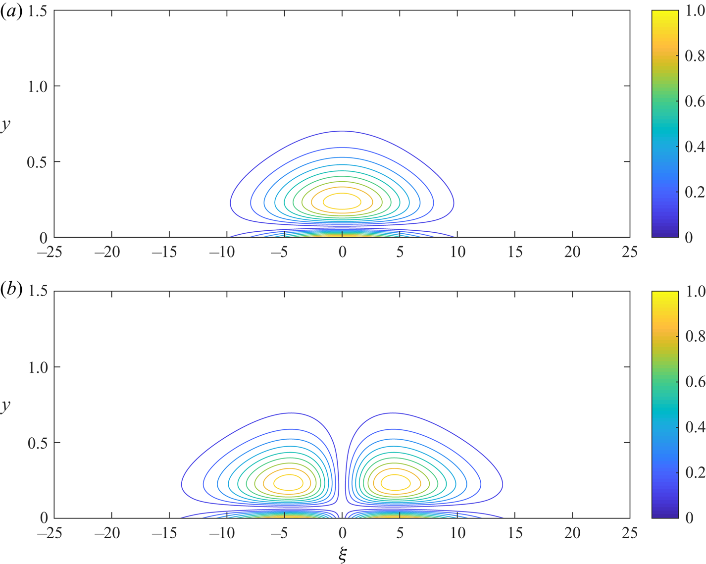
Trapping of the  $\omega _{1,1}$ and
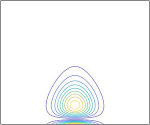
 $\omega _{2,1}$ trapped modes is shown in figure 6. Most of the wave disturbance is concentrated along the submerged ridge and the modes decay in the far field both along and away from the coast. The approximate b.c. (2.7), which enabled the reduction of the problem to a channel with solid walls in § 4, is evaluated by imposing this b.c. at
 $y=L_{y}$, by using a Chebyshev interpolant in the cross-shore direction. We set
 $L_{y}=\max P(x)$, which corresponds to the shelf–ocean boundary, and then gradually increase
 $L_{y}$ to infinity, which should imply that the frequency of tapping,
 $\omega _{L}$, should converge to the frequency of trapping,
 $\omega$, for the unapproximated open-ocean b.c. We also investigate whether demanding that the tangential velocity vanishes at the shelf–ocean boundary, i.e.
 $\textrm {i}\omega \eta _{x}-\eta _{y}=0$, can also serve as an approximate b.c. (with corresponding frequency of trapping denoted by
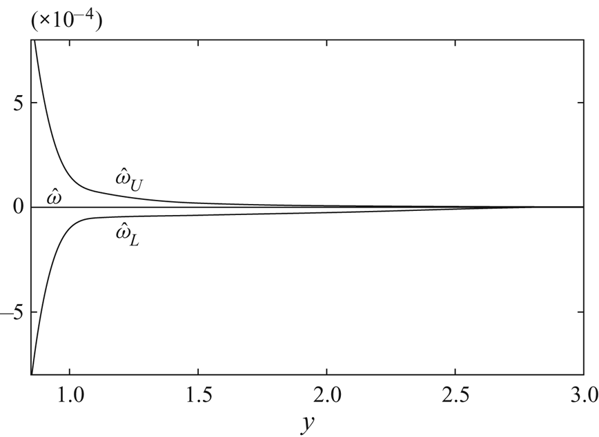
 $\omega _{U}$). For the rigid-lid case it is known that these two approximations at the shelf–ocean boundary (requiring the normal or the tangential component of the velocity to vanish) give a lower and an upper bound to the frequency of trapping (Johnson Reference Johnson1989; Kaoullas & Johnson Reference Kaoullas and Johnson2012). Denote the scaled (lower and upper) frequencies of trapping by
 $\hat {\omega }_{i}=\omega _{i}/\omega -1, i=L,U$, and
 $\hat {\omega }=0$ is the (scaled) frequency of the unapproximated problem. It is demonstrated in figure 7 that both
 $\hat {\omega }_{L}$ and
 $\hat {\omega }_{U}$ converge to
 $\hat {\omega }$ as
 $L_{y}$ increases. Thus, similarly to the rigid-lid case, we have the following bounds to the frequency of trapping:
 \begin{equation} \omega_{L}\leq\omega\leq\omega_{U}. \end{equation}
The stream function amplitude,  $|\varPsi |$ of (a) the (1,1) mode and (b) the (2,1) mode for the open-ocean case. Here,
 $b=2$,
 $\alpha =0.2$ and
 $\epsilon =0.1$.

Lower  $(\hat {\omega }_{L})$ and upper bounds
 $(\hat {\omega }_{U})$ for the frequency of trapping
 $\hat {\omega }$ of the (1,1) mode for increasing
 $L_{y}$.

6. Discussion
It is well known that in the rigid-lid limit (Kaoullas & Johnson Reference Kaoullas and Johnson2012; Rodney & Johnson Reference Rodney and Johnson2015) alongshore variations in the topography can lead to CSWs being trapped both away and along the coast. Here, a regular asymptotic expansion method has been presented to investigate whether similar shelf geometries can still support tCSWs when the rigid-lid assumption is relaxed. Mathematically, this is a nonlinear eigenvalue problem for the spectral parameter, that is the frequency,  $\omega$, which also appears in the b.c.s. The presence of the Kelvin wave at all frequencies implies that the spectrum of the operator is everywhere continuous and if any trapped mode exists, it will be embedded in the continuous spectrum (similarly to the water wave problem in Aslanyan et al. (Reference Aslanyan, Parnovski and Vassiliev2000)).
A waveguide with impermeable sidewalls is considered and the scale of the alongshelf variations of the isobaths is taken to be large, compared with the shelf width. It is shown that in the case of a submerged ridge, trapping is always possible even when the depth is perturbed only slightly while in the case of a submerged valley, no trapping is possible. The rigid-lid case follows immediately and it is shown that the frequencies of trapping for the pressure formulation here are in excellent agreement with the stream function formulation of Kaoullas & Johnson (Reference Kaoullas and Johnson2012) and Rodney & Johnson (Reference Rodney and Johnson2015). The accuracy of this method is demonstrated by comparing the asymptotic results with the numerical results of a pseudospectral method, which shows that the asymptotic method is extremely accurate. Additionally, the numerical method is also used to demonstrate that trapped modes continue to exist when the shelf extends into the open ocean, thus removing the approximation taken at the shelf–ocean boundary.
It is generally accepted that the main mechanism of excitation of CSWs is the wind stress (see Adams & Buchwald Reference Adams and Buchwald1969) of a comparable period. In the rigid-lid limit, it has been shown in Rodney & Johnson (Reference Rodney and Johnson2015) that tCSWs can also be generated by wind-stress forcing, even when applied in the far field. Without continuous forcing these trapped modes would be eventually be destroyed by dissipation.
The presence of stratification could alter the characteristics of CSWs significantly, since the wave frequency increases at all alongshore wavenumbers (Mysak Reference Mysak1980; Brink Reference Brink1991). For a shelf with sufficiently strong stratification, the group velocity is generally in the same direction as the phase velocity and at high wavenumbers the wave frequency increases monotonically to the inertial frequency  $f$. The short waves carrying energy in the opposite direction of long waves disappear and so trapping is impossible. For sufficiently weak stratified shelves, however, some subinertial waves remain evanescent (Huthnance Reference Huthnance1978; Chapman Reference Chapman1983), and as shown in Rodney & Johnson (Reference Rodney and Johnson2012) (in the rigid-lid case) trapping is possible in a reduced range of frequencies.
Acknowledgements
This work was co-funded by the European Regional Development Fund and the Republic of Cyprus through the Research and Innovation Foundation (project: POST-DOC/0916/0138)
Declaration of interests
The authors report no conflict of interest.
Appendix A. Numerical solution for a rectilinear shelf
Following Kaoullas & Johnson (Reference Kaoullas and Johnson2010a) we cast (3.1) into a linear eigenvalue problem for  $k$ with the following transformation
 $Y=kZ$ to give:
 \begin{gather} Z^{\prime\prime}+H^{\prime}/(H)Z^{\prime} +H^{\prime}/(H\omega)Y+(\omega^{2}-1)/(HR^2)Y=kY, \end{gather}
 \begin{gather}Y=kZ, \end{gather}
subject to (3.2) and (3.3) or (3.4a,b). We discretise (A 1) on a Chebyshev grid of  $N$ points following Trefethen (Reference Trefethen2000) and using the appropriate differentiation matrices we get the linear eigenvalue problem
 \begin{equation} \begin{pmatrix} \boldsymbol{A_{1}} & \boldsymbol{A_{2}}(\omega) \\ \boldsymbol{I} & \boldsymbol{0} \end{pmatrix}=k \begin{pmatrix} \boldsymbol{Y} \\ \boldsymbol{Z} \end{pmatrix}, \end{equation}
where  $\boldsymbol {A_{1}}$ and
 $\boldsymbol {A_{2}}(\omega )$ are the discrete form of the left-hand side of (A 1). To impose the b.c. (3.2) at the coast
 $-\omega Y^{\prime }=kY$ we replace the last rows of
 $\boldsymbol {A_{1}}$ and
 $\boldsymbol {A_{2}}(\omega )$ with the last row of the Chebyshev differentiation matrix times
 $-\omega$. It is worth noting that a similar condition applies for
 $Z$, that is
 $-\omega Z^{\prime }=kZ$ which is imposed by replacing the last rows of
 $\boldsymbol {I}$ and
 $\boldsymbol {0}$ in a similar manner. Imposing this b.c. ‘twice’ results in a much better conditioned matrix, and also removes some spurious eigenvalues. The approximate b.c. (3.3) is imposed in exactly the same manner (the first rows are replaced now) to give an
 $N$
 $\times$
 $N$ linear eigenvalue problem to be solved by standard numerical packages for each set value of the frequency
 $\omega$.
The open ocean unapproximated b.c. (3.4a,b) is imposed by removing the first row and column of each matrix in (A 3) thus giving an  $N-2$
 $\times$
 $N-2$ linear eigenvalue problem.
Appendix B. Asymptotic solution in the rigid-lid case
The leading-order equation is
 \begin{gather} (h\varPsi^{c}_{y})_{y}+h (2b\mu/\omega_{0}-\mu^{2})\varPsi^{c}=0, \end{gather}
 \begin{gather}\omega_{0}\varPsi^{c}_{y}+\mu\varPsi^{c}=0,\quad y=0,1. \end{gather}
This equation is close to the stream function formulation in Kaoullas & Johnson (Reference Kaoullas and Johnson2012), with  $h$ appearing as
 $h^{-1}$ and also the b.c.s (B 2) replacing Dirichlet conditions. The solution of (B 1) satisfying (B 2) is
 \begin{equation} \varPsi^{c}=C \,\textrm{e}^{-by}\left(\cos\lambda y+ I \sin\lambda y\right), \end{equation}
where
 \begin{equation} \lambda^{2}=\frac{2b\mu}{\omega_{0}}-b^2-\mu^2=\frac{b^2}{\omega_{0}^{2}}-b^2,\quad I=\frac{b\omega_{0}-\mu}{\omega_{0}\lambda}=-\frac{\lambda}{b}, \quad C=\sqrt{2}\omega_{0}\,\textrm{e}^{b},\quad \lambda=n{\rm \pi} \end{equation}
and
 \begin{equation} b=k_{0}\omega_{0}=\mu\omega_{0}. \end{equation}
The first term of (B 4) is the dispersion relation for the unperturbed channel, as in the stream function formulation. Even though the two differential operators are different, their spectrum is the same, as expected, since the underlying physical problem, (i.e. the rigid-lid case) is the same. At the next order:
 \begin{gather} (h\varPsi_{1_{y}})_{y}+ (2b\mu/\omega_{0}-\mu^{2})h\varPsi_{1} -(2 b\mu\omega_{1}/\omega_{0}^{2})h\varPsi^{c}f_{0}=0, \end{gather}
 \begin{gather}\textrm{i}\omega_{0}\varPsi_{1_{y}}+\textrm{i}\mu\varPsi_{1}+\textrm{i}\omega_{1}f_{0}\varPsi^{c}_{y}+f_{0_{\xi}}\varPsi^{c}=0,\quad y=0,1. \end{gather}
The solvability condition becomes
 \begin{equation} 2\omega_{1}(\mu^{2}/\omega_{0})f_{0}=0, \end{equation}
which immediately forces  $\omega _{1}=0$. Now
 $\varPsi _{1}$ is the solution of
 \begin{gather} \varPsi_{1_{yy}}+2b\varPsi_{1_{y}}+\left(2b\mu/\omega_{0}-\mu^{2}\right)\varPsi_{1} = 0, \end{gather}
 \begin{gather}\omega_{0}\varPsi_{1_{y}}+\mu\varPsi_{1}=\textrm{i} f_{0_{\xi}}\varPsi^{c},\quad y=0,1, \end{gather}
giving
 \begin{equation} \varPsi_{1}=C \,\textrm{e}^{-by}\left(\cos\lambda y+ I \sin\lambda y\right)f_{1}(\xi)+ (\textrm{i} C/\omega_{0}\lambda) \,\textrm{e}^{-by}\sin\lambda y f_{0_{\xi}}. \end{equation}
The order  $\epsilon ^{2}$ equation is
 \begin{align} & (h\varPsi_{2_{y}})_{y}+ (2b\mu/\omega_{0}-\mu^{2})h\varPsi_{2}- (2 b\mu\omega_{2}/\omega_{0}^{2})h\varPsi^{c}f_{0}+ f_{0_{\xi\xi}}\varPsi^{c}\nonumber\\ &\quad +\alpha \gamma 2b(1-2y)(\varPsi^{c}_{y}+(\mu/\omega_{0})\varPsi^{c})f_{0}=0, \end{align}
 \begin{equation} \textrm{i}\omega_{0}\varPsi_{2_{y}}+\textrm{i}\mu\varPsi_{2}+\textrm{i}\omega_{2}f_{0}\varPsi^{c}_{y}+\varPsi_{1_{\xi}}=0,\quad y=0,1. \end{equation}
Multiplying (B 12) by  $\varPsi ^{c}$ and integrating gives
 \begin{equation} I_{1}f_{0_{\xi\xi}}+V(\xi)f_{0}=\omega_{2}I_{2}f_{0}, \end{equation}
where
 \begin{align} V(\xi) &= \alpha \gamma2b\int_{0}^{1} h(1-2y)(\varPsi^{c}\varPsi^{c}_{y}+(\mu/\omega_{0})\varPsi^{c2}) \nonumber\\ &=-2 b\alpha \gamma, \end{align}
 \begin{equation} I_{1}=1,\quad I_{2}=2\mu^{2}/\omega_{0}.\end{equation}
Since the sign of the potential  $V$ depends solely on
 $\alpha$, it can be determined from (4.34) that trapped modes exist only when
 $\alpha <0$ (submerged ridge). The analysis here for a rigid-lid can be followed in terms of the stream function instead of the pressure and, as expected, leads to the same expressions (B 14), (B 15) and (B 16).
Appendix C. Numerical solution for a non-rectilinear shelf
The waveguide in § 4 is truncated to a rectangular, discretised domain, forming a grid with  $M$ points in the
 $x$ direction and
 $N$ points in the
 $y$ direction. Introducing the column vector
 $\boldsymbol {p}$ as the discrete values of
 $\varPsi$ on the rectangular domain, (4.39) can be written in its discrete form as,
 \begin{equation} \omega^{4}\boldsymbol{A}\boldsymbol{p}+\omega^{2}\boldsymbol{B}\boldsymbol{p}+\omega \boldsymbol{C}\boldsymbol{p}+\boldsymbol{E}\boldsymbol{p}=\boldsymbol{0}, \end{equation}
where the  $MN$
 $\times$
 $MN$ matrices are given by
 \begin{gather} \boldsymbol{A}=1/(\boldsymbol{H}R^{2}), \end{gather}
 \begin{gather}\boldsymbol{B}=\boldsymbol{D}^{2}_{x}+\boldsymbol{D}^{2}_{y}+2b(\boldsymbol{P}_{x} \boldsymbol{D}_{x}+\boldsymbol{P}_{y} \boldsymbol{D}_{y})-1/(\boldsymbol{H}R^{2}), \end{gather}
 \begin{gather}\boldsymbol{C}=2b\textrm{i}((\boldsymbol{I}-\boldsymbol{P}_{y})\boldsymbol{D}_{x}+ \boldsymbol{P}_{x}(\boldsymbol{D}_{y}+b\boldsymbol{I})), \end{gather}
 \begin{gather}\boldsymbol{E}=b^{2}(2\boldsymbol{P}_{y}-\boldsymbol{I}), \end{gather}
the matrices  $\boldsymbol {D}^{2}_{y}$ are
 $\boldsymbol {H}$, and
 $\boldsymbol {P}_{x}$,
 $\boldsymbol {P}_{y}$ are the discrete values of the topography function (4.8) and (4.10a,b). Finally, the differentiation matrices
 $\boldsymbol {D}^{i}_{y}$ and
 $\boldsymbol {D}^{i}_{x}$ for
 $i=1,2$ are the appropriate tensor products with the identity matrix, of the Chebyshev differentiation matrix and the Laguerre differentiation matrix, respectively, as defined in Weideman & Reddy (Reference Weideman and Reddy2000).
Accuracy can be greatly improved by shifting the frequency  $\omega$ to the cutoff frequency of the rectilinear shelf
 $\omega _{0}$ with
 $\omega =\omega _{0}+\lambda$ to give from (C 1),
 \begin{equation} \lambda^{4}\boldsymbol{A_{1}}\boldsymbol{p}+\lambda^{3}A_{2}\boldsymbol{p}+ \lambda^{2}\boldsymbol{A_{3}}\boldsymbol{p}+\lambda \boldsymbol{A_{4}}\boldsymbol{p}+ \boldsymbol{A_{5}}\boldsymbol{p}=\boldsymbol{0}, \end{equation}
where,
 \begin{gather} \boldsymbol{A_{1}}=\boldsymbol{A}, \end{gather}
 \begin{gather}\boldsymbol{A_{2}}=4\omega_{0}\boldsymbol{A}, \end{gather}
 \begin{gather}\boldsymbol{A_{3}}=6\omega_{0}^{2}\boldsymbol{A}+\boldsymbol{B}, \end{gather}
 \begin{gather}\boldsymbol{A_{4}}=4\omega_{0}^{3}\boldsymbol{A}+2\omega_{0}\boldsymbol{B}+\boldsymbol{C}, \end{gather}
 \begin{gather}\boldsymbol{A_{5}}=\omega_{0}^{4}\boldsymbol{A}+\omega_{0}^{2}\boldsymbol{B}+\omega_{0} \boldsymbol{C}+\boldsymbol{E}. \end{gather}
The b.c.s (4.40) now become
 \begin{equation} \lambda^{2}\boldsymbol{D}_{y}\boldsymbol{p}+\lambda(2\omega_{0}\boldsymbol{D}_{y}-\textrm{i}\boldsymbol{D}_{x}) \boldsymbol{p}+ (\omega_{0}^{2}\boldsymbol{D}_{y}-2\omega_{0}\textrm{i}\boldsymbol{D}_{x}+b\boldsymbol{I}) \boldsymbol{p}=\boldsymbol{0},\quad y=0,1, \end{equation}
and will be imposed on (C 6) by replacing the appropriate rows of matrices (C 7)–(C 11) for the corresponding power of  $\lambda$. Let us consider the
 $\lambda ^{4}$ case, which has the
 $\boldsymbol {0}$ matrix as a coefficient in (C 12). Here, to impose the b.c. at
 $y=1$ we need to replace the
 $1+(n-1)N,(n=1,\ldots ,M)$ rows of matrix
 $\boldsymbol {A_{1}}$ with the corresponding rows of the
 $\boldsymbol {0}$ matrix, and to impose the b.c. at
 $y=0$ we need to replace the
 $nN,(n=1,\ldots ,M)$ rows of these matrices. In a similar manner we can impose the b.c.s to the other matrix coefficients of (C 6). Finally, to linearise the fourth-order polynomial eigenvalue problem (4.40) to a generalised eigenvalue problem we introduce the following linearisation:
 \begin{equation} \boldsymbol{q}=\lambda\boldsymbol{p},\quad \boldsymbol{r}=\lambda\boldsymbol{q},\quad \boldsymbol{s}=\lambda\boldsymbol{r}, \end{equation}
to give
 \begin{equation} \begin{pmatrix} \boldsymbol{A_{5}} & \boldsymbol{A_{4}} & \boldsymbol{A_{3}} & \boldsymbol{A_{2}}\\ \boldsymbol{0} & \boldsymbol{I} & \boldsymbol{0} & \boldsymbol{0}\\ \boldsymbol{0} & \boldsymbol{0} & \boldsymbol{I} & \boldsymbol{0}\\ \boldsymbol{0} & \boldsymbol{0} & \boldsymbol{0} & \boldsymbol{I} \end{pmatrix} \begin{pmatrix} \boldsymbol{p} \\ \boldsymbol{q} \\ \boldsymbol{r} \\ \boldsymbol{s} \end{pmatrix}=\lambda \begin{pmatrix} -\boldsymbol{A_{1}} & \boldsymbol{0} & \boldsymbol{0} & \boldsymbol{0}\\ \boldsymbol{I} & \boldsymbol{0} & \boldsymbol{0} & \boldsymbol{0}\\ \boldsymbol{0} & \boldsymbol{I} & \boldsymbol{0} & \boldsymbol{0}\\ \boldsymbol{0} & \boldsymbol{0} & \boldsymbol{I} & \boldsymbol{0} \end{pmatrix} \begin{pmatrix} \boldsymbol{p} \\ \boldsymbol{q} \\ \boldsymbol{r} \\ \boldsymbol{s} \end{pmatrix}. \end{equation}
Even though it is a  $4MN$
 $\times$
 $4MN$ generalised eigenvalue problem, the matrices are very sparse and thus can be solved with any sparse eigenvalue finder routine.