Introduction
A bio-geochemical cycle was proposed by Charlson et al. (Reference Charlson, Lovelock, Andreae and Warren1987) that includes the production of dimethylsulphoniopropionate (DMSP), by phytoplankton enzymatic activity, a precursor compound to the volatile dimethyl sulphide (DMS, CH3SCH3). The release of DMS from the surface ocean, followed by both oxidation to non-sea salt sulphate (nss-SO42-) and methanesulphonic acid (MSA, CH3SO3H) formation, may act as cloud condensation nuclei (CCN) sources for marine cloud formation. Furthermore, this mechanism (named the ‘CLAW hypothesis’) became a potential link between the marine biogenic aerosols and climate changes. According to Andreae & Crutzen (Reference Andreae and Crutzen1997), changes in CCN concentration affect the concentration number of cloud droplet, which in turn influences cloud albedo and ultimately the climate. Additionally, numerous studies have already revealed that sulphate aerosols participate in the earth-atmosphere radiation budget by partially scattering and reflecting the incoming solar radiation (Langmann et al. Reference Langmann, Herzog and Graf1998, Kirkevag et al. Reference Kirkevag, Iversen and Dahlback1999).
Fine continental dust blown from the Patagonian semi-desert (McConnell et al. Reference McConnell, Aristarain, Banta, Edwards and Simões2007) together with non-sea salt sulphate particles constitute important sources to the total suspended aerosol concentration in the Southern Ocean. On King George Island (KGI), South Shetland Islands, located to the north-east of the Antarctic Peninsula tip (62°S, 58°W), terrigenous enriched aerosols of Al, Si, K, Fe, Ti, Mn and Sr were monitored by Correia et al. (Reference Correia, Artaxo and Maenhaut1998) between 1985 and 1993 at the Brazilian Antarctic station Comandante Ferraz (62°05′S, 58°23.5′W). Analysis of these data revealed no significant seasonal behaviour, but a structure formed by peaks of short duration and periods of low concentrations. In contrast, the total atmospheric S in the fine mode aerosol (aerodynamic diameter < 2.5 μm) presented marked intra-annual variability with a minimum (c. 50 ng m-3) in the midwinter (May–July) and a maximum (200 ng m-3) in summer (November–February). A similar behaviour was observed from Br measurements. Additionally, aerosol number concentrations (ANC), monitored at the same site, also exhibited a similar marked seasonal pattern as total S (Dalia et al. Reference Dalia, Evangelista, Simões and Pereira2004). The above patterns reinforce the findings of Fitzgerald (Reference Fitzgerald1991) who stated that the background aerosols in the boundary layer over remote oceans is of marine origin, and not aged continental. In addition, Vallina et al. (Reference Vallina, Simó and Gassó2006) have shown that in the Southern Ocean region satellite-derived AOD (aerosol optical depth), an indicator of CCN in the lower atmosphere, is positively correlated with satellite-derived chlorophyll a (chl a) concentration on a seasonal basis.
There are several regions in the Southern Ocean where remote sensing techniques and/or field measurements have estimated significant chl a concentrations (> 2 mg m-3): 1) the north-western Weddell Sea and Bellingshausen–Amundsen Sea (Moore & Abbott Reference Moore and Abbott2000), 2) the Scotia Sea (Holm-Hansen et al. Reference Holm-Hansen, Naganobu, Kawaguchi, Kameda, Krasovski, Tchernyshkov, Priddle, Korb, Brandon, Demer, Hewitt, Kahru and Hewes2004), 3) the Ross Sea (Pabi & Arrigo Reference Pabi and Arrigo2006), 4) the southern Chilean coast (Toro et al. Reference Toro, Paredes and Villagra1999), and 5) the Argentinean continental shelf (Gayoso Reference Gayoso2001, Saraceno et al. Reference Saraceno, Provost and Piola2005, Romero et al. Reference Romero, Piola, Charo and Garcia2006, Rivas Reference Rivas2006, Rivas et al. Reference Rivas, Dogliotti and Gagliardini2006, Signorini et al. Reference Signorini, Garcia, Piola, Garcia, Mata and McClain2006). In the last two decades, the marginal sea ice zone has also been recognized as a major area of intense primary production in the Southern Ocean (Lizotte Reference Lizotte2001). Large phytoplankton blooms occur in areas where the sea ice retreats periodically in the Weddell Sea (e.g. c. 60°S, 30°W). Nevertheless, a few phytoplankton species are recognized to have significant bio-geochemical impacts at the global climate scale. Particularly in the Southern Ocean, one can highlight the presence of diatoms and the haptophyte Phaeocystis sp. (mainly Phaeocystis antarctica Karsten) as major contributors to the regional primary productivity (Arrigo et al. Reference Arrigo, DiTullio, Dunbar, Robinson, van Woert, Worthen and Lizotte2000, Ditullio et al. Reference DiTullio, Grebmeier, Arrigo, Lizotte, Robinson, Leventer, Barry, van Woert and Dunbar2000, Garibotti et al. Reference Garibotti, Vernet, Ferrario, Smith, Ross and Quetin2003).
In remote regions, ANC components derive basically of particles from DMS oxidation, marine primary organic matter, marine secondary organic aerosols, sub-micron dust particles and sub-micron sea salt. A previous study by Crocker et al. (Reference Crocker, Ondrusek, Petty and Smith1995), of the Southern Ocean, has found an r 2 value between chl a and DMS concentrations of 0.356 (n = 30) for surface waters. DMS oxidation products such as MSA and SO4-2 particles are highly hygroscopic and exist predominantly in the size fraction ranging between 0.1 and 1 μm in diameter, which is the optimal size range for CCN formation. A spectral analysis applied to the elemental composition time series obtained at the study site (Correia et al. Reference Correia, Artaxo and Maenhaut1998) has not indicated any cyclic pattern. In contrast, surges of Al, Fe, Ca and Ti occurred randomly during all the seasons suggesting no evidence of a seasonal dust transport regime towards the Antarctic Peninsula, characterized by increases in the summer season. The same is valid for the wind intensity. On the other hand, DMS peaks during the summer season in several sub-Antarctic areas as compiled by Turner et al. (Reference Turner, Nightingale, Broadgate and Liss1995). Also, Vallina et al. (Reference Vallina, Simó and Gassó2006) have demonstrated that for the Southern Ocean (40–60°S), the seasonal CCN concentrations are characterized by a clear pattern of higher values during the summer and lowering towards the winter. Therefore, dust and sea salt variability at KGI cannot support the well marked interannual characteristic of ANC data.
Besides the geochemical parameters used as proxies of ocean primary productivity, related to the atmospheric measurements or ice core analysis, the variability of ANC may reflect the impact of biogenic and marine sources at the regional context of this work. Herein, we have investigated the correlation between ANC and chl a at four important productivity sites revealed by remote sensing (the Bellingshausen–Amundsen Sea, Weddell Sea, southern Argentinean continental shelf and southern Chilean waters) from September 1997–December 1998. During this time, the northern sector of the Antarctic Peninsula, where KGI is located, was subjected to the meteorological influences from all the above regions, due to the westerly winds, polar air masses and warmer air and moisture advection from South America (Turner Reference Turner2004). Besides that, inertial jet streams originating in the Weddell Sea are potentially responsible for considerable lowering of the air temperature in that region (Setzer & Harter Reference Setzer and Harter2004). Here a compilation of ocean-colour satellite images of Sea-viewing Wide Field-of-view Sensor (SeaWiFS), local wind databases obtained from an Automatic Weather Station (AWS), regional wind current charts compiled from NCEP/NCAR re-analysis, in combination with the ANC time-series obtained at KGI was conducted.
Study area
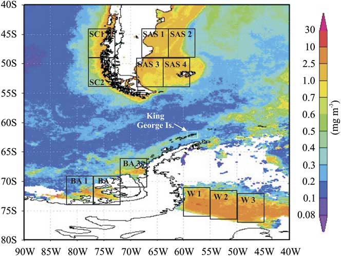
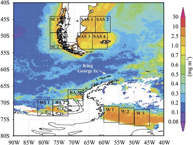
The study area covers the region between 40–80°S and 40–90°W in the Southern Ocean (Fig. 1). Atmospheric sampling of ANC was conducted at KGI where more than 92% of its area is ice covered and elevations reach approximately 700 m a.s.l. (Braun et al. Reference Braun, Saurer and Goßmann2004). According to Ferron et al. (Reference Ferron, Simões, Aquino and Setzer2004), considering the period from 1947–95, the mean annual temperature on this island was -2.8°C with a minimum of -5.2°C (1959) and a maximum of -0.8°C (1989).
Mean chl a concentration composite image obtained from SeaWiFS images, corresponding to the period September 1997–December 1998. Square boxes defined as BA1, 2, and 3 refer to Bellingshausen–Amundsen Sea sector; W1, 2, and 3 to Weddell Sea sector; SAS1, 2, 3, and 4 to southern Argentine shelf sector and SC1 and 2 to southern Chilean coast sector. KGI location is indicated by an arrow.
The Bellingshausen–Amundsen Sea sector comprises the longitude band from 130–60°W. It corresponds to an area of 8 x 10⁶ km2, which presents the second largest extent of frozen sea in West Antarctica during the summer season. The Weddell Sea sector (from 60–20°W) covers 12 x 106 km2 and is characterized by relatively cold ocean waters and large areas of perennial sea ice influenced by both the presence of a semi-permanent high pressure system and by polynyas, which result from katabatic winds derived from the Antarctic plateau (Gloersen et al. Reference Gloersen, Campbell, Cavalieri, Comiso, Parkinson and Zwally1992). The southern Argentinean shelf sector is located between 40–55°S in the Atlantic Ocean, while the southern Chilean coast sector comprises part of the southern Chilean coast (40–55°S at the Andean Pacific side).
Diatoms and haptophytes are abundant in the entire Southern Ocean but the relevant species involved in the DMS cycle have a geographically variable distribution, according to several authors. For instance, Phaeocystis antarctica (haptophyte) and Nitzschia subcurvata Hasle (diatom) are abundant in the Weddell Sea (Lizotte Reference Lizotte2001), whereas only P. antarctica predominates in the Bellingshausen–Amundsen Sea. In the southern Chilean coast sector, the most abundant diatom is Skeletonema costatum (Grev.) Cleve followed by Nitzschia closterium (Ehrenberg) W. Sm., Melosira sp. and several species of the genus Coconeis and Clavicula (Toro et al. Reference Toro, Paredes and Villagra1999). In the southern Argentinean shelf sector phytoplankton species vary both geographically and in time within the summer season (Gayoso Reference Gayoso2001), with the occurrence of Skeletonem costatum several Chaetoceros species, Phaeocystis spp. and Coccolithophorid species like Emiliania huxleyii (Loh.) Hay & Mohl., known as an important DMS producer. Still according to this author, in this region the phytoplankton distribution is dominated by seasonal occurrence of diatoms. In spring, the phytoplankton assemblage in the shelf-break was shown to be dominated by diatoms of the genus Thallasiosira and the haptophyte Phaeocystis sp., the latter particularly associated with high DMS production.
Databases and methods
Atmospheric sampling of ANC was conducted from September 1997–December 1998 on KGI at the atmospheric science module, located 1.8 km from the Comandante Ferraz station. The measurements of ANC were performed by a condensation nuclei counter, Model 3760 of TSI® Incorporated. Concentration values (in particle per cubic centimetre, N cm-3) were available at 10 minute intervals. The instrument allows detection of atmospheric particulates with diameters larger than 0.014 μm. Details on the operation and general characteristics of this equipment can be found in Maring & Schwartze (Reference Maring and Schwartze1994) and Dalia et al. (Reference Dalia, Evangelista, Simões and Pereira2004). Instrument failure interrupted the atmospheric sampling during October 1997.
Atmospheric samplings for ANC at the Argentine continental shelf were performed using a wind sector control system to prevent contamination from the ship’s exhaust. An aerosol inlet (a cylindrical tube of 20 cm length and 15 cm width) was used to protect the system from sea spray. It was positioned at the top of the ship (10 m a.s.l.), 50 m away from the ship stack’s emission, while the pumping unit and the condensation nuclei counter were installed inside the ship and consisted of one pump unit (one-head GAST model) and a wind sector sampling control, which is an electronic device connected to an anemometer (installed beside the inlet compartment), a data logger, a two-way electrical valve and pumps. It was internally programmed to interrupt the aerosol sampling any time the wind blew within an angular sector (named ‘dirty sector’) of 60° centred at a line between the inlet and the ship’s exhaust. This way, any time the wind blew into the inside of the ‘dirty sector’ the airflow connection between the filter holder and the pump was interrupted through a two-way electrical valve.
In order to obtain a latitudinal profile of atmospheric DMS (the most probable source of ANC over sea) in the south-western Atlantic and Southern Ocean, we performed measurements on board the Ary Rongel oceanographic vessel during the 2005 summer campaign. Air samples were concentrated in glass cartridges, containing 200/400 mg sorbent of coconut shell charcoal (SKC 226-09), installed in the inlet of a continuous air pumping system of controlled flux of 1 l min-1. Each flask was sealed after approximately 1° latitude integration on board. Extraction of DMS occurred under laboratory conditions at Rio de Janeiro State University, Brazil with the use of 1 ml of cold dichloromethane followed by 10 min ultrasound. DMS detection was performed by gas chromatography (Agilent 6890) with selective mass detector Agilent MSD 5973, making use of 1 μl of sample, in splitless mode, using helium as carrier gas at 1.0 ml min-1. Temperature profile of the chromatographic column was 40°C for 6 min, followed by a linear increase of 10°C min-1 until 200°C. Detection mode was the single ion monitoring SIM: 32, 71 and 86 m/z, with ionization source energy of 70 eV. Uncalibrated values attributed to DMS were based on the peak area obtained from the respective chromatogram.
Satellite-derived chl a concentration was obtained from SeaWiFS data, available at the NASA’s Goddard Space Flight Centre (GSFC) and Distributed Active Archive Centres (DAAC) at the ‘Giovanni Ocean Color Time Series Online Visualization and Analysis’ website (http://reason.gsfc.nasa.gov/OPS/Giovanni/ocean.aqua.shtml, accessed August 2006). The chl a SeaWiFS images (9 x 9 km2 resolution) were generated based on the global OC4v4 algorithm. SeaWiFS data acquisition in oceanic areas is constrained by cloud cover, sensor sensitivity and by seasonal sea ice cover. Chl a concentrations over the Bellingshausen–Amundsen Sea is generally available for the January–April and August–December periods. Databases for the period May–July are constrained by the absence of sunlight and sea ice formation. For the Weddell Sea, there was lack of information over the period April–October.
For the south-western Atlantic region, the NASA OC4v4 algorithm presented a reasonable performance (r 2 = 0.87) compared to the revised algorithm for south-western Atlantic data (Garcia et al. Reference Garcia, Garcia and McClain2005). At that site, despite the relatively low number of pairs of radiometric measurements, SeaWiFS estimations compare well with in situ chl a concentrations (0.77 < r 2 < 0.98, n = 21). Regarding the chl a concentration, an overall agreement was observed (r 2 = 0.77, n = 28), with a mean absolute percentage difference of 66%, which is above the goal generally accepted of 35% for satellite ocean colour chlorophyll estimates.
We have performed regression and correlation analyses between the time-series of ANC measured at KGI and the time-series of chl a concentrations in the potential source areas (Bellingshausen–Amundsen Sea, Weddell Sea, southern Argentinean shelf and southern Chilean coast) separately. Therefore, sub-areas of equal size (square boxes in Fig. 1) were defined based on the regional mean chl a composite image corresponding to the atmospheric sampling period at KGI (from September 1997–December 1998). Dimensions and location of the boxes were also based on the total dimension of observed chl a patches. The time series for concentration at the i-th (i = 1, 2, 3, 4) area was obtained by the monthly average of the results among their boxes, in the following way: for the Bellingshausen–Amundsen Sea: BA1 (69–74°S, 77–82°W), BA2 (69–74°S, 72–77°W), and BA3 (66–71°S, 67–72°W), for the Weddell Sea: W1 (71–76°S, 55–60°W), W2 (71.5–76.5°S, 50–55°W), and W3 (72–77°S, 45–50°W), for the southern Argentinean shelf: SAS1 (44–49°S, 63–68°W), SAS2 (44–49°S, 58–63°W), SAS3 (49–54°S, 64–69°W), and SAS4 (49–54°S, 59–64°W) and finally for the southern Chilean coast: SC1 (44–49°S, 73–78°W), and SC2 (49–54°S, 73–78°W).
The synoptic scale atmospheric transport of aerosols from the four postulated source areas to KGI was inferred on the basis of monthly regional surface wind current diagrams compiled from NCEP/NCAR re-analysis (Kalnay et al. Reference Kalnay, Kanamitsu, Kistler, Collins, Deaven, Gandin, Iredell, Saha, White, Woollen, Zhu, Leetmaa, Reynolds, Chelliah, Ebisuzaki, Higgins, Janowiak, Mo, Ropelewski, Wang, Jenne and Joseph1996, Kistler et al. Reference Kistler, Kalnay, Collins, Saha, White, Woollen, Chelliah, Ebisuzaki, Kanamitsu, Kousky, van den Dool and Fiorino2001). Additionally, an AWS (62°05′08′′S, 58°23′37′′W, 20 m a.s.l.) installed at the Comandante Ferraz station provided intensity and direction of wind data. The in situ meteorological records were compared with NCEP/NCAR data in order to evaluate differences between the local wind structure, which is induced by geomorphology and katabatic effects, and the regional wind pattern. Meteorological data used here was downloaded from http://antartica.cptec.inpe.br/ (accessed November 2006).
Results and discussion
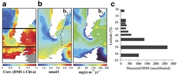
Modelled and in situ databases of atmospheric DMS and CCN at the Southern Ocean show that the parameters covariate significantly (Vallina et al. Reference Vallina, Simó and Gassó2006). This suggests that DMS may significantly contribute to CCN burden in that region (Vallina et al. Reference Vallina, Simó, Gassó, De Boyer-Montégut, Del Río, Jurado and Dachs2007). The latitudinal profile of atmospheric DMS from Rio de Janeiro, through the Patagonian continental shelf, up to King George Island on the northern Antarctic Peninsula, including the oligotrophic environments of the subtropical south-western Atlantic to high productivity regions of the Southern Ocean, resulted in substantial increase of DMS concentrations between latitudes 48° and 50°S (Fig. 2) well in accordance with modelled DMS proposed by Kloster et al. (Reference Kloster, Feichter, Maier-Reimer, Six, Stier and Wetzel2005). At a close sub-Antarctic site, DMS was measured by other authors. Turner et al. (Reference Turner, Nightingale, Broadgate and Liss1995) performed two simultaneous cruises through the Drake Passage to the Bellingshausen Sea from October–December 1992. Overall, average surface water concentrations for DMS was 2 nM (0.15–27 nM). In situ measurements of DMS and methane sulphonic acid (MSA) at Halley Station, Antarctica (75°S, 26°W) were conducted during February 2004–February 2005. During that period, DMS was observed in the atmosphere at Halley all year around (average 38.1 ± 43 pptv) with a maximum monthly average value of 113.6 ± 52 pptv in February 2004 coinciding with a minimum in sea ice extent. MSA was generally low throughout the year, with an annual average of 42 ng m-3, however MSA/nss-SO4-2 ratios were high implying a dominance of the addition oxidation route via DMS (Read et al. Reference Read, Lewis, Bauguitte, Rankin, Salmon, Wolff, Saiz-Lopez, Bloss, Heard, Lee and Plane2008).
a. Correlation map between monthly aqueous DMS concentrations from Kettle & Andreae (Reference Kettle and Andreae2000) and monthly chl a from SeaWiFS, 2002–04 (based on Vallina et al. 2006). b1. Modelled annual mean DMS atmosphere flux (based on Kloster et al. Reference Kloster, Feichter, Maier-Reimer, Six, Stier and Wetzel2005). b2. Modelled annual mean DMS surface concentrations (based on Kloster et al. Reference Kloster, Feichter, Maier-Reimer, Six, Stier and Wetzel2005). c.In situ DMS measurements (this work). Dashed line is the vessel track.

Concerning the ANC measured at KGI, the mean value (± 1 standard deviation) from September 1997–December 1998 was 2.3 ± 1.2 x 10³ N cm-3 (minimum of 0.7 x 10³ N cm-3 in September 1997 and maximum of 4.4 x 10³ N cm-3 in December 1998). One important feature of ANC over KGI is its well-defined seasonal variability (Fig. 3). Lower ANC values occur during the winter (March–September) while peaks coincide with the summer (approximately October–February). This result is consistent with DMS and MSA increases during spring–summer seasons observed during the cruise of the RRS Bransfield between 2 October 1992 and 10 January 1993 that covered a geographical area which included the Falkland Islands (Islas Malvinas), the Antarctic Peninsula and the Weddell Sea (Davison et al. Reference Davison, O’Dowd, Hewitt, Smith, Harrison, Peel, Wolff, Mulvaney, Schwikowski and Baltensperger1996).
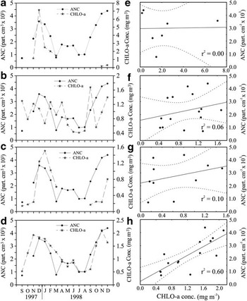
The left column shows superimposed monthly ANC at KGI and chl a for a. the Weddell Sea, b. the southern Chilean coast, c. the Bellingshausen–Amundsen Sea, and d. the southern Argentine shelf. The right column shows regression between ANC and chl a from e. the Weddell Sea, f. the southern Chile coast, g. the Bellingshausen–Amundsen Sea and h. the southern Argentine shelf, with corresponding 95% confidence bands.

Chl a concentrations were not available for all Antarctic circumpolar regions, especially in the Bellingshausen–Amundsen and Weddell seas due to sea ice expansion during the winter season and partially during spring and autumn. The average chl a concentration in the Weddell Sea sector was 2.1 ± 2.4 mg m-3, peaking in December 1997. As shown in Fig. 3a, no chl a values were available in the Weddell Sea between April and October 1998. Chl a concentrations in the Bellingshausen–Amundsen Sea sector were much lower compared to the Weddell Sea values, with a mean value of 0.6 ± 0.5 mg m-3, peaking in January. Considering the selected sub-areas in the Bellingshausen–Amundsen Sea sector, no chl a concentration data was available for the period April–August 1998, in contrast to the sites located further north (the southern Chilean coast and the southern Argentinean shelf) where chl a databases are available continuously. For the southern Chilean coast sector, mean concentration was 0.4 mg m-3 (Fig. 3b) peaking in September with a secondary peak in December, while in the southern Argentinean shelf sector a mean of 1.2 ± 0.6 mg m-3 (Fig. 3d) was found and a peak in November. Chl a concentration was highest in the Weddell Sea sector with values four times higher than the other selected regions, followed by the southern Argentinean shelf sector. The Spearman rank correlation coefficients (r S) obtained between ANC on KGI and chl a concentrations from the Weddell Sea, the southern Chilean coast, the Bellingshausen–Amundsen Sea and the southern Argentinean shelf were r S = -0.29 (n = 7), r S = +0.31 (n = 15), r S = +0.48 (n = 10), r S = +0.76 (n = 15), respectively (Fig. 3e–h) and only in the southern Argentinean shelf sector was statistically significant (P < 0.05).
From the correlation coefficients depicted in Fig. 3e–h, the higher value was attributed to chl a occurrence at the southern Argentinean shelf region and the atmospheric ANC suspended at KGI. Chl a inferred from the three other regions were not significantly correlated with ANC measured at KGI. The absence of chl a production around the Antarctic Peninsula during several months of the winter due to both sea ice cover and darkness suggest that the ANC background at KGI during the winter can be attributed to the biological production occurring in the northern sectors. Each of the four selected regions presented particular frequency data distribution characteristics. In the Weddell Sea and the southern Chilean coast (Fig. 3a & b) maximum chl a concentrations were characterized by rapid transient peaks at the beginning of the summer (November–December 1997). Particularly in the southern Chilean coast it was skewed to the month of September in 1997. On the other hand, both the Bellingshausen–Amundsen Sea and the southern Argentinean shelf sectors (Fig. 3c & d) presented a peak of concentration smoothed during the summer. The season of maximum concentrations in these regions lasts for about 3–4 months (beginning in November), similar to ANC time variation. Focusing on the seasonal variability of ANC, we found that chl a pattern in the southern Argentinean shelf sector can explain the general behaviour of that parameter measured on KGI between 1997 and 1998 (Fig. 3).
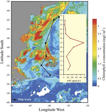
During the 2008 oceanographic cruise (from 23–27 October) we performed in situ ANC measurements specifically at the Patagonian continental shelf (within the latitudinal band of c. 38–60°S) in order to establish a direct comparison with regional chl a images for the corresponding period. In this case, the onboard cloud condensation counter was the same instrument employed for the KGI monitoring. Figure 4 depicts a chl a image from an eight days composite using SeaWiFS data between 23 and 30 October 2008 (the eight days window allowed elimination of most of the clouds). Data was downloaded at 0.1° x 0.1° resolution from the Giovanni server at NASA. The white line is the 200 m isobath, to visualize the shelf break. As one can see the values are quite high, with regions above 5 mg m-3. On board measurements indicated a significant increase of ANC in the vicinity of the central part of bloom occurrence, probably as a result of surrounding biological activity, which indicates that the Patagonian continental shelf chl a blooms are associated with significant ANC increases. From Fig. 4 a discrepancy of a few degrees of latitudes can be observed between the peak location and the bloom centre. This could be attributed to several processes such as the DMS oxidation time in the atmosphere prior to forming sulphate aerosols. Also, nucleation of new aerosols from sulphuric acid occurs mainly in the free troposphere and the production of CCN via this mechanism may take several days, involving the vertical transport of DMS, its oxidation, particle nucleation, growth and re-entrainment of particles into the boundary layer. Therefore, ANC increase due to this mechanism may happen downwind from the source (Woodhouse et al. Reference Woodhouse, Mann and Carslaw2008).
Chl a image from an 8 days (23–30 Oct 2008) composite using SeaWiFS from the Giovanni server at NASA. The solid black line is the approximate vessel route from Rio de Janeiro to King George Island and the white line is the 200 m isobath.

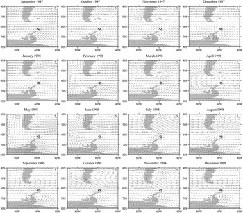
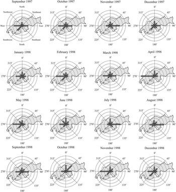
In order to explore the contribution of each potential source area to the apportionment of ANC measured on KGI, we have investigated the regional and local synoptic wind conditions during the sampling period. Figure 5 depicts the surface wind currents for each month provided by NCEP/NCAR re-analysis and Fig. 6 shows the in situ wind frequency distribution centred at the AWS installed on KGI. Figure 5 shows the regional influence of the sea level westerly winds (particularly between July and November) between southern South America and the tip of the Antarctic Peninsula, where KGI is located. This points to the potential influence of the southern Argentinean shelf and the southern Chilean coast regions with respect to the biogenic particles apportionment on KGI.
Regional monthly mean wind vectors at sea level compiled from NCEP/NCAR re-analysis between September 1997 and December 1998. Location of King George Island is indicated by a circle.

Wind frequency and direction from the AWS at King George Island during the period September 1997–December 1998. Concentric circles represent intervals of 10%.

Although the in situ meteorological data may be constrained by orographic aspects and katabatic winds, it can be used, roughly, to select geographical sectors associated with chl a (and presumably DMS production) potential source areas. It can be observed in Fig. 6 that on KGI the main synoptical influence derives from the zonal wind that blows through the Drake Passage, around latitude 60°S, from the Pacific to the Atlantic Ocean. The eastward direction also occurs with relatively high frequency and it is attributed to the clockwise cyclonic movement while they migrate through the region (Pereira Reference Pereira1990, Evangelista & Pereira Reference Evangelista and Pereira2002, Pereira et al. Reference Pereira, Evangelista, Pereira and Setzer2006).
During the monitoring period, south-east, south and north-east sectors contributed very little to the total frequency of winds observed on KGI, as indicated by Fig. 6. From this figure it can be observed that the two major frequency wind components are associated with the west and east directions. AWS data (Fig. 6) probably underestimate the southern Chilean coast contribution due to reasons presented above, while NCEP/NCAR re-analysis (Fig. 5) pointed out the higher influence of the southern Chilean coast associated with the westerly winds. The northern wind influence (the southern Chilean coast and the southern Argentinean shelf) comprised around 75% of the wind frequency reaching KGI. Also the lower influence of the Weddell Sea sector (c. 15%) was identified by both analyzed methods.
Despite the proximity of KGI to sub-Antarctic areas characterized by high ocean chl a concentration such as the Weddell and the Bellingshausen–Amundsen sea sectors, there is a considerably higher association between ANC measured on KGI in the low atmosphere and the ocean chl a concentration at the southern Argentinean shelf (the southern Chilean coast presented lesser correlation). Based on the data used in this study, a combination of high chl a concentration areas located at the northern latitudes of KGI associated with favourable wind circulation makes the southern Argentinean shelf and the southern Chilean coast regions potential contributors to the apportionment of marine derived aerosols (probably dominated by sulphates) over the South Shetland Islands.
Conclusions
Herein we have explored the understanding of ANC interannual variability on KGI and its association with marine productivity that may result in DMS oxidation products, marine primary organic matter (e.g. microcolloid aggregates) and secondary organic aerosols, all potential components of ANC. In this sense we suggest that chl a variability is the major process controlling the summer ANC seasonal peak, despite the inorganic compounds of terrigenous and marine sources. Our interpretations were based on the averaged monthly ANC data, which covered a period long enough to include secondary processes from chl a blooming to aerosol formation. A contribution of dust micro-particles eroded from the Argentine Patagonian semi-desert to the ANC, although not discarded, is probably of lesser importance to the annual variability, since the flux of dust into the southern latitudes is episodic (Evangelista et al. Reference Evangelista, Maldonado, Dos Santos, Godoi, Garcia, Garcia, Jonhson, Dias da Cunha, Leite, van Grieken, van Meel, Makarovska and Gaiero2010).
In this work, we employed a dataset of meteorological and environmental parameters in order to identify the main source regions of aerosol arriving at the northern tip of the Antarctic Peninsula (KGI), from September 1997–December 1998. From averaged SeaWiFS chl a images we selected four main potential source areas: the Bellingshausen–Amundsen Sea, the Weddell Sea, the southern Argentinean shelf and the southern Chilean coast. Correlations and associations among NCEP/NCAR regional wind pattern, local AWS wind data, monthly chl a concentration and aerosol number concentration allowed us to conclude that the southern Argentinean shelf region is more likely the main contributor of ANC (presumably through S particles) at KGI, despite the proximity of this island to Antarctic productive regions. We attribute the high correlation found to a combination of two factors: 1) the favourable regional surface wind circulation, and 2) the high occurrence of diatoms and the Coccolithophorid species like Emiliania huxleyii, which are known to be associated with high DMS emissions in the Southern Ocean.
Acknowledgements
Part of the images and data used in this study were acquired using the GES-DISC Interactive Online Visualization and Analysis Infrastructure (Giovanni) as part of the NASA’s Goddard Earth Sciences (GES) Data and Information Services Center (DISC). NCEP/NCAR re-analysis data was provided by the NOAA/OAR/ESRL PSD, Boulder, CO, USA, from their Web site at http://www.cdc.noaa.gov/. The authors would like to thank the Brazilian Antarctic Program (PROANTAR) and the Brazilian National Council for Scientific and Technological Development (CNPq) for logistical and financial support (Project 55.0353/02-0). We also thank CAPES (Coordenação de Aperfeiçoamento de Pessoal de Nível Superior) for funding scholarship. The constructive comments of the reviewers are also gratefully acknowledged.