Introduction
With the rapid development of 5G and 6G communications, beamforming technology has emerged and quickly been applied to multi-beam antennas, which shows the merits of increased communication coverage and system capacity, improved spectrum utilization, strong anti-interference and anti-fading ability [Reference Guo, Ansari and Fonseca1]. Typical implementation of beamforming technology is the circuit-based beamforming network, such as Nolen matrix [Reference Nolen2], Butler matrix [Reference Butler and Lowe3], and Blass matrix [Reference Blass4]. In past decades, there have been many studies on Butler matrices, including miniaturization [Reference Qiu, Zhu, Ouyang and Deng5, Reference Wang, Chen and Chu6], broadband [Reference Afifi and Sebak7, Reference Ma, Wu and Wang8], and filtering integration [Reference Shao, Chen, Chu and Lancaster9, Reference Shao, Chen, Wang, Chu and Lancaster10]. In addition to the Butler matrix, the Nolen matrix, which is an improved version of the Blass matrix, has received widespread attention in recent years [Reference Mosca, Bilotti, Toscano and Vegni11–Reference Tokos, Mylonas, Groumas, Katopodis, Gounaridis and Timens13] due to its flexibility and ability to avoid crossover.
However, most of the reports on beamforming networks exhibit equal power distribution at the output ports, resulting in significant sidelobe when connected to multi-beam antennas. For reducing sidelobe levels (SLL), beamforming networks with tapered distributions are preferred [Reference Park, Shin and Park14], for instance, the Chebyshev, Taylor, and binomial. Thus, techniques for realizing tapered distributions of beamforming networks have become major needs. Traditionally, the tapered amplitude distribution is achieved by connecting the beamforming network with unequal power dividers or directional couplers [Reference Gruszczynski, Wincza and Sachse15, Reference Shao and Chen16], and the SLL can be lower than −20 dB. However, since two-port power splitting circuit is used, the numbers of output ports in the beamforming network is inescapable increased, which increase the number of radiation elements. In Zhao et al. [Reference Zhao, Chu, Zhu and Guo17], by introducing the pattern-reconfigurable subarray controlled by the reconfigurable power dividers and couplers, improvement on SLL is obtained. But the increasement is limited (SLL = −12.1 dB). In Trinh-Van et al. [Reference Trinh-Van, Lee, Yang, Lee and Hwang18], two attenuators are connected to two output ports of a 4 × 4 Butler matrix for realizing tapered amplitude distribution without increasing the number of radiating elements, which achieves a peak SLL of −10.3 dB. Although low SLL can be realized, the above methods [Reference Gruszczynski, Wincza and Sachse15–Reference Trinh-Van, Lee, Yang, Lee and Hwang18] are all based on the connection of power splitting circuit instead of modifying the inherent feature of beamforming network for tapered distribution. Recently, beamforming network based on the generalized joined coupler (GJC) matrix is presented in Xu et al. [Reference Xu, Zhu and Guo19], which has the inherent characteristic for realizing low SLL. Two examples are implemented, including a 3 × 8 and a 3 × 7 beamforming network, where the SLLs are −18 dB and −15 dB, respectively. However, since the beamforming network in Xu et al. [Reference Xu, Zhu and Guo19] is a serial network, big phase difference errors will occur in the operated bandwidth, which results in beam squint when applied to antenna arrays.
In this article, a Chebyshev-distributed beamforming network with flat output phase performance is proposed for consistent beam pointing and low sidelobes applications, which mainly consists of two arbitrary-amplitude 4 × 4 Blass-like matrices and one 1 × 8 switch control circuit. In “Operating pronciples” section, the schematic of the beamforming network was introduced, and the working principles of the arbitrary-amplitude 4 × 4 Blass-like matrix and the 1 × 8 switch control circuit are analyzed in detail. In “Implementation and measurements”, an example was designed for verification and phase compensation method was adopted for obtaining minimum phase difference error in the bandwidth. Measurements indicate that the designed prototype has an output amplitude ratio of 0.143:0.341:0.71:1:1:0.71:0.341:0.143, which conforms to the Chebyshev distribution and can produce low SLL of −20 dB. Besides, the output port amplitudes and phase differences show good flatness. Conclusion is presented in section IV.
Operating principles
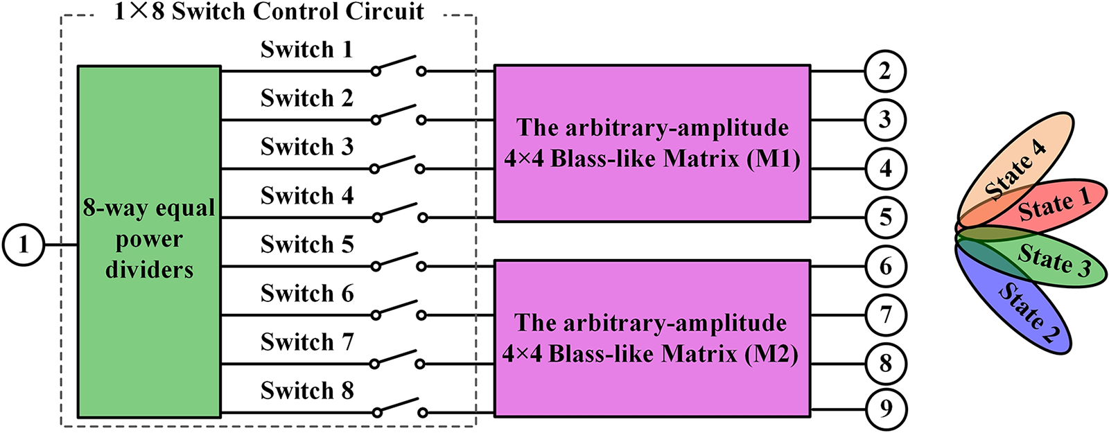
Figure 1 shows the schematic of the proposed Chebyshev-distributed beamforming network. It consists of one 1 × 8 switch control circuit and two arbitrary-amplitude 4 × 4 Blass-like matrices. The two arbitrary-amplitude 4 × 4 Blass-like matrices, named as M1 and M2, show symmetric amplitude distributions according to Chebyshev and exhibit the output phase differences of ±φ 1 and ±φ 2. The switching of the input ports of M1 is controlled by the switches 1–4. While the switches 5–8 are used for the controlling of the input ports of M2. By changing the on and off states of the eight switches, four beams can be formed.
Schematic of the proposed Chebyshev-distributed beamforming network.

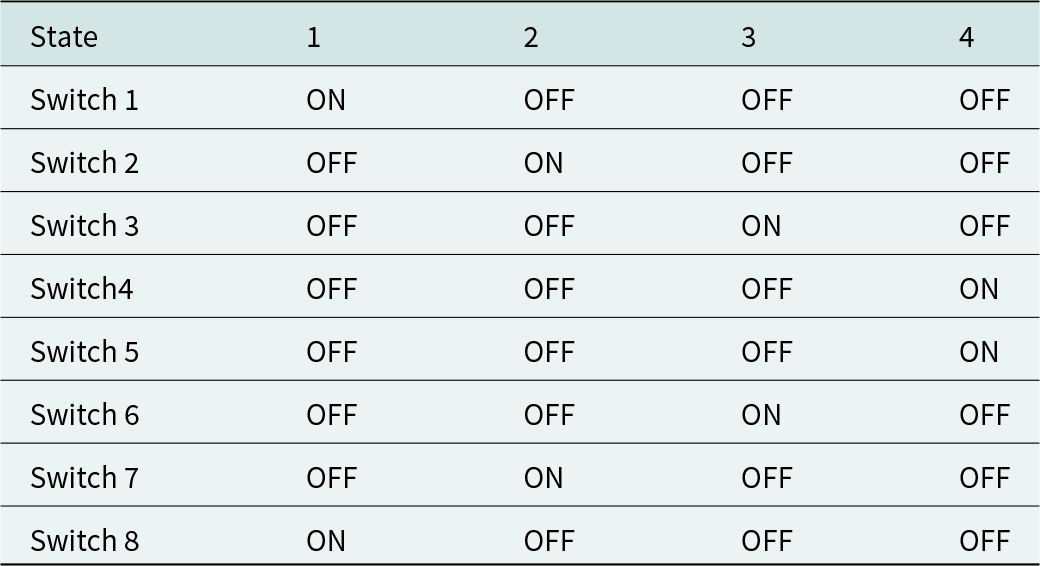
Table 1 gives the detailed information. When switches 1 and 8 are at the ON state and the other switches are at the OFF state (State 1), the 1 × 8 Chebyshev-distributed beamforming network shows an output phase difference of −φ 1. When switches 2 and 7 are at the ON state (State 2), the 1 × 8 Chebyshev-distributed beamforming network shows an output phase difference of φ 2. Similarly, when switches 3, 6 and switches 4, 5 are at the ON state (State 3 and 4), the Chebyshev-distributed beamforming network shows output phase differences of φ 1 and −φ 2, respectively. Thus, when connecting to a 1 × 8 array, beam pointing at four angles can be obtained. In the following, analysis of the arbitrary-amplitude 4 × 4 Blass-like matrix and the switch control circuit is introduced in order.
The relationship between beam and switches

Analysis of the arbitrary-amplitude 4 × 4 matrix
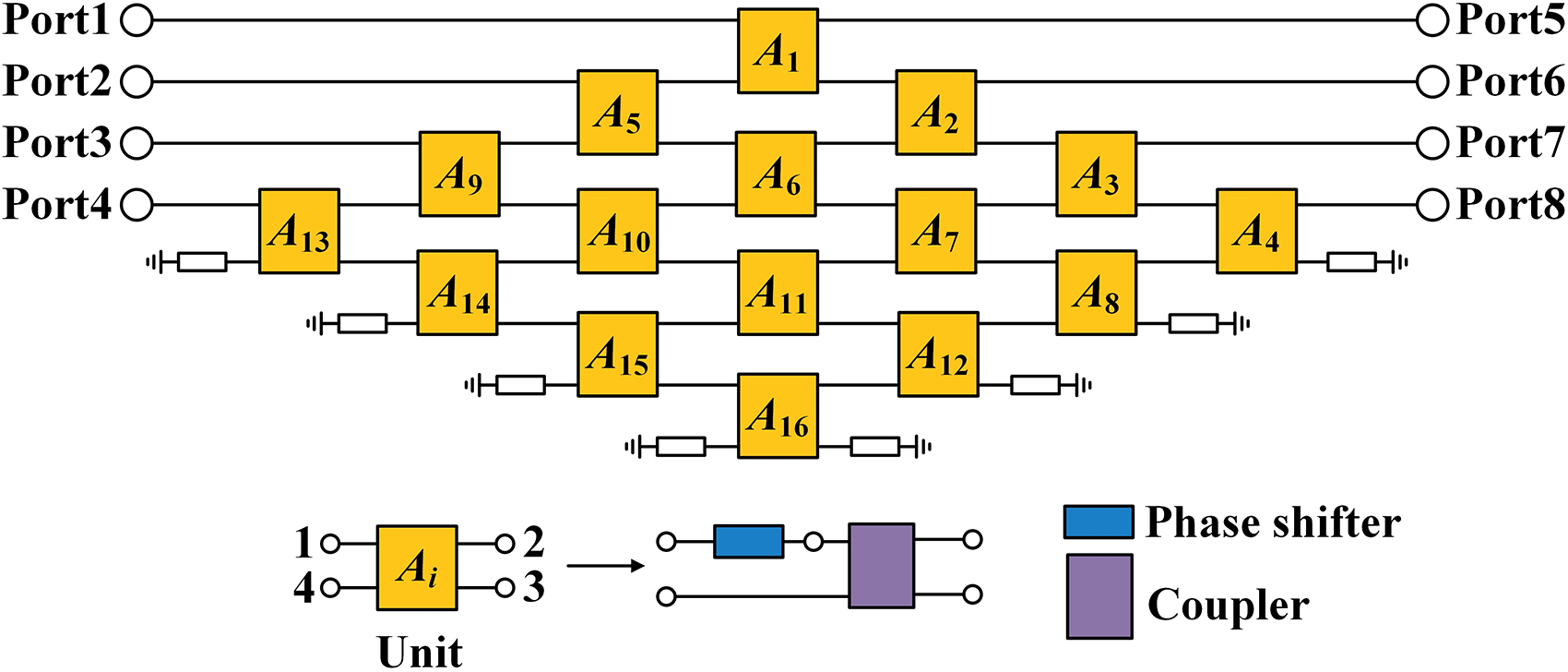
The diagram of the arbitrary-amplitude 4 × 4 matrix is shown in Fig. 2, where P1–P4 are input ports and P5–P8 are output ports. It merely consists of 16 units named as Ai (i = 1, 2, 3, ……16) and each unit is composed by one coupler cascaded with one phase shifter at the input port. The phase of each phase shifter is defined as θi, and the coupling coefficient of each coupler is defined as ki. It is noted that for generating arbitrary output amplitudes, the coupling port of the couplers in A 4, A 8, A 12, and A 16 unit is terminated to 50-Ω load. While the isolation port of the couplers in A 13–A 16 unit is also terminated to 50-Ω load. In the following, the relationships between the output distributions and the circuit performances are derived.
Diagram of the arbitrary-amplitude 4 × 4 blass like matrix.

Firstly, the four-port S-parameters of the unit Ai is expressed in (1). Based on (1), the S-parameters of the 4 × 4 matrix under different port excitations can be derived, as shown in (A1)–(A4) in the appendix. Thus, according to the output amplitude and phase difference, as well as the output phase of each coupler, the coupling coefficient of each coupler ki and phase of each phase shifter θi can be calculated.
 \begin{align}[{S_{Ai}}] & = \left[ {\begin{array}{*{20}{c}}
{{S_{i\_11}}}&{{S_{i\_12}}}&{{S_{i\_13}}}&{{S_{i\_14}}} \\
{{S_{i\_21}}}&{{S_{i\_22}}}&{{S_{i\_23}}}&{{S_{i\_24}}} \\
{{S_{i\_31}}}&{{S_{i\_32}}}&{{S_{i\_33}}}&{{S_{i\_34}}} \\
{{S_{i\_41}}}&{{S_{i\_42}}}&{{S_{i\_43}}}&{{S_{i\_44}}}
\end{array}} \right] \nonumber\\
& = \left[{\begin{array}{@{\,}c@{\,}c@{\,}c@{\,}c}
0&{\sqrt {1 - {k_i}} {e^{ - {\text{j}}({\alpha _i} - {\theta _i})}}}&{\sqrt {{k_i}} {e^{ - {\text{j(}}{\beta _i} - {\theta _i})}}}&0 \\
{\sqrt {1 - {k_i}} {e^{ - {\text{j}}({\alpha _i} + {\theta _i})}}}&0&0&{\sqrt {{k_i}} {e^{ - {\text{j}}{\beta _i}}}} \\
{\sqrt {{k_i}} {e^{ - {\text{j(}}{\beta _i} + {\theta _i})}}}&0&0&{\sqrt {1 - {k_i}} {e^{ - {\text{j}}{\alpha _i}}}} \\
0&{\sqrt {{k_i}} {e^{ - {\text{j}}{\beta _i}}}}&{\sqrt {1 - {k_i}} {e^{ - {\text{j}}{\alpha _i}}}}&0
\end{array}} \right]\end{align}
For better illustration, the detailed relationships between the output S-parameters and the circuit parameters under port 1 and 2 excitation are derived, as listed in (2) and (3). Then, the corresponding parameters related to the two states can be obtained, as shown in (4) and (5).
 \begin{align}\left\{ {\begin{array}{*{20}{l}}
{{S_{51}} = \sqrt {(1 - {k_1})} {e^{ - j({\theta _1} + {\alpha _1})}}} \\
{{S_{61}} = \sqrt {{k_1}(1 - {k_2})} {e^{ - j({\theta _1} + {\beta _1} + {\theta _2} + {\alpha _2})}}} \\
{{S_{71}} = \sqrt {{k_1}{k_2}(1 - {k_3})} {e^{ - j({\theta _1} + {\beta _1} + {\theta _2} + {\beta _2} + {\theta _3} + {\alpha _3})}}} \\
{{S_{81}} = \sqrt {{k_1}{k_2}{k_3}(1 - {k_4})} {e^{ - j({\theta _1} + {\beta _1} + {\theta _2} + {\beta _2} + {\theta _3} + {\beta _3} + {\theta _4} + {\alpha _4})}}}
\end{array}} \right.\end{align}
 \begin{align}\left\{ {\begin{array}{*{20}{l}}
{S_{52}} = \sqrt {(1 - {k_5}){k_1}} {e^{ - j({\theta _5} + {\alpha _5} + {\beta _1})}} \\
\begin{aligned}
{S_{62}} & = \sqrt {(1 - {k_5})(1 - {k_1})(1 - {k_2})} {e^{ - j({\theta _5} + {\alpha _5} + {\alpha _1} + {\theta _2} + {\alpha _2})}} \\
& \quad + \sqrt {{k_5}(1 - {k_6}){k_2}} {e^{ - j({\theta _5} + {\beta _5} + {\theta _6} + {\alpha _6} + {\beta _2})}} \\
{S_{72}} & = \sqrt {(1 - {k_5})(1 - {k_1}){k_2}(1 - {k_3})} {e^{ - j({\theta _5} + {\alpha _5} + {\alpha _1} + {\theta _2} + {\beta _2} + {\theta _3} + {\alpha _3})}}\\
& \quad + \sqrt {{k_5}(1 - {k_6})(1 - {k_2})(1 - {k_3})} {e^{ - j({\theta _5} + {\beta _5} + {\theta _6} + {\alpha _6} + {\alpha _2} + {\theta _3} + {\alpha _3})}} \\
& \quad + \sqrt {{k_5}{k_6}(1 - {k_7}){k_3}} {e^{ - j({\theta _5} + {\beta _5} + {\theta _6} + {\beta _6} + {\theta _7} + {\alpha _7} + {\beta _3})}} \\
{S_{82}} & = \sqrt {(1 - {k_5})(1 - {k_1}){k_2}{k_3}(1 - {k_4})} {e^{ - j({\theta _5} + {\alpha _5} + {\alpha _1} + {\theta _2} + {\beta _2} + {\theta _3} + {\beta _3} + {\theta _4} + {\alpha _4})}} \\
& \quad + \sqrt {{k_5}(1 - {k_6})(1 - {k_2}){k_3}(1 - {k_4})} {e^{ - j({\theta _5} + {\beta _5} + {\theta _6} + {\alpha _6} + {\alpha _2} + {\theta _3} + {\beta _3} + {\theta _4} + {\alpha _4})}} \\
& \quad + \sqrt {{k_5}{k_6}(1 - {k_7})(1 - {k_3})(1 - {k_4})} {e^{ - j({\theta _5} + {\beta _5} + {\theta _6} + {\beta _6} + {\theta _7} + {\alpha _7} + {\alpha _3} + {\theta _4} + {\alpha _4})}} \\
& \quad + \sqrt {{k_5}{k_6}{k_7}(1 - {k_8}){k_4}}\\
& \quad \times {e^{ - j({\theta _5} + {\beta _5} + {\theta _6} + {\beta _6} + {\theta _7} + {\beta _7} + {\theta _8} + {\alpha _8} + {\beta _4})}} \end{aligned}
\end{array}} \right.\end{align}
 \begin{align}\left\{ \begin{aligned}
& {k_1} = 1 - {\left| {{S_{51}}} \right|^2} \quad {k_2} = \frac{{1 - {{\left| {{S_{61}}} \right|}^2} }}{{{k_1}}} \quad {k_3} = \frac{{1 - {{\left| {{S_{71}}} \right|}^2} }}{{{k_1}{k_2}}} {k_4} = \frac{{1 - {{\left| {{S_{81}}} \right|}^2} }}{{{k_1}{k_2}{k_3}}} \\
&{\theta _2} = {\alpha _1} - {\alpha _2} - {\beta _1} + {\varphi _1} {\theta _3} = {\alpha _2} - {\alpha _3} - {\beta _2} + {\varphi _1} {\theta _4} = {\alpha _3} - {\alpha _4} \\
& \qquad - {\beta _3} + {\varphi _1} \end{aligned} \right.\end{align}
 \begin{align}\left\{ {\begin{array}{*{20}{l}}
{{k_5} = 1 - \frac{{{{\left| {{S_{52}}} \right|}^2}}}{{{k_1}}},{k_6} = 1 - \frac{{{{\left( {\left| {{S_{62}}} \right| - \sqrt {(1 - {k_5})(1 - {k_1})(1 - {k_2})} } \right)}^2}}}{{{k_2}{k_5}}}} \\
{{k_7} = 1 - \frac{{{{\left( {\left| {{S_{72}}} \right| - \sqrt {{k_5}(1 - {k_6})(1 - {k_2})(1 - {k_3})} + \sqrt {(1 - {k_5})(1 - {k_1}){k_2}(1 - {k_3})} } \right)}^2}}}{{{k_3}{k_5}{k_6}}}} \\
{{k_8} = 1 - \frac{{{{\left( \begin{array}{@{}l} \left| {{S_{82}}} \right| - \sqrt {{k_5}{k_6}(1 - {k_7})(1 - {k_3})(1 - {k_4})}\\
\quad + \sqrt {(1 - {k_5})(1 - {k_1}){k_2}{k_3}(1 - {k_4})} \\
\quad + \sqrt {{k_5}(1 - {k_6})(1 - {k_2}){k_3}(1 - {k_4})} \end{array}\right)}^2}}}{{{k_4}{k_5}{k_6}{k_7}}}}
\end{array}} \right.\end{align}
 \begin{align}\left\{ \begin{aligned}
{\theta _6} = {\alpha _5} + {\beta _1} - {\beta _5} - {\alpha _6} - {\beta _2} - {\varphi _2} \\
{\theta _7} = {\alpha _6} + {\beta _2} - {\beta _6} - {\alpha _7} - {\beta _3} - {\varphi _2} \\
{\theta _8} = {\alpha _7} + {\beta _3} - {\beta _7} - {\alpha _8} - {\beta _4} - {\varphi _2} \end{aligned} \right.\end{align}
When port 1 is excited which is the simplest case, the values of θ 2, θ 3, θ 4, k 1, k 2, k 3 and k 4 can be calculated based on assigned values of output amplitude and phase difference (-φ 1) with (4). Similarly, the values of θ 6, θ 7, θ 8, k 5, k 6, k 7 and k 8 can be calculated according to (5). It is found from (3) that the signal goes through two paths when reaches port 6 from port 2, and it goes through multiple paths when reaches 7 and 8. To simplify derivation, (5) is obtained under the assumption that the indices in each S-parameter expression are equal. There may also be other combinations of θ 6, θ 7, θ 8, k 6, k 7 and k 8 without using this assumption. Besides, since the values of θ 1 and θ 5 are independent, they are assigned as 0° for simplification. The expressions of rest parameters under other port excitations can also be achieved with this method. Then, all circuit parameters of the proposed arbitrary-amplitude 4 × 4 Matrix can be calculated.
Design of the 1 × 8 switch control circuit
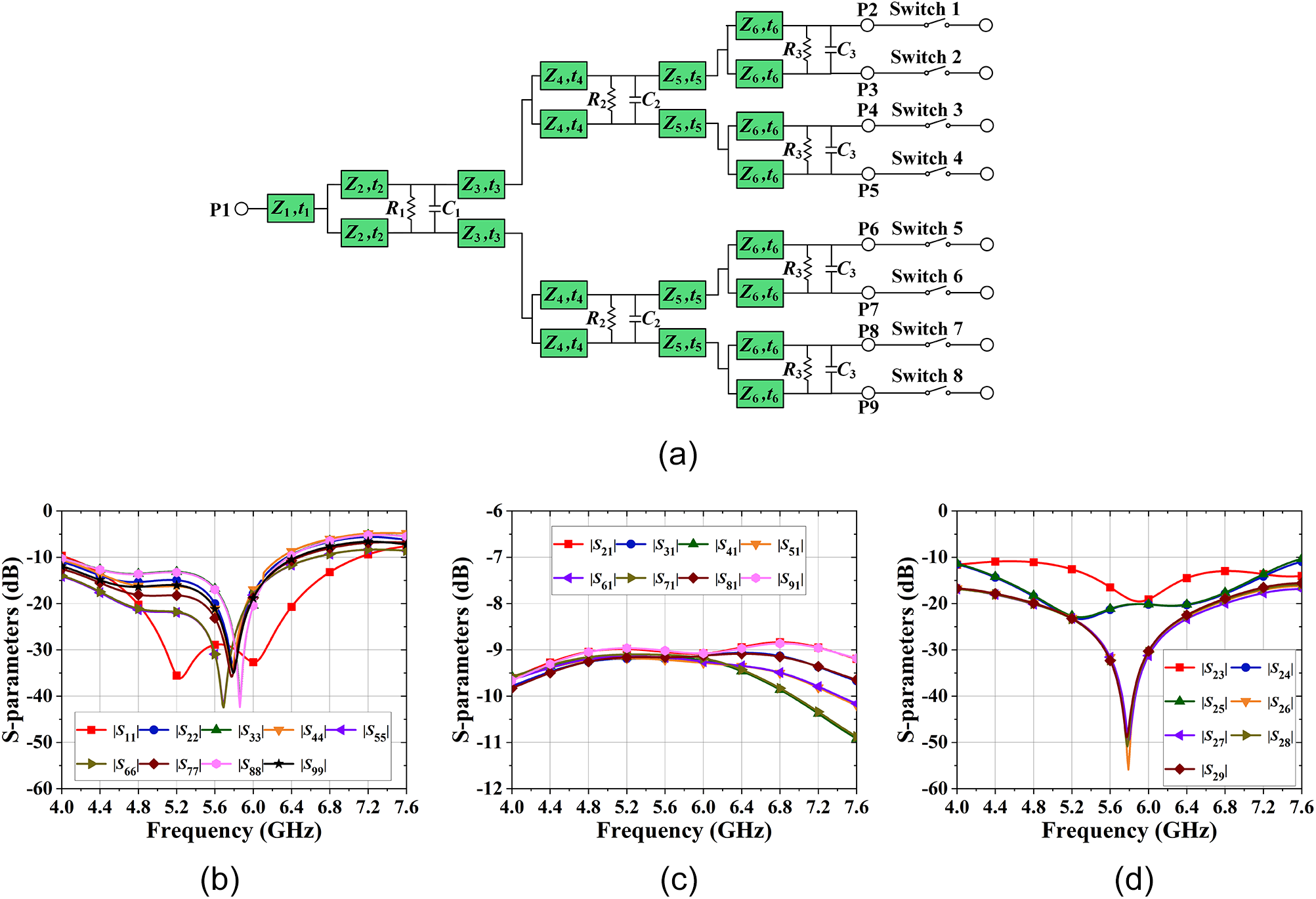
As shown in Fig. 3(a), the 1 × 8 switch control circuit consists of a compact eight-way equal power divider and eight switch circuits. For miniaturization, the RC-loaded Wilkinson power dividers in [Reference Deng and Chen20] are adopted for eight-way equal power distributions. Table 2 illustrates their theory parameters. Figure 3(b)–(d) show the simulated performances of the eight-way equal power divider. As can be seen in Fig. 3(b), in the frequency of 4.05–7.11 GHz, the simulated |S 11| is lower than −10 dB. For the output ports, the return losses are lower than −10 dB within the band of 4.05–6.29 GHz. Figure 3(c) shows that from 4.4 to 6.44 GHz, the loss for the output amplitude is lower than 0.5 dB. Within the working frequency band (5.5–6.1 GHz) of the matrix, the output amplitude loss is lower than 0.2 dB. Figure 3(d) gives the isolations of the power divider, where the 15-dB isolation bandwidth is 5.48–6.34 GHz.
Schematic and simulated performances of the 1 × 8 switch control circuit. (a) schematic. (b) return losses, (c) output amplitudes, and (d) isolations.

Theory parameters of the eight-way equal power divider

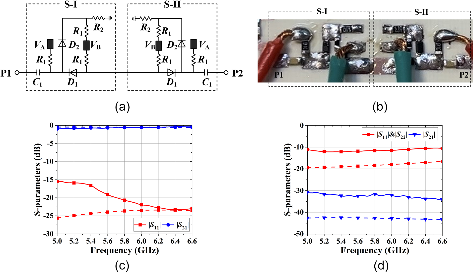
Since according to Table 1, two input ports of the arbitrary-amplitude 4 × 4 Matrix should be excited simultaneously, switch circuits connected to the output ports of the power divider are needed. As shown in Fig. 4(a), the switch circuit on each path is composed of two same sections, named as S-I and S-II. Here, the S-I is used for controlling the conduction and cutoff of the output from the power divider. While S-II is used for the on and off at input of the matrix. Among them, R 1 is the bias resistor and is equal to 10 kΩ, R 2 is served as the 50-Ω terminal load. C 1 = 1 nF is used for DC blocking. When V A < V B, the PIN diode D 1 conduct and the PIN diode D 2 cutoff, which corresponding to the ON state. On the contrary, the OFF state is realized. At OFF state, the terminal of the power divider and the 4 × 4 Matrix is connected to 50-Ω load. Figure 4(c) and (d) show the simulated and measured results of the switch at ON and OFF states, respectively. Here, the simulation is done by Ansoft HFSS, where the PIN diode part can not be simulated and is replaced by a connecting line. Thus, the simulation results are better than the measured results at both the ON and OFF state. In detail, at ON state, the simulated |S 11| is lower than −23.4 dB from 5.0 to 6.6 GHz and the loss is 0.5 dB. While the measured |S 11| is lower than −15.5 dB and the loss is 0.2–0.7 dB. At OFF state, the |S 11| and |S 22| almost coincide. The simulated |S 11| and |S 22| are lower than −16.5 dB from 5.0 to 6.6 GHz, and the isolation between the two ports is lower than −42.5 dB. While the measured |S 11| and |S 22| are lower than −10.5 dB and the isolation between the two ports is lower than −30.8 dB.
Picture and performance of one switch. (a) Layout, (b) photograph, (c) simulated (dash line with symbol) and measured (solid line with symbol) s-parameters at ON state, and (d) simulated (dash line with symbol) and measured (solid line with symbol) s-parameters at OFF state.

Implementation and measurements
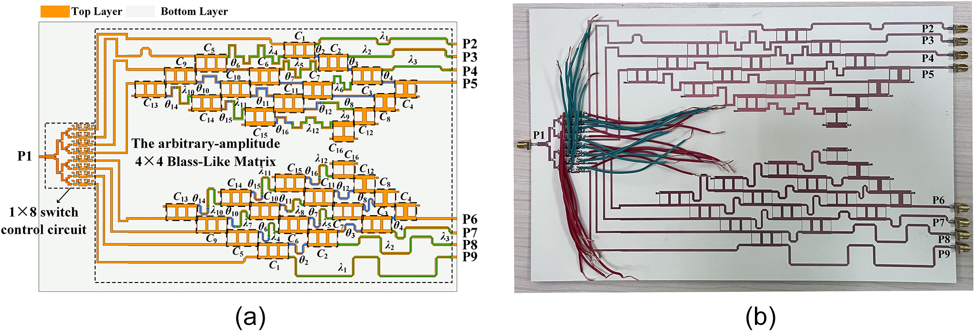
In this section, a prototype of the proposed Chebyshev-distributed beamforming network was designed and fabricated on a Rogers 4350B substrate (εr = 3.5, tan δ = 0.0037, h = 0.762 mm). Figure 5 shows the layout and photograph of the prototype. To achieve better flatness of the output amplitude, three-branch coupler is adopted for realizing the couplers in units A 4, A 8, A 12 and A 16, while four-branch coupler is used for other couplers. It is noted that for the three- and four-branch couplers, the values of α and β are 180°/270° and −90°/0°, respectively. Thus, by substituting the known values, such as the output Chebyshev distributions (0.143: 0.341: 0.71: 1: 1: 0.71: 0.341: 0.143), the output phase differences (−45°, 135°, 45° and −135°), and the coupler features, the values of coefficients ki for each coupler and phase for each phase shifter θi can be calculated according to (2)–(5). Table 3 shows the detailed values of ki and θi for each unit.
Layout (a) and photograph (b) of the proposed beamforming network.

Circuit parameters of the Chebyshev-distributed beamforming network

In addition, to ensure that the phase differences errors between the output ports of the beamforming network remains small within the operation band, the slope of the phase-frequency curve for all output ports needs to be consistent. However, due to that the proposed beamforming network is a serial network, the phase slopes at output ports show big differences, which results in large phase difference errors. To minimum the phase difference error and increase the phase bandwidth, phase compensation method is needed. In the design, simple transmission lines are added to each output ports for adjusting the phase slope. As shown in Fig. 5, λi is the electrical length of the transmission lines used for compensation, and their values are also listed in Table 3.
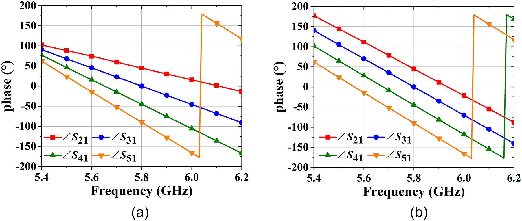
For better illustration, detailed compensation procedures for network M1 at state 1 are shown. As seen from Fig. 5(a), the numbers of couplers and phase shifters that the signal passes through are increased when output port numbers changes from 2 to 5. Thus, set the phase at port 5 as the reference, transmission lines are inserted to ports 4, 3, 2 in an order for compensation. Figure 6 plots the theory phase of ports 2–5 before and after compensation. It is observed from Fig. 6(a) that the phase slope of port 5 is different with ports 2, 3, and 4. To minimum the phase difference error between adjacent ports, different lengths of 50-Ω transmission lines are added for ports 2–4 to adjust the phase slopes. In addition, to ensure that the phase difference between output ports remains consistent after phase compensation, the electrical length of the compensation line λj is selected as 2nπ. As can be seen from Fig. 6(b), the phase slopes of the output phases are nearly parallel with each other after compensation.
The phase of ports 2–5 before and after compensation. (a) before compensation and (b) after compensation.

For the state 2, since the electrical lengths of the compensation lines λ 1, λ 2, and λ 3 are fixed, additional compensation lines with electrical length of 2nπ should be inserted to other signal paths, such as λ 4, λ 5, and λ 6. The compensation method is similar for states 3 and 4. Finally, by inserting several transmission lines, the in-band phase difference errors are reduced and the bandwidth is increased accordingly. Figure 7 gives the output port phase differences under different excitations with and without compensation. It is seen that before compensation, the bandwidths for 10° phase difference error are 2.7%, 3.4%, 2.9%, and 3.4% for the four states, while the values are increased to around 13.8%, 10.5%, 15.5%, and 10.3% after compensation.
Phase differences with (solid line) and without (dash line) compensation. (a) State 1, (b) state 2, (c) state 3, and (d) state 4.

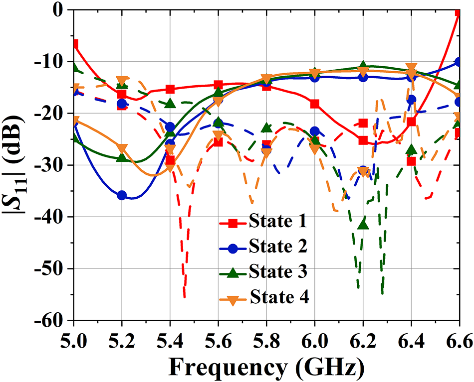
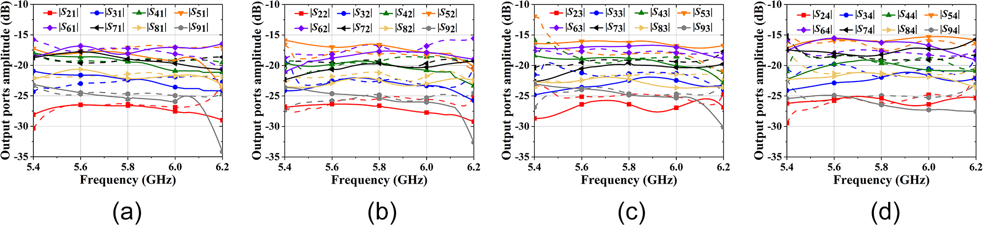
The Agilent N5230A is adopted in the measurement. Figure 8 plots the simulated and measured |S 11| of the designed prototype under four states according to Table 1. It is seen that an overlapped FBW of 24.1% (5.1–6.5 GHz) is obtained under the criterion of |S 11| < −10 dB for the four states. Figure 9 shows the output distributions at four states. It can be concluded that when the beamforming network is at state 1, the output port amplitudes at the center frequency are −26.60 dB, −22.35 dB, −19.40 dB, −18.11 dB, −18.08 dB, −18.94 dB, −22.15 dB, and −25.57 dB, respectively. Similarly, when the beamforming network is in the state 2, the output port amplitudes at the center frequency are −26.58 dB, −22.33 dB, −19.54 dB, −16.59 dB, −17.18 dB, −19.61 dB, −22.40 dB, and −25.36 dB. When the beamforming network is in the state 3 and 4, the output port amplitudes at the center frequency are −26.35 dB, −22.44 dB, −18.83 dB, −16.22 dB, −16.83 dB, −19.07 dB, −22.27 dB, −25.11 dB and −25.39 dB, −21.94 dB, −19.22 dB, −16.28 dB, −16.24 dB, −18.86 dB, −21.81 dB, −26.43 dB. Regardless of the state, the output amplitude follows the Chebyshev distribution and the measured errors are within ± 1 dB at the center frequency of 5.8 GHz. While for 1.5-dB amplitude imbalance, the measured FBWs at four states are 12.4%, 12.1%, 10.6%, and 10.3%, respectively.
Simulated (dash line with symbol) and measured (solid line with symbol) |S 11| of the prototype.

Simulated (dash line with symbol) and measured (solid line with symbol) output ports amplitudes. (a) State 1, (b) State 2, (c) State 3, and (d) state 4.

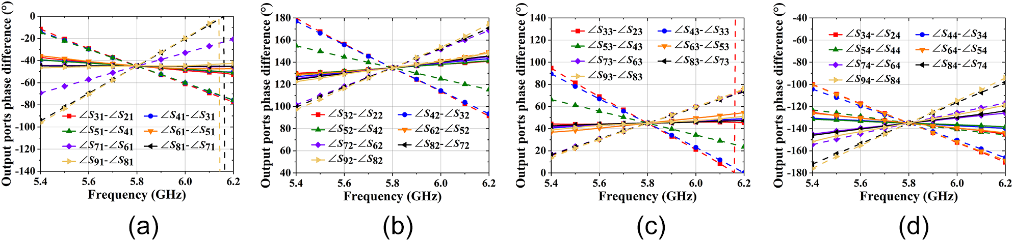
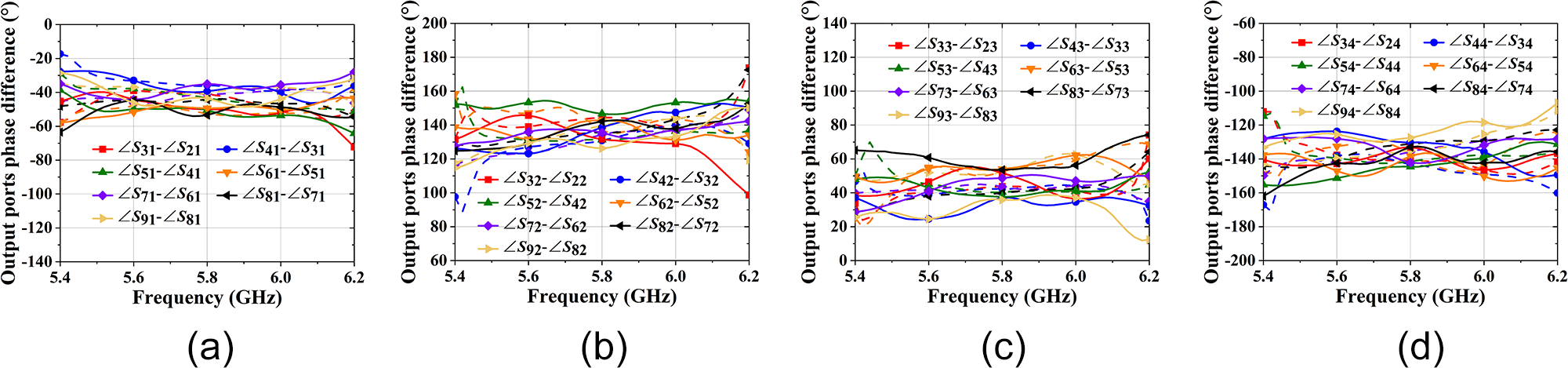
The output ports phase differences of the designed Chebyshev-distributed beamforming network are shown in Fig. 10. At state 1, the phase differences between output ports are −49°, −39°, −50°, −49°, −35°, −53°, and −43° at the center frequency. While at state 2, the corresponding values are 131°, 138°, 145°, 142°, 135°, 142°, and 126°. The phase differences at state 3 and 4 are 51°, 37°, 37°, 54°, 48°, 53°, 35°, and −133°, −130°, −144°, −138°, −142°, −133°, −127°, respectively. As seen in Fig. 10, both the measurement and simulation results are within ± 10° at the center frequency. Under the standard of 15° phase error, the bandwidths are 14.1%, 11.3%, 13.1%, and 10.3%, respectively.
Simulated (dash line with symbol) and measured (solid line with symbol) output ports phase difference. (a) State 1, (b) state 2, (c) state 3, and (d) state 4.

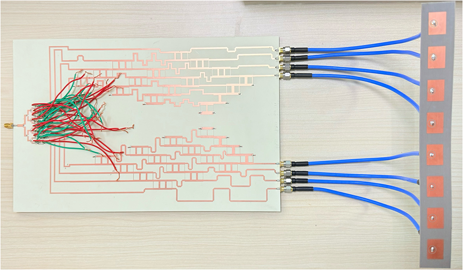
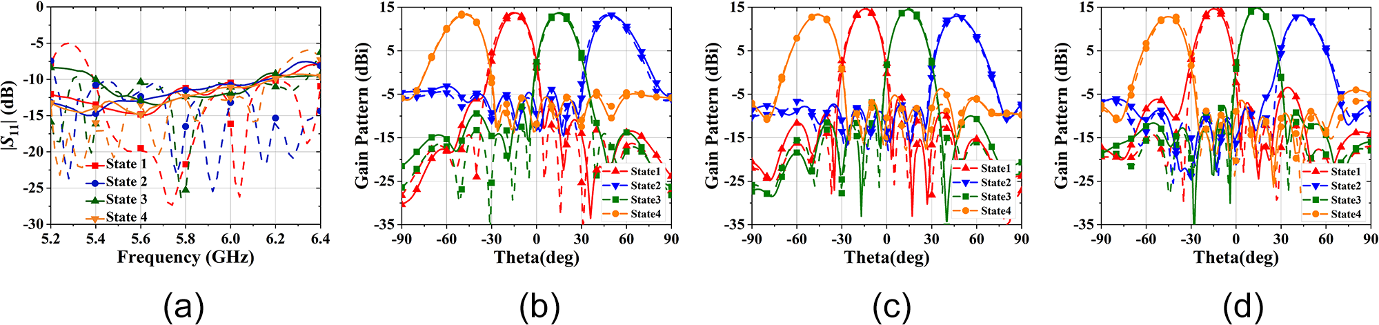
Finally, the designed prototype is connected to a 1 × 8 patch array, as shown in Fig. 11. The size of the 1 × 8 patch array is 215.7 mm × 26.5 mm, yielding 4.15 λg × 0.51 λg (λg is the free-space wavelength at the 5.8 GHz). Figure 12(a) shows the simulated and measured |S 11| of the 1 × 8 patch array excited by the proposed network. As observed, both the simulated and measured |S 11| are lower than − 10 dB over the designed frequency range of 5.42–6.14 GHz. Figure 12(b)–(d) depict the simulated and measured gain patterns at 5.5 GHz, 5.8 GHz, and 6.1 GHz. It is observed from the measured results that by switching the control circuit, four beams pointing at the angles of − 15°, 45°, 15°, −45° are realized at the three frequencies. At the center frequency of 5.8 GHz, the realized gains for four states are 14.6 dBi, 12.9 dBi, 14.4 dBi, 13.2 dBi, and the SLLs are −20.2 dB, −20.3 dB, − 21.1dB, −20.9 dB, respectively. At the frequency of 5.5 GHz, the realized gains are 13.7 dBi, 12.7 dBi, 13.6 dBi, 13.1 dBi, and the SLLs are −20.6 dB, −21.6 dB, −21.7 dB, and −20.9 dB. In addition, the realized gains are 14.6 dBi, 13.0 dBi, 14.8 dBi, 12.8 dBi and the SLLs are −22.4 dB, −20.1 dB, −20.7 dB, −20.0 dB at 6.1 GHz. The measured realized gains vary from 12.7 to 14.8 dBi.
Photograph of the multi-beam antenna with the proposed network.

Simulated (dash line with symbol) and measured (solid line with symbol) results. (a) |S 11|, (b) gain patterns at 5.5 GHz, (c) gain patterns at 5.8 GHz, and(d) gain radiation patterns at 6.1 GHz.

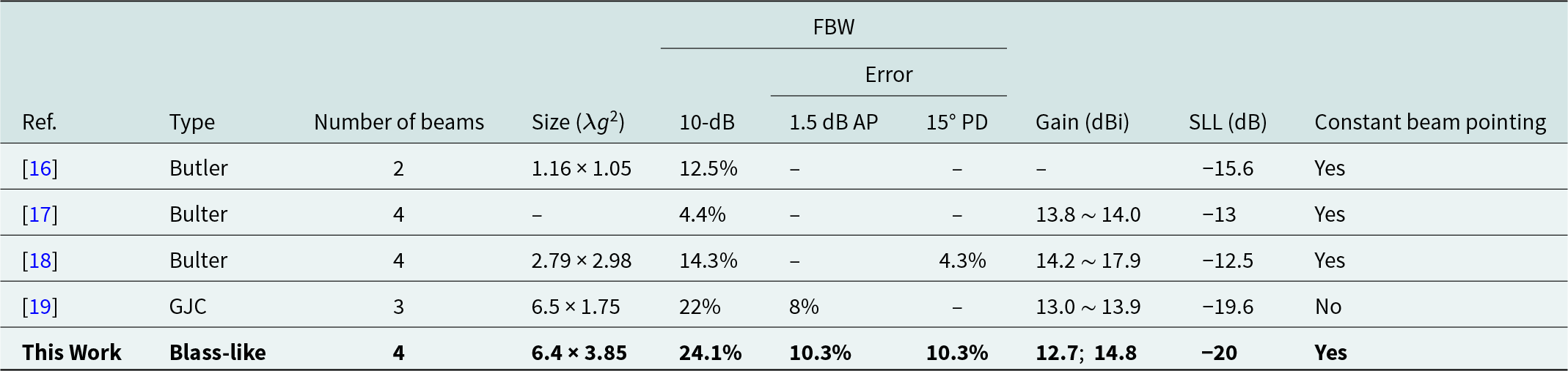
Table 4 compares the proposed Chebyshev-distributed beamforming network with other representative beamforming networks. It is found that the proposed beamforming network exhibits the largest bandwidth under 10-dB return loss, 1.5-dB AP imbalance, and 15° PD. Moreover, the SLL of the proposed design is the smallest and the beam pointing is constant, which demonstrates its potential applications in multi-beam antennas for precise receiving and improved anti-interference performance.
Comparisons between the proposed and reported beamforming networks

λg is the free-space wavelength at the center frequency. FBW: Fractional bandwidth, SLL: sidelobe level, AP: Amplitude distribution, PD: Phase Difference.
Conclusion
A Chebyshev-distributed beamforming network composed of two arbitrary-amplitude 4 × 4 Blass-like matrices and one 1 × 8 switch control circuit is demonstrated in the paper, which can be used for generating four beams with low sidelobes. Besides, phase compensation method is applied for obtaining minimum phase difference errors in the operated bandwidth. Measurement results indicate that the network show a 10-dB impedance bandwidth of 24.1%. Under the criterion of 1.5-dB amplitude imbalance and 15° phase difference error, the bandwidth reaches 10.3%. Due to that the proposed network has the advantages of flexible control of beamforming, tapered amplitude distribution, and balanced phase performance, it has potential application prospects in multi-beam antennas for precise receiving and improved anti-interference performance.
Acknowledgment
This work was supported in part by the National Natural Science Foundation of China under Grant 52471371, in part by the Young Elite Scientists Sponsorship Program by CAST under Grant 2022QNRC001, and in part by the China Scholarship Council under Grant 202406570025.
Competing interests
The authors report no conflict of interest.
Appendix
 \begin{align}\left\{ {\begin{array}{*{20}{l}}
{{S_{51}} = {S_{1\_21}}} \\
{{S_{61}} = {S_{1\_31}}{S_{2\_21}}} \\
{{S_{71}} = {S_{1\_31}}{S_{2\_31}}{S_{3\_21}}} \\
{{S_{81}} = {S_{1\_31}}{S_{2\_31}}{S_{3\_31}}{S_{4\_21}}}
\end{array}} \right.\end{align}
 \begin{align}\left\{ {\begin{array}{*{20}{l}}
{{S_{52}} = {S_{5\_21}}{S_{1\_24}}} \\
{{S_{62}} = {S_{5\_21}}{S_{1\_34}}{S_{2\_21}} + {S_{5\_31}}{S_{6\_21}}{S_{2\_24}}} \\
{{S_{72}} = {S_{5\_21}}{S_{1\_34}}{S_{2\_31}}{S_{3\_21}} + {S_{5\_31}}{S_{6\_21}}{S_{2\_34}}{S_{3\_21}} + {S_{5\_31}}{S_{6\_31}}{S_{7\_21}}{S_{3\_24}}} \\
{{S_{82}} = \left( \begin{aligned}
& {S_{5\_21}}{S_{1\_34}}{S_{2\_31}}{S_{3\_31}}{S_{4\_21}} + {S_{5\_31}}{S_{6\_21}}{S_{2\_34}}{S_{3\_31}}{S_{4\_21}} \\
& + {S_{5\_31}}{S_{6\_31}}{S_{7\_21}}{S_{3\_34}}{S_{4\_21}} + {S_{5\_31}}{S_{6\_31}}{S_{7\_31}}{S_{8\_21}}{S_{4\_34}} \end{aligned} \right)}
\end{array}} \right.\end{align}
 \begin{align}\left\{ {\begin{array}{*{20}{l}}
{{S_{53}} = {S_{9\_21}}{S_{5\_24}}{S_{1\_24}}} \\
{{S_{63}} = {S_{9\_21}}{S_{5\_24}}{S_{1\_34}}{S_{2\_21}} + {S_{9\_21}}{S_{5\_34}}{S_{6\_21}}{S_{2\_24}} + {S_{9\_31}}{S_{10\_21}}{S_{6\_24}}{S_{2\_24}}} \\
{{S_{73}} = \left( \begin{aligned}
& {S_{9\_21}}{S_{5\_24}}{S_{1\_34}}{S_{2\_31}}{S_{3\_21}} + {S_{9\_21}}{S_{5\_34}}{S_{6\_21}}{S_{2\_34}}{S_{3\_21}} \\
& + {S_{9\_21}}{S_{5\_34}}{S_{6\_31}}{S_{7\_21}}{S_{3\_24}} + {S_{9\_31}}{S_{10\_21}}{S_{6\_24}}{S_{2\_34}}{S_{3\_21}} \\
& + {S_{9\_31}}{S_{10\_21}}{S_{6\_34}}{S_{7\_21}}{S_{3\_24}} + {S_{9\_31}}{S_{10\_31}}{S_{11\_21}}{S_{7\_34}}{S_{3\_24}} \end{aligned} \right)} \\
{{S_{83}} = \left( \begin{aligned}
& {S_{9\_21}}{S_{5\_24}}{S_{1\_34}}{S_{2\_31}}{S_{3\_31}}{S_{4\_21}} + {S_{9\_21}}{S_{5\_34}}{S_{6\_21}}{S_{2\_34}}{S_{3\_31}}{S_{4\_21}} \\
& + {S_{9\_21}}{S_{5\_34}}{S_{6\_31}}{S_{7\_21}}{S_{3\_34}}{S_{4\_21}} + {S_{9\_21}}{S_{5\_34}}{S_{6\_31}}{S_{7\_31}}{S_{8\_21}}{S_{4\_24}} \\
& + {S_{9\_31}}{S_{10\_21}}{S_{6\_24}}{S_{2\_34}}{S_{3\_31}}{S_{4\_21}} + {S_{9\_31}}{S_{10\_21}}{S_{6\_34}}{S_{7\_21}}{S_{3\_34}}{S_{4\_21}} \\
& + {S_{9\_31}}{S_{10\_21}}{S_{6\_34}}{S_{7\_34}}{S_{8\_21}}{S_{4\_24}} + {S_{9\_31}}{S_{10\_31}}{S_{11\_21}}{S_{7\_24}}{S_{3\_34}}{S_{4\_21}} \\
& + {S_{9\_31}}{S_{10\_31}}{S_{11\_21}}{S_{7\_34}}{S_{8\_21}}{S_{4\_24}} + {S_{9\_31}}{S_{10\_31}}{S_{11\_31}}{S_{12\_21}}{S_{8\_24}}{S_{4\_24}} \end{aligned} \right)}
\end{array}} \right.\end{align}
 \begin{align}\left\{ {\begin{array}{*{20}{l}}
{{S_{54}} = {S_{13\_21}}{S_{9\_24}}{S_{5\_24}}{S_{1\_24}}} \\
{{S_{64}} = \left( \begin{aligned}
& {S_{13\_21}}{S_{9\_24}}{S_{5\_24}}{S_{1\_34}}{S_{2\_21}} + {S_{13\_21}}{S_{9\_24}}{S_{5\_34}}{S_{6\_21}}{S_{2\_24}} \\
& + {S_{13\_21}}{S_{9\_43}}{S_{10\_21}}{S_{6\_24}}{S_{2\_24}} + {S_{13\_31}}{S_{14\_21}}{S_{10\_24}}{S_{6\_24}}{S_{2\_24}} \end{aligned} \right)} \\
{{S_{74}} = \left( \begin{aligned}
& {S_{13\_21}}{S_{9\_24}}{S_{5\_24}}{S_{1\_34}}{S_{2\_31}}{S_{3\_21}} + {S_{13\_21}}{S_{9\_24}}{S_{5\_34}}{S_{6\_21}}{S_{2\_34}}{S_{3\_21}} \\
& + {S_{13\_21}}{S_{9\_24}}{S_{5\_34}}{S_{6\_31}}{S_{7\_21}}{S_{3\_24}} + {S_{13\_21}}{S_{9\_34}}{S_{10\_21}}{S_{6\_24}}{S_{2\_34}}{S_{3\_21}} \\
& + {S_{13\_21}}{S_{9\_34}}{S_{10\_21}}{S_{6\_34}}{S_{7\_12}}{S_{3\_24}} + {S_{13\_21}}{S_{9\_34}}{S_{10\_31}}{S_{11\_21}}{S_{7\_24}}{S_{3\_24}} \\
& + {S_{13\_31}}{S_{14\_21}}{S_{10\_24}}{S_{6\_24}}{S_{2\_34}}{S_{3\_21}} + {S_{13\_31}}{S_{14\_21}}{S_{10\_24}}{S_{6\_34}}{S_{7\_21}}{S_{3\_24}} \\
& + {S_{13\_31}}{S_{14\_21}}{S_{10\_34}}{S_{11\_21}}{S_{7\_24}}{S_{3\_24}} + {S_{13\_31}}{S_{14\_31}}{S_{15\_21}}{S_{11\_24}}{S_{7\_24}}{S_{3\_24}} \end{aligned} \right)} \\
{S_{84}} = \left( \begin{aligned}
& {S_{13\_21}}{S_{9\_24}}{S_{5\_24}}{S_{1\_34}}{S_{2\_31}}{S_{3\_31}}{S_{4\_21}} + {S_{13\_21}}{S_{9\_24}}{S_{5\_34}}{S_{6\_21}}{S_{2\_34}}{S_{3\_31}}{S_{4\_21}} \\
& + {S_{13\_21}}{S_{9\_24}}{S_{5\_34}}{S_{6\_31}}{S_{7\_21}}{S_{3\_34}}{S_{4\_21}} + {S_{13\_21}}{S_{9\_24}}{S_{5\_34}}{S_{6\_31}}{S_{7\_31}}{S_{8\_21}}{S_{4\_24}} \\
& + {S_{13\_21}}{S_{9\_34}}{S_{10\_21}}{S_{6\_24}}{S_{2\_34}}{S_{3\_31}}{S_{4\_21}} + {S_{13\_21}}{S_{9\_34}}{S_{10\_21}}{S_{6\_34}}{S_{7\_21}}{S_{3\_34}}{S_{4\_21}} \\
& + {S_{13\_21}}{S_{9\_34}}{S_{10\_21}}{S_{6\_34}}{S_{7\_31}}{S_{8\_21}}{S_{4\_24}} + {S_{13\_21}}{S_{9\_34}}{S_{10\_31}}{S_{11\_21}}{S_{7\_24}}{S_{3\_34}}{S_{4\_21}} \\
& + {S_{13\_21}}{S_{9\_34}}{S_{10\_31}}{S_{11\_21}}{S_{7\_34}}{S_{8\_21}}{S_{4\_24}} + {S_{13\_21}}{S_{9\_34}}{S_{10\_31}}{S_{11\_31}}{S_{12\_21}}{S_{8\_24}}{S_{4\_24}} \\
& + {S_{13\_21}}{S_{14\_21}}{S_{10\_24}}{S_{6\_24}}{S_{2\_34}}{S_{3\_31}}{S_{4\_21}} + {S_{13\_21}}{S_{14\_21}}{S_{10\_24}}{S_{6\_34}}{S_{7\_21}}{S_{3\_34}}{S_{4\_21}} \\
& + {S_{13\_21}}{S_{14\_21}}{S_{10\_24}}{S_{6\_34}}{S_{7\_31}}{S_{8\_21}}{S_{4\_24}} + {S_{13\_21}}{S_{14\_21}}{S_{10\_34}}{S_{11\_21}}{S_{7\_24}}{S_{3\_34}}{S_{4\_21}} \\
& + {S_{13\_21}}{S_{14\_21}}{S_{10\_34}}{S_{11\_21}}{S_{7\_34}}{S_{8\_21}}{S_{4\_24}} + {S_{13\_21}}{S_{14\_21}}{S_{10\_34}}{S_{11\_31}}{S_{12\_21}}{S_{8\_24}}{S_{4\_24}} \\
& + {S_{13\_21}}{S_{14\_31}}{S_{15\_21}}{S_{11\_24}}{S_{7\_24}}{S_{3\_34}}{S_{4\_21}} + {S_{13\_21}}{S_{14\_31}}{S_{15\_21}}{S_{11\_24}}{S_{7\_34}}{S_{8\_21}}{S_{4\_24}} \\
& + {S_{13\_21}}{S_{14\_31}}{S_{15\_21}}{S_{11\_34}}{S_{12\_21}}{S_{8\_24}}{S_{4\_24}} + {S_{13\_21}}{S_{14\_31}}{S_{15\_31}}{S_{16\_21}}{S_{12\_24}}{S_{8\_24}}{S_{4\_24}} \end{aligned} \right)
\end{array}} \right.\end{align}

Shuo Li was born in Hebei, China. She received the B.S. degree in information engineering from East China Jiaotong University (ECJTU), Jiangxi, China, in 2022. She is currently working toward the Ph.D degree at Dalian Maritime University. Her current research interests include the beamforming networks and reconfigurable devices.

Hongmei liu (Member, IEEE) received the Ph.D. degree in information and communication engineering from Dalian Maritime University (DMU), China, in 2016. She is currently a Full Professor with the School of Information Science and Technology, DMU. Her current research interests include multi-beam antenna, beamforming networks, CP antennas, multi-function microwave circuits, and reconfigurable RF components. She has authored or co-authored over 90 papers in journals and conferences. She is currently serving as a Technical Reviewer for the IEEE Transactions on Microwave Theory and Techniques, IEEE Transactions on Circuits and Systems, IEEE Transactions on Industrial Electronics, IEEE Microwave and Wireless Components Letters, IET Microwaves, Antennas & Propagation, Electronics Letters, International Journal of RF and Microwave Computer-Aided Engineering, and AEU-International Journal of Electronics and Communications. She was a recipient of the Best Doctor’s Dissertation Award of Liaoning Province in 2017.

Yan Zhang was born in Shanxi, China. She received the B.S. degree in communication engineering from Dalian Jiaotong University (DJTU), China, in 2018, and the Master degree in electronic and communication engineering from Dalian Maritime University (DMU), China, in 2021. She is currently pursuing the Ph.D degree at DMU. Her research interests include filtering couplers and beamforming networks.

Zhongbao wang (Member, IEEE) received the Ph.D. degree in communication and information systems from Dalian Maritime University (DMU), China, in 2012. He is currently a Full Professor with the School of Information Science and Technology, DMU. From 2014 to 2018, he was a Postdoctoral Fellow with Beijing University of Posts and Telecommunications. From 2019 to 2020, he is a Visiting Scholar with the Department of Electrical and Computer Engineering, National University of Singapore, Singapore. His current research interests include passive RF components, patch antennas, and microwave technology using artificial intelligence. He has authored or co-authored two books and over 90 papers in journals and conferences. He is currently serving as a Technical Reviewer for journals such as the IEEE Transactions on Microwave Theory and Techniques, IEEE Transactions on Circuits and Systems, IEEE Transactions on Industrial Electronics, IEEE Microwave and Wireless Components Letters, IEEE Antennas and Wireless Propagation Letters and IEEE Access. He was a recipient of the Best Doctor’s Dissertation Award of Liaoning Province in 2013.