Expected Utility

The first approach involves expected utility theory, which Shepsle (Reference Shepsle1972) and nearly all subsequent contributors have used to analyze choices between precise and ambiguous candidates. In this framework, each voter evaluates candidates based on the satisfaction candidates are likely to bring. The expected utility from candidate P is simply EU(P) = u(p), where p represents the candidate's position and u(.) is the voter's utility function. The anticipated payoff from A is slightly more complicated because the voter cannot know in advance which outcome A will produce. The expected outcome from electing A is a probability-weighted average, E(A) ≡ μ = ∫_aaf(a)da, where f(a) gives the probability density of each position a that the ambiguous candidate could take. Similarly, the expected utility from selecting the ambiguous candidate is EU(A) = ∫_au(a)f(a)da.

Whether the expected utility criterion favors the ambiguous candidate depends partly on the voter's attitude toward risk, as reflected in the shape of u(.). Researchers commonly assume that voters are risk averse (Alvarez Reference Alvarez1998; Bartels Reference Bartels1986; Enelow and Hinich Reference Enelow and Hinich1981; Gill Reference Gill2005) (i.e., they receive less utility from playing the lottery than from receiving its expected payoff with certainty, such that EU(A) < u(μ)). Risk-averse voters would prefer the precise candidate whenever p = μ, and they might opt for the precise candidate even when the ambiguous one is closer (when |v − μ| < |v − p|, where v is the voter's ideal point), to avoid the risk that the ambiguous candidate could deliver an undesirable outcome.

What if some voters are risk acceptant, and thus prefer gambles over their expected outcomes, such that EU(A) > u(μ)? Shepsle (Reference Shepsle1972) analyzes the implications of risk acceptance when an incumbent candidate, whose position is known with certainty, confronts a challenger who can pursue a strategy of ambiguity. If the incumbent were located at p, the challenger could win the support of risk-acceptant voters by adopting an ambiguous platform with mean value μ = p. Moreover, even if v were closer to p than to μ, risk-acceptant voters might gamble on A in the hope of getting a favorable outcome. Shepsle's analysis identifies one reason why voters might prefer ambiguous candidates over precise alternatives.Footnote ³

An important exception arises when the precise candidate advocates a policy on the voter's ideal point. In this situation and others like it, even risk-acceptant voters (those with convex loss functions) would prefer the precise candidate. After all, when the precise candidate and the voter coincide, the voter cannot gain and may in fact lose by selecting the risky candidate (Bendor and Meirowitz Reference Bendor and Meirowitz2004, 297; Page Reference Page1976, 747). Our empirical analysis, discussed later, exploits this fact to show why risk acceptance cannot explain the behavior of some participants in our experiments.

Biased Probabilities

To this point, we have assumed that people use objective probabilities: they soberly evaluate where candidates are likely to stand, given the available information. We now relax this assumption and explore the possibility that voters have biased perceptions about the policies that ambiguous candidates actually favor.

The first possibility is general optimism: when confronted with an ambiguous candidate, optimistic voters assume the candidate is closer to themselves than the facts warrant. Operationally, they perceive a probability distribution more favorable to themselves than the evidence implies, resulting an expectation μ_I such that |v − μ_I| < |v − μ|. This optimistic misperception, if present, should increase the likelihood that the voter would choose the ambiguous candidate over the precise one.

Previous research suggests the plausibility of this hypothesis. Psychological studies since the 1950s, for example, have documented that people systematically overestimate the probability of desirable events (e.g., Irwin Reference Irwin1953; Rosenhan and Messick Reference Rosenhan and Messick1966). Studies have also uncovered powerful evidence of a “false consensus effect,” in which people overestimate the probability of agreement with others whose views are not already known. Importantly, people tend to make this mistake “regardless of their sentiment toward the group” (Krosnick Reference Krosnick and Kuklinski2002, 125). Across-the-board optimism should give ambiguous candidates a boost in competition against precise candidates.

An alternative hypothesis holds that voters are selectively optimistic and pessimistic; they expand or contract the perceived distance between themselves and an ambiguous candidate, depending on the degree of affective affinity for the candidate (Bartels Reference Bartels1988, 98–101). This idea is the focus of an extensive but currently inconclusive literature about how citizens project views onto candidates (Krosnick Reference Krosnick and Kuklinski2002). Democratic voters, for example, might exhibit positive (proximity-enhancing) bias toward Democrats but negative (proximity-detracting) bias toward Republicans. When courting Democratic voters, then, ambiguity could aid Democratic candidates but undermine Republican ones.

Other Conditions That Favor Ambiguous Candidates

These theories do not exhaust the set of interesting possibilities. One could model utility not only as a function of the distance between the voter and the candidate, but also as a function of candidate traits that do not fit conveniently into the standard spatial framework. For example, voters in a complex world might value flexibility—a willingness to adapt to changing circumstances instead of clinging to singular positions. Candidates who take broad stands in campaigns may signal their flexibility and therefore score points in the eyes of some voters, especially ones who are not rigid about their own positions.Footnote ⁴

Alternatively, ambiguity could evoke a negative reaction, even among voters who might otherwise sympathize with the range of positions in a candidate's platform. As Campbell (Reference Campbell1983, 278) conjectures, ambiguity could “hurt a candidate's public image” by revealing the candidate as “evasive or spineless.” Thus, ambiguity could be consequential not only because it affects the assumed positions of candidates, but also because it informs judgments about candidates' character.

Problems of Measurement

The American National Election Study (NES) took a valuable step toward measuring candidate issue stances when it began asking respondents to locate candidates on seven-point issue scales. Unfortunately, most NES surveys do not directly measure individual perceptions about the precision of candidate platforms. Participants assign each candidate to a single point, usually without indicating how certain they feel or whether the candidate might stand elsewhere (Weisberg and Fiorina Reference Weisberg, Fiorina, Pierce and Sullivan1980).

Recognizing this problem, scholars have devoted much creative energy to developing indirect proxies for uncertainty about candidate positions. Bartels (Reference Bartels1986) proposed one approach, based on the pattern of “don't know” responses. Suppose that each person has a latent degree of uncertainty about where the candidate stands; that people whose uncertainty exceeds a particular threshold refuse to place the candidate on the scale; and that uncertainty, although unobservable, varies with demographic and contextual variables that are present in the NES. One could then estimate a probit model of nonresponse, compute the predicted probability of nonresponse for each citizen with respect to each candidate and issue, and use the predicted probabilities as measures of uncertainty.

Even proponents of the probit method acknowledge, however, that it “requires strong assumptions” (Berinsky and Lewis Reference Berinsky and Lewis2007, 144) and is “sufficiently indirect that any attempt to derive general conclusions about the political significance of issue uncertainty would be foolhardy” (Bartels Reference Bartels1986, 726). Indeed, the two leading applications of this approach have reached opposite conclusions about the effects of uncertainty (Bartels Reference Bartels1986; Berinsky and Lewis Reference Berinsky and Lewis2007).

Other scholars have used the sample distribution of issue placements as a measure of uncertainty. Campbell (Reference Campbell1983) computed the standard deviation of public perceptions about each candidate's position, and Gill (Reference Gill2005) calculated entropy scores. As Bartels (Reference Bartels1986, 710) pointed out, however, there is no necessary connection between individual-level uncertainty and populationwide variability. If, for example, all voters were uncertain about a candidate's position but had exactly the same expectation, standard deviations and entropy scores would overstate voters' certainty. Conversely, if voters disagreed about where a candidate stood but were completely firm in their beliefs, standard deviations and entropy scores would overstate the uncertainty in voters' minds.

A few scholars have directly measured people's certainty about candidate positions. In a unique study, Alvarez and Franklin (Reference Alvarez and Franklin1994) not only asked respondents to locate candidates on a scale, but also invited them to say whether they were “very certain, pretty certain, or not very certain” about where each candidate stood (also see NES 1994 and 1996). Brady and Ansolabehere (Reference Brady and Ansolabehere1989) employed a related procedure by treating each person's self-reported knowledge about a candidate as an index of their awareness of the candidate's position. Subjective measures of certainty hold much promise, but they are rarely available in standard surveys, and they leave open the question of whether point estimates reflect the mean, the mode, the worst case, the best case, or a random draw from the candidate's probability distribution.

Moreover, none of these measures isolates the actual ambiguity in candidate position statements. Instead, each quantifies the total uncertainty arising from numerous sources, only one of which is the vagueness of candidate proclamations. Consequently, one cannot infer how much of the reaction is due to candidate vagueness versus other sources of uncertainty.

Problems of Endogeneity

Even without measurement problems, three sources of endogeneity make inference difficult. First, candidates are strategic: they take into account the likely reaction of voters when deciding how much information to reveal. Rational candidates avoid making vague statements to audiences who would react harshly against it, and they avoid speaking precisely when specificity would damage their electoral fortunes. Thus, the strategic behavior of candidates confounds efforts by researchers to detect the consequences of ambiguity.

Second, voters are more attentive to candidates they like. People initially drawn to a candidate's charisma, race, or experience, for example, may end up attending rallies and following media reports about the candidate, and thereby learning about the candidate's policy positions. Election primaries reinforce this pattern. Registered Democrats, for example, are especially likely to participate in Democratic primaries. They follow Democratic candidates throughout the primary season and accumulate information about their platforms. By the time the general election campaign begins, Democratic voters will know more about their party's candidate than about the opposition. Thus, both psychological and institutional forces lead citizens to learn about the issue positions of candidates they already favor for other reasons. Unless somehow controlled, this endogeneity will cause researchers to overstate the costs of ambiguity.

Finally, voters may overestimate the precision of positions articulated by candidates they like. Ambiguity gives voters leeway to see what they want: to perceive a candidate as being similar to themselves. If citizens encounter a candidate who seems attractive on other grounds, they may perceive more of the candidate's probability distribution as being piled near their own ideal point. In the extreme, voters may perceive the candidate as a probability spike over the most attractive point in the candidate's range. When asked about the candidate's level of ambiguity, voters may then report more precision than the facts warrant. In the minds of voters—and therefore the data sets of researchers—the vague candidate will appear artificially precise, causing a downward bias in the estimated benefits of ambiguity.

Taken together, problems of measurement and endogeneity pose seemingly insurmountable obstacles to studying the effects of candidate ambiguity. In the next section, we describe an experiment that overcomes these obstacles.

Measuring Respondents' Ideal Points

The survey began by asking respondents about a key political issue, government provision of services. Following the NES, we explained: “Some people think the government should provide fewer services even in areas such as health and education in order to reduce spending. Other people feel it is important for the government to provide many more services, even if it means an increase in spending.” We then asked respondents to select one of seven alternatives: increase services by a large, medium, or small amount; keep the same amount of services; or decrease services by a small, medium, or large amount. The positions were described verbally rather than numerically, though for convenience we sometimes use the integers one through seven as shorthand for the seven fully labeled options.

As a follow-up, we asked half the participants how certain they were about their own position. The options included extremely sure, very sure, moderately sure, slightly sure, and not sure at all. We assigned this question to only half the sample to guard against the possibility of priming. Respondents who expressed certainty about their own position, for example, might have felt pressure to choose precise candidates over vague ones with similar expected locations, in order to remain consistent with their stated level of certainty. As it turned out, our concerns about priming were unwarranted: respondents behaved similarly regardless of whether they had been asked about the firmness of their own position.

Measuring Preferences about Candidates

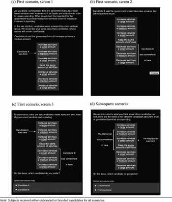
We then asked respondents to choose between two candidates, one vague and the other precise. “In the last election,” participants were told, “candidates were surveyed by a non-partisan group. We would like your views about two candidates, whose names will remain confidential.” Using the same issue and policy options that respondents had seen previously, we offered verbal and graphical summaries of the platforms of two candidates (Figure 1a–c). The precise candidate took one of seven discrete positions on the scale. The ambiguous candidate, in contrast, advocated that “the government should increase services” or that “the government should decrease services,” but in neither case said how much. Our description of the vague candidate was purposefully neutral. We avoided language that might have been taken as criticism or praise of ambiguity. After displaying the views of both candidates, we asked who the respondent preferred on that issue.Footnote ⁵

FIGURE 1.

Measuring Preferences for Precise versus Ambiguous Candidates

Half the respondents encountered unbranded candidates, who were identified by letters such as “A” and “B”; the other half encountered party branded candidates, who were labeled as Democrat and Republican. Each type offered unique opportunities for inference. By denoting some candidates with letters, we were able to test many theories of ambiguity in their purest form, without the potentially confounding effects of party. By denoting other candidates as Democrat and Republican, the design allowed us to study how partisanship—one of the most powerful factors in electoral politics—conditions the consequences of ambiguity.Footnote ⁶ Respondents retained their initial assignments (unbranded or branded) for the duration of the interview.

We also randomized the locations of candidates. Our stratified random assignment algorithm ensured, to the greatest extent possible, that each respondent had an equal chance of receiving one of four types of scenarios. In Type I, the precise candidate was closer to the voter (i.e., |v − p| < |v − μ|, where v was the voter's bliss point, p was the position of the precise candidate, and μ was the center of the vague candidate's interval). Type II reversed the inequality, such that the ambiguous candidate was the proximity favorite. Type III, a straddle tie, occurred when the precise candidate took a position at the center of the vague candidate's interval (i.e., p = μ). Finally, Type IV, a reflected tie, arose when the respondent stood between the two candidates and was equidistant to them (i.e., p ≠ μ and |v − p| = |v− μ|).Footnote ⁷

Having asked about one pair of candidates, we invited respondents to consider another: “We are interested in what you think about other candidates, as well. Here are the views of two different candidates about the level of government services and spending.” Once again, the precise candidate was randomly assigned to one of the seven discrete positions. The ambiguous candidate, in contrast, took one of the three central ranges: increase medium to keep the same, increase small to decrease small, or keep the same to decrease medium. Because these positions were more cumbersome to describe verbally, we leveraged respondents' familiarity with our format by offering a graphical summary without a verbal description, as in Figure 1d.Footnote ⁸

We ended this phase of the experiment by displaying two more pairs of candidates, some of which we positioned to allow within-subject analysis of the effects of ambiguity. Our method involved mimicking the earlier scenarios but, in each case, replacing the ambiguous candidate with a precise candidate who stood at the midpoint of the previous ambiguous interval. We presented these “precise scenarios” as if they involved entirely new candidates, rather than ones that respondents had already encountered.Footnote ⁹ By studying the choices each voter made in the ambiguous scenario and its matching precise scenario, we inferred the voter's response to changes in candidate ambiguity, holding other factors constant.

Measuring Expectations and Taste for Risk

The third phase of our experiment investigated how citizens form expectations about the likely positions of vague candidates. Each respondent saw a single candidate who was randomly assigned to one of five vague intervals depicted with the now-familiar square bracket. The candidate was identified as Democrat or Republican in the party branded condition, or by a letter in the unbranded condition. “If you had to guess,” we asked,“which position do you think this candidate would actually take?” Respondents chose one of the three precise positions spanned by the bracket.

We closed the interview by assessing voters' attitudes toward risk. “Some people like taking risks. Other people prefer to avoid taking risks whenever possible. What about you? Do you prefer to take risks, prefer to avoid taking risks, or don't you have a preference either way?” Footnote ¹⁰

The Average Effect of Ambiguity

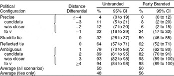
Table 1 shows the percentage of people who chose the ambiguous candidate in each of the four key political configurations: precise candidate closer (Type I), ambiguous candidate closer (Type II), straddle tie (Type III), and reflected tie (Type IV). Footnote ¹¹ The distance differential measures the voter's absolute distance to the precise candidate, minus the voter's absolute distance to the midpoint of the ambiguous candidate's interval (i.e., |v − p| − |v − μ|). The distance differential ranged from –5 to 5; we grouped –4 with –5 and 4 with 5 to increase the sample sizes at the extremes.

TABLE 1.

Rates at Which Respondents Chose the Ambiguous Candidate

Note: For each scenario, the table gives the percentage of respondents who favored the ambiguous candidate over the precise one. The distance differential is the absolute distance from the respondent to the precise candidate's policy position, minus the absolute distance from the respondent to the midpoint of the vague candidate's policy interval. Total sample size was 1,299 in the unbranded condition and 1,241 in the party branded condition. The averages at the bottom of the table are unweighted means.

Table 1 reveals two clear patterns. First, proximity strongly influences the decisions of voters (see also Tomz and Van Houweling Reference Tomz and Van Houweling2008). According to proximity theory, ambiguous candidates are at an electoral disadvantage when the distance differential is negative, but they enjoy an electoral advantage when the differential is positive. Our data are highly consistent with this expectation. In the unbranded condition, support for the ambiguous candidate increased from a low of 4% when the difference differential was −4 or less, to a high of 94% when the ambiguous candidate enjoyed a proximity advantage of at least 4 points. Data from the party branded condition display an even stronger pattern. As the difference differential shifted from its minimum to its maximum value, the ambiguous candidate went from having no supporters to enjoying almost unanimous backing.Footnote ¹²

Second, and just as striking, ambiguity appears to carry no significant cost. Averaged across all scenarios in Table 1, with or without party brand names, respondents were as likely to choose the ambiguous candidate as they were to choose the precise one. Ambiguity proved innocuous even when restricting attention to ties, situations in which the voter was equidistant to the precise candidate and the midpoint of the vague candidate's interval. In the unbranded condition, 48% of voters who faced ties liked the ambiguous candidate more than the precise one. In the party branded condition, 56% of ties went to the ambiguous candidate, suggesting that ambiguity benefitted candidates in partisan elections. We return to this theme later in the article.

The reflected ties in Table 1 are of special interest. In polarized political environments, candidates of different parties generally take distinct positions, making reflected ties far more common than straddle ties. Centrist or “swing” voters—the ones most likely to determine elections—are especially likely to encounter reflected ties because partisan candidates often distribute themselves on opposite sides of the political center. When reflected ties arose in our sample, a substantial majority of voters (64% in the unbranded condition and 62% in the party branded condition) preferred the ambiguous candidate.Footnote ¹³

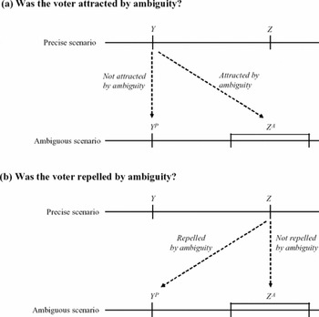
To check the robustness of these findings, we next conducted a within-subject analysis. In particular, we compared how each voter responded to a pair of precise candidates versus how the same voter responded to an otherwise identical scenario in which one of the candidates took an ambiguous position. For the purpose of illustration (Figure 2), consider a “precise” scenario in which candidates Y and Z locate at specific points, and an “ambiguous” scenario in which candidate Y^P locates precisely at Y, but candidate Z^A announces an ambiguous platform centered on Z. In this setting, Y^P is a replica of Y and Z^A is an ambiguous analog to Z.

FIGURE 2.

Within-Subject Tests of the Effects of Ambiguity

The choices that voters make in scenarios like these can reveal whether they are attracted to or repelled by ambiguity. As Figure 2a illustrates, voters who chose Y in the precise scenario could have been attracted by ambiguity. Those who opted for Z^A in the ambiguous scenario were in fact attracted by ambiguity, whereas those who selected Y^P were not attracted by ambiguity. Figure 2b displays the other logical possibilities. Voters who chose Z in the precise scenario could have been repelled by ambiguity. Among them, voters who defected to Y^P in the ambiguous scenario were repelled by ambiguity, whereas voters who chose Z^A were not.

We presented people with matched pairs like the one in Figure 2. In half the cases, we denoted each of the four candidates with a unique letter. In the other half, we referred to the leftmost candidate as a Democrat and the rightmost candidate as a Republican. For each matched pair, we recorded the respondent's choice pattern: attracted to ambiguity (Y, Z^A), not attracted to ambiguity (Y, Y^P), repelled by ambiguity (Z, Y^P), or not repelled by ambiguity (Z, Z^A).

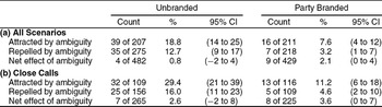
Table 2 reports the rates at which voters were attracted to or repelled by ambiguity, and it summarizes the net effect. When we analyzed all available cases (Table 2a), nearly 19% of the 207 respondents who could have been attracted by ambiguity actually chose the ambiguous candidate. In contrast, less than 13% of the 275 respondents who might have been repelled by ambiguity were in fact turned away. Rates of attraction and repulsion were lower (about 8% and 3%, respectively) in the party branded condition, where most respondents consistently chose the candidate from their own party in both the precise and the ambiguous scenarios.

TABLE 2.

Within-Subject Estimates of the Effects of Ambiguity

Note: There were 482 matched pairs involving unbranded candidates and 429 involving party branded candidates. Panel (a) includes all available cases. Panel (b) includes only “close calls” in which the distance differential was either 0 or 1.

On balance, ambiguity had neutral or slightly positive effect on the fortunes of political candidates. By making vague rather than precise policy statements, an unbranded candidate could gain 0.8% of the total vote, and a branded candidate could win the support of an additional 2.1% of the electorate.

The apparent rewards for ambiguity were larger for close calls: scenarios with a distance differential of 0 or 1 (Table 2b). These cases were especially informative because the distance differential was less likely to override the consequences of ambiguity. In close calls, ambiguity improved the vote share of unbranded candidates by 2.6 percentage points and the vote share of partisan candidates by 3.6 percentage points. Thus, the within-subject tests reinforce the conclusions from the between-subject tests: ambiguity is not costly and may, in fact, help candidates win close elections.

Why do so many voters in our study seem to support candidates with ambiguous messages? How do the individual characteristics of voters affect whether they are attracted to or repelled by ambiguity? Why do voters respond somewhat differently in the branded and unbranded conditions? The next four sections explore these questions in greater detail, using four distinct analytical techniques.

Using Ties to Test Causal Mechanisms

As a first step toward isolating causal mechanisms, we exploited the special characteristics of ties. Triple conjunctions (scenarios in which v = p = μ) are especially interesting because the voter cannot gain and may, in fact, lose by selecting the risky candidate. Thus, in a triple conjunction, neither risk acceptance nor optimism can explain why the voter would choose the ambiguous candidate. When our respondents faced triple conjunctions, though, they selected the ambiguous option 25% of the time when candidates were unbranded and 40% of the time when candidates were party branded.

What explains this pattern? One possibility, suggested previously, is that voters value flexibility and think ambiguous candidates are more willing to adapt to changing circumstances. A second possibility, which applies only to the party branded condition, is blind party bias. Perhaps citizens break ties not by determining which candidate presents less risk, but by blindly selecting the candidate from their own party. If such bias were ubiquitous, respondents in our experiment, which randomized party labels, would have chosen the vague candidate around 50% of the time. By comparing reactions to triple conjunctions in the branded versus unbranded conditions, however, one sees that pure party bias could have boosted the fortunes of ambiguous candidates by only about 40 − 25 = 15 percentage points. A final possibility is pure error. Perhaps respondents made mistakes, either by not paying attention to the question or by accidentally choosing the candidate they did not intend to pick. Other research on issue voting, though, found a baseline error rate of only 15.5% (Tomz and Van Houweling Reference Tomz and Van Houweling2008, 312), far short of the rate at which our respondents chose the ambiguous candidate.

To estimate how much behavior could be due to risk acceptance and/or optimism, we compared triple conjunctions with double conjunctions (scenarios in which p = μ ≠ v). When candidates were unbranded, respondents opted for the vague candidate 34% of the time when facing double conjunctions versus 25% of the time when facing triple conjunctions. Some combination of risk acceptance and optimism could, therefore, be responsible for around 26% ((34−25)/34 = 0.26) of the preference for vague candidates. In the party branded scenarios, support for the ambiguous candidate was 52% with double conjunctions versus 40% with triple conjunctions. Thus, about 23% ((52−40)/52 = 0.23) of votes for party branded vague candidates could be due to risk acceptance or optimism. In summary, existing theories can explain only part of voters' preferences for ambiguity.

Using Probit Regression to Test Causal Mechanisms

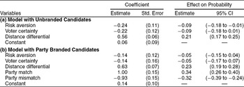
We next used probit regression to test causal mechanisms. Our dependent variable took a value of 1 if the respondent chose the ambiguous candidate and a value of 0 otherwise. The model with unbranded candidates included three explanatory variables. The first, risk aversion, tested whether respondents' attitudes toward risk affected their willingness to gamble on imprecise candidates. Our measure of risk aversion was 1 if respondents said they preferred to avoid taking risks and 0 otherwise.Footnote ¹⁴ The second independent variable measured voters' certainty about their own location. We reasoned that respondents who were certain of their own position would dislike vague candidates, whereas other respondents would exhibit the opposite tendency. Our measure singled out people who expressed extreme certainty about their location on the government services and spending scale. Finally, we controlled for the distance differential, which proved important in Table 1 and is central to proximity theory. The distance differential, which ranged from –5 to 5 with a modal value of 0, should have a positive effect on the probability of selecting the ambiguous candidate.

Table 3a presents the estimates from our probit regression with unbranded candidates.Footnote ¹⁵ The first numeric columns give coefficients and standard errors, and the remaining columns show how a one-unit increase in the explanatory variable affected the probability of choosing the ambiguous candidate. Other factors equal, risk-averse citizens were about 9 percentage points less likely to choose the ambiguous candidate. This effect was substantively large, and its 95% confidence interval was strictly negative. Similarly, citizens who were certain about their own position were 9 percentage points less likely to embrace ambiguity, although the confidence interval slightly overlapped zero. Finally, the large positive coefficient on distance differential fit the central prediction of proximity theory: voters prefer the candidate closest to themselves.

TABLE 3.

Probit Regression Analyses of Preference for the Ambiguous Candidate

Note: Coefficients and robust standard errors come from probit regressions in which the dependent took a value of 1 if the respondent chose the ambiguous candidate and a value of 0 otherwise. “Effect on Probability” shows how a one-unit increase in the explanatory variable would change the probability of choosing the ambiguous candidate, starting from a baseline in which the respondent was indifferent between the ambiguous and the precise candidates. Sample sizes are 647 in the model with unbranded candidates and 627 in the model with party branded candidates.

Our model with party branded candidates included the same three explanatory variables plus measures of party affiliation, which could affect votes in two ways. First, partisanship could distort perceptions about the locations of candidates. Respondents might be optimistic about the positions of vague candidates from their own party (partisan optimism) and/or pessimistic about the positions of vague candidates from the opposite party (partisan pessimism). Second, partisanship could trigger blind bias: voters might favor candidates from their own party and disfavor members of the opposition, regardless of the candidates' vague or precise policy statements.

In our model with branded candidates, party match was 1 if the voter and the ambiguous candidate belonged to the same party; party mismatch was 1 if they belonged to different parties. Independent voters, who neither matched nor mismatched the party of the ambiguous candidate, were the reference category.

As Table 3b shows, the introduction of party brand names muted the effects of risk aversion and voter certainty. When candidates were identified as Democrat or Republican, risk aversion and respondent certainty each lowered the preference for the ambiguous candidate by about 5 percentage points, an amount statistically indistinguishable from zero at standard confidence levels. Distance differential, however, continued to have strong effects even in the presence of party brands. Finally, party affiliation influenced choices. The probability of selecting the vague candidate was 34 percentage points higher when the respondent and the candidate belonged to the same party, but was 32 percentage points lower when they belonged to different parties.

Using Imputed Locations to Test Causal Mechanisms

From the cross-sectional probit, we could not tell whether the effects of partisanship arose entirely from blind partisan bias, or whether partisan optimism and pessimism were also at work. To shed light on this important question, we analyzed another type of data. Our experiment asked voters not only to choose between vague and precise candidates, but also to indicate where they expected ambiguous candidates to stand. For each voter, define imputation bias as B = |v − μ| − |v − μ_I|, where v is the voter's bliss point, μ is the midpoint of the ambiguous candidate's policy interval (which we regard as an unbiased reading of the candidate's position), and μ_I is the location the voter imputed to the ambiguous candidate. Positive values of B imply optimism, in which respondents shifted the vague candidate's probability distribution toward their own ideal point. Negative values of B, in contrast, reveal pessimism, in which respondents skewed the candidate's probability distribution away from themselves. B = 0 means no bias in either direction.

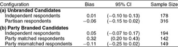
Table 4 presents the average value of B, conditional on the party affiliations of the voter and the candidate. Table 4 supports three inferences. First, there is little evidence of general optimism. Independent voters believed that unbranded candidates were only 0.01 scale points closer and that branded candidates were only 0.05 scale points closer than an unbiased estimate would suggest. These levels of optimism were statistically indistinguishable from zero. Partisan voters were slightly pessimistic about unbranded candidates, but not at statistically significant levels. Overall, then, respondents offered fairly objective assessments when party was not a factor.

TABLE 4.

Average Bias in Imputed Distance to Candidates

Note: Bias is measured as expected distance (the distance from the voter to the midpoint of the ambiguous candidate's policy interval) minus imputed distance (the distance from the voter to where the voter believed that the ambiguous candidate stood).

Second, we find strong evidence of partisan optimism. Democrats and Republicans perceived ambiguous candidates from their own party as 0.32 scale steps closer to themselves than to the midpoint of the vague interval. The 95% confidence interval ranged from 0.20 to 0.43 points, affording great certainty that people viewed members of their own party through rose-colored glasses. Third, we found much less evidence of partisan pessimism. Voters moved candidates from the opposite party only 0.11 points further from their self-locations than an objective analysis of candidate positions would dictate. This effect was statistically insignificant at conventional levels. Thus, our analysis uncovered an asymmetry, in which partisan optimism exceeded partisan pessimism in both magnitude and statistical significance.

Using Within-Subject Data to Test Causal Mechanisms

If the optimism–pessimism asymmetry influences behavior, then ambiguity should help candidates gain votes from members of their own party without losing much support from members of other parties. We tested this hypothesis by applying within-subject methods (as in Figure 2 and Table 2) to three mutually exclusive and exhaustive subgroups of our party branded sample.

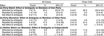
Respondents in the first subgroup considered a scenario with two precise candidates, and also considered an equivalent scenario in which their own party's candidate was ambiguous (Table 5a). In the scenario involving two precise candidates, 14 of 114 people voted for the opposition.Footnote ¹⁶ Seven of them instead chose their own party's candidate when that candidate was ambiguous. Thus, ambiguity enabled candidates to attract half of the attractable respondents from their own party. In contrast, ambiguity drove away only 1 of the 100 people who potentially could have been repelled. On balance, ambiguous candidates outperformed precise candidates by 5.3 percentage points among members of their own party. Ambiguity proved even more beneficial in close calls (when the candidates were exactly or nearly equidistant from the voter). In those cases, ambiguity swelled support among copartisans by more than 10 percentage points.

TABLE 5.

Within-Subject Estimates, by Party Match

Note: Panels (a)–(c) are a mutually exclusive and exhaustive partition of the 429 matched pairs from the party branded sample in Table 2. Close calls are cases in which the distance differential was either 0 or 1.

Respondents in the second subgroup encountered an ambiguous candidate from the other party, instead of their own party (Table 5b). In these party mismatched cases, ambiguity drew 4 of the 113 respondents who could have been attracted, while driving away 4 of the 23 respondents who could have been repelled. Thus, ambiguity attracted exactly as many voters as it repelled. The same pattern held in close-call scenarios. Overall, then, ambiguity neither increased nor decreased support by members of the opposite party.

The final subgroup of our party branded sample contained independents (Table 5c). Among this group, the net effect of ambiguity was slightly positive. Ambiguity raised support among independents by 1.7 percentage points in the sample as a whole and by 3.1 percentage points in close-call scenarios. The confidence intervals around both effects overlapped zero, however.

These findings, combined with previous ones, paint a consistent picture about the effects of ambiguity in partisan elections. Citizens are optimistic about where ambiguous candidates from their own party stand. Setting aside other potential consequences of ambiguity, this selective optimism makes ambiguity an advantageous strategy for candidates who want to increase their vote share among members of their own party. At the same time, people fairly perceive the positions of ambiguous candidates from the opposite party, instead of assuming the worst about them. Other factors equal, then, ambiguity does not undermine candidates' attempts to woo voters from the other party. Thus, in partisan elections, ambiguity may help candidates more than it hurts them.

The Range of Ambiguity

In August–September 2008, we conducted a nationally representative survey that measured how much ambiguity people perceived in statements by John McCain (R) and Barack Obama (D) on the issue of government services and spending.Footnote ¹⁷ People placed the candidates on the same seven-point issue scale used in our experiments. Departing from the standard practice in surveys, we allowed respondents to express the ambiguity in candidate statements by selecting multiple points on the scale.Footnote ¹⁸

To familiarize respondents with our format and encourage them to use multiple points when appropriate, we displayed four examples of candidates. The first candidate said the government should increase services by a small amount. We showed respondents how to place this candidate at the corresponding point on the scale. The second candidate said the government should increase services, but was vague about the amount. We demonstrated how to place this candidate, by choosing all three points in the implied range from increase by a small amount to increase by a large amount. The third candidate said that the government should not increase services, but was vague about which of the remaining options he or she favored. We taught respondents to summarize such statements by selecting four points, ranging from keep services the same to decrease services by a large amount. The final candidate was totally vague when saying whether the government should increase services, decrease services, or keep them the same. We instructed respondents to place a candidate like this across all seven points.

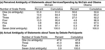
After providing these examples, we asked respondents to summarize what McCain and Obama had said about the issue (Table 6a).Footnote ¹⁹ Overall, 51% of people who evaluated McCain's statements put them at a single point, and an additional 34% saw the statements as straddling two or three scale points. Similarly, 51% perceived Obama's statements as occupying one point, and 42% felt the statements encompassed two or three points.

Table 6a supports two conclusions. First, many people believed that the presidential candidates were making ambiguous policy statements about government services such as health and education. Second, the vast majority—around 90%—perceived a range of ambiguity like the one in our experiments.

TABLE 6.

Perceived and Actual Ambiguity of Candidate Statements on Fiscal Issues

Note: Panel (a) is based on a public opinion survey in which 478 people offered evaluations of McCain's statements and 589 offered evaluations of Obama's statements. Panel (b) is based on analysis of all 429 prospective statements about tax policy that candidates from either party made in presidential primary and general election debates (2007–2008), and in the vice presidential debate (2008).

For additional evidence about candidate ambiguity in actual campaigns, we catalogued statements by presidential and vice presidential candidates in 2007–2008 on a related fiscal issue, federal tax policy. Our analysis covered all tax policy proposals by all participants in 25 Democratic and 15 Republican primary debates and in 4 general election debates. There were 489 proposals; 88% pertained to the level of taxation and thus could be put on a scale like the one we used in our experiment. The remaining 12% called for systemic reform such as replacing the income tax with a national consumption tax. We discuss the statements about tax levels now and revisit the systemic statements later in the article.

We coded each statement based on two criteria. First, did the candidate advocate increasing taxes, decreasing taxes, keeping taxes the same, or some combination of the three? Second, did the candidate specify the magnitude of any proposed change? We regarded candidates as specific if they offered a precise proposal (e.g., “change the marginal rate from 33% to 39%” or “eliminate the capital gains tax”).

Based on these criteria, we coded the maximum number of scale points each proposal spanned. As Table 6b shows, 48% of statements called for a specific change or unequivocally advocated keeping taxes the same, implying no ambiguity. An additional 41% of statements spanned three points because the candidate advocated increasing or decreasing taxes but did not say how much. Around 10% of statements covered four points because the candidate held open two options: either keeping taxes the same or changing them in a particular direction. Finally, only 1% of statements were totally vague because they did not make clear whether the candidate would raise, sustain, or lower the particular tax being discussed. This analysis reinforces the lessons from our survey: candidates speak vaguely about fiscal issues, but they typically limit their ambiguity to the levels in our experiments.

Types of Ambiguity

Of course, ambiguity comes in other forms, including broad but vacuous statements about policy goals. During the 1952 presidential campaign, for example, Dwight Eisenhower pledged “I shall go to Korea” with the purpose of ending the war. Richard Nixon was similarly vocal about goals but silent about means: in the 1968 campaign, he promised “new leadership” to end the Vietnam war.

We found equally ambiguous goal-focused statements about taxes in the 2007–2008 presidential debates. Recall that around 12% of statements advocated systemic tax reform. Of these, 17% (comprising 2% of the entire sample) announced sweeping goals (e.g., “changing the entire tax system” to make it “fairer,” “less oppressive,” and less beholden to “special interests”) without mentioning particular tax instruments. These kinds of ambiguous statements, although rare, may have different consequences than ones in our experiments.

Another form of candidate ambiguity arises when candidates espouse inconsistent positions. Senator John Kerry famously voted to authorize the use of U.S. force in Iraq in 2002, only to renounce the war when running for president two years later. In the 2008 presidential campaign, John McCain proposed to extend tax cuts that he had vigorously opposed years earlier. Experiments and historical analyses could help quantify the costs and benefits of intertemporal inconsistency, or “flip-flopping.”

Some candidates take inconsistent stands even within a single speech. In a 2007 Democratic primary debate, for example, Congressman Dennis Kucinich said he would not increase taxes. However, in the next breath, he pledged to repeal the tax cuts that President Bush had given to the richest Americans. These kinds of logical inconsistencies appeared in only 2 of the 489 tax proposals we examined, but may be more common in other issue areas.

Finally, ambiguity arises when candidates send implicit, rather than explicit, messages. In the late 1960s, gubernatorial candidate George Wallace “gained legitimacy for himself through ambiguity” (Mendelberg Reference Mendelberg2001, 91; see also Chester, Hodgson, and Page Reference Chester, Hodgson and Page1969). Wallace used symbols to attract racist voters without employing segregationist language that other people would have found offensive. Researchers could design experiments like the one in Mendelberg (Reference Mendelberg2001, 191–208) to compare the effects of implicit versus explicit messages on a wide range of campaign issues.

More generally, the effects of ambiguity could vary by issue. We focused on government services and spending, the central dimension that parties have contested since the New Deal. Ambiguity may evoke different responses on other issues, such as complex debates about health care reform and global warming, or moral debates about abortion and gay marriage.

Although our experiments examined a ubiquitous type of ambiguity in doses that candidates commonly use, one must be careful about extrapolating our conclusions to other types and levels of ambiguity. Voters may, for example, accept ambiguity within the range we studied but shun candidates who are totally vague. This hypothesis, if correct, could explain why candidates in the 2008 presidential campaign delivered vague messages but stopped short of total ambiguity. Our experimental template—unlike observational studies—could be used to infer the consequences of levels and types of ambiguity that politicians rarely employ.