1 Introduction
The upslope, shoreward transport of colder, nutrient-rich waters from below the ocean thermocline is thought to be critical to the functioning of coastal ecosystems such as coral reefs and kelp forests (Leichter et al. Reference Leichter, Wing, Miller and Denny1996). Internal bores generated by the breaking of shoaling internal waves on the slope provide a mechanism for this cross-shelf transport of dense water (Wallace & Wilkinson Reference Wallace and Wilkinson1988). As internal waves propagate into shallow water, the waves steepen, which can lead to breaking and, at times, the generation of turbulent bores of dense fluid (e.g. Helfrich Reference Helfrich1992; Aghsaee, Boegman & Lamb Reference Aghsaee, Boegman and Lamb2010). These formations of subthermocline water continue to travel inshore, mixing with ambient surface water (Wallace & Wilkinson Reference Wallace and Wilkinson1988; Holloway Reference Holloway and Parker1991; Pineda Reference Pineda1994).
The propagation of internal bores is a significant mechanism for the transfer of nutrients, sediment and larvae between deep waters and the shelf environment (Ivey, Winters & DeSilva Reference Ivey, Winters and DeSilva2000; Sharples, Moore & Abraham Reference Sharples, Moore and Abraham2001; Hosegood, Bonnin & van Haren Reference Hosegood, Bonnin and van Haren2004; Scotti & Pineda Reference Scotti and Pineda2004; Bourgault, Kelley & Galbraith Reference Bourgault, Kelley and Galbraith2008). In addition, bores may provide localized, intermittent cooling relief from the warmer, ambient surface waters around coral reefs, which may help to explain the patchy distribution of coral bleaching (Leichter et al. Reference Leichter, Wing, Miller and Denny1996; Goreau et al. Reference Goreau, McClanahan, Hayes and Strong2000; Reigl & Piller Reference Reigl and Piller2003; West & Salm Reference West and Salm2003). Despite numerous observations of internal bores in coastal regions all over the world (Colosi et al. Reference Colosi, Beardsley, Lynch, Gawarkiewicz, Chiu and Scotti2001; Morozov et al. Reference Morozov, Trulsen, Velarde and Vlasenko2002; Klymak & Moum Reference Klymak and Moum2003; Scotti & Pineda Reference Scotti and Pineda2004; Leichter, Deane & Stokes Reference Leichter, Deane and Stokes2005; Pritchard & Weller Reference Pritchard and Weller2005; Bourgault et al. Reference Bourgault, Blokhina, Mirshak and Kelley2007; Walter et al. Reference Walter, Woodson, Arthur, Fringer and Monismith2012), several questions remain regarding internal bore generation and propagation.
Even with the progress being made in the field to obtain higher resolution temporal and spatial data of internal bores (Walter et al. Reference Walter, Squibb, Woodson, Koseff and Monismith2014), laboratory experiments and numerical simulations have been extensively used to study shoaling internal waves. Previous studies have focused on several aspects of these phenomena, including breaking and run-up mechanisms (Cacchione & Wunsch Reference Cacchione and Wunsch1974; Kao, Pan & Renouard Reference Kao, Pan and Renouard1985; Saffarinia & Kao Reference Saffarinia and Kao1996; Michallet & Ivey Reference Michallet and Ivey1999; Lamb Reference Lamb2001; Vlasenko & Hutter Reference Vlasenko and Hutter2002; Lamb Reference Lamb2003; Umeyama & Shintani Reference Umeyama and Shintani2006; Lim, Ivey & Nokes Reference Lim, Ivey and Nokes2008; Umeyama Reference Umeyama2008), energetics and reflection (Nagashima Reference Nagashima1971; Thorpe Reference Thorpe1987; Boegman, Ivey & Imberger Reference Boegman, Ivey and Imberger2005; Nakayama & Imberger Reference Nakayama and Imberger2010), bottom boundary layer characteristics (Taylor Reference Taylor1993; Ivey et al. Reference Ivey, Winters and DeSilva2000; Boegman & Ivey Reference Boegman and Ivey2009) and characteristics of turbulence and mixing (Ivey & Nokes Reference Ivey and Nokes1989; Helfrich Reference Helfrich1992; De Silva, Imberger & Ivey Reference De Silva, Imberger and Ivey1997). In comparison, few experiments have investigated the conditions under which shoaling internal waves generate internal bores, as well as the characteristics of the bores themselves.
Of those studies encompassing the topic of internal bores, often referred to as boluses in laboratory settings, two distinct categories of trial can be identified: those incorporating either an idealized continental slope-shelf topography, or those using a uniform slope. For cases with an idealized shelf, bolus formation on the shelf was found to be related to forcing and the vertical excursion of the densest fluid. For example, in a laboratory scale numerical simulation of first-mode internal waves in a linearly stratified fluid, Venayagamoorthy & Fringer (Reference Venayagamoorthy and Fringer2007) related bolus formation to the dimensionless steepness of the incoming wave
 $Fr=U_{0}/C_{ph}$
and a dimensionless slope parameter
 ${\it\gamma}/s$
. Here,
 $U_{0}$
is the maximum velocity amplitude,
 $C_{ph}$
is the linear first-mode internal wave speed in a linearly stratified fluid,
 ${\it\gamma}$
is the topographic slope and
 $s$
is the slope of the internal wave beam. Using the methodology suggested by Venayagamoorthy & Fringer (Reference Venayagamoorthy and Fringer2007), bolus formation was quantified by calculating the vertical displacement of the densest fluid on the shelf in relation to its equilibrium position off the shelf. Here, greater vertical displacements of fluid on the shelf indicate stronger bolus formation. Results indicate that formation of boluses across the shelf break is highly dependent on
 $Fr$
, where for increasing values of
 $Fr$
, greater vertical displacements of fluid are observed. A lower bound for the formation of boluses was successfully calculated, but an upper limit above which boluses no longer form was not observed in this study.
More recently, using direct numerical simulations (DNS), Arthur & Fringer (Reference Arthur and Fringer2014) investigated the structure and energetics of breaking internal waves on slopes for a laboratory scale flow very similar to our study. Seven cases with varying initial wave amplitude and bathymetric slope, but constant wave Reynolds number
 $Re_{w}$
, were considered. They found that the majority of dissipation (63 %) occurs along the no-slip bottom boundary, and that most of the remaining dissipation (35 %) and nearly all irreversible mixing occurs in the interior after breaking, when density overturns are present at the interface. Breaking introduces three-dimensionality to the flow field that is driven by the lateral breakdown of density overturns and the lobe–cleft instability typical of gravity currents. The resulting longitudinal rolls (streamwise vorticity) increase dissipation by roughly 8 % and decrease irreversible mixing by roughly 20 % when compared with a similar two-dimensional simulation. Finally they found that the bulk mixing efficiency is shown to increase for larger and smaller values of the internal Iribarren number
 ${\it\xi}$
, with a minimum for intermediate values of
 ${\it\xi}$
and a peak near
 ${\it\xi}=0.8$
for plunging breakers.
Large vertical displacements of dense fluid on the shelf were also observed by Lim, Ivey & Jones (Reference Lim, Ivey and Jones2010) in a set of laboratory experiments designed to analyse internal wave generation by barotropic tidal forcing in a linearly stratified fluid. Defining a non-dimensional vertical excursion parameter
 ${\rm\Delta}hN/W_{0}$
, where
 ${\rm\Delta}h$
is the vertical excursion of the fluid particles from their initial position,
 $N$
is the buoyancy frequency and
 $W_{0}$
is the near-bottom vertical velocity associated with the local depth-averaged velocity, Lim et al. (Reference Lim, Ivey and Jones2010) found that bolus features were observed for cases when
 ${\rm\Delta}hN/W_{0}>3.2$
. To classify bolus generation, Lim et al. also employed a generation parameter
 $G=Re/({\it\gamma}/s)$
in which
 $G$
compares the wave inertia to the stabilizing effects of buoyancy and viscosity. In this case,
 $Re=U_{0}^{2}/N{\it\nu}$
, where
 $U_{0}$
is the amplitude of the deep-water barotropic tidal velocity and
 ${\it\nu}$
is the fluid viscosity. The resulting flow regime boundaries were reported: for
 $G<3$
only a wave beam was observed, for
 $3<G<50$
both a beam and a bolus were observed, for
 $50<G<400$
only boluses were observed and for
 $G>400$
no boluses were observed, indicating a regime in which bolus formation is suppressed. However, the formation mechanism that controls the suppression of bolus formation in highly nonlinear cases was not explored.
Studies observing boluses on uniform slopes have addressed several concepts of shoaling internal waves. In some of the earliest conducted laboratory experiments, Wallace & Wilkinson (Reference Wallace and Wilkinson1988) showed that as two-layer periodic wave trains steepened on a shallow slope, they became kinematically unstable and eventually overturned, creating a bolus of dense fluid which propagated further upslope. From their observations, the authors established that once a bolus stabilizes after wave breaking, it becomes self-preserving in nature. The parameters of the bolus, such as celerity and density, can then be expressed by simple power laws involving a normalized run-up distance and coefficients depending on surface area, added mass and drag. However, Wallace & Wilkinson (Reference Wallace and Wilkinson1988) note that they found no dependence of wave breaking on the wave forcing conditions, which could be a result of the incorporation of only shallow slopes (0.030 and 0.054) and relatively low wave forcing.
Helfrich (Reference Helfrich1992) found similar results for bolus celerity in laboratory trials examining the approach of solitary waves of depression on a slope. However, whereas Wallace & Wilkinson (Reference Wallace and Wilkinson1988) observed only one bolus, Helfrich (Reference Helfrich1992) noted the formation of multiple boluses for a single wave breaking event due to the scattering nature of the wave of depression on the slope. The number and size of the boluses generated by each wave were also examined. Like Wallace & Wilkinson (Reference Wallace and Wilkinson1988), the range of wave amplitudes and slopes (0.034, 0.050 and 0.067) were limited to comparatively low values.
Aghsaee et al. (Reference Aghsaee, Boegman and Lamb2010) extended the range of topographic slopes and wave forcing studied in two-dimensional numerical simulations of solitary waves of depression on slopes. Following the concepts introduced by Boegman et al. (Reference Boegman, Ivey and Imberger2005), the character of wave breaking was classified into three distinct regimes: surging, plunging or collapsing. Analysis of their simulations revealed a complicated relationship between the separation of the breaking types and the wave slope. Here the wave slope was defined as
 $S_{w}=a/L_{w}$
, where
 $L_{w}$
is a measure of half of the wavelength and
 $a$
is the wave amplitude. The authors noted that after all wave breaking processes, cores of mixed fluid, which they termed boluses, form close to the wave surging region and are pushed inshore. The number and size of boluses generated were found to be similar to those reported by Helfrich (Reference Helfrich1992), however the characteristics of the boluses in relation to the type of wave breaking were not discussed.
We add to the work described above by examining the formation and propagation of internal boluses from breaking internal wave trains on a uniform slope in a two-layer stratified fluid. In this study, a bolus is defined as a vortex of dense fluid created by a shoaling internal wave that is then pushed further up the slope by the dynamics of the breaking wave. Bolus formation from periodic wave trains is qualitatively explored and compared with observations made by studies employing different wave types. Additionally, the physical conditions for both bolus formation and limitation are explored, as well as how the characteristics of the boluses relate to these conditions. In an effort to link the results with oceanic observations, these physical conditions are expressed with quantities that are more readily measured in the field. Using topographic and incident wave properties, we have developed simple dynamic parameters to describe the initial flow conditions, including a wave Reynolds number, a Froude number and a wave steepness parameter. We then use these parameters to address the following overarching questions:
-
(i) What flow mechanisms govern the formation of internal boluses?
-
(ii) How does bolus formation depend on the incident wave conditions, such as wave amplitude and frequency?
-
(iii) How do the physical characteristics of the resulting boluses depend on the initial flow conditions?
These questions are explored through a series of laboratory experiments using a high-resolution imaging system to employ planar laser-induced fluorescence (PLIF) and particle image velocimetry (PIV).
The layout of this paper is as follows. In § 2, the laboratory facility and experimental methods are described. The results and their physical interpretation are presented in § 3, with overall conclusions given in § 4.
2 Experimental methods
2.1 Facility
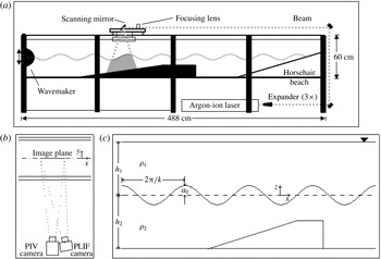
Laboratory experiments were conducted in the Stanford University Environmental Fluid Mechanics Laboratory internal wave facility, shown in figure 1. The facility (figure 1
a; see Troy & Koseff Reference Troy and Koseff2005a
) consists of an enclosed rectangular tank 30 cm wide, 60 cm tall and 488 cm long with a semi-cylindrical, vertically oscillating wavemaker mounted at one end to generate interfacial waves. Trains of progressive, interfacial waves were forced over a uniform sloped shelf of approximately
 $12^{\circ }$
with a final height of 30 cm.
(a) Schematic of tank with laser and set-up for PLIF/PIV imaging system. (b) Aerial view of camera set-up for simultaneous PLIF/PIV. (c) Key wave parameters.

A two-layer stratification was achieved using two salt solutions with an overall density difference
 ${\rm\Delta}{\it\rho}/{\it\rho}_{0}=2({\it\rho}_{2}-{\it\rho}_{1})/({\it\rho}_{2}+{\it\rho}_{1})=1\,\%$
between the two layers. Here,
 ${\rm\Delta}{\it\rho}={\it\rho}_{2}-{\it\rho}_{1}$
is the density difference between the lower and upper layer densities respectively, and
 ${\it\rho}_{0}=({\it\rho}_{2}+{\it\rho}_{1})/2$
is the average density. In order to prevent the distortion of the interface due to light refraction for the quantitative imaging experiments, a dilute isopropyl alcohol solution was used in place of salt in the upper layer in order to match the index of refraction between the stratified layers. A conductivity–temperature probe mounted on a vertical traverse was used to obtain density profiles to verify the initial stratification. To maintain a thin density interface between trials, fluid was withdrawn from the interfacial region using a thin slotted pipette attached to a pump and positioned at the density interface. Before each experiment, the interface was sharpened so that 99 % of the density variation occurred over the interfacial thickness
 ${\it\delta}=1.1~\text{cm}\pm 0.2~\text{cm}$
. During the experiments, the upper and lower water depths
 $h_{1}$
and
 $h_{2}$
were kept constant at 30 cm and 26 cm, respectively.
Interfacial waves of varying incident amplitude
 $a_{0}$
and wavelength
 ${\it\lambda}=2{\rm\pi}/k$
were generated by varying the wavemaker stroke and frequency
 ${\it\omega}$
, where
 $k$
is defined as the wavenumber (see figure 1
c). The incident amplitude
 $a_{0}$
was determined by measuring the variation in the interface height at a point upstream of the slope before the waves began to feel the effect of the bottom topography. The wavemaker forcing frequency
 ${\it\omega}$
determines the wavenumber
 $k$
in a given stratification, according to the two-layer thin-interface dispersion relation:
 $$\begin{eqnarray}\displaystyle {\it\omega}^{2}=gk\frac{2({\it\rho}_{2}-{\it\rho}_{1})}{({\it\rho}_{2}+{\it\rho}_{1})}\frac{1}{\coth (kh_{1})+\coth (kh_{2})}. & & \displaystyle\end{eqnarray}$$
The wave amplitude was varied so that the incident amplitude measured from the beginning of the slope was
 $a_{0}=0.80{-}5.6~\text{cm}$
and the wave frequency was varied from
 ${\it\omega}=0.25{-}1.17~\text{rad}~\text{s}^{-1}$
, corresponding to a wavelength range of
 ${\it\lambda}=27{-}255~\text{cm}$
. Additional details of the facility and imaging set-up are described in Troy & Koseff (Reference Troy and Koseff2005a
,Reference Troy and Koseff
b
).
2.2 Flow visualization techniques
Both PLIF and PIV were used to obtain qualitative and quantitative measurements of the flow field in two dimensions. The imaging set-up is presented in figure 1(a,b).
To achieve high-resolution images of the density field using PLIF, the lower layer was dyed with a laser fluorescent dye (Rhodamine 6G) at a concentration of 50–80 ppb. Since Rhodamine dye and salt have similar Schmidt numbers (
 $Sc={\it\nu}/{\it\kappa}$
, 600–1200 and 700 respectively, where
 ${\it\kappa}$
is the molecular diffusivity and
 ${\it\nu}$
is the viscosity), and hence similar diffusivities, the laser-induced fluorescence of the dye is directly related to the salinity of the fluid (Rehmann Reference Rehmann1995). Image pixel intensity can thus be converted to dye concentration and subsequently to density after appropriate calibration (Crimaldi & Koseff Reference Crimaldi and Koseff2001; Troy & Koseff Reference Troy and Koseff2005a
). A computer controlled scanning mirror was used to generate a light sheet of approximately 0.5 mm thickness at its thinnest point from an argon ion laser beam, illuminating the dye in a two-dimensional plane. Images were acquired using a
 $1024\times 1024$
pixel, 12-bit grey scale CCD camera (Silicon Mountain Designs). Spatial resolution ranged from 0.1 to 0.5 mm, depending on the image focus of the experiment. Measurements of the interfacial height displacements were made by fitting a hyperbolic tangent function to the vertical columns of the image pixel intensity, where the midpoint of the hyperbolic tangent profile is taken to be the interfacial height.
PIV was used to obtain two-dimensional velocity data for each of the bolus realizations (Hult, Troy & Koseff Reference Hult, Troy and Koseff2009). Both upper and lower fluid layers were seeded with
 $11~{\rm\mu}\text{m}$
diameter hollow glass spheres (Potters Inc.) at a concentration of approximately
 $0.02~\text{g}~\text{l}^{-1}$
. A 2.5 W argon ion laser and scanning mirror were used to produce two successive light sheets, during which images of the particle field were captured using a 12-bit,
 $2048\times 2048$
pixel CCD camera (Redlake). MatPIV, a fully developed pattern matching code developed for MatLab (Sveen Reference Sveen2004) was used to process the PIV images. To reduce peak-locking error in the cross-correlation process, the intensity of the brightest pixels were limited using the intensity capping method of Shavit, Lowe & Steinbuck (Reference Shavit, Lowe and Steinbuck2007), while a normalized median-residual filter was employed to identify errant velocity vectors. For experiments in which the velocity field is used in quantitative calculations, the PIV image field of view was
 $9.8~\text{cm}\times 9.8~\text{cm}$
, resulting in a velocity field spatial resolution of
 $8.0\pm 0.4~\text{mm}$
.
Simultaneous measurements of the velocity and density fields were obtained using a PLIF/PIV system that includes the scanning mirror, the argon ion laser, and two cameras (Variano & Cowen Reference Variano, Cowen, Garbe, Handler and Jähne2007; Hult et al. Reference Hult, Troy and Koseff2009). In each image cycle, two consecutive light sheets are produced: the first illuminating the first PIV image, and the second illuminating both the second PIV image and the PLIF image. Time between adjacent PIV images was 10 ms. Band-pass optical filters were placed on both cameras to allow the PIV camera to image the particles while blocking the signal from the dye and to allow the PLIF camera to image the dye field while excluding emissions from the particles (Hult et al. Reference Hult, Troy and Koseff2009).
2.3 Calculations of bolus characteristics
Several metrics were calculated to quantify the physical and dynamic characteristics of the boluses, including the propagation speed and the turbulent stresses within the bolus. The upslope bolus propagation speed was determined in a manner similar to those used to track front speeds of gravity currents (Simpson Reference Simpson1972; Venayagamoorthy & Fringer Reference Venayagamoorthy and Fringer2007). The foremost point of the bolus in successive PLIF images was tracked for each bolus realization and the distance travelled between images was noted. Speed estimates were then calculated using a simple central differencing method. In order to obtain a single characteristic speed to help relate the bolus speed to the initial wave forcing, the average speed for the entire recorded propagation period was calculated for each bolus realization. The propagation period was determined as the point directly after bolus formation until the point at which the bolus moves over the slope onto the shelf region, or the bolus has no discernible forward movement, whichever came first.
To obtain high-fidelity estimates of the turbulent components within the bolus, there are two necessary conditions. First, ensemble averaging multiple realizations of each bolus is required. Second, it is necessary to acquire the realizations of the velocity field at a high enough frequency and spatial scale to resolve the relevant turbulent scales. This was particularly challenging for our experimental set-up due to the inherent variability in the spatial characteristics of the boluses and the unsteadiness of the flow. In order to obtain reasonable estimates for the turbulent velocities within the bolus, a specific grouping technique was employed. Using the PLIF and PIV data, individual boluses, or bolus realizations, generated under the same forcing conditions were grouped together based on their overall size and shape at a given location on the slope. On average, such a group consisted of 5 or 6 original bolus realizations. After subtracting the bolus propagation speed, the corresponding (relative) velocity fields of each group were averaged to obtain an estimate of the mean relative velocity field within the bolus. By subtracting this ‘mean’ velocity field from the instantaneous field for each bolus in a group, we were able to develop an estimate of the relative turbulent fluctuations within each bolus. In general this method works well when the bolus shape and size are fairly consistent from realization to realization. However, this method has a tendency to overestimate the magnitude of the velocity fluctuations at the bolus edge because differences in shape are most apparent here.
To check the turbulent velocities obtained from our ensemble averaging method, we also employed a spatial filtering technique similar to that of Hult, Troy & Koseff (Reference Hult, Troy and Koseff2011). After subtracting the bolus propagation speed, the background, ‘non-turbulent’ velocity field was obtained by spatially filtering each instantaneous velocity field, thus removing the high-frequency turbulent components of the velocity. This calculated ‘mean’ velocity field was then subtracted from the instantaneous field, providing an estimate of the turbulent fluctuations within each bolus. It is important to note that although this method is simple to implement, it tends to overestimate the magnitude of the turbulent velocity when there are sharp gradients in the background, non-turbulent velocity field Hult et al. (Reference Hult, Troy and Koseff2011), such as in regions of high shear which are prominent at the bolus edge.
Because of variations in bolus shape, we did not attempt to obtain an accurate map of the distribution of turbulence within the bolus. Instead, we combined all of the estimates into a single probability density function. With this, the expected values of the turbulent velocities
 $E(u)$
were computed:
 $$\begin{eqnarray}\displaystyle E(u)=\mathop{\sum }_{i}u_{i}\cdot p_{i}(u_{i}), & & \displaystyle\end{eqnarray}$$
where, for our case,
 $u_{i}$
refers to a given magnitude of the turbulent velocity fluctuations, expressed as
 $\sqrt{u^{\prime 2}}$
,
 $\sqrt{w^{\prime 2}}$
or
 $\sqrt{|u^{\prime }w^{\prime }|}$
, and
 $p_{i}(u_{i})$
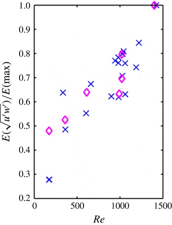
is the corresponding probability of the turbulent velocity occurring within the bolus. Figure 2 presents a comparison of the calculated expected values
 $E(u)$
of the turbulent velocities for each of the averaging methods described above. Here, the expected values are normalized by the maximum expected value observed in the data set. Due to the issue that both methods tend to produce spurious velocity fluctuations around the bolus edge, we also compared the results from both methods after we had ‘masked out’ the turbulent velocities at the bolus edge. Results from this calculation showed a slight decrease in the numerical value of the expected values, but the overall trend of the calculations for both techniques did not change with the removal of the edge velocities. Since there is no substantial difference in the results from both methods, and the overall trend of the calculations is similar, we decided to use the ensemble averaging method, with the results presented in § 3.3.1. The errors associated with the edge effects of the ensemble averaging technique are reflected in the associated error calculations.
Comparison of averaging techniques used to calculate the expected values of the turbulent velocity distributions. Symbols
 $\times$
indicate results of the ensemble averaging technique while ♢ indicate results of the spatial filtering method.

2.4 Non-dimensional parameters
To determine the importance of the system parameters on bolus generation and propagation, a set of non-dimensional parameters were used in our analysis. In these experiments, the following experimental parameters could be varied: the upper and lower layer depths
 $h_{1}$
and
 $h_{2}$
, the incident wave amplitude
 $a_{0}$
, the wave frequency
 ${\it\omega}$
, the interfacial thickness
 ${\it\delta}$
, the viscosity
 ${\it\nu}$
, the slope
 ${\it\gamma}$
and the reduced gravity
 $g^{\prime }=2g({\it\rho}_{1}-{\it\rho}_{2})/({\it\rho}_{1}+{\it\rho}_{2})$
. Using the Buckingham Pi Theorem, five dimensionless groups are formed, including a layer depth ratio
 $h_{2}/h_{1}$
, an interfacial thickness parameter
 $k{\it\delta}$
, a wave steepness parameter
 $ka_{0}$
, a wave Froude number
 $Fr={\it\omega}a_{0}/(g^{\prime }H)^{1/2}$
and a wave Reynolds number
 $Re=({\it\omega}a_{0}^{2})/{\it\nu}$
. Here,
 $H=(h_{1}h_{2})/(h_{1}+h_{2})$
so that the denominator of
 $Fr$
is the linear long wave speed for Boussinesq two-layer flow, while the numerator
 ${\it\omega}a_{0}$
reflects the overall velocities of the wave motions. The slope
 ${\it\gamma}$
is already dimensionless.
For this study, we expect the wave forcing parameters
 $Fr$
,
 $Re$
and
 $ka_{0}$
to have a significant influence on the bolus dynamics. These three parameters are used to study the dynamics of bolus propagation on the uniform slope, with a range of values for these experiments comprising of
 $Fr=(0.03{-}0.33)$
,
 $Re=(50{-}1985)$
and
 $ka_{0}=(0.03{-}0.72)$
. While the topographic slope
 ${\it\gamma}$
is also thought to strongly impact bolus formation, it was not varied in the current study. A further discussion of this issue is presented in § 4.
3 Results
We present and discuss the results of three sets of experiments. In the first set of experiments, the mechanisms for general bolus formation are qualitatively analysed using the combined techniques of PIV and PLIF. For the second set, a wide range of initial wave forcing conditions is employed by adjusting the amplitude and frequency of the incident wave train. From the results, a qualitative classification of bolus formation is developed and related to the incident wave forcing. The third set of experiments focuses on the physical characteristics of the boluses themselves. Using simultaneous measurements of the velocity and density fields, features such as the propagation speed and turbulent velocities are examined and related to the initial forcing conditions.
3.1 Bolus formation
We first take a look at general bolus formation and address the question: what are the key flow mechanisms that govern the formation of boluses? In order to capture the density and velocity fields of the flow during the bolus formation process, simultaneous PLIF/PIV measurements were obtained. Two different types of wave trains, one with low initial forcing conditions and one with relatively higher initial forcing conditions, were run over the slope to observe the difference in bolus formation. For low wave forcing conditions,
 $a_{0}=2.4~\text{cm}$
and
 ${\it\omega}=0.63~\text{rad}~\text{s}^{-1}$
(
 ${\it\lambda}=76~\text{cm}$
), leading to
 $Re=362$
and
 $Fr=0.13$
. For the higher wave forcing,
 $a_{0}=3.3~\text{cm}$
and
 ${\it\omega}=0.82~\text{rad}~\text{s}^{-1}$
(
 ${\it\lambda}=47~\text{cm}$
), resulting in
 $Re=890$
and
 $Fr=0.23$
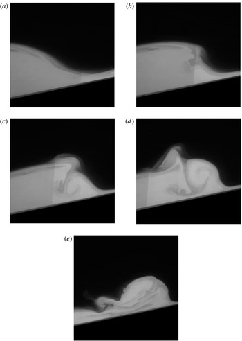
. A typical bolus formation event for relatively low forcing conditions is shown through a progression of images in figure 3. As the train of periodic waves approaches the slope, the decrease in water depth causes a gradual steepening of the wave front. The first wave of the packet typically shoals up the slope with no overturning or mixing, an observation noted by Wallace & Wilkinson (Reference Wallace and Wilkinson1988) and Helfrich (Reference Helfrich1992). As the gravitational force overcomes the forward momentum of the fluid mass, it begins to move back downslope, where it encounters the next steepening wave in the packet, as shown at the right in figure 3(a). The collision of the backflow with the forward moving wave front appears to cause a ‘stagnation point like’ feature in the front part of the steepening wave. As the wave continues forward, the downslope backflow is forced upward along the front edge of the wave, as shown in image 3(b). Dense fluid is raised, displacing less dense fluid, which contributes to the development of a counter-clockwise rotating vortex (figure 3
c). The lee of the wave, which still has forward momentum, continues to move in the upslope direction. Further on, as this fluid interacts with both the incoming backflow and the newly developed vortex, it overturns (in a ‘backward’ sense) and is quickly engulfed into the growing vortex, shown in figure 3(d). The vortex then ‘pinches off’ from the now deteriorating wave and continues to move further up the slope as a bolus (image 3
e).
Image sequence of a bolus formation event for relatively low forcing conditions. For this case,
 $Re=362$
and
 $Fr=0.13$
.

A similar bolus formation process is observed for solitary internal waves by Aghsaee et al. (Reference Aghsaee, Boegman and Lamb2010) for cases when the wave slope is much smaller than the topographic slope. Termed surging breakers, they find that a ‘separation bubble’ (our vortex) forms beneath the shoaling wave and is pushed upslope, where it becomes a turbulent bolus. This phenomenon was also noted by Michallet & Ivey (Reference Michallet and Ivey1999) for solitary waves, where a vortex formed beneath the rear face of the shoaling wave due to flow separation. Additionally, Aghsaee et al. (Reference Aghsaee, Boegman and Lamb2010) also note that the generation of each bolus is instigated by the downslope flow behind a moving bolus interacting with the next upslope surge, which is similar to our case for periodic wave trains. However, according to Helfrich (Reference Helfrich1992), the number of boluses produced was found to be dependent upon the ratio of the horizontal length scale of a solitary wave to the pycnocline depth above the slope
 $({\it\lambda}/L_{i})$
. This is different from our study, where the number of boluses produced is equal to the number of waves generated in the wave train. We attribute this difference to the physical discrepancies between shoaling sinusoidal waves versus solitary waves of depression.
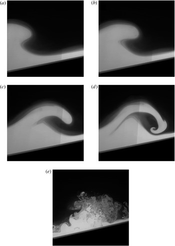
Bolus formation for the case of higher wave forcing is displayed in figure 4. In this situation, the bolus formation process is similar to that of low wave forcing conditions in the early stages (figure 4 a). However, a fundamental difference occurs as the lee of the incoming wave encounters the impeded, developing vortex within the wave front. At this point, instead of being engulfed in the developing bolus, the back of the wave is carried up and over the vortex by the excess momentum of the wave (image 4 b), creating a gravitational instability, which in turn leads to wave breaking (figure 4 c,d). The resulting turbulent fluid mass, which displays no similar characteristics in relation to the well-defined vortex presented above, is then pushed upslope by the remaining wave momentum (image 4 e). This breaking process is comparable to the plunging breaker identified by Aghsaee et al. (Reference Aghsaee, Boegman and Lamb2010) for a wave of depression, especially the occurrence of the Rayleigh–Taylor instabilities during the point of breaking.
Image sequence of a bolus formation event for relatively high forcing conditions. For this case,
 $Re=890$
and
 $Fr=0.23$
.

In their study, Aghsaee et al. (Reference Aghsaee, Boegman and Lamb2010) attribute the change in wave breaking from surging to plunging as an effect of increasing the wave slope parameter, which is defined as the ratio of the wave amplitude to the wavelength
 $(a/L_{w})$
. This parameter is directly proportional to our wave steepness parameter
 $ka_{0}$
and wave Froude number
 $Fr$
through the wave amplitude and wavelength. As such, we also observe a change in the type of wave breaking as the wave forcing is increased.
3.2 Bolus classification
The differences in bolus formation presented above allow us to formulate additional key questions regarding bolus formation. Primary among these questions is the following: how does bolus formation depend on the incident wave conditions, such as wave amplitude and frequency? To answer this question, a wide range of incident waves were generated by adjusting both the amplitude and frequency of the wave train. For these experiments, the array of variables included incident wave amplitudes of
 $a_{0}=1.0{-}5.6~\text{cm}$
and frequencies of
 ${\it\omega}=0.25{-}1.17~\text{rad}~\text{s}^{-1}$
, (
 ${\it\lambda}=27{-}255~\text{cm}$
). PLIF was employed to visualize the wave breaking and the subsequent boluses produced by the breaking event.
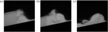
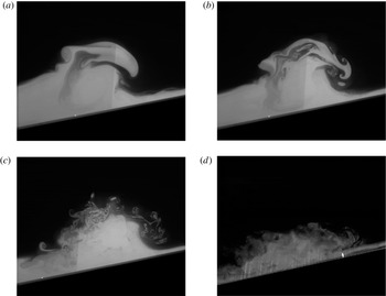
From the results, four bolus formation types were identified: backward overturning into a coherent bolus, top breaking into a turbulent bolus, top breaking into a turbulent surge and forward breaking into a turbulent surge. In each of these cases, which are depicted in figures 4–6, the major factor determining the type of formation was identified as the position of the lee end of the wave during breaking. For a backward overturning event, the lee end of the wave crest overturns in a counter-clockwise direction as it becomes engulfed in the developing vortex at the front end of the wave (figure 5 a,b). This well-formed vortex, or bolus, is then pushed further inshore by the incident wave momentum (figure 5 c). In the case of forward breaking, shown and discussed in detail in figure 4 in the previous section, the lee end of the wave has enough forward momentum to spill over the vortex forming at the wave front (figure 4 d). The forcing conditions in these cases appear to provide sufficient energy such that the front vortex begins to break up and mix, creating a more chaotic, less coherent mass of fluid which then surges up the slope (figure 4 e). In the top breaking case, shown in figure 6, the lee end of the wave attempts to pitch over the wave front (figure 6 a), yet does not have quite enough energy to do so. As a result, it breaks on the top of the developing vortex (figure 6 b). In some instances, the breaking process does not cause the vortex to completely lose its form, and produces a bolus which exhibits more turbulent characteristics but is nonetheless still fairly coherent in shape (figure 6 c). In other cases, the lee end of the wave plunges with enough force to completely break up the organized vortex. As with the forward breaking case, a more chaotic mass of fluid, which we term a turbulent surge, is created (figure 6 d) and pushed further on the slope.
Successive images of a backward breaking wave progressing into a coherent bolus.

Successive images of top breaking wave (a) and (b) into a turbulent bolus (c). In certain forcing conditions, the top breaking wave will result in a turbulent surge (d).

Classification of dominant bolus formation type in relation to wave forcing using
 $Fr$
and
 $Re$
. Symbols indicate bolus formation type: ●, backward overturning into a coherent bolus; ▿, top breaking into a turbulent bolus;

 $\times$
, forward breaking into a turbulent surge. Solid black lines are lines of constant frequency.

The prevalent bolus formation mechanism can be related to the initial wave forcing using the wave Reynolds number
 $Re$
, the wave Froude number
 $Fr$
and the wave steepness parameter
 $ka_{0}$
. Figure 7 presents the bolus formation type observed as a function of
 $Re$
and
 $Fr$
. To obtain this plot, bolus formation type was qualitatively identified by scrutinizing the location of the lee end of the wave during breaking. While there is some scatter in the results, it appears that the bolus formation type depends strongly on
 $Fr$
and more weakly on
 $Re$
. At approximately
 $Fr\geqslant 0.20$
, the wave breaking mechanism begins to deviate from backward overturning to top and forward breaking. As a result, the observed boluses are either more turbulent in nature or they are unable to form, indicating that
 $Fr\geqslant 0.20$
can be estimated as a transition point to more turbulent flow. This transition point does not seem to be captured as well by
 $Re$
, but there are no occurrences of more turbulent events for
 $Re$
less than approximately 500. The wave steepness parameter
 $ka_{0}$
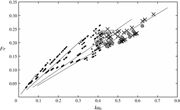
, shown in figure 8, does allow for a much clearer characterization of the transition from coherent bolus to turbulent surge. Here it can be seen that around
 $ka_{0}\approx 0.35{-}0.40$
, the primary wave breaking mechanism shifts from backward overturning to top breaking with an associated transition from coherent to turbulent boluses. As wave nonlinearity increases further and
 $ka_{0}$
exceeds
 ${\sim}0.45$
, boluses are no longer able to form and instead turbulent surges are observed. These clear shifts from more coherent to turbulent boluses, and from turbulent boluses to surges, are not captured as well by
 $Fr$
alone. Rather, the transition between formation types seems to also be dependent on the incoming wave frequency, as indicated by the lines of constant wave frequency shown in figure 8. We believe that this is because of the relationship between the time between wave events (the wave frequency) and the strength of the backflow from a previous breaking event (bolus). The association between these characteristics will have a bearing on the strength of the developing vortex at the front of the wave, which itself has a strong effect on whether the wave breaking is backward or forward. Additionally, we believe that wave steepness plays a distinct role in whether the wave breaking is top or forward. We have not fully investigated the relationship between these parameters, but the dependence of the characteristics of the boluses on the forcing frequency suggests that this dependence is strong and significant.
Classification of dominant bolus formation type in relation to wave forcing using
 $Fr$
and
 $ka_{0}$
. Symbols indicating bolus formation type are the same as those in figure 7. Solid black lines indicate lines of constant frequency.

The thickness of the interface between the fluid layers
 ${\it\delta}$
was found to also have a significant impact on bolus formation during an experiment. As a result of the continuous breaking of waves on the slope, mixing occurs at the interface and thus leads to thickening of the interface over the course of an experimental run. The effect of this on bolus formation is shown in figure 9, where
 ${\it\delta}$
is normalized by the wavenumber
 $k$
. For low forcing (low
 $Fr$
), coherent boluses form on the slope regardless of the interface thickness
 ${\it\delta}$
. For higher wave forcing
 $(Fr\geqslant 0.20)$
, bolus formation becomes more turbulent and is then non-existent for a relatively thin interface (small
 ${\it\delta}$
). As the interface begins to thicken and the parameter
 $k{\it\delta}$
exceeds a value of
 ${\sim}0.3$
, bolus-like structures of dense fluid are once again observed, even for relatively larger values of the wave forcing. It is believed that at this point, enough mixing has occurred to allow the interface to reach some kind of critical stability point. As a result, during the breaking process the lee end of the wave does not have the energy required to spill over the vortex developing at the wave front, but rather is engulfed in the flow, creating a bolus. However, as the wave frequency, and hence wavenumber, increases even further to the point where
 $k{\it\delta}>\sim 0.5$
, turbulent surges are once again observed, indicating that if the waves are forced at a high enough frequency, boluses will no longer be able to form, regardless of the interface thickness.
Bolus formation in relation to
 $Fr$
and the dimensionless interface thickness
 $k{\it\delta}$
. Symbols indicate bolus formation type: ●, backward overturning into a coherent bolus; ▿, top breaking into a turbulent bolus;

 $\times$
, forward breaking into a turbulent surge.

3.3 Bolus characteristics
We next take a closer look at the physical and dynamic characteristics of the boluses themselves to address the question: how do the characteristics of the resulting boluses depend on the initial flow conditions? To analyse bolus speed, size and turbulent velocity components during propagation, simultaneous PLIF/PIV was used to obtain two-dimensional velocity and density field measurements. For bolus speed and height calculations, wave trains of varying amplitude
 $a_{0}=1.0{-}5.6~\text{cm}$
and frequency
 ${\it\omega}=0.25{-}1.17~\text{rad}~\text{s}^{-1}$
(
 ${\it\lambda}=27{-}255~\text{cm}$
) were forced over the slope and bolus propagation after the point of breaking was observed. For turbulent Reynolds stress calculations, the amplitude was varied from
 $a_{0}=1.7{-}4.9~\text{cm}$
while the frequency was held constant at
 ${\it\omega}=0.63~\text{rad}~\text{s}^{-1}$
(
 ${\it\lambda}=76~\text{cm}$
).
3.3.1 Bolus turbulence
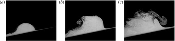
Through flow visualization, it is evident that the physical features of the resulting boluses are dependent upon the forcing characteristics of the incoming waves. Figure 10 shows PLIF images depicting the dependence of bolus shape on the strength of the wave forcing, quantified by
 $Fr$
and
 $ka_{0}$
. It is important to note that each of the boluses was produced by the backward overturning mechanism. Lower wave forcing conditions produce consistently shaped, smooth boluses like the one shown in figure 10(a), which are also similar in form to those observed by Wallace & Wilkinson (Reference Wallace and Wilkinson1988), Helfrich (Reference Helfrich1992), Michallet & Ivey (Reference Michallet and Ivey1999) and Venayagamoorthy & Fringer (Reference Venayagamoorthy and Fringer2007). However, as the wave forcing is increased, the boluses become larger, more irregular and turbulent in nature (figure 10
b,c).
PLIF images of bolus propagation on the slope for various incident amplitudes
 $a_{0}$
: (a) 1.64 cm, (b) 3.09 cm, and (c) 3.90 cm. Associated dynamic parameters are (a)
 $Fr=0.08$
;
 $ka_{0}=0.14$
, (b)
 $Fr=0.16$
;
 $ka_{0}=0.25$
, and (c)
 $Fr=0.21$
;
 $ka_{0}=0.32$
. For each case,
 ${\it\omega}=0.63~\text{rad}~\text{s}^{-1}$
,
 ${\it\gamma}=12^{\circ }$
,
 ${\rm\Delta}{\it\rho}/{\it\rho}_{0}=1\,\%$
and refractive index
 $n=1.334$
.

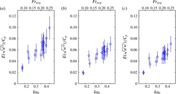
To examine this further, turbulence levels within the bolus can be quantified by measuring the turbulent velocity components as outlined in § 2.3. Figure 11 displays the expected value
 $E(u)$
of the turbulent Reynolds stress distributions (
 $u^{\prime 2}$
,
 $w^{\prime 2}$
and
 $u^{\prime }w^{\prime }$
with
 $u$
as the horizontal velocity component and
 $w$
as the vertical velocity component) for 12 bolus realizations in each set of incident wave conditions at a given location on the slope. The root mean square values of
 $u^{\prime 2}$
,
 $w^{\prime 2}$
, and
 $|u^{\prime }w^{\prime }|$
are normalized by the theoretical wave phase speed
 $C_{p}={\it\omega}/k$
so that the connection between the stresses and the magnitude of the terms driving the flows (
 $a_{0}$
for example) can be established. Each of the plots can be characterized by an initial increase in the turbulent stresses for values of
 $ka_{0}$
up to about 0.25, followed by a flatter region between values of
 $ka_{0}$
of 0.25 and 0.35 as
 $Fr$
and
 $ka_{0}$
increase. At
 $Fr\geqslant 0.2$
and
 $ka_{0}\geqslant 0.35$
, the turbulent stresses increase again (albeit somewhat weakly), indicating some kind of transition in the characteristics of the bolus. We note from previous figures that for values of
 $ka_{0}\geqslant 0.4$
the boluses exhibited turbulent characteristics or were broken up into turbulent surges.
Expected values of turbulent Reynolds stress distributions in relation to wave steepness
 $ka_{0}$
and wave Froude number
 $Fr$
.

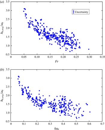
Average bolus height on slope
 $h_{b,avg}$
normalized by incident amplitude
 $a_{0}$
in relation to (a) the wave Froude number
 $Fr$
and (b) the wave steepness
 $ka_{0}$
.

3.3.2 Bolus height
Bolus size and shape depend on the magnitude of the initial wave forcing, as shown in figure 10 in the previous section. To quantify this relationship, the average bolus height on the slope was calculated and related to the incident forcing conditions. Using PLIF images, the bolus height was calculated by determining the distance between the slope and the highest point of the bolus, as defined by the location of the fluid interface. The average bolus height was then obtained by time averaging the bolus heights calculated for the entire recorded propagation period of the bolus. We note that the height of the bolus tended to decrease as the bolus moved up the slope, similar to the observation of Wallace & Wilkinson (Reference Wallace and Wilkinson1988). Figure 12 presents the average bolus height
 $h_{b,avg}$
normalized by the incident wave amplitude
 $a_{0}$
as a function of (a) the wave Froude number
 $Fr$
and (b) the wave steepness
 $ka_{0}$
. Here it is shown that as wave forcing increases, specifically the wave frequency, the average bolus height decreases. This result can be directly related to the distance of propagation. During the experiments, it was observed that the longer waves generated boluses that travelled further on the slope. As the wave frequency, which is related to the wavenumber
 $k$
through the dispersion relation, increases, more energy is diverted into the production of turbulence instead of forward propagation, causing the bolus to travel a shorter distance and dissipate at a faster rate. Because of this, the average bolus height for waves with a higher frequency is lower. The spread in the data for increased
 $Fr$
and
 $ka_{0}$
conditions can be attributed to the method of calculating bolus height for cases where the overall bolus shape is more turbulent.
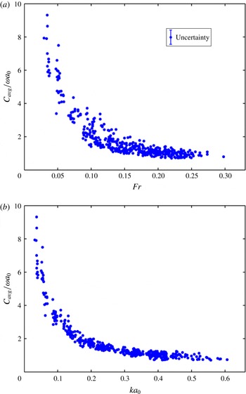
Relationship between average bolus speed on the slope
 $C_{avg}$
(normalized by
 ${\it\omega}a_{0}$
) and (a) wave Froude number
 $Fr$
, (b) wave steepness
 $ka_{0}$
.

3.3.3 Bolus speed
The relation of bolus speed to forcing is shown in figure 13. The average bolus speed on the slope
 $C_{avg}$
, normalized by the characteristic wave velocity of the incoming wave
 ${\it\omega}a_{0}$
, is shown as a function of both (a) the Froude number
 $Fr$
and (b) the wave steepness
 $ka_{0}$
. In both cases, the bolus speed is shown to decrease as the wave nonlinearity increases, yet the data seems to collapse slightly better with the
 $ka_{0}$
relationship. Starting at the lower end of wave forcing, the normalized bolus speed at first decreases dramatically, then declines at a slower rate with increased forcing. This suggests that as wave forcing increases, some of the incoming bolus energy may be shifted from forward propagation to the production of turbulence. Additionally, as the bolus boundaries become more irregular, more drag is created at the bolus edge, leading to a decrease in forward propagation. At the point where
 $Fr\geqslant 0.2$
and
 $ka_{0}\geqslant 0.35$
, the bolus speed seems to asymptote to a value equivalent to the characteristic velocity scale, for this study,
 ${\it\omega}a_{0}$
, chosen because it typically characterizes the velocity field within a wave. This change indicates a possible point of wave forcing in which the generated boluses transition to more turbulent flow, a conclusion which matches that drawn in § 3.3.1.
Venayagamoorthy & Fringer (Reference Venayagamoorthy and Fringer2007) noted that boluses may propagate similarly to gravity currents for the case of boluses propagating on a shelf break in a linearly stratified fluid. To make a comparison, we define a bolus Froude number
 $Fr_{b}={\it\omega}a_{0}/(g^{\prime }h_{b,avg})^{1/2}$
, where
 $h_{b,avg}$
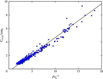
is the average bolus height on slope. This definition is similar to a Froude number used by Britter & Simpson (Reference Britter and Simpson1978), where the channel depth was replaced by the approximate gravity current height. Figure 14 presents the average bolus speed on the slope
 $C_{avg}$
in relation to the inverse of
 $Fr_{b}$
. Using this parameterization, it is evident that there a linear relationship between
 $C_{avg}$
and
 $(g^{\prime }h_{b,avg})^{1/2}$
, with a slope of approximately
 $1/2$
. While the non-dimensional bolus speed
 $(C_{avg}/{\it\omega}a_{0})$
and
 $Fr_{b}^{-1}$
both contain
 ${\it\omega}a_{0}$
in their respective denominators,
 $Fr_{b}^{-1}$
also includes the average height of the bolus,
 $h_{b,avg}$
, which varies strongly with the characteristics of the different types of boluses observed in this study.
Relationship between average bolus speed on slope
 $C_{avg}$
(normalized by
 ${\it\omega}a_{0}$
) and
 $Fr_{b}^{-1}$
. The solid line has a slope of
 $1/2$
.

Interestingly, the relationship shown in figure 14 has a similar form to the front speed derived by Benjamin (Reference Benjamin1968) for an energy-conserving boundary gravity current, where the front propagation speed
 $U=(\sqrt{g^{\prime }H})/2$
. However, it is important to note that
 $H$
is defined by Benjamin (Reference Benjamin1968) as the total channel depth and not the height of the gravity current. Moreover, Britter and Simpson found that the coefficient was a strong function of the ratio of the gravity current height and the channel height, varying from 1.0 to 2.25. Furthermore, we would not expect a bolus propagating up an inclined slope to have the same Froude number as a gravity current moving across a flat surface due to the differences in the flow dynamics. Given all of this, the similar form of our result with that of Benjamin (Reference Benjamin1968) cannot be established with more certainty with our existing data, and will need further investigation.
4 Conclusions
Laboratory experiments have been used to study the formation and propagation of internal boluses from the shoaling of progressive interfacial wave trains on a uniform slope. Four bolus formation characterizations were identified: backward overturning into a coherent bolus, top breaking into a turbulent bolus, top breaking into a turbulent surge and forward breaking into a turbulent surge. The dominance of a particular formation mechanism was shown to be dependent on the initial forcing conditions of the wave train, including the wave frequency and amplitude.
During the initial process of formation, the backflow of the previous shoaling wave was shown to interact with the overturning front edge of the incoming wave, leading to the development of a positively rotating vortex surge with substantial engulfment of the backflow. For lower forcing conditions, the back part of the wave, which continues to have forward momentum, is obstructed and engulfed into the newly developed bolus. However, for conditions in which the wave steepness parameter
 ${\sim}0.40<ka_{0}<\sim 0.45$
, the back end of the wave tends to break on the top of the front vortex, leading to the development of a more turbulent bolus. As wave forcing increases further and
 $ka_{0}$
exceeds a value of approximately 0.45, bolus formation is no longer possible and turbulent surges of dense water were observed.
The characteristics of bolus propagation were also examined in relation to the initial wave forcing. Bolus celerity was shown to decrease for increasing
 $Fr$
and
 $ka_{0}$
up to values of 0.2 and 0.3, respectively. At wave forcing conditions higher than this point, the average bolus speed asymptotes to the characteristic velocity scale
 ${\it\omega}a_{0}$
. Additionally, the normalized expected values of the turbulent Reynolds stress distributions were shown to increase above the threshold
 $Fr>0.2$
and
 $ka_{0}>0.4$
. These results thus indicate that the values of
 $Fr\approx 0.2$
and
 $ka_{0}\approx 0.3{-}0.4$
are a potential threshold for a transition to more turbulent flow.
In this study, a constant topographic slope was employed. While internal wave breaking on slopes is highly dependent on the degree of incline, we believe that the changes in bolus formation linked to slope degree can be inferred from the conclusions drawn by previously conducted experiments. Helfrich (Reference Helfrich1992) noted that as the slope decreased, the overturning of the breaking wave was not as intense, and that the point of initial breaking occurred further offshore so that the breaking process took place over a longer distance. Both of these conclusions were also made by Michallet & Ivey (Reference Michallet and Ivey1999). Additionally, the results of Aghsaee et al. (Reference Aghsaee, Boegman and Lamb2010) indicate that in order to achieve the same shoaling mechanism on a shallower slope, a larger wave forcing is required. Drawing on these conclusions, we believe that on shallower slopes, backward breaking waves will be the dominant shoaling mechanism, leading to the formation of coherent boluses, as evidenced by the observations of Wallace & Wilkinson (Reference Wallace and Wilkinson1988). Transition to a different breaking type, such as top or forward breaking, will also require a higher level of wave forcing than shown in this current study. However, to quantitatively determine these changes, future work will address the effect of the topographic slope on bolus propagation. Resulting flow variations can then be related to the changes in topography and forcing through the use of the internal Iribarren number (the ratio of the boundary slope to the wave slope), as employed by Boegman et al. (Reference Boegman, Ivey and Imberger2005) and Aghsaee et al. (Reference Aghsaee, Boegman and Lamb2010).
Acknowledgements
This research was supported by a National Science Foundation Graduate Research Fellowship for C.D.M., as well as the National Science Foundation Fluid Dynamics program under grant no. CBET 1133380. The authors would also like to thank Thomas Peacock for his contribution and insight to the formation of internal boluses.