


1. Introduction
In plants, the epidermis plays a central role in growth, development and environmental adaptation (Javelle et al., Reference Javelle, Vernoud, Rogowsky and Ingram2011). Acting as the outermost protective layer, it regulates exchanges between internal tissues and the external environment (Samuels et al., Reference Samuels, Kunst and Jetter2008) while providing mechanical support channelling growth and development (Galletti et al., Reference Galletti, Verger, Hamant and Ingram2016). In aerial organs, the epidermis experiences substantial mechanical stress due to the differential growth rates of underlying tissues (Kutschera & Niklas, Reference Kutschera and Niklas2007). As a result, epidermal cells are continuously stretched and are at risk of rupturing or separating if their cell wall properties and intercellular adhesion are not properly maintained (Asaoka et al., Reference Asaoka, Ooe, Gunji, Milani, Runel, Horiguchi, Hamant, Sawa, Tsukaya and Ferjani2021; Verger et al., Reference Verger, Long, Boudaoud and Hamant2018). Preserving epidermal integrity is therefore essential for normal plant growth and survival.
Understanding the mechanisms that maintain epidermal integrity has become a key question in plant developmental biology. Previous studies have identified several mutants affecting molecular regulators of epidermal integrity, with defects specifically targeting adhesion (Baba & Verger, Reference Baba and Verger2024) and cellular integrity (Harnvanichvech & Long, Reference Harnvanichvech and Long2025). For example, the pectin-deficient mutant quasimodo2 (qua2) displays severe epidermal adhesion defects, resulting in impaired growth, development and increased sensitivity to drought (Mouille et al., Reference Mouille, Ralet, Cavelier, Eland, Effroy, Hématy, McCartney, Truong, Gaudon, Thibault, Marchant and Höfte2007; Raggi et al., Reference Raggi, Ferrarini, Delledonne, Dunand, Ranocha, de Lorenzo, Cervone and Ferrari2015; Verger et al., Reference Verger, Liu and Hamant2019). Other mutants, such as actin-related protein2 (arp2), which is defective in actin nucleation, show comparatively mild adhesion defects (Erguvan et al., Reference Erguvan, Heymans, Atakhani, Gascon, Smith, Ali and Verger2025; Le et al., Reference Le, El-Assal, Basu, Saad and Szymanski2003; Li et al., Reference Li, Blanchoin, Yang and Lord2003).
The epidermis is also covered by a cuticle that acts as a barrier to the environment and ensures controlled gas exchange through stomata (Samuels et al., Reference Samuels, Kunst and Jetter2008). Mutants with impaired cuticle formation often exhibit increased epidermal permeability, abnormal organ fusion and reduced resistance to environmental stress (Ingram & Nawrath, Reference Ingram and Nawrath2017). Although the processes governing cell adhesion, cuticle deposition and wall integrity are increasingly understood, many key regulatory components remain unknown.
Typical manifestations of epidermal integrity defects include cell bursting, loss of intercellular adhesion and cuticular permeability. These phenotypes are often visually detectable using microscopy (Buda et al., Reference Buda, Isaacson, Matas, Paolillo and Rose2009; Verger et al., Reference Verger, Cerutti and Hamant2018) or dye-penetration assays (Tanaka et al., Reference Tanaka, Tanaka, Machida, Watanabe and Machida2004), yet reliably quantifying their severity remains challenging. For example, adhesion defects can be observed using confocal microscopy combined with cell wall staining (Verger et al., Reference Verger, Cerutti and Hamant2018), but the heterogeneous distribution, size and appearance of adhesion defects across tissues, makes large-scale quantification challenging.
One robust approach to evaluate epidermal permeability relies on the penetration of hydrophilic, cell wall-binding dyes through the epidermis. In intact tissues, the cuticle acts as a barrier preventing dye penetration (Figure 1a). Conversely, if epidermal cells are damaged, separated, or if the cuticle is compromised, the dyes infiltrate and bind to the cell walls (Figure 1b). Two commonly used dyes are Toluidine Blue (TB) and Ruthenium Red (RR), both of which are thought to preferentially bind de-esterified pectins, although TB can also interact with cellulose and lignin, producing distinct staining patterns (Piccinini et al., Reference Piccinini, Nirina Ramamonjy and Ursache2024). Traditionally, RR and TB staining have been used to assess epidermal defects in a qualitative manner (Kohorn et al., Reference Kohorn, Zorensky, Dexter-Meldrum, Chabout, Mouille and Kohorn2021; Tanaka et al., Reference Tanaka, Tanaka, Machida, Watanabe and Machida2004), but mutants with different defect severities often display noticeably different staining intensities, suggesting that a quantitative approach could provide a more precise comparison between genotypes (Kohorn et al., Reference Kohorn, Zorensky, Dexter-Meldrum, Chabout, Mouille and Kohorn2021.
Epidermal permeability assessment using penetration assay. Note: A hydrophilic penetrating cell wall binding dye, here ruthenium red (RR in the figure), is used to stain the seedings. Depending on the state of the cuticle and the epidermis of the sample, the dye may penetrate and stain the cell wall. Both the cellular and seedling scales are presented. (a) Without cuticle defects, the dye is unable to penetrate the tissue. The hypocotyl of the sample is not stained. Root may uptake the dye and become red in the case of RR staining. (b) If the sample presents cuticle defects, dead epidermal cells or cell adhesion defects, the dye can penetrate and stain the cell wall. The intensity of the colouration is correlated to the level of dye penetration.

Figure 1. Long description
The diagram is divided into two main sections: Cellular Scale and Seedling.
Panel A, labeled No defect, shows a healthy plant surface. At the Cellular Scale, a solid yellow Cuticle layer sits atop the Epidermis cells. A black arrow points to the Cell wall. A droplet labeled R R (Ruthenium Red) bounces off the cuticle, indicating no penetration. On the right, the Seedling is white with only the root tip stained red.
Panel B illustrates three types of defects.
1. Cuticle defect: The yellow cuticle is fragmented. The R R droplet penetrates between cells, staining the cell walls dark red. The corresponding seedling shows Low penetration with a light pink hypocotyl.
2. Cell death: A gap exists where an epidermal cell is missing, shown by a dashed outline. The R R droplet enters this void.
3. Cell adhesion defect: A physical gap between two epidermal cells allows the R R droplet to pass through.
The bottom-most seedling represents High penetration, where the entire hypocotyl is stained a deep dark red.
It is possible to quantify TB staining by extracting the dye from tissues after washing and measuring absorbance spectrophotometrically (Xing et al., Reference Xing, Creff, Waters, Tanaka, Goodrich and Ingram2013). However, this approach is limited, as variations in tissue size and total absorption capacity could introduce substantial bias unrelated to epidermal defects. A more robust strategy would involve quantifying relative staining intensity directly from imaging data. While RR and TB staining are widely used in plant biology, no standardised workflow currently exists for sample preparation, image acquisition and quantitative image analysis to reliably compare epidermal defects across genotypes and experimental conditions.
Here, we present RRQuant, a standardised, high-throughput workflow for the quantitative characterisation of epidermal integrity defects in seedlings. This pipeline integrates standardised sample preparation, high-throughput imaging and semi-automated image processing using deep learning–based tissue segmentation. Quantitative features, including staining intensity and morphological traits, are extracted using a streamlined ImageJ-based workflow and analysed via an integrated R-based script and R Shiny application. By combining automation with flexibility, RRQuant enables reproducible, large-scale comparisons of epidermal defects across mutants, transgenic lines and wild-type controls. Our aim is to provide the community with an open, accessible platform that bridges the gap between qualitative assessment and quantitative, standardised phenotyping of epidermal integrity. All macros, trained models, supporting scripts and the shiny app are available at github.com/VergerLab/RRQuant, along with a detailed protocol for both wet lab and computing workflows.
2. Results and discussion
2.1. Considerations for standardised sample preparation and high-throughput imaging
To establish a robust and reproducible workflow for quantifying epidermal integrity defects, we first optimised sample selection, staining conditions and imaging strategies (Figure 1).
2.1.1. Choice of organ and growth conditions
We selected etiolated (dark-grown) hypocotyls as the standard organ for RRQuant because they display the most pronounced epidermal adhesion defects (Verger et al., Reference Verger, Long, Boudaoud and Hamant2018). Hypocotyls grown in darkness undergo rapid, anisotropic elongation, resulting in high longitudinal tension on the epidermis, which tends to amplify defects such as cell separation, cuticular damage or cell bursting (Malivert et al., Reference Malivert, Erguvan, Chevallier, Dehem, Friaud, Liu, Martin, Peyraud, Hamant and Verger2021; Verger et al., Reference Verger, Long, Boudaoud and Hamant2018). Another consideration was that light-grown seedlings accumulate pigments such as chlorophyll and sometimes anthocyanins under stress, which can interfere with dye-based staining and imaging (Figure 2a). Working with dark-grown seedlings therefore provides both clearer visualisation and greater sensitivity for detecting epidermal integrity defects.
Samples, dyes and imaging. Note: (a) Light- vs. dark-grown seedlings. Left: Seedling grown in the light on a liquid medium containing 3% sucrose, showing chlorophyll pigments (green) and anthocyanin (purple; sign of stress). Right: Dark-grown seedling on solid medium, without sucrose, showing a clear (white) elongated hypocotyl and faint yellow pigmentation in the small cotyledons. (b) Effect of staining duration on the qua2-1 mutant. Left: Non stained. Middle: Stained for 1 min with ruthenium red. Right: Stained for 30 minutes. C-E Comparison of imaging mode and dye. Note the same samples have been imaged under different conditions. Col-0 and qua2-1 were either non stained (NS), stained with RR or TB imaged in Brightfield (BF) Transmission (c), Brightfield Epi-illumination (d) or Darkfield (e). (f) Illustration of sample staining procedure: Dark-grown hypocotyls are grown on a medium of choice. Some samples are stained with 0.05%RR, rinsed and placed on the agarose plate, while others are directly placed for imaging without staining. Several mutants, conditions or treatments can be compared with WT control. Illustration of high-throughput imaging, making use of tile scanning function to acquire a large number of samples at once. Scale bars: 1 mm.
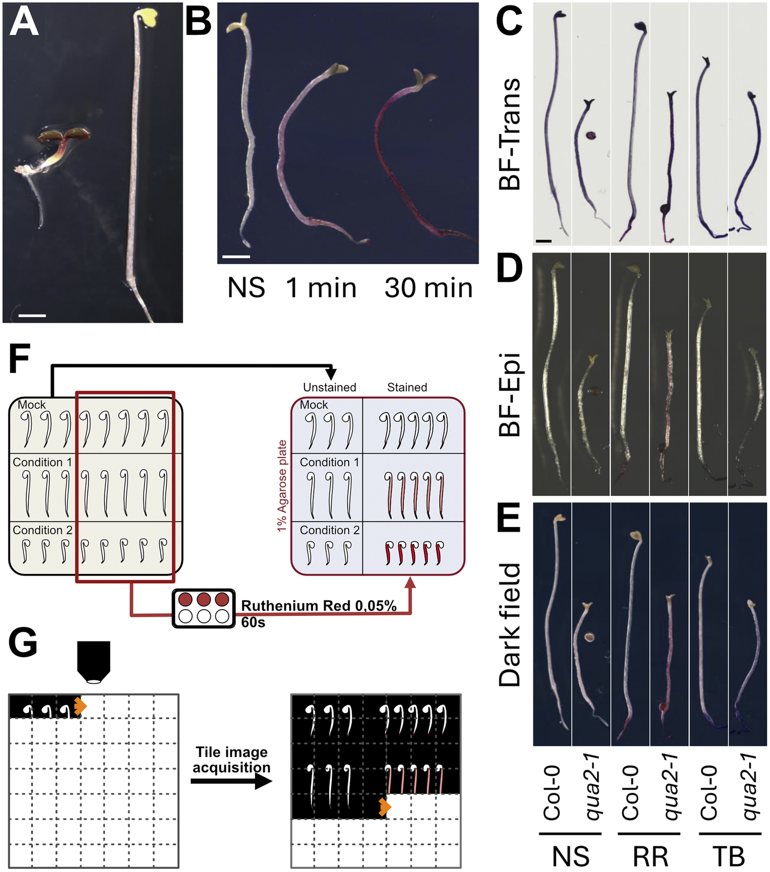
Figure 2. Long description
Panel A: Two photos of seedlings. The left seedling is short with green and purple leaves. The right seedling is much taller with a white elongated hypocotyl and yellow cotyledons. Scale bar is 1 mm.
Panel B: Three seedlings labeled N S, 1 min, and 30 min. The (Non stained) seedling is white. The 1 min seedling shows light pink staining. The 30 min seedling is dark purple.
Panels C, D, and E: A grid comparing Col-0 and qua 2-1 mutants across three imaging modes: (BrightField)-Trans (C), B F-Epi (D), and Dark field (E). Each mode shows six seedlings grouped by staining: N S (non-stained), R R (Ruthenium Red), and T B (Toluidine Blue). Col-0 seedlings are consistently longer than qua 2-1. R R and T B stains appear as dark outlines or solid colors depending on the imaging mode.
Panel F: A flowchart diagram. On the left, a grid of seedlings labeled Mock, Condition 1, and Condition 2. A red box selects a subset of seedlings which are routed through a staining step with Ruthenium Red 0.05 percent for 60 s. On the right, the final 1 percent Agarose plate shows Unstained and Stained seedlings side-by-side.
Panel G: A diagram of tile image acquisition. A microscope objective moves across a grid, capturing individual seedling images. An arrow points to the resulting composite image where multiple seedling tiles are stitched together.
2.1.2. Choice of staining dye
We next compared RR and TB, two widely used dyes for assessing epidermal permeability (Piccinini et al., Reference Piccinini, Nirina Ramamonjy and Ursache2024) (Figure 2c–e). Both dyes are thought to bind de-esterified pectins, although TB also binds cellulose and lignin, producing blue to purple hues depending on the tissue composition (Piccinini et al., Reference Piccinini, Nirina Ramamonjy and Ursache2024). While TB staining can be informative, RR provided sharper contrast under most imaging conditions and was easier to distinguish from background pigmentation (see next sections). For these reasons, RR was selected as the default dye for the RRQuant workflow.
2.1.3. Optimisation of imaging mode
We tested several imaging approaches to identify the best setup for quantifying staining intensity, including transmission brightfield, epi-brightfield and darkfield illumination (Figure 2c-e). In transmission mode, highly pigmented or opaque tissues appeared darker, reducing the apparent colour saturation and complicating quantification (Figure 2c). Epi-brightfield imaging improved contrast but introduced reflection artefacts from the sample surface (Figure 2d). In contrast, darkfield illumination produced the most vibrant and consistent colouration of RR-stained tissues, offering optimal sensitivity for quantification (Figure 2e). However, the oblique illumination caused the gel background to appear slightly blue rather than black (Figure 2e), which further influenced the choice of RR over TB as the dye of choice.
Optimisation of gel substrate: Because seedlings with epidermal defects are highly prone to dehydration after staining, we optimised the support medium used during imaging. We compared agar and agarose gels at different concentrations and thicknesses. We found that 1% agarose provided a homogeneous, transparent and stable surface for sample placement, while standard agar produced a yellowish background and stronger optical heterogeneity, which reduced image quality. For all experiments, seedlings were therefore placed on 12 cm square plates filled with 50 mL of 1% agarose gel to ensure consistent hydration and optimal imaging conditions.
2.1.4. Effect of staining duration
We next tested whether the duration of RR staining would influence staining intensity or if staining somehow plateaus very early on. We stained qua2-1 for 1 minute or 30 minutes in parallel with no staining (Figure 2b) and found that staining time had a clear influence on the staining intensity. Thus, it is important to first assess the ideal staining time required for the experiment depending on the samples used and the imaging conditions, as well as to properly standardise staining time between samples to avoid variation dues to different exposure time to staining (see also Supplementary Figure S1).
2.1.5. Standardised sample preparation workflow
Based on these optimisations, we established a standardised preparation procedure (Figure 2f). Four-day-old dark-grown seedlings are stained in 0.05% RR for a predefined duration (depending on genotypes used and growth conditions; see Supplementary Figure S1) and rinsed briefly. For each genotype, 3–5 unstained seedlings are prepared as negative controls alongside 20–25 stained seedlings (Figure 2f,g). Samples are then arranged manually on hydrated 1% agarose plates and imaged using a stereo microscope equipped with a colour camera, a motorised stage and darkfield illumination. Tile-scan imaging allows the capture of entire plates at high resolution, producing large stitched RGB TIFF images that serve as input for downstream image segmentation and quantification (Figure 2f).
2.2. Deep learning-based hypocotyl segmentation
A central component of the RRQuant workflow is the ability to precisely measure RR staining intensity specifically within the hypocotyl region while excluding cotyledons, roots, seed coats and background artefacts. While manual delineation of hypocotyl boundaries in images is possible, it is highly time-consuming and introduces user bias, which limits reproducibility, especially in high-throughput experiments. In preliminary tests, classical image processing methods, such as simple thresholding or more advanced machine learning–based pixel classification, also failed to achieve satisfactory segmentation accuracy, particularly in separating hypocotyls from roots where staining intensity and morphology are highly similar. To overcome these limitations, we implemented a deep learning–based segmentation approach using the RootPainter platform (Smith et al., Reference Smith, Han, Petersen, Olsen, Giese, Athmann, Dresbøll and Thorup-Kristensen2022). RootPainter uses a modified U-Net convolutional neural network (CNN) architecture, enabling efficient segmentation through an interactive, corrective annotation strategy. This approach allowed us to iteratively improve the model performance by continuously updating the training dataset with human-corrected predictions.
To generate a robust and generalisable RootPainter hypocotyl segmentation model, we adopted an iterative training process with successive model versions (V0, V1 and V2). To reduce user-specific bias, multiple annotators collaboratively generated ground-truth masks. While early iterations (V0, V1) were trained on smaller datasets, the final V2 model was trained on a significantly expanded and diverse dataset which was first segmented by the V1 model and manually corrected, to maximise robustness across varying genotypes and experimental conditions (see Methods).
We evaluated the three model iterations (V0, V1 and V2) on a validation dataset with manually annotated ground-truth masks. Model V2 achieved the highest performance across all metrics, with an F1 score of 0.976 and an IoU score of 0.952. Compared to the baseline (V0), V2 reduced False positives by approximately 44% and False negatives by 50%, indicating a significantly more robust detection in the latter iteration. This quantitative improvement translates to significantly more robust detection in complex segmentation scenarios (Figure 3). While V0 frequently exhibited fragmented segmentation masks with large patches of missing tissue (Figure 3a, left panels), V2 was more reliable in generating continuous masks that accurately spanned the entire hypocotyl region. Moreover, V2 demonstrated superior boundary definition, particularly at the root–hypocotyl junction, successfully excluding root tissue (Figure 3a, right panels). The high precision (0.983) of the V2 model demonstrates high reliability and ensures that identified pixels are true hypocotyl tissue.
Qualitative and quantitative improvement of hypocotyl segmentation. Note: (a) Visual comparison of segmentation masks generated by the baseline RootPainter model (V0) and the final model (V2). V2 demonstrates improved continuity in the hypocotyl region (left, green arrows) and accurate exclusion of root tissue at the basal boundary (right, green arrow) compared to V0. (b) Performance metrics for all model iterations on an independent validation set. V2 outperforms previous versions across all metrics, showing significant reductions in both False positives (Fp) and False negatives (Fn).

Figure 3. Long description
Panel A contains four vertical photographs of plant hypocotyls with overlaid segmentation masks. The first pair shows V 0 with fragmented red and blue masks, while V 2 shows a continuous blue mask indicated by two green arrows pointing to the stem. The second pair shows V 0 including root tissue in the mask, while V 2 correctly excludes it, indicated by a green arrow at the basal boundary. Scale bars are present at the bottom of the images.
Panel B is a performance metric table with seven columns: Model, F 1 Score, I o U (Jaccard), Precision, Recall, T p (Count), F p (Count), and F n (Count).
Data for V 0: F 1 Score 0.952, I o U 0.909, Precision 0.968, Recall 0.937, T p 5 754 527, F p 190 057, F n 389 403.
Data for V 1: F 1 Score 0.933, I o U 0.874, Precision 0.961, Recall 0.906, T p 5 566 013, F p 223 181, F n 577 917.
Data for V 2: F 1 Score 0.976, I o U 0.952, Precision 0.983, Recall 0.968, T p 5 950 060, F p 105 525, F n 193 87.
Interestingly, model V1 showed a regression compared to V0, with the F1 score dropping to 0.933. This degradation came primarily from a substantial increase in False negatives, resulting in a recall of only 0.906, the lowest of the three models. This degradation likely arose due to overfitting specific phenotypes during training, leading to a more specialised (and less general) model.
The trained V2 model can now be used as a baseline segmentation model in the RRQuant workflow. We expect that the model’s performance can be further enhanced as more annotated data becomes available. Note that the model V2 we provide here is likely overfitted to the type of images generated by the microscope primarily used in this study (Supplementary Figure S2). Yet, because RootPainter supports incremental training, users can easily fine-tune this model to their own experimental setups, such as different microscopes, dyes or even entirely different organs.
2.3. Computational workflow: Image processing and quantification
We then developed an image processing pipeline that enables high-throughput, standardised and reproducible quantification of epidermal integrity defects from RR-stained seedlings (Figure 2). The pipeline was designed to process large, stitched images generated from tile scans, automatically segment the hypocotyls and extract quantitative features such as RR staining intensity and hypocotyl length. To make it accessible to a wide range of users, we developed an ImageJ-based toolset that combines semi-automated image pre-processing with guided manual corrections of deep learning-based segmentation as well as batch quantification. All steps are standardised to ensure that results are directly comparable across genotypes, experiments and laboratories.
2.3.1. Image splitting and standardised naming
Large plate images containing multiple genotypes and both stained and unstained controls (Figure 2f) are first processed using a dedicated ImageJ macro. Users select regions of interest corresponding to each sample set (e.g., Col-0 unstained, qua2-1 stained), assign genotype names (or specific growth conditions) and replicate numbers and save individual TIFF images. This macro automatically generates a consistent file-naming scheme, which is essential for batch processing and downstream analysis (Figure 4a).
Image processing. Note: (a) File preparation: Image splitting and standardised naming using RRQuant toolset in ImageJ (or Fiji; Split Img). (b) Hypocotyl segmentation: images are segmented using RootPainter trained model. The masks can be corrected using RRQuant toolset in ImageJ (Mask Corr). (c) Quantification of the colour intensity of RR and morphological measurements using RRQuant function of the toolset. (d) Analysis is conducted with an R script to combine, organise the data and perform statistical analysis. (e) Data visualisation is facilitated using RRQuant Shiny app (in R) to display plots and verify data accuracy using interactive plots.

Figure 4. Long description
The flowchart is divided into five sections.
* Panel A, File preparation: Large tiles T I F F images are processed through an Image J macro. A grid of seedling images is split and named into categories: W T-NonStained, W T-Stained, c 1-NonStained, c 1-Stained, c 2-NonStained, and c 2-Stained.
* Panel B, Segmentation: A seedling image is processed using RootPainter. An arrow points to a segmented blue mask of the hypocotyl. A second arrow labeled Mask correction with a paintbrush icon points to a refined, clean blue mask in Image J.
* Panel C, Quantification: An Image J macro processes the masks to generate two data stacks: Morphometry (blue tables) and Staining intensity (red tables).
* Panel D, Analysis: Data from the tables are fed into an R script, indicated by the R logo. This yields a Master data table with purple headers.
* Panel E, Visualization: The master data is processed through an R Shiny app. The final output is a graphical user interface titled R R Quant: plot your data, featuring a violin plot showing Length on the y-axis for three different sample groups.
2.3.2. Hypocotyl segmentation
The cropped images are segmented using the trained RootPainter model, which produces binary masks for hypocotyl regions. Because the segmentation is not always perfect, a second ImageJ macro facilitates manual corrections of the predicted masks while displaying the original image as a reference. This combination of automated segmentation and targeted corrections balances accuracy with efficiency and ensures reproducibility between users (Figure 4b).
2.3.3. Staining intensity and morphometric quantification
Once the corrected masks are finalised, a third macro quantifies RR staining intensity together with basic hypocotyl morphometrics using the MorphoLibJ plugin (Legland et al., Reference Legland, Arganda-Carreras and Andrey2016). To capture staining intensity, we implemented a custom approach based on the HSB colour space. The RGB images are converted into Hue, Saturation, and Brightness components. The Brightness channel is inverted, and an Intensity image is computed by summing the inverted Brightness and Saturation signals. The average intensity within each segmented hypocotyl is extracted as the primary quantitative measure. To reduce potential edge artefacts caused by bright halos or incomplete mask boundaries, intensity is calculated within an eroded region (−10 px) of each hypocotyl mask. In parallel, hypocotyl length is extracted from the corrected segmented masks (not the eroded version). Length is derived from the geodesic diameter (accounts for hypocotyl curvature), and other shape descriptors can be optionally included for downstream analysis (e.g., average thickness, tortuosity, surface area, etc. See MorpholibJ plugin) (Figure 4c).
2.4. Computational workflow: Data analysis and visualisation
Next, we implemented the data analysis pipeline, which transforms raw image-derived measurements into interpretable quantitative comparisons between genotypes and conditions. To make this process both standardised and accessible, we developed an R-based analysis toolkit coupled with an interactive Shiny application (Figure 4d,e).
2.4.1. Data aggregation, normalisation and statistics
The image processing pipeline produces quantitative measurements of RR staining intensity and hypocotyl morphology for each sample. These measurements are automatically combined into a single data table where each row represents one seedling, and metadata such as genotype, staining condition and replicate number are stored alongside the quantitative values. To correct for experimental variability, RR staining intensity is expressed relative to internal controls. For each genotype, we normalise stained samples to the mean intensity of non-stained seedlings grown under the same conditions. This approach accounts for differences in background intensity, sample size and imaging conditions, enabling direct comparisons across experiments. To assess differences between genotypes or treatments, the analysis pipeline applies statistical tests directly within R (Figure 4d).
2.4.2. Visualisation and interactive data exploration
To make the analysis user-friendly, we developed a companion R Shiny app that integrates visualisation and quality control tools. The app provides customisable plots (choose which genotypes, treatments, and replicates to display), interactive data inspection (hovering over individual points reveals sample-specific metadata) and outlier detection (outlier data points can be traced back to their corresponding raw images to verify whether they represent genuine biological variation or segmentation artefacts). This interactive design ensures that users can validate data quality at every step of the workflow, even when dealing with high amount of data, while also generating publication-ready figures directly from the app (Figure 4e).
2.5. RRQuant reveals quantitative differences in epidermal defect intensity between adhesion defective genotypes
Finally, we assessed the usefulness of our approach in resolving quantitative differences between adhesion defective genotypes. Different mutants have previously been shown to have different level of adhesion defect severity, but the severity of the phenotypes were only compared qualitatively (e.g. (Kohorn et al., Reference Kohorn, Zorensky, Dexter-Meldrum, Chabout, Mouille and Kohorn2021; Verger et al., Reference Verger, Chabout, Gineau and Mouille2016). Here we first used the mutant lines arp2-1 (very mild) and qua2-1 (severe) stained for only 1 minute. Our quantification shows a clear quantitative difference consistent over three biological replicates, matching the previously described severity of the phenotypes. With such short staining duration, the relative staining intensity for arp2-1 (1.034 with standard deviation 0.033) was undistinguishable from Col-0 (1.028±0.036), both on images (Figure 5a) and as quantified by RRQuant (Figure 5b). On the other hand, qua2-1 showed a clear staining (Figure 5a) and significant increase in relative staining (1.147±0.075; Figure 5b). In addition to staining intensity, the workflow outputs several morphometric measurements. Here, the RRQuant pipeline confirmed that the qua2-1 mutant hypocotyls are shorter (Verger et al., Reference Verger, Chabout, Gineau and Mouille2016; Figure 5c) but also unveiled that they are thinner (Figure 5d) and more tortuous (overall waviness of the hypocotyl, Figure 5e). Specifically, qua2-1 showed a significantly decreased length (6.98±1.34mm) compared to Col-0 (12.66±2.00mm) and arp2-1 (12.29±2.07mm). qua2-1 was also significantly thinner (213.09±16.87μm) compared to Col-0 (226.95±13.64μm) and arp2-1 (227.22±13.24μm). Finally, it was also slightly but significantly more tortuous (1.089±0.127) than Col-0 (1.019±0.015) and arp2-1 (1.037±0.026). To further test the sensitivity of our approach for staining intensity quantification, we repeated this experiment using different staining durations, namely 1, 15 and 30 min. While Col-0 remained unstained under all staining durations, we observed a clear increase of staining intensity with increased staining time for both arp2-1 and qua2-1 (Supplementary Figure S1A) which was quantitatively confirmed with our workflow (Supplementary Figure S1B). All those observations match the visual assessment that can be made subjectively from the images but brings critical quantitative measurements that allow objective comparison of the phenotypes.
Mutants comparison using RRQuant. Note: (a) Darkfield images of non-stained and one-minute Ruthenium Red (RR)-stained representative seedlings of Col-0, arp2-1 and qua2-1. Scale bar = 1mm. (b) Relative staining intensity of hypocotyls normalised based on the non-stained samples. (c) Hypocotyl length in mm. (d) Hypocotyl thickness in μm. (e) Hypocotyl tortuosity: ratio of the geodesic diameter over the largest ferret diameter. The geodesic diameter is the length of the samples following a curved line of the shape of the samples while the ferret diameter is the distance between the top and bottom of the sample following a straight line. Points of different colours represent the different replicates.

Figure 5. Long description
The figure consists of five panels labeled A through E.
Panel A: Six darkfield photos arranged in three pairs. Each pair shows a non-stained seedling on the left and a Ruthenium Red (R R) stained seedling on the right. The genotypes from left to right are Col-0 (long, straight), arp2-1 (long, slightly curved), and qua2-1 (short, wavy). A 1 mm scale bar is present at the bottom of each photo.
Panel B: A box plot of Relative staining on the y-axis (0.9 to 1.4) versus genotype on the x-axis. Col-0 and arp2-1 show similar low staining (labeled b), while qua2-1 shows significantly higher staining (labeled a) with a median around 1.15.
Panel C: A box plot of Hypocotyl Length in mm on the y-axis (4 to 16). Col-0 and arp2-1 have similar lengths (median ~12.5 mm, labeled a), while qua2-1 is significantly shorter (median ~7 mm, labeled b).
Panel D: A box plot of Hypocotyl Thickness in micron on the y-axis (200 to 250). Col-0 and arp2-1 are similar (labeled a), while qua2-1 is slightly thinner (labeled b) with a median just above 210 micron.
Panel E: A box plot of Tortuosity on the y-axis (1.00 to 1.75). Col-0 and arp2-1 have low tortuosity near 1.0 (labeled b), whereas qua2-1 shows higher variability and a higher median tortuosity (labeled a).
In all plots, individual data points are overlaid as colored dots, squares, and triangles representing different replicates.
2.6. Applicability and sensitivity across various imaging systems
Finally, we took advantage of this last experiment to compare the performance of our workflow using different, broadly available, imaging systems that are in principle technically compatible with our workflow. Thus, the same samples were imaged successively with four systems (Supplementary Figure S2): 1) Our ‘high-end’ automated stereomicroscope Leica M205CFA (the same data as presented above; Supplementary Figure S1), 2) a simpler manual Leica S9i stereomicroscope, 3) a basic manual Leica MZ16 stereomicroscope with a 3D printed ‘OpenOcular’ adaptor where images were taken with a smartphone (Samsung Galaxy A23) and 4) an image scanner (EPSON Expression 12000XL). Because none of these other systems possessed a darkfield illumination mode, to obtain images similar to those obtained with the Leica M205CFA, the samples were imaged against a black background. To avoid light reflection on the sample or medium, images were acquired from the back of the plate, through the agarose. Interestingly, visually the quality of the images remains very high, but we could note for both lower end stereomicroscopes systems, clear heterogeneities in apparent samples brightness correlated with whether the samples were locally directly in contact with the medium or not (influencing light diffraction at the interface; Supplementary Figure S2D and G), while such effect seems absent with the image scanner system despite the same imaging orientation (Supplementary Figure S2J).
First, regarding hypocotyl segmentation with our trained model, while the performance was still good for the mid-range Leica S9i (Supplementary Figure S2E), the quality of segmentation was much lower with lower end Leica MZ16/Smartphone set up (Supplementary Figure S2 H), and the segmentation did not work with the scanner, despite very nice image quality. This suggests that our model is overfitted to imaged generated by the Leica M205CFA. Yet, fine tuning, or even retraining from scratch with RootPainter is fast and straight forward, as illustrated in Supplementary Figure S2K, where within minutes it is possible to re-train a model from scratch for high quality segmentation. This highlights a current limitation of the segmentation model we provide but also the flexibility of the workflow to be retrained for various samples and configurations. Finally, we compared the outcome of staining intensity quantification, after manually correcting all the masks (Supplementary Figure S2C, F, I and M). The mid-range S9i stereomicroscope and image scanner yielded quantification results comparable to the high-end Leica M205CFA system (Supplementary Figure S3A, B and D), while the results appeared unreliable with the low-end MZ16/smartphone system (Supplementary Figure S3C). This increased variability in staining intensity quantification could be due to the issue with sample contact with the medium as the samples may appear locally brighter (less stained) in such area.
2.7. Conclusion and perspectives
RRQuant provides a standardised, high-throughput workflow for quantifying epidermal integrity defects in seedlings. By integrating controlled sample preparation, optimised imaging, deep learning–based segmentation and automated data analysis, this pipeline transforms qualitative observations into reproducible quantitative measurements. The approach is accessible, scalable and adaptable, making it suitable for large-scale phenotyping and comparative studies across genotypes and treatments. Note that we have already successfully applied this approach in a recent study (Baba et al., Reference Baba, Lisica, Atakhani, Aryal, Bogdziewiez, Erguvan, Heymans, Jewaria, Smith, Bhalerao and Verger2024), allowing us to efficiently and accurately screen and quantitatively compare a large array of adhesion-defective mutants, uncovering new pathways regulating cell adhesion in plants.
Despite these advantages, some limitations remain. Dye penetration assays inherently depend on the chemical properties of the cell wall. For example, both RR and TB preferentially bind de-esterified pectins; thus, mutants with altered pectin esterification may appear less stained even if they exhibit adhesion defects. Similarly, when focusing on a specific phenotype like cell-cell adhesion defects, additional defects in cuticle permeability, cell death or wall composition can influence staining independently of adhesion. For these reasons, RRQuant results should be interpreted in combination with complementary assays to distinguish between underlying causes of epidermal defects. Furthermore, the workflow with the current segmentation model provided is specifically trained and thus likely limited to the dark-grown Arabidopsis seedlings. This can be an issue if epidermal integrity defects in some mutants are only visible in other organs due to gene redundancy.
Future developments will focus on expanding both the throughput, versatility and range of applicability of the workflow. We envision that continued use of RRQuant will generate new training datasets (paired raw images and manually corrected masks), which will be used to periodically retrain the base segmentation model, producing improved versions (V3, V4, etc.). This iterative process should ultimately reduce or eliminate the need for time-consuming manual corrections that are still often required with the current V2 model. Training with data coming from different imaging systems should also increase the accuracy of segmentation across a range of imaging systems. To support this, we strongly encourage users to deposit such datasets in publicly accessible repositories alongside their publications.
In parallel, new segmentation models could be developed to specifically target other organs, such as light-grown hypocotyls, roots, cotyledons and the apical hook. The current implementation of RRQuant is already capable of quantifying any colour-based signal, not just RR staining, and could therefore be readily adapted to other staining methods or pigment-based assays. These include TB, endogenous pigments (e.g., chlorophyll, anthocyanins), histochemical stains (e.g., DAB, trypan blue, Coomassie blue, Yariv) and transcriptional reporters (e.g., GUS, Ruby).
Ultimately, while RRQuant was designed for quantitative phenotyping of epidermal integrity, its flexibility positions it as a general platform for in situ quantification of plant tissue colouration, broadly supporting fundamental and applied research in plant science.
3. Material and methods
3.1. Plant materials and growth conditions
Arabidopsis thaliana Col-0, qua2-1 (Mouille et al., Reference Mouille, Ralet, Cavelier, Eland, Effroy, Hématy, McCartney, Truong, Gaudon, Thibault, Marchant and Höfte2007) and arp2-1 (Le et al., Reference Le, El-Assal, Basu, Saad and Szymanski2003; Li et al., Reference Li, Blanchoin, Yang and Lord2003; Mathur et al., Reference Mathur, Mathur, Kernebeck and Hülskamp2003) lines were used for experiments presented in this manuscript. Seed surface sterilisation was done by treating an aliquot of seeds first with 70% EtOH for 1-2 minutes followed either by a 10-minute treatment with 14–15% NaClO and washed with sterile MilliQ water or 30-second treatment with 96% ethanol. Finally, the seeds were dried out on a filter paper. Then, the seedlings were grown on half-strength Murashige and Skoog (MS) medium (Duchefa) containing 0.5 g/L 2-(N-morpholino) ethanesulfonic acid (MES) (Sigma-Aldrich). For samples grown on solid medium, the medium was supplemented with 0.8% agarose (Figures 2, 3, 5 and most training data) or 1% plant agar (Supplementary Figure S1–S3). Note that the use of agarose or agar in different concentrations may have an impact on seedlings’ phenotype. On the other hand, for liquid light-grown samples, the medium was only supplemented with 3% sucrose (Figure 1a left). Stratification was done at 4 °C for 2 days in darkness. Then the samples were transferred to an in vitro growth room (16hr light at 22°C/ 8hr dark at 18 °C). Dark grown samples were only exposed to light for 6 hours, then the plates were covered with three layers of aluminium foil to induce dark-adapted growth and then kept for 4 days in the same in vitro growth room.
Furthermore, part of the training dataset comes from data already reported in Baba et al., (Reference Baba, Lisica, Atakhani, Aryal, Bogdziewiez, Erguvan, Heymans, Jewaria, Smith, Bhalerao and Verger2024), as well as other dataset specifically generated for this study with genotypes including WS-4, Col-0 and Ler wild-type ecotypes, as well as the mutant lines qua1-1 (Bouton et al., Reference Bouton, Leboeuf, Mouille, Leydecker, Talbotec, Granier, Lahaye, Herman Hofte and Truong2002), scar2-1 (Zhang et al., Reference Zhang, Mallery, Schlueter, Huang, Fan, Brankle, Staiger and Szymanski2008), spy-8 and spy-12 (Silverstone et al., Reference Silverstone, Tseng, Swain, Dill, Jeong, Olszewski and Sun2007), fut4 and fut4/6 (Tryfona et al., Reference Tryfona, Theys, Wagner, Stott, Keegstra and Dupree2014), FucTA and FucTB (Strasser et al., Reference Strasser, Altmann, Mach, Glössl and Steinkellner2004), hpGGLT1 (Sechet et al., Reference Sechet, Htwe, Urbanowicz, Agyeman, Feng, Ishikawa, Colomes, Kumar, Kawai-Yamada, Dinneny, O'Neill and Mortimer2018), mur1-1 (Bonin et al., Reference Bonin, Potter, Vanzin and Reiter1997), mur1-2 (Reiter et al., Reference Reiter, Chapple and Somerville1997; Vanzin et al., Reference Vanzin, Madson, Carpita, Raikhel, Keegstra and Reiter2002), cvy1 (Gachomo et al., Reference Gachomo, Jno Baptiste, Kefela, Saidel and Kotchoni2014), fer4 (Duan et al., Reference Duan, Kita, Li, Cheung and Wu2010), herk1-1 and herk2-1 (Guo et al., Reference Guo, Li, Ye, Yu, Algreen and Yin2009), rfo1-1 (Huerta et al., Reference Huerta, Sancho-Andrés, Montesinos, Silva-Navas, Bassard, Pau-Roblot, Kesten, Schlechter, Dora, Ayupov, Pelloux, Santiago and Sánchez-Rodríguez2023), the1-1 (Hématy et al., Reference Hématy, Sado, van Tuinen, Rochange, Desnos, Balzergue, Pelletier, Renou and Höfte2007), wakΔ5 (Kohorn et al., Reference Kohorn, Greed, Mouille, Verger and Kohorn2021), rlp44cnu2 (Wolf et al., Reference Wolf, van der Does, Ladwig, Sticht, Kolbeck, Schürholz, Augustin, Keinath, Rausch, Greiner, Schumacher, Harter, Zipfel and Höfte2014) and samples treated with media supplemented with 100nM or 150nM epibrassinolide (EBR) (Sigma-Aldrich), 30μM bikinin (Sigma-Aldrich), DMSO and 150μM or 500μM boron (Sigma). Each of these treatments was administered alone, or in combination with 15μM of 2-Deoxy-2-fluoro-L-fucose (2F-Fuc) (MedChemExpress) dissolved in DMSO and then filter sterilised as reported in Baba et al., (Reference Baba, Lisica, Atakhani, Aryal, Bogdziewiez, Erguvan, Heymans, Jewaria, Smith, Bhalerao and Verger2024).
3.2. Staining procedure
Seedlings were immersed for 1, 15 or 30 minutes in 0.05% (w/v) RR or TB solution, prepared in MilliQ water and the seedlings were immediately washed in water. Washed seedlings were then transferred on square petri plates containing 50 ml of solidified 1% agarose along with two or three non-stained seedlings per genotype and conditions. Experiments were done in three independent biological replicates with 15 or more seedlings for each genotype or treatment per replicate.
3.3. Imaging systems
The majority of the experiments were carried out with a motorised Leica M205CFA stereomicroscope with 1X/0.02NA objective and a Leica K5C CMOS colour camera. The images were acquired in either brightfield transmission, epi-illumination or darkfield mode. Large tile-scan images of the plates were generally made of 90 to 110 individual 1920x1080px RBG images (pixel size of 6.29 μm and 8bit). A 10% overlap between images was used and the images were merged with the Leica Application Suite (LAS X) software, and the final stitched images were saved as TIFF.
Additional comparative experiments were conducted with three other imaging systems:
A Leica S9i stereomicroscope equipped with a 1X objective and 0.6X zoom. Individual 2592x1944px RGB images (pixel size 9μm and 32bit) were acquired with an inbuilt camera connected directly to an SD card and saved as JPG.
A Leica MZ16 stereomicroscope with a 1X objective and 0.63X zoom, mounted with an OpenOcular (https://www.thingiverse.com/thing:3384088) 3D printed adaptor and a Samsung Galaxy A23 (smartphone). Individual 4080x3060px RGB images (pixel size of 11μm and 32bit) were acquired with the Open Camera (https://opencamera.org.uk/) application with default settings except illumination compensation set at -1,00EV, and saved as PNG.
A EPSON Expression 12000XL image scanner. Large 12000dpi resolution scans RGB (pixel size of 21μm and 32bit) were acquired with the SilverFast Ai Studio V9 software with default parameters and saved as TIFF.
To determine the pixel size for the different set up, a ruler was also imaged. One centimetre was measured with the line tool in ImageJ to convert the number of pixels into centimetre using the Set Scale function.
Because none of these other systems possessed a darkfield illumination mode, the samples were imaged against a black background and from the back of the plate, through the agarose. Illumination from the top was provided by a ring light used with the lowest intensity settings for both S9i (integrated light source) and MZ16 (light source: Leica CLS 150X).
For representation purposes, the brightness of the images has been increased in the presented figures.
3.4. Computational workflow
The analysis workflow is first based on (1) an ImageJ macro to organise and name the different samples, (2) hypocotyl segmentation on the darkfield image using RootPainter (Smith et al., Reference Smith, Han, Petersen, Olsen, Giese, Athmann, Dresbøll and Thorup-Kristensen2022), (3) an ImageJ macro to correct the segmentation if required and extract quantitative information from the images and (4) an R script to analyse and a Shiny app to represent the quantitative data (Chang et al., Reference Chang2024). The procedure described here can be downloaded from GitHub (https://github.com/VergerLab/RRQuant). The overall concept and procedure are described in the main text (Figure 2), and a detailed step-by-step description of the procedure is available in the user guide available in the GitHub repository. The different parts of the workflow using ImageJ are combined in a toolset that can be installed in the app to access the functions directly from the user interface.
3.4.1. Image splitting
The first step uses the Split Img tool from RRQuant_Workflow_ToolSet. We developed a simple macro that combines manual input (ROI selection and constrained sample naming) using ‘Dialog’ functions and then automates the processes of image cropping and saving (run("Duplicate…"); saveAs("Tiff")) of those cropped regions with the specified name, in a loop until all useful regions of the large tile image have been split and saved.
3.5. Hypocotyl segmentation and model training
Hypocotyls were segmented in batch using the deep learning software RootPainter 0.2.27 (Smith et al., Reference Smith, Han, Petersen, Olsen, Giese, Athmann, Dresbøll and Thorup-Kristensen2022). The segmentation model was developed through three successive iterations (V0, V1 and V2) to optimise performance. For all model iterations, a 4:1 training:validation ratio was maintained.
3.5.1. Model V0 and V1
The initial model (V0, (https://github.com/VergerLab/RRQuant/blob/main/models/RRQuant_DarkHypo_RPWeight_V0.pkl). was trained on 121 images (2–4 seedlings per image). For the quantitative results presented in this study (Figure 5), we utilised the subsequent V1 model (https://github.com/VergerLab/RRQuant/blob/main/models/RRQuant_DarkHypo_RPWeight_V1.pkl). Using V0 as a base, V1 was trained on a dataset containing 67 images (2–4 seedlings per image). Both V0 and V1 models were trained using the standard RootPainter interactive correction GUI, to iteratively fine-tune detection performance.
3.5.2. Model V2
To provide a more robust and general model for the community, we developed a final V2 version (https://github.com/VergerLab/RRQuant/blob/main/models/RRQuant_DarkHypo_RPWeight_V2.pkl). This model utilised V1 as a starting point and was trained on a significantly expanded dataset containing 397 images, characterised by high variability in treatment conditions, genotypes, as well as image quality and size (2–20 seedlings per image). Unlike previous model iterations that utilised the RootPainter interactive correction loop, V2 was trained directly via the RootPainter 0.2.27 source code in a batch process, utilising a dataset of paired raw images and manually corrected masks. Note that a large portion of this training dataset originates from a previous study (Baba et al., Reference Baba, Lisica, Atakhani, Aryal, Bogdziewiez, Erguvan, Heymans, Jewaria, Smith, Bhalerao and Verger2024) where we used model V1 for segmentation followed by manual correction of the mask using the mask correction tool of our Fiji toolset within the macro ‘Mask Conv’ (See ‘Mask conversion and correction’). The remaining data was specifically generated for this new training iteration. To facilitate the preparation of this large-scale ground-truth dataset, initial segmentation masks were first generated by the V1 model and subsequently manually refined using a custom Python-based mask editing tool (https://github.com/VergerLab/RRQuant/blob/main/retraining/mask_editor_gui.py), capable of handling high-resolution images. The corrected masks were then formatted to be used as input for RootPainter training using a custom script (https://github.com/VergerLab/RRQuant/blob/main/retraining/batch_mask_formatter.py). See retraining userguide for further details on the implementation of this retraining workflow.
3.5.3. Models’ performance evaluation
Quantitative model performance was evaluated by comparing the model iteration’s predictions against ground-truth manual annotations, utilising a dataset of 48 images (1-7 seedlings per image). The raw pixel counts of True positives (Tp), False positives (Fp) and False negatives (Fn) were summed over all validation images. These counts were processed using a custom Python utility (https://github.com/VergerLab/RRQuant/blob/main/retraining/model_performance_evaluator.py) that takes advantage of the inbuilt RootPainter modules to derive the following metrics:
-
• Precision: $\frac{Tp}{Tp+ Fp}$

-
• Recall: $\frac{Tp}{Tp+ Fn}$
-
• F1 Score (Dice Similarity Coefficient): $\frac{Precision\cdotp Recall}{Precision+ Recall}$
-
• IoU (Jaccard Index): $\frac{Tp}{Tp+ Fp+ Fn}$


3.6. Mask conversion and correction
Segmentation results following RootPainter segmentation can then be corrected using the Mask Conv tool from RRQuant_Workflow_ ToolSet. We developed a simple macro that loops over and opens one at a time all segmented masks from RootPainter segmentation along with the corresponding original image, converts the mask image into a binary mask usable in ImageJ (run("Convert to Mask")) and allows manual correction using the ‘Colour picker’ and ‘Paintbrush’ tools before saving, closing and opening the next image.
3.7. Quantification
Corrected segmentation results can then be analysed using the RRQuant tool from RRQuant_Workflow_ToolSet. Here, we developed a macro that on the one hand measures staining intensity in the original image, specifically within the region segmented, and on the other hand extracts morphometric parameters from the shape of segmented area, both relying on the ImageJ plugin MorpholibJ (Legland et al., Reference Legland, Arganda-Carreras and Andrey2016). For staining intensity quantification, the original RGB image is first converted into an HSB (Hue, Saturation, Brightness) stack (run("HSB Stack")). Then the grayscale values of the ‘Brightness’ image are inverted and added to the ‘Saturation’ image with the image calculator (imageCalculator("Add create 32-bit", “Saturation”,"Brightness")) yielding and ‘Intensity’ image. In parallel, the mask image is converted into labels with MorpholibJ ‘Connected Components Labeling’ Function. For staining intensity quantification, those labels are eroded by 10 pixels using MorpholibJ ‘Label Morphological Filters’ (5 pixels was used for the images acquired with the Leica MZ16/smartphone system and the scanner). Finally, staining intensity is extracted with MorpholibJ ‘Intensity Measurements 2D/3D’ using the ‘Intensity’ image and eroded labels as input. For Morphometrics analysis, MorpholibJ the ‘Analyze Regions’ function is used with the non-eroded labels as input. Result tables from MorpholibJ ‘Intensity Measurements 2D/3D’ and ‘Analyze Regions’ are then saved as a csv file for each image. The values plotted here for length, thickness and tortuosity correspond to the parameters defined in MorpolibJ as ‘Geodesic diameter’, ‘Average thickness’ and ‘Tortuosity’. The macro runs in a batch without user intervention, processing each image in a defined folder.
3.8. Data processing and analysis
We developed two R scripts usable in RStudio (https://posit.co/download/rstudio-desktop/). First to organise and extract sample names (RRQuant_data-table.R) and the second to analyse, perform the statistical analysis and visualise the data from the quantification (RRQuant_app.R). Data tables generated by the ImageJ macro are combined and organised to be treated all at once using the tidyverse package (Wickham et al., Reference Wickham, Averick, Bryan, Chang, McGowan, François, Grolemund, Hayes, Henry, Hester, Kuhn, Pedersen, Miller, Bache, Müller, Ooms, Robinson, Seidel, Spinu and Yutani2019). A shiny app using Plotly to render interactive plots (shiny; Chang et al., Reference Chang2024; Create Interactive Web Graphics via “plotly.js” [R package plotly version 4.10.4] 2024). The plots were done with the ggplot2 library. The Shiny app also helps check the results by facilitating the identification of each point using interactive plots (Plotly).
3.9. Statistical analysis
To assess differences between genotypes or treatments, the analysis pipeline applies statistical tests directly within R. By default, one-way ANOVA is used to test for global differences across groups using the agricolae package (de Mendiburu, Reference de Mendiburu2023). Tukey’s HSD post hoc test identifies pairwise differences when ANOVA is significant. For simple two-group comparisons, a two-tailed Student’s t-test can be applied instead.
Open peer review
To view the open peer review materials for this article, please visit http://doi.org/10.1017/qpb.2026.10053.
Supplementary material
The supplementary material for this article can be found at http://doi.org/10.1017/qpb.2026.10053.
Acknowledgements
We thank the facilities and technical assistance of the Umeå Plant Science Center (UPSC), the microscopy facility and the growth facility.
Data availability statement
All the RRQuant scripts, models and some test data are available at https://github.com/VergerLab/RRQuant. All the raw and processed data presented in this paper and used for the RootPainter model training are available at 10.5281/zenodo.18351890.
Author contributions
SV conceived and designed the study with input from all co-authors. SV, LB and JS wrote the ImageJ, R and python code. LL, AIB, OE, AA, JS, AR and ED collectively contributed to the experimental protocol establishment, data collection and Deep learning segmentation model training. LL, AH and JS implemented the model training. LB and SV wrote the manuscript with contribution from all other authors.
Funding statement
This work was supported by grants from the Swedish Research Council (VR, 202003974); Novo Nordisk Foundation (NNF21OC0067282); Åforsk Foundation (20-502); Knut and Alice Wallenberg Foundation (KAW 2022.0029); Carl Kempe foundation (JCK-1912.2) and Carl Tryggers foundation (CTS19: 398) to S.V. This work was also supported by Umeå Plant Science Center with grants from the Knut and Alice Wallenberg Foundation (KAW 2016.0352 and KAW 2020.0240); the Wallenberg Initiatives in Forest Research (WIFORCE) funded by the Knut and Alice Wallenberg Foundation, the Swedish Governmental Agency for Innovation Systems (VINNOVA 2016-00504) and Bio4Energy, a Strategic Research Environment, supported through the Swedish Government’s Strategic Research Area initiative.
Competing interest
The authors declare none.
AI usage
Microsoft copilot (GPT-4.5) was used to improve the manuscript’s English language during initial manuscript writing (autumn 2025) and after review (spring 2026). Lumo (AI assistant by Proton) was used as support for R script writing as well as for debugging. Version 1.1 in 2025 and 1.2 in 2026. Both Microsoft copilot and Lumo are freely accessible online.


 Open access


Comments
To the editor,
Please find attached our manuscript entitled “RRQuant: High-throughput quantification of seedling’s epidermal integrity”.
In this manuscript, we introduce RRQuant, a fully standardized experimental and computational workflow that enables quantitative, reproducible, and high‑throughput assessment of epidermal integrity in Arabidopsis seedlings.
While dye‑based assays such as Ruthenium Red (RR) and Toluidine Blue (TB) have long been used to evaluate adhesion or cuticle defects, their use has remained largely qualitative, limiting comparability across genotypes, growth conditions, and laboratories. Our work addresses this important gap by integrating:
- controlled, optimized and high throughput sample staining and imaging,
- a deep‑learning–based hypocotyl segmentation pipeline with a dedicated pre-trained model,
- standardized and automated image processing and quantification workflow (Fiji), and
- an integrated R‑based analysis workflow and Shiny interface for data visualization and statistical testing.
Together, this approach transforms classical dye‑penetration assays into a robust quantitative phenotyping method. In this manuscript, we further demonstrate the utility of RRQuant by providing proof of concept through direct comparison of the adhesion-defective mutants arp2 and qua2. Note that we have also used this approach and workflow in a recent manuscript (bioRxiv pre-print; https://doi.org/10.1101/2024.11.26.625362) on a large array of adhesion defective mutants, allowing us to reveal a new pathway and mechanisms involved in adhesion maintenance in plants.
We believe RRQuant provides the plant community with a much‑needed standardized quantitative framework for assessing epidermal adhesion, cuticle integrity, and cell‑wall‑related defects.
Because epidermal integrity plays a central role in growth, biomechanics, development, and stress adaptation, we expect RRQuant to become a broadly used tool across plant cell and developmental biology.
We hope that you and the reviewers will find that RRQuant’s methodological innovation, broad applicability, and potential to standardize phenotyping approaches in a deeply quantitative manner provides a valuable and timely contribution to the quantitative analysis of plants, that makes this manuscript particularly suitable for Quantitative Plant Biology.
Best regards,
Stéphane Verger