2.1. Useful coordinate systems

A coordinate system used commonly for studying planetary scale flows is spherical coordinates $(r,\theta,\phi )$, where $r$ is the radius, $\theta$ is the latitude, and $\phi$ is the longitude. However, planetary vortices are local structures in planetary atmospheres. The characteristic horizontal length ${\mathcal {L}}$ of a typical planetary vortex is small compared to the planet's radius. The largest planetary vortex, the GRS of Jupiter, spans ${\sim }11^\circ$ (longitude) by $7.4^\circ$ (latitude), or $13\,000\ \text {km} \times 9200$ km (Simon et al. Reference Simon, Tabataba-Vakili, Cosentino, Beebe, Wong and Orton2018; Wong et al. Reference Wong, Marcus, Simon, de Pater, Tollefson and Asay-Davis2021), so ${\mathcal {L}} \simeq 13\,000$ km. Because ${\mathcal {L}}$ is small compared to the mean Jovian radius $r_0 \simeq 72\,000$ at the 1 bar level (near the tops of the visible clouds), we use a local Cartesian coordinate system (cf. Pedlosky Reference Pedlosky1982, chapter 6). Let $(r_0, \theta _0, \phi _0)$ be the centre of the vortex of interest. Then the local Cartesian coordinates in figure 1 are

(2.1)$$\begin{gather} x=[r_0 \cos(\theta_0)] (\phi - \phi_0) [1 + {O}({\mathcal{L}}/r_0 )^2], \end{gather}$$

(2.2)$$\begin{gather}y=r_0 (\theta-\theta_0) [1 + {O}({\mathcal{L}}/r_0 )^2], \end{gather}$$

(2.3)$$\begin{gather}z=r -r_0 [1 + {O}({\mathcal{L}}/r_0 )^2]. \end{gather}$$

Note that $\hat {\boldsymbol {z}}$ is a radially outward unit vector and is along the vertical direction in which the flow is stratified; $\hat {\boldsymbol {x}}$ is eastwards; and $\hat {\boldsymbol {y}}=\hat {\boldsymbol {z}}\times \hat {\boldsymbol {x}}$ is northwards. When computing the GRS at $\theta _0 \simeq -23^{\circ }$, we can ignore Jupiter's small oblateness and neglect the curvature correction terms because $({\mathcal {L}}/r_0)^2 \simeq 0.06$ in (2.1)–(2.3). To exploit further approximations in the following sections, we will also need to consider the horizontal length scale $L$, the characteristic distance associated with the horizontal derivative of the vortex. For example, the operator $(\partial ^2 /\partial x^2 + \partial ^2 /\partial y^2)$ acting on the velocity or pressure of a vortex will be of order $1/L^2$. For some vortices, $L$ can be considerably different from ${\mathcal {L}}$. For example, the GRS has a relatively quiet interior surrounded by a high-velocity collar of thickness $\sim$2000 km, so although ${\mathcal {L}} \simeq 13\,000$ km, we have $L \simeq 2000$ km. (The width of the high-velocity collar might be related to the Rossby deformation radius $L_R$. Two-dimensional, quasi-geostrophic studies (Marcus Reference Marcus1988; Dowling & Ingersoll Reference Dowling and Ingersoll1989; Shetty & Marcus Reference Shetty and Marcus2010) have used a ‘depth-averaged’ value of $L_R\sim 2000$ km to try to simulate qualitatively the velocity field of the GRS at cloud-top level. However, $L_R \equiv H_P \bar {N}/f$, where $\bar {N}$ is the Brunt–Väisälä frequency, $H_P$ is the local vertical pressure scale height, and $f$ is the local value of the Coriolis parameter. Because $\bar {N}$ varies by three orders of magnitude over the height of the GRS, so does $L_R$. See § 3.2.)

Figure 1.

Two sets of Cartesian coordinates. The thin quarter-circle indicates the cloud-top level of the planet. The locations of the south pole and the equator are marked. The origin of both Cartesian coordinates (black dot) is at the centre of the vortex ($r_0,\theta _0,\phi _0$). The angle shown is $-\theta _0$ because the GRS is in the southern hemisphere. For the Cartesian coordinates $(x,y,z)$ in red, $\hat {\boldsymbol {x}}$ is eastwards, $\hat {\boldsymbol {z}}$ is radially outwards, and $\hat {\boldsymbol {y}}=\hat {\boldsymbol {z}}\times \hat {\boldsymbol {x}}$ is along the local north direction. For the Cartesian coordinates $(x_c,y_c,z_c)$ in green, $\hat {\boldsymbol {x}}_c$ is eastwards, $\hat {\boldsymbol {z}}_c$ is along the direction of the planetary rotational axis, and $\hat {\boldsymbol {y}}_c=\hat {\boldsymbol {z}}_c\times \hat {\boldsymbol {x}}_c$. This illustration is chosen with $\theta _0 < 0$, which would be appropriate for the GRS of Jupiter, which lies in the southern hemisphere.

Figure 2.

Comparison of the vertical profiles of the background thermodynamic functions based on the observed $\bar {T}(\bar {P})$ (blue dots) and the smoothed functions (red curves). The black dashed line is the top of the convection zone at 10 bar. We define $z=0$ as the plane where $\bar {P}=1$ bar, near the top of the visible clouds.

Local Cartesian coordinates are useful because much of the dynamics is controlled by gravity in the $z$ direction, which strongly stratifies the flow in that direction. However, Coriolis forces due to the planetary spin are also important, especially for low Rossby number flows. In the absence of baroclinicity and stratification, the vortices would obey the Taylor–Proudman theorem and be invariant along the direction parallel to the planet's spin axis. Therefore, it is convenient to introduce another local Cartesian coordinate system $(x_c, y_c, z_c)$, which has the same origin as the $(x,y,z)$ coordinates but is aligned with the spin of the planet (see figure 1), such that $\hat {\boldsymbol {z}}_{{c}}$ is in the direction of the planet's rotation vector, $x_c \equiv x$, and $\hat{\boldsymbol{y}}_c$ is orthogonal to $\hat{\boldsymbol{x}}_c$ and $\hat{\boldsymbol{z}}_c$ such that the right-hand rule is satisfied. To convert between the two local Cartesian coordinate systems:

(2.4)$$\begin{gather} x=x_c, \end{gather}$$

(2.5)$$\begin{gather}y=y_c \sin \theta_0+z_c \cos \theta_0, \end{gather}$$

(2.6)$$\begin{gather}z=-y_c \cos \theta_0+z_c \sin \theta_0, \end{gather}$$

(2.7)$$\begin{gather}x_c=x, \end{gather}$$

(2.8)$$\begin{gather}y_c=y \sin \theta_0-z \cos \theta_0, \end{gather}$$

(2.9)$$\begin{gather}z_c=y \cos \theta_0+z \sin \theta_0. \end{gather}$$

Note that the $(x, y, z)$ coordinates of the straight line parallel to the spin axis of the planet that passes through the point $(x', y', z')$ obey

(2.10)$$\begin{gather} x=x', \end{gather}$$

(2.11)$$\begin{gather}y=y' +(z-z') \cot \theta_0. \end{gather}$$

In other words, along the line described by (2.10)–(2.11), $x_c$ and $y_c$ are fixed, while $z_c$ varies. We will need these relations to construct our initial conditions of the vortices.

2.2. Anelastic approximation and the governing equations

2.2.1. Anelastic approximation

We denote the solutions of the steady hydrostatic (i.e. the velocity ${\boldsymbol {v}} = 0$) equations with overbars. The Euler equation and ideal gas equation become

(2.12)$$\begin{gather} \frac{\mathrm{d} \bar{P}(z)}{\mathrm{d} z}=-\bar{\rho}(z)\,g, \end{gather}$$

(2.13)$$\begin{gather}\bar{P}(z)=R\,\bar{\rho}(z)\,\bar{T}(z), \end{gather}$$

where $P$ is pressure, $\rho$ is mass density, $T$ is temperature, $g$ is the acceleration of gravity pointing in the $-\hat {\boldsymbol {z}}$ direction, and $R$ is the ideal gas constant of the hydrogen–helium mixture of the planetary atmosphere of interest, which for Jupiter at 1 bar is $R=3.60 \times 10^3$ m$^2$ s$^{-2}$ K$^{-1}$ (de Pater et al. Reference de Pater, Sault, Wong, Fletcher, DeBoer and Butler2019). For the anelastic approximation, it is useful to introduce the potential temperature $\varTheta$, with

(2.14)$$\begin{gather} \varTheta\equiv T\left(\frac{P_{ref}}{P}\right)^{R/C_p}, \end{gather}$$

(2.15)$$\begin{gather}\bar{\varTheta}(z)=\bar{T}(z)\left(\frac{P_{ref}}{\bar{P}(z)}\right)^{R/C_p}, \end{gather}$$

where $P_{ref}$ is a reference temperature, and $C_p$ is the heat capacity at constant pressure. To define the hydrostatic solution completely, an energy equation is needed. However, as will be discussed in § 3, we replace that equation with the observed value of $\bar {T}(z)$. Using the observed $\bar {T}(z)$, all of the other barred thermodynamic quantities can computed with (2.12)–(2.15).

We decompose the thermodynamic variables as

(2.16)$$\begin{gather} \tilde{\rho}(x,y,z,t)=\rho(x,y,z,t)-\bar{\rho}(z), \end{gather}$$

(2.17)$$\begin{gather}\tilde{P}(x,y,z,t)=P(x,y,z,t)-\bar{P}(z), \end{gather}$$

(2.18)$$\begin{gather}\tilde{T}(x,y,z,t)=T(x,y,z,t)-\bar{T}(z), \end{gather}$$

(2.19)$$\begin{gather}\tilde{\varTheta}(x,y,z,t)=\varTheta(x,y,z,t)-\bar{\varTheta}(z). \end{gather}$$

The anelastic approximation requires that the non-hydrostatic thermodynamic variables (denoted with the tildes) are much smaller than their hydrostatic counterparts (denoted with the overbars) at each height $z$. In addition, the Mach number must be small. These requirements are consistent with Jovian observations.

2.2.2. Anelastic equation of motion

There are different versions of the anelastic equations (Ogura & Phillips Reference Ogura and Phillips1962; Gough Reference Gough1969; Adrian Reference Adrian1984; Bannon Reference Bannon1996; Brown, Vasil & Zweibel Reference Brown, Vasil and Zweibel2012), and we chose the one developed by Bannon (Reference Bannon1996) because it conserves energy and we have found it to be robust in astrophysical calculations (Barranco & Marcus Reference Barranco and Marcus2005; Marcus et al. Reference Marcus, Pei, Jiang, Barranco, Hassanzadeh and Lecoanet2015, Reference Marcus, Pei, Jiang and Barranco2016; Barranco, Pei & Marcus Reference Barranco, Pei and Marcus2018). (This equation set is very similar to the Lantz–Braginsky–Roberts (LBR) equations (Lantz Reference Lantz1992; Lantz & Fan Reference Lantz and Fan1999; Braginsky & Roberts Reference Braginsky and Roberts1995). The only difference is that our thermal computational variable is potential temperature, but the one in the LBR equations is entropy. Brown et al. (Reference Brown, Vasil and Zweibel2012) show that the LBR equations capture dynamics correctly in subadiabatic atmosphere because of energy conservation, whereas some other versions of anelastic equations do not.) In the Cartesian coordinates $(x, y, z)$ shown in figure 1, these equations are

(2.20)\begin{gather} 0=\boldsymbol{\nabla}\boldsymbol{\cdot}{(\bar{\rho} \boldsymbol{v})},\end{gather}

(2.21) \begin{gather} \begin{aligned}&\frac{\partial \boldsymbol{v}}{\partial t} + (\boldsymbol{v}\boldsymbol{\cdot}\boldsymbol{\nabla})\boldsymbol{v}-\frac{\tilde{\varTheta}}{\bar{\varTheta}}\,g\hat{\boldsymbol{z}}+\boldsymbol{\nabla}{\biggl(\frac{\tilde{P}}{\bar{\rho}}\biggr)} = \boldsymbol{v}\times\boldsymbol{f} \nonumber\\ &\quad\simeq f(v_y \sin \theta_0 - v_z \cos \theta_0) \hat{\boldsymbol{x}} \nonumber\\ &\qquad + \beta y (v_y + v_z \tan \theta_0) \hat{\boldsymbol{x}} \nonumber\\ &\qquad -v_x (\,f \sin \theta_0 + \beta y) \hat{\boldsymbol{y}} \nonumber\\ &\qquad +v_x (\,f \cos \theta_0 - \beta y \tan \theta_0) \hat{\boldsymbol{z}}, \end{aligned}\nonumber\\[-1.5pc] \end{gather}

(2.22) \begin{gather} \begin{aligned}\frac{\partial }{\partial t}\Bigg(\frac{\tilde{\varTheta}}{\bar{\varTheta}}\Bigg)&=-\frac{(\boldsymbol{v}\boldsymbol{\cdot}\boldsymbol{\nabla}){\tilde{\varTheta}}}{\bar{\varTheta}}-\frac{\bar{N}^2}{g}\,v_z \nonumber\\ &=-\frac{(\boldsymbol{v}_{{\perp}} \boldsymbol{\cdot}\boldsymbol{\nabla}_{{\perp}}) {\tilde{\varTheta}}}{\bar{\varTheta}}-\frac{{N}^2}{g}\,v_z, \end{aligned}\nonumber\\[-1.5pc] \end{gather}

(2.23)\begin{gather} \frac{\tilde{\rho}}{\bar{\rho}}= \frac{C_v}{C_p} \, \frac{\tilde{P}}{\bar{P}} - \frac{\tilde{\varTheta}}{\bar{\varTheta}}, \end{gather}

(2.24)\begin{gather} \frac{\tilde{T}}{\bar{T}}=\frac{\tilde{P}}{\bar{P}}-\frac{\tilde{\rho}}{\bar{\rho}}, \end{gather}

where $N$ is the Brunt–Väisälä frequency, with

(2.25a,b)\begin{equation} {N}^2(x, y, z)\equiv\frac{g}{\bar{\varTheta}}\,\frac{\partial {\varTheta}}{\partial z} \quad \text{and} \quad \bar{N}^2(z)\equiv\frac{g}{\bar{\varTheta}}\,\frac{\mathrm{d} \bar{\varTheta}}{\mathrm{d} z} = \frac{g}{\bar{T}(z)}\left(\frac{\mathrm{d} \bar{T}(z)}{\mathrm{d} z}+\frac{g}{C_p}\right)\!, \end{equation}

and $\boldsymbol{f}=f \hat {\boldsymbol {z}}_c$ is the full Coriolis vector, which is along the direction of $\hat {\boldsymbol {z}}_c$, or $\boldsymbol {f}=$ $f \cos \theta \,\hat {\boldsymbol {y}}+f \sin \theta \, \hat {\boldsymbol {z}} \simeq (\,f \cos \theta _0 - \beta \tan \theta _0\,y) \hat {\boldsymbol {y}}+(\,f \sin \theta _0 + \beta y) \hat {\boldsymbol {z}}$, with $\beta \equiv (\,f \cos \theta _0)/r_0$. In writing the gravitational acceleration as $- g \hat {\boldsymbol {z}}$, rather than a vector in the spherical radial direction, we have ignored the small curvature correction terms. We also ignored the higher-order curvature terms in the Coriolis vector and the centrifugal force (Pedlosky Reference Pedlosky1982).

In (2.21), the viscous term is dropped. In (2.22), the thermal conduction and radiative transfer terms are not considered. As the system of interest has a high Reynolds number, the dissipation length scale is much smaller than the numerical resolution, and we use hyperviscosity and hyperdiffusivity to perform numerical dissipation at the smallest resolvable scales. Dropping the viscous, thermal conduction and radiative transfer terms means that the convective velocities below the top of the underlying convection zone are not computed. However, the near-adiabatic temperatures of the underlying convection zone are used in these calculations, and the Brunt–Väisälä frequency goes smoothly from the observed large value at the top of the computational domain down to zero at the top of the convective zone. (See § 3.1 and figure 2(a).) Moreover, although we have omitted the convective velocities within the convection zone itself, we do compute accurately the intermittent convective velocities above the top of the convection zone when and where the flow becomes locally superadiabatic and unstable to local convection – see § 8. We do not believe that our calculations are harmed by the lack of convective velocities below the top of the convection zone because the bottoms of our computed vortices lie well above the convection zone and never penetrate down to the top of the convective zone. The details of our numerical solver and boundary condition are discussed in the Appendix.

To compute our numerical solutions using an initial-value code in § 6, we solve numerically (2.20)–(2.24). However, in § 5, where we compute initial conditions of the vortices that are ‘close to’ equilibrium flows, it is more useful to replace the vector momentum equation (2.21) with an equivalent set of three scalar equations: the vertical component of the vorticity equation, the horizontal divergence of the horizontal component of the momentum equation, and the vertical component of the momentum equation. These equations are

(2.26)\begin{align} \frac{\partial (\omega_z + \beta y)}{\partial t}&=-(\boldsymbol{v}_\perp\boldsymbol{\cdot}\boldsymbol{\nabla}_\perp) (\omega_z + \beta y) -v_z\,\frac{\partial \omega_z}{\partial z}+({\boldsymbol{\omega}}_\perp\boldsymbol{\cdot}\boldsymbol{\nabla}_\perp)v_z \nonumber\\ &\quad -\omega_z (\boldsymbol{\nabla}_\perp\boldsymbol{\cdot}\boldsymbol{v}_\perp) -(\,f \sin\theta_0 + \beta y) (\boldsymbol{\nabla}_\perp\boldsymbol{\cdot}\boldsymbol{v}_\perp) \nonumber\\ &\quad +(\,f \cos \theta_0 - \beta y \tan \theta_0) \frac{\partial v_z}{\partial y} - \beta v_z \tan \theta_0, \end{align}

(2.27)\begin{align} {\frac{\partial (\boldsymbol{\nabla}_{{\perp}} \boldsymbol{\cdot} {\boldsymbol{v}}_{{\perp}})}{\partial t}} &=-\boldsymbol{\nabla}_\perp\boldsymbol{\cdot} \left[(\boldsymbol{v}\boldsymbol{\cdot}\boldsymbol{\nabla})\boldsymbol{v}_{{\perp}} + \boldsymbol{v}\times\boldsymbol{f} \right] - \nabla^2_{{\perp}} \biggl( \frac{\tilde{P}}{\bar{\rho}} \biggr)\!, \end{align}

(2.28)\begin{align} {\frac{\partial v_z}{\partial t}} &=- ({\boldsymbol{v}} \boldsymbol{\cdot} \boldsymbol{\nabla}) v_z + g\, \frac{\tilde{\varTheta}}{\bar{\varTheta}} -\frac{\partial }{\partial z}\biggl(\frac{\tilde{P}}{\bar{\rho}}\biggr) +f v_x \cos \theta, \end{align}

where ${\boldsymbol {\omega }}$ is the vorticity vector, $\boldsymbol {v}_\perp$ is the horizontal velocity, and ${\boldsymbol {\omega }}_\perp$ is the horizontal vorticity. Also,

(2.29a,b)\begin{equation} \boldsymbol{\nabla}_\perp \equiv \hat{\boldsymbol{x}}\,\frac{\partial}{\partial x}+\hat{\boldsymbol{y}}\,\frac{\partial}{\partial y},\quad \boldsymbol{\nabla}_\perp^2=\frac{\partial^2}{\partial x^2}+\frac{\partial^2}{\partial y^2} \end{equation}

is the horizontal Laplacian operator, and

(2.30)\begin{equation} \boldsymbol{\nabla}_\perp\boldsymbol{\cdot}\boldsymbol{V} \equiv \frac{\partial }{\partial x}(\boldsymbol{V}\boldsymbol{\cdot}\hat{\boldsymbol{x}})+\frac{\partial }{\partial y}(\boldsymbol{V}\boldsymbol{\cdot}\hat{\boldsymbol{y}}) \end{equation}

is the horizontal divergence of any given vector $\boldsymbol {V}$.

3.1. Our non-use of the hydrostatic energy equation

The reason why we use the observed $\bar {T}(z)$, rather than solving the energy equation to find it, is because the former is relatively easy to obtain, and the latter is difficult to solve. The equation governing the energy or temperature of the flow is

(3.1)$$\begin{gather} {\frac{\partial T}{\partial t}} + ({\boldsymbol{v}} \boldsymbol{\cdot} \boldsymbol{\nabla}) T = \frac{\boldsymbol{\nabla} \boldsymbol{\cdot}( k\,\boldsymbol{\nabla} {T})}{C_v \rho} - \frac{P (\boldsymbol{\nabla} \boldsymbol{\cdot} {\boldsymbol{v}})}{C_v \rho} \nonumber\\ {}+ \text{source}/\text{sink terms due to radiative transfer and viscous heating}, \end{gather}$$

where $k$ is the coefficient of heat conduction, and $C_v$ is the heat capacity at constant volume of the fluid. Because the flow is optically thin at heights above the visible cloud tops, the radiative heat transfer responsible for heating and cooling is complex (especially in regions with different cloud decks where there are phase changes).

A second complication of this equation is that, like (2.22), it will have convective velocities in any region where $N(x, y, z, t)^2 < 0$. To truly simulate Jovian flows, we would need to use (3.1) with correct parameter values of $k(x, y, z)$, the cloud compositions, and the radiation physics such that the top of the convection zone would be at 10 bar, with large convective velocities in the convection zone. Those velocities would mix the potential temperature, making the time-averaged temperature within the convection zone approximately adiabatic with $\bar {N} \simeq 0$. (Local, intermittent convection has been inferred in Jupiter at heights above 10 bar, but it is not generally believed that the flow is fully convective at heights above 10 bar.) While experience has shown us that we can compute convection with the anelastic equations (Marcus Reference Marcus1978), and Yadav & Bloxham (Reference Yadav and Bloxham2020) and other authors have done so, we believe that the dynamics of three-dimensional vortices is sufficiently complex that this first study should be carried out with the vortices in a stable rather than turbulently convective ambient atmosphere. Also, like Morales-Juberías & Dowling (Reference Morales-Juberías and Dowling2013), we wish to explore freely evolving Jovian vortices, rather than those forced by convection. For these reasons, we artificially suppress global convection (but allow local convection) in this study by choosing a $\bar {T}(z)$ that agrees with observations and is weakly subadiabatic (i.e. with $N = 0^+$) beneath the top of the convective zone at 10 bar. Thus, $\bar {T}(z)$ is close to its actual value in the convection zone, but the fluid deeper than 10 bar is not filled with turbulent convection. (This replacement is what was done in the early days of calculating stellar structure (Schwarzschild Reference Schwarzschild2015). Typically, one solved the steady-state energy equation along with the other hydrostatic equations, and in any region in which the vertical gradient of the temperature made the flow unstable to convection, the temperature was replaced with an adiabat such that $\bar {N}=0$.) Our underlying philosophy is that some of the long-lived vortices computed with this approximation might be destroyed or modified by convection. However, our belief is that there are no families of unforced vortices that could be computed with a true convective zone that would not have a counterpart using this approximation. We suspect that vortices computed with this approximation that extend into the true convective zone would be destroyed if convection were actually present, or at least, have their bottom parts that extend into the convective zone truncated. (See our discussion in § 9.2.)

3.2. Constructing hydrostatic fields based on observations

The thermal structure of the Jovian atmosphere is crucial for the existence of Jovian vortices. However, directly simulating the radiative transfer and convective processes that determine the Jovian thermal structure is complex, as described in § 3.1. Therefore, for simplicity, we use the observed zonal-averaged values of $\bar {T}(\bar {P})$ at the GRS latitude $\theta _0=23\,^\circ$S, as specified by de Pater et al. (Reference de Pater, Sault, Wong, Fletcher, DeBoer and Butler2019) and Moeckel et al. (Reference Moeckel, de Pater and DeBoer2023), along with (2.12) and (2.13) to obtain first guesses of $\bar {P}(z)$, $\bar {P}(\bar {T})$ and $\bar {P}(\bar {\rho })$ as shown by the blue dots in figure 2. Although the temperature data appear to be smooth, when we differentiate to compute $\bar {N}(z)$ with (2.25a,b), we find that it is not smooth, especially at heights deeper than $\sim 200$ mbar (see the blue dots in figure 2d). A non-smooth $\bar {N}(z)$ has the potential of producing artificial convective instabilities and internal gravity waves in our calculations. In addition, the measured values of temperature extend to a depth of only $\sim$1 bar. Therefore we have taken the observed temperature measurements, and change them in three ways. (1) At heights above $800$ mbar, we replace the observed $\bar {N}^2(z)$ (blue dots in figure 2d) with the locally smoothed red curve. (2) We define the top of the convective zone to be at 10 bar, so at heights deeper than 10 bar, we set $\bar {N} = 0^+$. (3) We construct a smooth monotonic curve (red) to extrapolate $\bar {N}$ between $800$ mbar and 10 bar. We then use (2.12), (2.13), (2.15) and (2.25a,b) with the smooth $\bar {N}$ in figure 2(d) to compute the smoothed (red) functions $\bar {P}(z)$, $\bar {P}(\bar {T})$ and $\bar {P}(\bar {\rho })$ in figures 2(a–c). The smoothed functions are not very different from the original observational data.

5.1. Strategy

The unforced and undissipated equations that govern the flow do not have a unique solution. For example, $\tilde {P} = \tilde {\rho } = \tilde {\varTheta } = \tilde {T} = {\boldsymbol {v}} =0$ is a solution with no zones and no vortices. Purely zonal flows $\boldsymbol {v}_{zonal}(y,z) \equiv v_{zonal}(y, z)\, \hat {\boldsymbol {x}}$ with no vortices also exist with the zonal vorticity equal to ${\boldsymbol {\omega }}_{zonal} \equiv \boldsymbol {\nabla }\times \boldsymbol {v}_{zonal}$, and with zonal pressure $\tilde {P}_{zonal}$, zonal temperature $\tilde {T}_{zonal}$ and zonal potential temperature $\tilde {\varTheta }_{zonal}$ determined by (4.1) and (4.2) with $\boldsymbol {v}=\boldsymbol {v}_{zonal}(y,z)$. In addition, there are families of solutions that have vortices embedded in the zonal flow. For these flows, it is useful to decompose the velocity into contributions due to the vortex as $\boldsymbol {v}_{vortex}\equiv \boldsymbol {v}-\boldsymbol {v}_{zonal}$, with similar decompositions for pressure, temperature and potential temperature. For the vertical vorticity, the contribution due to the vortex is $\omega _{z,vortex} \equiv ({\boldsymbol {\omega }} - {\boldsymbol {\omega }}_{zonal}) \boldsymbol {\cdot } \hat {\boldsymbol {z}}$, where ${\boldsymbol {\omega }}_{zonal} \boldsymbol {\cdot } \hat {\boldsymbol {z}} \equiv - \partial v_{zonal}/\partial y$. We also define $\omega _{z,vortex,0}(x,y) \equiv \omega _{z,vortex}(x,y, z=0)$. Throughout the remainder of this paper, we define $z=0$ to be 1 bar, which we take to be the nominal height of the visible Jovian cloud tops where the horizontal velocity is observed. (Some observers believe that the cloud tops can be as high as 500 mbar.)

5.2. Stacked models

Here, we show how to construct an initial vortex that is ‘close to’ an equilibrium solution of the governing equations of motion and that ‘looks like’ a Jovian vortex because its $\omega _{z,vortex,0}(x,y)$ is in agreement with Jovian observations at the cloud-top level. To find these near equilibria, we note that the vertical velocities $v_z$ of planetary vortices are small compared to their horizontal velocities, and difficult to measure. Many studies assume $v_z=0$ and the quasi-geostrophic equation (Marcus, Kundu & Lee Reference Marcus, Kundu and Lee2000; Shetty & Marcus Reference Shetty and Marcus2010; Marcus & Shetty Reference Marcus and Shetty2011) or shallow-water equation (Dowling & Ingersoll Reference Dowling and Ingersoll1989; Cho & Polvani Reference Cho and Polvani1996; Stegner & Dritschel Reference Stegner and Dritschel2000; García-Melendo & Sánchez-Lavega Reference García-Melendo and Sánchez-Lavega2017; Li et al. Reference Li, Ingersoll, Klipfel and Brettle2020) to look at vortex dynamics. To create near equilibria, we assume $v_z=0$ and that the flow is steady in time. With these assumptions, (2.20), (2.26)–(2.28) and (2.22) become

(5.1)$$\begin{gather} \boldsymbol{\nabla}_{{\perp}} \boldsymbol{\cdot} {\boldsymbol{v}}_{{\perp}} = 0, \end{gather}$$

(5.2)$$\begin{gather}(\boldsymbol{v}_\perp\boldsymbol{\cdot}\boldsymbol{\nabla}_\perp) (\omega_z + \beta y) = 0, \end{gather}$$

(5.3)$$\begin{gather}\nabla^2_{{\perp}} \biggl(\frac{\tilde{P}}{\bar{\rho}} \biggr) = \boldsymbol{\nabla}_\perp\boldsymbol{\cdot} [-(\boldsymbol{v}_{{\perp}}\boldsymbol{\cdot}\boldsymbol{\nabla}_{{\perp}})\boldsymbol{v}_{{\perp}}] + (\,f \sin \theta_0 + \beta y) \omega_z - \beta v_x , \end{gather}$$

(5.4)$$\begin{gather}g\,\frac{\tilde{\varTheta}}{\bar{\varTheta}} = \frac{\partial }{\partial z}\,\biggl(\frac{\tilde{P}}{\bar{\rho}}\biggr) -v_x\, (\,f \cos \theta_0 - \beta y \tan \theta_0), \end{gather}$$

(5.5)$$\begin{gather}(\boldsymbol{v}_\perp\boldsymbol{\cdot}\boldsymbol{\nabla}_\perp) \tilde{\varTheta} = 0. \end{gather}$$

These equations, along with (2.23)–(2.24), are equivalent to the governing equations of motion (2.20)–(2.24) for a steady flow with $v_z=0$. To construct an approximate numerical solution, we begin by solving (5.1) and (5.2) for ${\boldsymbol {v}}_{\perp }(x, y,z=z')$ for each collocation point $z'$. We can do this because (5.1) and (5.2) at one value of $z$ are decoupled from those at other values of $z$. Equations (5.1) and (5.2) are equivalent to the steady Euler equations for a two-dimensional, incompressible velocity for a constant density fluid, and there are many ways to solve them. For example, contour dynamics (Shetty et al. Reference Shetty, Asay-Davis and Marcus2006) allows the computation of steady equilibrium flows even if they are unstable. The most popular method is to solve the two-dimensional Euler equation with an initial-value solver, and let the flow come to a steady state. In general, if the zonal flow $v_{zonal}(y, z)\,\hat {\boldsymbol {x}}$ is given, then a multi-parameter family of steady or slowly drifting vortices, with $\omega _{vortex}$ embedded in the zonal flow, can be found. Once a solution is found at every collocation point in $z$, the two-dimensional solutions can be stacked (as described in the next subsection) on top of each other to create a steady three-dimensional solution to (5.1) and (5.2). (It does not appear to be a problem if the initial two-dimensional vortices at different heights $z$ drift at different speeds. For all cases that we have examined so far, the initial vortex – which is not designed to be a solution to the full equations, but only to be close to an attracting solution – comes to a statistically steady vortex when observed in some Galilean frame moving in the $x$ direction.)

After finding ${\boldsymbol {v}}_{\perp }(x, y, z)$, we substitute it into the right-hand side of (5.3) and solve for $\tilde {P}(x, y, z)$. We then use (5.4) with $\tilde {P}(x, y, z)$ to find $\tilde {\varTheta }(x, y, z)$, and use $\tilde {\varTheta }(x, y, z)$ in (2.23)–(2.24) to find $\tilde {\rho }(x, y, z)$ and $\tilde {T}(x, y, z)$. The only governing equation that is unsatisfied is (2.22), which is why this is only an approximate solution. In § 6, we show numerically that with some judicious choices, this approximate solution is close to an equilibrium solution, and explain why.

For the case of a vortex embedded in a uniform zonal shear flow and $\beta \equiv 0$, Moore & Saffman (Reference Moore and Saffman1971) found a family of analytic, stable two-dimensional solutions to (5.1)–(5.3) consisting of an elliptical vortex with uniform vertical vorticity $\tilde \omega _z=\omega _0$ inside the vortex. For $\boldsymbol {v}_{zonal}=-\sigma y \hat {\boldsymbol {x}}$, they found

(5.6)\begin{equation} \sigma/\omega_0 = \frac{\epsilon^2-\epsilon}{\epsilon+1}, \end{equation}

where $\epsilon$ is the horizontal aspect ratio (length of of the ellipse's major diameter in $x$ to its minor diameter in $y$). As $\sigma$ increases, the zonal flow shear stretches the vortex in the $x$ direction, and $\epsilon$ increases. Note that Moore–Saffman vortices, like all steady, inviscid, constant-density, two-dimensional solutions to Euler's equation, have streamlines that coincide with their vorticity isocontours, so $\boldsymbol {v}\boldsymbol {\cdot }\boldsymbol {\nabla }\omega _z=0$. In the limit of $\omega _0\rightarrow 0$, we have $\epsilon \rightarrow \infty$, which is the case where velocity induced by the vortex is negligible. The flow streamlines are strictly zonal. One of the properties of Moore–Saffman vortices that we will exploit later in this section is that for constant $\sigma$ and $\omega _0$, the ellipticity is determined by (5.6), but the diameter of the vortex is a free parameter. Therefore, regardless of the size of the vortex in (5.6), it is a solution to (5.1)–(5.3) with $\beta =0$.

Calculations of Moore–Saffman vortices in two dimensions show that they are robust, so they are therefore potentially useful building blocks of initial three-dimensional vortices even though they have $\beta \equiv 0$, and even though their vertical vorticities $\omega _{z,vortex}$ are uniform and do not look like the GRS, which has a pronounced local minimum of $\omega _{z,vortex}$ at or near its centre (i.e. the GRS is ‘hollow’). However, we do make one change to the Moore–Saffman vortices when we use them to build a non-equilibrium initial vortex. We smooth the outer edge of the vortex, and include an annular region of opposite-signed $\omega _{z,vortex}$ at the outer edge, to create shielded vortices. Observations at the cloud-top level show that the Jovian vortices are shielded (Choi et al. Reference Choi, Banfield, Gierasch and Showman2007; Shetty & Marcus Reference Shetty and Marcus2010; Grassi et al. Reference Grassi2018; Wong et al. Reference Wong, Marcus, Simon, de Pater, Tollefson and Asay-Davis2021; Scarica et al. Reference Scarica2022) and that the horizontal thickness of the opposite-signed annular shield of the GRS is $\sim$2000 km. To create our Moore–Saffman-like vortices at the cloud-top level, we define the following elliptical coordinates for convenience:

(5.7)$$\begin{gather} \eta=\sqrt{\left(\frac{x-x_0}{\epsilon}\right)^2+(y-y_0)^2}, \end{gather}$$

(5.8)$$\begin{gather}\chi=\tan^{-1}\left[\frac{\epsilon(y-y_0)}{x-x_0}\right]\!, \end{gather}$$

where $(x_0, y_0)$ is the centre of the vortex. We define the velocity field of the vortex as

(5.9)$$\begin{gather} v_{vortex}(x,y)= \begin{cases} \dfrac{\epsilon}{1+\epsilon}\,\omega_0 \eta & (\eta< R_v) ,\\ \dfrac{\epsilon}{1+\epsilon}\,\omega_0\,\dfrac{R_v^2} {\eta} \exp\left({\dfrac{-\eta+R_v}{L_r}}\right) & (\eta > R_v), \end{cases} \end{gather}$$

(5.10)$$\begin{gather}\boldsymbol{v}_{vortex}(x,y)=-v_{vortex} (\sin \chi)\,\hat{\boldsymbol{x}} + v_{vortex} (\cos \chi)\, \hat{\boldsymbol{y}}, \end{gather}$$

(5.11)$$\begin{gather}\omega_{z,vortex}(x,y)=\frac{\partial }{\partial x}v_{y,vortex}-\frac{\partial }{\partial y}v_{x,vortex}, \end{gather}$$

where $R_v$ is the elliptical radius of the vortex (the locus where the outer annular, opposite-signed shield begins), and $L_r$ is the characteristic thickness of the annulus. We use $L_r=2000\ \text {km}$ throughout this study. The value of $\omega _0$ is determined by $\epsilon$ via (5.6), and $\omega _{z,vortex}(x_0,y_0)=\omega _0$. In the limit $L_r \rightarrow \infty$, the vortex given by (5.9)–(5.11) is an exact Moore–Saffman vortex with vorticity $\omega _0$. Of course, the three-dimensional initial vortices constructed from neither Moore–Saffman vortices nor the vortices in (5.9)–(5.11) are exact equilibria of (5.1)–(5.3), but we will show that they work well enough.

5.3. Projection methods

Two-dimensional vortices that satisfy (5.1) and (5.2) can be stacked along any arbitrary direction and satisfy the three-dimensional governing equations (5.1)–(5.4) and (2.23)–(2.24) (but not (5.5)). Two evident directions along which to have the centres of each two-dimensional vortex lie are the $z$ axis as in figure 4(a) or the $z_c$ axis, parallel to the planet's rotation axis, as in figure 4(b). One would choose the former direction if the Rossby number were large, so that the stratification was more important than the Coriolis forces (like a tornado), and choose the latter orientation for vice versa. For a low-Rossby-number barotropic flow, the Taylor–Proudman theorem would make the flow independent of $z_{c}$, and the vortex would be aligned along the $z_c$ axis. In either case, the strong stratification of the Jovian atmosphere makes the flow baroclinic, so that regardless of the orientation of the stacking, to satisfy (5.1)–(5.4) and (2.23)–(2.24), all of the two-dimensional vortices lie in $x$–$y$ planes rather than $x_c$–$y_c$ planes, and the flows have $v_z = 0$, rather than $v_{z_c} = 0$. See figure 4.

Figure 4.

Two examples of three-dimensional vortices made from stacked two-dimensional vortices (red ellipses). The local Cartesian axes with $z$ oriented in the direction opposite to gravity are in black. The planetary rotational axis $z_{c}$ is in green, and $\theta _0$ is the latitude at the centre of the vortex. (a) A vortex stacked along radial axis $z$. (b) A vortex stacked along rotational axis $z_c$. Note that both images show that the two-dimensional vortices lie in $x$–$y$ planes, not $x_c$–$y_c$ planes. The vorticity of each two-dimensional vortex is parallel to the $z$ axis, not the $z_c$ axis. For Jovian vortices, where the ratios of their vertical thicknesses to horizontal diameters are $\sim$0.01, the figure is highly exaggerated. It would be difficult to observe directly the differences between the vortices in the two images if plotted with the true horizontal-to-vertical aspect ratio.

Although we will show in the next section that a three-dimensional vortex is well approximated by a stack of two-dimensional vortices with $v_z=0$, constructing three-dimensional vortices from observations is challenging because currently the two-dimensional velocity can be measured only at the level of the visible cloud tops. The velocity elsewhere has little observational constraint. For this reason, at height $z=0$, we define a reference horizontal velocity $\boldsymbol {v}_{vortex,0}(x, y)$ and vertical vorticity ${\omega }_{z,vortex,0}(x, y)$. In future studies, we will set ${\omega }_{z,vortex,0}(x, y)$ equal to the observed values of the Jovian vortex that we wish to study. Here, we forego observational velocities, and instead use the modified Moore–Saffman velocity in (5.9)–(5.11) because in this study we are more concerned with finding solutions to the full three-dimensional equations of motion where a known and controllable reference $\omega _{z,vortex,0}(x,y)$ is given. We are particularly interested in whether the vortex's final quasi-equilibrium $\boldsymbol {v}_{vortex}(x, y, z=0)$ is approximately the same as its initial reference $\boldsymbol {v}_{vortex,0}(x, y)$. In using (5.9)–(5.11), the value of $\omega _0$ is slaved to the value of $\epsilon$ by (5.6) and the value of $\sigma$. In this paper, we use $\sigma = -9.1\times 10^{-6}\ \mathrm {s}^{-1}$ when calculating $\omega _0$ for all of the simulations, regardless of whether they use the constant-shear zonal velocity or the Jovian zonal velocity shown in figure 3.

To create the two-dimensional velocities needed for the stacked vortex at the collocation points $z \ne 0$, rather than using observations (which do not exist) or other two-dimensional solutions to (5.1) and (5.2) (for which we have no guidance on what solutions to compute), we create new two-dimensional velocities and vertical vorticities at the other collocation points, by projecting the reference vertical vorticity $\omega _{z,vortex,0}(x,y) \equiv \omega _{z,vortex}(x,y, z=0)$ to other heights $z$. (The two-dimensional velocity at any $z$ is determined uniquely by $\omega _{z,vortex}(x,y, z)$ because $\boldsymbol {\nabla }_{\perp } \boldsymbol {\cdot } \boldsymbol {v}_{vortex} =0$ at all $z$.) For example, we could create a columnar stacked vortex aligned with the $z$ axis by defining $\omega _{z,vortex}(x,y,z)=\omega _{z,vortex,0}(x,y)$ for all $z$. Of course, the GRS is not an infinite column, and we require that it has a well-defined top and bottom. One way to do that is by defining a family of vortices aligned with the $z$ axis (which we call the $\mathrm {CA}\unicode{x2013}\mathrm {Rad}$ family):

(5.12)\begin{equation} \mathrm{CA}\unicode{x2013}\mathrm{Rad}\ \mathrm{family} \quad \omega_{z,vortex}(x,y,z)=\omega_{z,vortex,0}(x,y)\,\frac{F(z)}{F(0)},\end{equation}

with

(5.13)\begin{equation} F(z)=\begin{cases} {\rm e}^{-[(z-z_0)/H_{top}]^2} & (z>{z_0}),\\ {\rm e}^{-[(z-z_0)/H_{bot}]^2} & (z<{z_0}), \end{cases} \end{equation}

which projects $\omega _{z,vortex,0}(x,y)$ along the $z$ axis. Here, $F(z)$ is the projection function, which in this case determines how the magnitude of the vorticity changes as a function of $z$. The choice of this functional form of $F(z)$ is arbitrary, but note that an assumed Gaussian vertical dependence of the pressure, vertical vorticity or angular velocity of the ocean and planetary vortices is quite common (cf. Morales-Juberías & Dowling Reference Morales-Juberías and Dowling2013; Yim, Billant & Ménesguen Reference Yim, Billant and Ménesguen2016; Mahdinia et al. Reference Mahdinia, Hassanzadeh, Marcus and Jiang2017). We do not expect the $\omega _{z,vortex}$ of the final quasi-equilibrium vortex to have an exact Gaussian vertical dependence. However, by carefully choosing $F(z)$ and the other properties of the initial vortex, we are trying to ‘nudge’ the final solution of our initial-value code to a hoped-for attracting basin that looks like a Jovian vortex. We use $F(z)$ and not $F(z_c)$ in all projections. Because $z_c= z \sin \theta _0$, the two choices are equivalent when $H_{top}$ and $H_{bot}$ are rescaled. We have labelled the family of initial conditions represented by (5.12) as $\mathrm {CA}\unicode{x2013}\mathrm {Rad}$ because it projects $\omega _{z,vortex}$ along the planet's spherical radial axis $z$ (as in figure 4a), while preserving the horizontal area of the vortex and decreasing the magnitude of $\omega _{z,vortex}(x,y)$ as $|z - z_0|$ increases.

To construct an initial condition stacked as in figure 4(b) to create a family of vortices in the $\mathrm {CA}\unicode{x2013}\mathrm {Rot}$ family, we set

(5.14)\begin{equation} \mathrm{CA}\unicode{x2013}\mathrm{Rot} \, \mathrm{family} \quad \omega_{z,vortex}(x,y,z)=\omega_{z,vortex,0}(x, y-z \cot \theta_0)\, \frac{F(z)}{F(0)}, \end{equation}

where we have used the fact that (2.10) and (2.11) define the locus of a point along a line parallel to the planet's spin axis $z_c$.

Rather than requiring that the tops and bottoms of vortices be defined as the locations where their $\omega _{z,vortex}$ go to zero, we can define them by having their horizontal areas go to zero. To do that, we map the $x$–$y$ plane at the cloud-top level to other depths via a hybrid coordinate $(x',y')$. For example,

(5.15)$$\begin{gather} \mathrm{CV}\unicode{x2013}\mathrm{Rad} \, \mathrm{Family} \quad \omega_{z,vortex}(x,y,z)=\omega_{z,vortex,0}(x', y'), \end{gather}$$

(5.16)$$\begin{gather}x'=\frac{F(0)}{F(z)}\,x, \end{gather}$$

(5.17)$$\begin{gather}y'=\frac{F(0)}{F(z)}\,y \end{gather}$$

produces a family of vortices, $\mathrm {CV}\unicode{x2013}\mathrm {Rad}$, oriented as in figure 4(a), where the magnitude of $\omega _{z,vortex}(x,y,z)$ is constant along $z$ but the horizontal area of the vortex decreases in a self-similar way from $z_0$ to the tops and bottoms of the vortices. A similar family of initial vortices, $\mathrm {CV}\textit {--}\mathrm {Rot}$, but oriented as in figure 4(b), can be created with

(5.18)$$\begin{gather} \mathrm{CV}\textit{--}\mathrm{Rot} \, \mathrm{family} \quad \omega_{z,vortex}(x,y,z)=\omega_{z,vortex,0}\ (x', y'), \end{gather}$$

(5.19)$$\begin{gather}x'=\frac{F(0)}{F(z)}\,x, \end{gather}$$

(5.20)$$\begin{gather}y'=\frac{F(0)}{F(z)}\,(y-z \cot \theta_0). \end{gather}$$

If we had used Moore–Saffman vortices, rather the modified velocity in (5.9)–(5.11), then the two-dimensional vortices at every height $z$ within the $\mathrm {CV}\textit {--}\mathrm {Rad}$ and $\mathrm {CV}\textit {--}\mathrm {Rot}$ families would be exact solutions to (5.1)–(5.3) with $\beta =0$, rather than just good approximations, so we might expect that the initial vortices in these two families are close to the equilibrium solutions to the full equations.

However, the vortices in the $\mathrm {CA}\unicode{x2013}\mathrm {Rad}$ and $\mathrm {CA}\unicode{x2013}\mathrm {Rot}$ families are far from equilibrium and not approximate solutions to (5.1)–(5.2). The shear $\sigma$ of the zonal flow at the tops and bottoms of these vortices is the same as it is at $z=0$, but $\omega _{z,vortex}$ at the tops and bottoms is much smaller than it is at $z=0$. Thus we expect that as these vortices evolve in time, their tops and bottoms become stretched and elongated in the $x$ direction, and possible destroyed. Our motivation for examining initial vortices of the $\mathrm {CA}\unicode{x2013}\mathrm {Rot}$ family in the next section is that Galanti et al. (Reference Galanti, Kaspi, Simons, Durante, Parisi and Bolton2019) and Parisi et al. (Reference Parisi2021) used them, or vortices similar to them, as GRS models (they did not solve the governing equations of motion) to interpret Juno data.

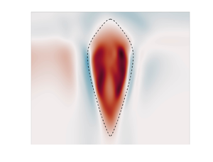
Examples of $\omega _{z,vortex}(x, y=0, z)$ for vortices from the $\mathrm {CV}\textit {--}\mathrm {Rot}$ and $\mathrm {CA}\unicode{x2013}\mathrm {Rot}$ families are shown in figure 5.

Figure 5.

Examples of $\omega _{z,vortex}(x,y=0,z)/(\,f\sin \theta _0)$ of two initial vortices in the $x$–$z$ plane at $y=0$. The horizontal axis is $x$, and the vertical axis is $z=z_c \sin \theta _0$. Both vortices have $H_{top}=50$ km, $H_{bot} =120$ km, $\omega _0 =3.0\times 10^{-5}$ s$^{-1}$, $\epsilon = 1.5$, $R_v =4600$ km and $L_r =2000$ km. (a) A constant-vorticity, area-varying $\mathrm {CV}\textit {--}\mathrm {Rot}$ vortex. (b) A constant-area, vorticity-varying $\mathrm {CA}\unicode{x2013}\mathrm {Rot}$ vortex. Note that the planetary vortices are pancake vortices. For example, our vertical domain size is $\sim$300 km, while the horizontal domain size is $\sim$100 000 km. The images are stretched along the vertical direction for graphical purposes. The vertical stretching applies to all figures of vertical slices presented.

For all four families of vortices, $z=z_0$ is the height of the $x$–$y$ plane where the initial anticyclones have their maximum values of $\tilde {P}_{vortex}/\bar {\rho }$ and $|\boldsymbol {v}_{vortex}|$. It is also the $x$–$y$ plane where the initial $\mathrm {CA}$ vortices have their maximum values of $|\tilde {\omega }_z|$, and the $x$–$y$ plane where the initial $\mathrm {CV}$ vortices have their maximum values of area. We define the mid-plane $z_{mid}(t)$ of the vortex as the height $z$ where the anticyclone has its maximum $\tilde {P}_{vortex}/\bar {\rho }$, and note that $z_{mid}(t)$ is a function of time, with $z_{mid}(t=0) = z_0$. Typically, the $x$–$y$ plane at $z_{mid}(t)$ is where a vortex in the $\mathrm {CA}$ family will have its biggest vertical vorticity, and where a vortex in the $\mathrm {CV}$ family will have its biggest horizontal area, so it is useful to track the flow fields in the mid-plane.

6.1. Orientation: aligned with the $z$ or $z_c$ axis?

The planetary vortices of interest in this study have low Rossby number ($Ro\lesssim 0.3$), and all the vortices that we examined have their final axes aligned approximately with the planet's spin axis ($z_c$ axis), even if they were initially aligned with the local gravity ($z$ axis). This is consistent with our previous findings (Zhang & Marcus Reference Zhang and Marcus2022). For example, figure 6 shows how the central axis of a vortex initially in the $\mathrm {CV}\textit {--}\mathrm {Rad}$ family changes from the beginning to the end of a simulation. For all heights $z$, we define the $y$ location of the vortex centre as

(6.1)\begin{equation} y_{ori}(z)=\frac{\iint[\tilde{P}_{vortex}(x,y,z)/\bar{\rho}(z)] \,y\,{\rm d}\kern0.06em x\,{\rm d}y}{\iint[\tilde{P}_{vortex}(x,y,z)/\bar{\rho}(z)] \, {\rm d}\kern0.06em x\,{\rm d}y}. \end{equation}

We use $\tilde {P}_{vortex}/\bar {\rho }$ as the weighting factor because it is almost never negative and is a good proxy for the stream function of the horizontal velocity. If ${\rm d}z/{\rm d}y_{ori} = \pm \infty$, then the central axis is aligned with the $z$ axis, and (using (2.11)) if ${\rm d}z/{\rm d}y_{ori} = \tan \theta _0$, then it is aligned with the $z_c$ axis. Initially, the vortex in figure 6 is aligned with the $z$ axis, but by the end of the simulation, for most values of $z$, the slope is ${\rm d}z/{\rm d}y_{ori} \simeq \tan \theta _0$, and the vortex is aligned with the $z_c$ axis. However, it must be noted that because the vertical thickness of the vortex is so much smaller than its diameter (${\sim }0.01$), the change in the location of the central axis during the simulation is extremely small.

Figure 6.

The change in the orientation of the central axis, $y_{ori}(z)$, of a vortex from initial condition to final state. The black dashed line has slope $\tan \theta _0$ and is parallel to the planet's spin, or $z_c$ axis. The blue vertical line shows the orientation of the initial vortex: $y_{ori} \equiv 0$ for all $z$, which is parallel to the direction of gravity or $z$ axis. The continuous orange curve shows $z$ as a function of $y_{ori}$ for the final vortex. Its central axis is aligned with the spin axis of the planet for almost all $z$, with the exception of the mid-plane near $z = -20$ km. The initial vortex is part of the $\mathrm {CV}\textit {--}\mathrm {Rad}$ family, is in near equilibrium, and is constructed using (5.15) with $H_{bot} = 120$ km, $H_{top} = 50$ km and $z_0 = 8.2$ km. For constructing $\omega _{z, vortex, 0}(x,y)$, we chose $Ro = -0.1$, or equivalently, $\epsilon = 1.5$.

The orange curve defining $y_{ori}(z)$ in figure 6 does not align perfectly with the $z_c$ axis. A small portion of $y_{ori}(z)$ (approximately $-20\ {\rm km} < z < 0\ {\rm km}$) is unaligned. Our simulations show that whether the central axis of a vortex aligns with the direction of the local gravity ($z$ axis) or with the $z_c$ axis depends on more than the value of the local Rossby number. However, we postpone that discussion for a future paper. All of our numerical simulations with initial vortices in the $\mathrm {CV}\textit {--}\mathrm {Rad}$ and $\mathrm {CA}\unicode{x2013}\mathrm {Rad}$ families ended with their central axes aligned approximately with the $z_c$ axis. For this reason, we confine the remainder of this section to the evolution of vortices that are initially in the $\mathrm {CV}\textit {--}\mathrm {Rot}$ and $\mathrm {CA}\unicode{x2013}\mathrm {Rot}$ families.

6.2. $\mathrm {CV}\textit {--}\mathrm {Rot}$

Using (5.18), the maximum vertical vorticity $\omega _{z,vortex}$ of the initial vortices is the same at each height, but the area of the vortex changes. We examined several initial $\mathrm {CV}\textit {--}\mathrm {Rot}$ vortices, and in all cases, the initial vortex converges to a large, quasi-steady vortex that drifts longitudinally. The vertical size of the vortex remains similar to its initial condition. An initially deeper $\mathrm {CV}\textit {--}\mathrm {Rot}$ vortex evolves to a deeper final state unless there is convectional instability locally (see § 8 for details).

To illustrate how this family of vortices evolves, § 6.2.1 shows an example of an initial vortex embedded in a constant-shear zonal velocity (case CV1). In § 6.2.2, we examine the same initial vortex embedded in the observed Jovian zonal velocity (case CV2). Both cases have $H_{bot} = 120$ km, $H_{top} = 50$ km, $\epsilon = 1.5$ (equivalently, $Ro = -0.1$) and $z_0 = 8.2$ km (equivalently, $700$ mbar; note that $z=0$, the top of the visible clouds, corresponds to $\bar {P} \simeq 1$ bar). One reason why we chose this value $z_0$ was so that there are no initial, local convective instabilities (see § 8).

6.2.1. Vortex embedded within a zonal velocity with constant shear (case CV1)

Figure 7 shows $\omega _{z,vortex}/|\,f\sin \theta _0|$ in the $x$–$y$ plane at the mid-plane at four different times. Because the initial condition is not in exact equilibrium, parts of it are torn apart by the zonal flow and roll up into small vortices. However, most of the initial vortex resists the zonal shear and remains intact. By the end of the simulation, all of the small vortices have merged back into the main vortex or become sheared out in the $x$ direction modifying the zonal flow, and there is only one large longitudinally drifting vortex. Figure 8 shows $\omega _{z,vortex}/|\,f\sin \theta _0|$ in the $x$–$z$ plane at $y=0$, which contains the central axis of the vortex. Throughout the simulation, the heights of the top and bottom of the vortex remain approximately constant. The hollowness, or local minimum, of $\omega _{z,vortex}$ at the central rotation axis of the vortex is visible at most values of $z$.

Figure 7.

Plots of $\omega _{z,vortex}(x,y)/|\,f\sin \theta _0|$ at the mid-plane of the vortex (case CV1). See supplementary movie 1 available at https://doi.org/10.1017/jfm.2024.132 for more details. At all times, the vortex mid-plane is defined as the height $z$ where the anticyclone has its maximum $\tilde {P}_{vortex}/\bar {\rho }$. The time is in units of Earth days: (a) $t=0$, (b) $t\sim 40$, (c) $t\sim 80$, (d) $t\sim 120$. The colour bar shows the value of $\omega _{z,vortex}(x,y)/|\,f\sin \theta _0|$. The turn-around time of this vortex is $\sim$4 days; that of the GRS is $\sim$6 days (Marcus Reference Marcus1993). In the first 40 days, the vortex remains mostly intact, but casts off many filaments that roll up into small vortices that are similar to those in the $\mathrm {CV}\textit {--}\mathrm {Rot}$ family. After 120 days, all of the small vortices have merged with the large vortex. The centre of the vortex is prominently hollow with a local minimum of $\omega _{z,vortex}$ at its centre. The vortex remains shielded, but most of the negative $\omega _{z,vortex}$ has moved to the vortex's northern and southern edges. We illustrate this case because it is qualitatively similar to all the simulations that we carried out with $\mathrm {CV}\textit {--}\mathrm {Rot}$ vortices embedded in constant zonal shear. There is little qualitative change of the vortex after 120 days.

Figure 8.

Plots of $\omega _{z,vortex}(x,y=0,z)/|\,f\sin \theta _0|$ in the $x$–$z$ plane of the vortex (case CV1). See supplementary movie 2 available at https://doi.org/10.1017/jfm.2024.132 for more details. The colour bar is as in figure 7. In this plane at day 40, the shed filaments have mostly negative values of $\omega _z$, and the hollowness along the central axis of the vortex has developed and extends from near the top of the vortex to near the bottom of the vortex. At day 120, some of the negative $\omega _z$ in the initial shield from other $x$–$z$ planes has become concentrated in this plane at $y=0$, and fills much of the east–west domain. Here, (a) $t = 0$ days, (b) $t \sim 40$ days, (c) $t \sim 80$ days, (d) $t \sim 120$ days.

The truly surprising result is that the vortex becomes hollow. The initial $\omega _{z,vortex}$ in figures 7(a) and 8(a) is non-hollow, but in the centre and along the central spin axis of the vortices in figures 7(b–d) and 8(b–d), $\omega _{z,vortex}$ is smaller than it is in the outer parts of the vortices. In our previous two-dimensional, quasi-geostrophic studies of vortex dynamics, we never found an initially non-hollow vortex spontaneously becoming hollow. Moreover, the only way that we found to prevent an initially hollow vortex from becoming non-hollow was by adding an artificial ‘bottom topography’ to the governing quasi-geostrophic equation of motion (Youssef Reference Youssef2000; Shetty et al. Reference Shetty, Asay-Davis and Marcus2006). However, Barranco & Marcus (Reference Barranco and Marcus2005) found stable hollow vortices in three-dimensional protoplanetary disk simulations, which indicates that the hollow vortex structure is indeed a three-dimensional effect.

Figure 9 shows $\tilde {\varTheta }_{vortex}/\bar {\varTheta }$ in the $x$–$z$ plane passing through the centre of the vortex. The cool top and warm bottom of the vortex occur because the major force balance in the $z$ component of the momentum equation is hydrostatic balance:

(6.2)\begin{equation} \frac{\partial }{\partial z}\biggl(\frac{\tilde{P}_{vortex}}{\bar{\rho}}\biggr)\sim \frac{\tilde{\varTheta}_{vortex}}{\bar{\varTheta}}\,g. \end{equation}

Figure 9.

Plots of $\tilde {\varTheta }_{vortex}(x,y=0,z)/\bar {\varTheta }$ (with values as shown in the colour bar) in the $x$–$z$ plane passing through the central axis of the vortex (case CV1). The mid-plane of the vortex lies in the horizontal band of white where $\tilde {\varTheta }_{vortex}(x,y,z) \simeq 0$. The high-$\tilde {\varTheta }_{vortex}$ annular ring at the edge of the vortex can be seen in (b–d) by noting that the white horizontal band has high ‘shoulders’ at the two edges of the vortex. The shoulders indicate that they contain higher $\tilde {\varTheta }_{vortex}/\bar {\varTheta }$ than the surrounding fluid at the same $z$. The shoulders are not present in (a) at $t=0$. The top of the vortex in (d) is at $z=60$ km, which corresponds to atmospheric pressure $35$ mbar. The tops of the large Jovian vortices are thought to be at a height above 140 mbar (Fletcher et al. Reference Fletcher2010) or heights above $z=37$ km in this figure. Here, (a) $t = 0$ days, (b) $t \sim 40$ days, (c) $t \sim 80$ days, (d) $t \sim 120$ days.

An anticyclone has a high pressure centre, so $\tilde {\varTheta }_{vortex}<0$ at heights above the mid-plane, and $\tilde {\varTheta }_{vortex}>0$ below the mid-plane to maintain the balance. The cooler temperature of the top of the GRS and other Jovian anticyclones has been observed many times (Flasar et al. Reference Flasar, Conrath, Pirraglia, Clark, French and Gierasch1981; Fletcher et al. Reference Fletcher2010, Reference Fletcher, Greathouse, Orton, Sinclair, Giles, Irwin and Encrenaz2016).

Figure 10 shows $\tilde {\varTheta }_{vortex}(x,y)/\bar {\varTheta }$ in the mid-plane of the vortex, corresponding to the horizontal white region in the middle of figure 9. It is not known whether the mid-planes of the Jovian vortices are at, below or above the visible cloud-top level at $z=0$ (i.e. at $\sim$1 bar). Initially, the mid-planes of our vortices are at $z_0$, and although the height of the mid-planes changes in time, they remain near $z_0$. Figure 10 shows a thin annulus of high $\tilde {\varTheta }_{vortex}/\bar {\varTheta }$ at the outer edge of the vortex, approximately coincident with the shield of negative $\omega _z$. This is an unexpected result, and the figure shows that this annulus was not present in the initial conditions. Because there is no corresponding anomaly in $\tilde {P}_{vortex}/\bar {P}$ at the location of this annulus (and because $\tilde {T}_{vortex}/\bar {T}=\tilde {\varTheta }_{vortex}/\bar {\varTheta }+(R/C_p) \tilde {P}_{vortex}/\bar {P}$), there is a high-temperature annulus of $\tilde {T}_{vortex}/\bar {T}$ at the outer edge of the vortex where the characteristic temperature of the annulus is approximately 1 K warmer than the surrounding fluid. Because this annulus was not present initially, and because $N^2 > 0$, the energy equation (2.22) shows that the annulus of high $\tilde {\varTheta }_{vortex}$ was created by a downward vertical velocity that formed in the annulus. That is, the high-temperature annulus was created by adiabatic heating. de Pater et al. (Reference de Pater, Wong, Marcus, Luszcz-Cook, Ádámkovics, Conrad, Asay-Davis and Go2010) observed $5\ \mathrm {\mu }{\rm m}$ bright annular rings around the GRS and other Jovian anticyclones, and hypothesized: (1) that the bright rings were created by down-welling velocities in the annuli that could not be observed directly; (2) that the adiabatic heating caused by the unseen down-welling locally dried out the atmosphere, making the annular regions free of clouds; and (3) that the $5\ \mathrm {\mu }{\rm m}$ radiation from the underlying, high-temperature atmosphere, which would normally be blocked by the clouds, would be observed. Figure 10 supports these hypotheses.

Figure 10.

Plots of $\tilde {\varTheta }_{vortex}(x,y)/\bar {\varTheta }$ on the mid-plane of the vortex (case CV1). This plane corresponds the white horizontal band in the middle of the vortex in figure 9. The characteristic difference between the temperature in the high-$\tilde {\varTheta }_{vortex}$ annular ring at the outer edge of the vortex and the ambient flow is approximately 1 K. The high-$\tilde {\varTheta }_{vortex}$ annulus in (b–d) is not present in (a) at $t=0$. The high-$\tilde {\varTheta }_{vortex}$ annular ring at the edge of the vortex corresponds to the high ‘shoulders’ in figures 9(b–d). Here, (a) $t = 0$ days, (b) $t \sim 40$ days, (c) $t \sim 80$ days, (d) $t \sim 120$ days.

Figure 11 shows the maximum values of $|\boldsymbol {v}_{vortex}|$, $\omega _{z,vortex}$, $\tilde {P}_{vortex}/\bar {\rho }$ and $v_{z,vortex}$ in each $x$–$y$ plane as functions of $z$ for the quasi-steady final vortex at day 120. The figure also shows $(\bar {N}^2 - N^2)$ as a function of $z$ along the central axis of the vortex. Figures 11(a,c) show that the vertical profiles of $|\boldsymbol {v}_{vortex}|$ and $\tilde {P}_{vortex}/\bar {\rho }$ are similar, as would be expected from geostrophic balance in (2.21). The mid-plane of the final vortex at 120 days is not very different from its initial location at $z=0$. Figure 11(b) shows that the vertical vorticity does not have a sharp maximum at the vortex mid-plane, but is nearly constant from $z=0$ down to $z= -100$ km. This is evidence that the final vortex is a $\mathrm {CV}\textit {--}\mathrm {Rot}$ vortex. Figure 11(d) shows that $v_z$ is $0.2\,\%$ of the full velocity at most in the three-dimensional simulation. Figure 11(e) shows $\bar {N}^2 - N^2 = - (g/\bar {\varTheta })(\partial \tilde {\varTheta }/\partial z)$, which is the stratification due to the net velocity (zonal flow plus vortex) along the central axis of the vortex. The value is non-dimensionalized by $(\,f\sin \theta _0)^2$. When this quantity is greater than zero, it means that the vortex has locally mixed the fluid in a way to de-stratify the vortex; the mixing has increased the potential temperature at the bottom of the vortex at the expense of the potential temperature at the top of the vortex. (In other words, mixing has increased the potential mass density at the top of the vortex at the expense of the mass density at the bottom of the vortex, making it more prone to local convective instabilities.) In regions where $\tilde {N}^2_{vortex}/g < 0$, mixing has super-stratified the fluid, making it more stable to convection.

Figure 11.

Vertical profiles of the vortex in case CV1. (a) Maximum $|\boldsymbol {v}_{vortex}|$ at each $x$–$y$ plane as a function of $z$. (b) Maximum $\omega _{z,vortex}$ at each $x$–$y$ plane as a function of $z$. (c) Maximum $\tilde {P}_{vortex}/\bar {\rho }$ at each $x$–$y$ plane as a function of $z$. (d) Maximum $|{v}_{z,vortex}|$ at each $x$–$y$ plane as a function of $z$: $\|\boldsymbol {v}_{z,vortex}\|_{\infty }/\|\boldsymbol {v}_{\perp,vortex}\|_{\infty }\times 100$. (e) Plot of $(\bar {N}^2-N^2)/(\,f\sin \theta _0)^2$ along the $z$ axis of the vortex. Plots (a–c) are normalized by their maximum values; (d) is normalized by the maximum $|\boldsymbol {v}_{vortex}|$ of the vortex. The green dashed line in (e) indicates where $\bar {N}^2-N^{2} =0$. Plot (e) shows that near the mid-plane, the vortex is de-stratified, making it more prone to convective instabilities; whereas at the vortex's top and bottom, the fluid is superstratified and more resistant to convection. Note that the mid-plane location is $z=0.58$ km ($975$ mbar) at day 120, slightly lower than the height of its initial location at $z_0=8.2$ km ($700$ mbar). See text for details.

6.2.2. Vortex embedded in the Jovian zonal velocity (case CV2)

Note that case CV1 is conducted in a constant-shear zonal flow without the locations of maximum and minimum zonal velocity. On the other hand, Shetty et al. (Reference Shetty, Asay-Davis and Marcus2007) suggested that the latter is important to make hollow vortices in stable equilibrium in a quasi-geostrophic system with bottom topography. We repeated the numerical calculation with the same initial vortex that we used in the CV1 case, but embedded in the Jovian zonal velocity (blue curve in figure 3), rather than with the straight orange line (which has no local maximum or minimum velocities). The purpose of this simulation is to see if including the locations of maximum and minimum zonal velocity can significantly affect the simulation result. Figures 12–14 show the vertical vorticity and potential temperature of this new vortex labelled CV2. To our surprise, the two final vortices are qualitatively similar, other than the fact that the horizontal area of $\omega _z$ of the vortex is smaller than that of the CV1 vortex at day 120. They are both shielded and both developed warm, thin annular rings at their outer edges like the large Jovian anticyclones. In addition, they both developed hollow interiors like the GRS. Our result indicates that the locations (or existence) of the maximum and minimum zonal velocities are not important for the vortex features that we capture in both simulations (hollowness, warm ring, etc.).

Figure 12.

Plots of $\omega _{z,vortex}(x,y)/|\,f\sin \theta _0|$ of the CV2 vortex plotted as we did for the CV1 vortex in figure 7. The two horizontal arrows at the right-hand side indicate the latitudes where the zonal flow in figure 3 has local maximum and minimum values. The arrows point in the direction of the local zonal flow. Here, (a) $t = 0$ days, (b) $t \sim 40$ days, (c) $t \sim 80$ days, (d) $t \sim 120$ days.

Figure 13.

Plots of $\omega _{z,vortex}(x,y=0,z)/|\,f\sin \theta _0|$ of the CV2 vortex plotted as we did for the CV1 vortex in figure 8. Here, (a) $t = 0$ days, (b) $t \sim 40$ days, (c) $t \sim 80$ days, (d) $t \sim 120$ days.

Figure 14.

Plots of $\tilde {\varTheta }(x,y)/\bar {\varTheta }$ of the CV2 vortex plotted as we did for the CV1 vortex in figure 9. The black arrows indicates the locations of the westward/eastward zonal flow's maximum location. Here, (a) $t = 0$ days, (b) $t \sim 40$ days, (c) $t \sim 80$ days, (d) $t \sim 120$ days.

Although we did not intend to recover the velocity and temperature field of any specific Jovian vortex in this study, the velocities of the CV1 and CV2 quasi-steady vortices are qualitatively similar to the GRS because of their hollow interiors. This can be seen in figure 15, which shows the $\omega _{z,vortex}$ of the GRS and of the CV2 vortex along their north–south minor principal axes as functions of $y$, at the cloud-top plane. The interiors of the vortices are the regions in $y$ where $\omega _{z,vortex} >0$; the shields are the regions just outside interiors where $\omega _{z,vortex} <0$. The $\omega _{z,vortex}$ of a non-hollow shielded vortex would decrease monotonically as a function of $|y|$ from its maximum value at the latitude of the vortex centre at $y=0$ until it became negative in the shield, and then it would increase to zero at the outer edge of the shield. Both the GRS and CV2 have pronounced local minima of $\omega _{z,vortex}$ at $y=0$ surrounded in the north and south by large ‘shoulders’ of positive $\omega _{z,vortex}$. A measure of the hollowness of a vortex is the ratio of the largest value of $\omega _{z,vortex}$ in the shoulders divided by the local minimum value of $\omega _{z,vortex}$ at the vortex centre. Both the GRS and CV2 have similar ratios, $\sim$2. However, the GRS is larger than CV2, and its region of hollowness is also larger.

Figure 15.

Comparison of the $\omega _{z,vortex}$ of the CV2 vortex at the cloud-top plane and the observed GRS along the principle, minor, north–south or $y$ axis: (a) CV2, (b) the observed GRS profile from Wong et al. (Reference Wong, Marcus, Simon, de Pater, Tollefson and Asay-Davis2021). The black arrows indicate the locations of the extrema of westward/eastward zonal velocity. The hollowness ratio (defined as the maximum value of $\omega _{z,vortex}$ in the ‘shoulders’ divided by its local minimum value at the vortex centre – see text for details) of the GRS and CV2 are both $\sim$2. The main difference between the GRS and CV2 is that the GRS is larger.

6.3. $\mathrm {CA}\unicode{x2013}\mathrm {Rot}$

Using (5.14) to create an initial $\mathrm {CA}\unicode{x2013}\mathrm {Rot}$ vortex makes the horizontal area of the vertical vorticity $\omega _{z,vortex}$ of the initial vortex the same at each height, but the magnitude of $\omega _{z,vortex}$ decreases away from the mid-plane, vanishing at the tops and bottoms of the vortex. None of our simulations that began with $\mathrm {CA}\unicode{x2013}\mathrm {Rot}$ vortices produced a quasi-steady $\mathrm {CA}\unicode{x2013}\mathrm {Rot}$ vortex at the end of the simulation. The initial vortex either quickly filamented into smaller vortices due to the shear of the zonal flow being much greater than $\omega _{z,vortex}$ at the tops and bottoms of the vortices, or broke apart due to a local convective instability (as discussed in § 8 because the top of the initial vortex is too close to the mid-plane). In all cases, we found that the flow creates one or more quasi-steady $\mathrm {CV}\textit {--}\mathrm {Rot}$ vortices at the end of the simulation. This is shown in figures 16 and 17 for a vortex embedded in a zonal flow with constant shear (case CA1), and in figures 18 and 19 for a vortex embedded in the Jovian zonal flow shown in figure 3 (case CA2). For both cases, $H_{top} = 120$ km, $H_{bot} = 50$ km, $\epsilon = 1.5$ (equivalently, $Ro =-0.1$) and $z_0 = 8.2$ km (equivalently, $\bar {P}=700$ mbar). Initially, the $\mathrm {CA}\unicode{x2013}\mathrm {Rot}$ vortices are column-like in the $x$–$z$ plane, with the area of the vortex on each $x$–$y$ plane identical. For both cases, the initial vortices fragment within the first 40 days into filaments that roll up into smaller vortices. However, during that same time, the initial vortex and the smaller vortices that it spawns evolve into $\mathrm {CV}\textit {--}\mathrm {Rot}$ vortices. By day 80, many of the smaller vortices have merged with the large vortex, and by day 120, only a few vortices remain unmerged. We truncated the calculations after day 120 because the purpose of the calculations is to show that the $\mathrm {CA}\unicode{x2013}\mathrm {Rot}$ vortices are far from equilibrium and that they quickly evolve into $\mathrm {CV}\textit {--}\mathrm {Rot}$ vortices. Based on two-dimensional vortex dynamics in zonal flows, we expect that if we continue calculation, the vortices whose central latitudes are closer together than the semi-minor radius of the largest vortex will eventually merge together.

Figure 16.

Evolution of $\omega _{z,vortex}(x,y)/|\,f\sin \theta _0|$ in the mid-plane of an initial $\mathrm {CA}\unicode{x2013}\mathrm {Rot}$ vortex embedded in a constant zonal shear (case CA1). The surviving vortices are all part of the $\mathrm {CV}\textit {--}\mathrm {Rot}$ family (see figure 17). Here, (a) $t = 0$ days, (b) $t \sim 40$ days, (c) $t \sim 80$ days, (d) $t \sim 120$ days.

Figure 17.

Evolution of $\omega _{z,vortex}(x,y=0,z)/|\,f\sin \theta _0|$ of the CA1 vortex in figure 16 shown in the $x$–$z$ plane passing through the central axis of the initial vortex. See supplementary movie 3 available at https://doi.org/10.1017/jfm.2024.132 for more details. The horizontal area of the initial vortex in (a) is approximately constant in $z$, but the magnitude of $\omega _{z,vortex}$ decreases with distance from the mid-plane, making it part of the $\mathrm {CA}\unicode{x2013}\mathrm {Rot}$ family. By day 40, the initial vortex and the large vortices spawned from it have changed from $\mathrm {CA}\unicode{x2013}\mathrm {Rot}$ vortices to $\mathrm {CV}\textit {--}\mathrm {Rot}$ vortices. Here, (a) $t = 0$ days, (b) $t \sim 40$ days, (c) $t \sim 80$ days, (d) $t \sim 120$ days.

Figure 18.

Plots of $\omega _{z,vortex}(x,y)/|\,f\sin \theta _0|$ in the mid-plane of the same initial vortex shown in figure 16, but embedded in the Jovian zonal flow. We call this the CA2 vortex. At 120 days, there are two large $\mathrm {CV}\textit {--}\mathrm {Rot}$ vortices and one smaller one. Based on simulations of two-dimensional quasi-geostrophic vortices, we believe that the difference in the number of vortices that survive for 120 days in this figure and in figure 16 is not physically significant. The initial filamentation of the out-of-equilibrium initial vortices is sensitive to small details of the initial flow, and when the filaments roll up into vortices, their latitudes are also sensitive to the details of the initial condition. If many of the rolled-up vortices have latitudes far from the latitude of the surviving vortex, then few of them will merge together. Here, (a) $t = 0$ days, (b) $t \sim 40$ days, (c) $t \sim 80$ days, (d) $t \sim 120$ days.

Figure 19.

Plots of $\omega _{z,vortex}(x,y=0,z)/|\,f\sin \theta _0|$ in the $x$–$z$ plane passing through the central axis of the initial vortex (case CA2). Although the initial vortex in (a) is in the $\mathrm {CA}\unicode{x2013}\mathrm {Rot}$ family, the surviving vortices in (d) are in the $\mathrm {CV}\textit {--}\mathrm {Rot}$ family. Here, (a) $t = 0$ days, (b) $t \sim 40$ days, (c) $t \sim 80$ days, (d) $t \sim 120$ days.

6.4. How the energy equation comes to equilibrium

In § 5.1, we showed that our initial conditions of the vortices were such that they satisfy the continuity equation (2.20), all three components of the steady momentum equation (2.21), and the ideal gas equations (2.23) and (2.24). However, because $v_z \equiv 0$, none of our initial conditions satisfied the energy equation (2.22). Numerically, we found that with the exception of (2.22), the full equations of motion (2.20)–(2.24) were nearly satisfied because the initial characteristic times for ${\boldsymbol {v}}$, $\tilde {\rho }$ and $\tilde {P}$ to change were long compared to the turn-around time of the vortex, but the initial characteristic time for $\tilde {\varTheta }$ to change was much faster. Of the two terms on the far right-hand side of (2.22), only $({\boldsymbol {v}}_{\perp } \boldsymbol {\cdot } \boldsymbol {\nabla }_{\perp }) \tilde {\varTheta }$ can initially change $\partial \tilde {\varTheta }/\partial t$ because $v_z$ is initially zero. When the vortex reaches its final steady state, the magnitude of the $({\boldsymbol {v}}_{\perp } \boldsymbol {\cdot } \boldsymbol {\nabla }_{\perp }) \tilde {\varTheta }$ term has decreased approximately by a factor of 3 from its initial magnitude, and is balanced primarily by the $\bar {N}^2 v_z \bar {\varTheta }/g$ term. Thus even though $v_z$ is small compared to $v_{\perp }$ (see (7.1) below), $v_z$ cannot be zero and plays an essential role in creating the final steady vortex. (If $v_z=0$, then the only way that the steady version of (2.22) could be satisfied would be if the isocontours of $\tilde {\varTheta }$ coincide with the two-dimensional horizontal streamlines.)

7.1. Scaling analysis of the vertical vorticity equation

In § 5.2, we showed that a steady vortex with $v_z \equiv 0$ has $(\boldsymbol {v}_\perp \boldsymbol {\cdot }\boldsymbol {\nabla }_\perp )(\omega _z + \beta y) =0$. However, none of our computed vortices has $v_z \equiv 0$, and it is important to understand how small $(\boldsymbol {v}_\perp \boldsymbol {\cdot }\boldsymbol {\nabla }_\perp )(\omega _z + \beta y)$ is, how it scales with the small dimensionless parameters of the flow, such as the Rossby number $Ro \equiv \|\omega _z\|_{\infty }/(2 f |\sin \theta _0|)$, and what terms balance it in the vertical component of the anelastic vorticity (2.26). To understand how the various terms in (2.26) scale, we must first understand how $\langle v_z \rangle / \langle v_{\perp } \rangle$ scales, where angle brackets around a quantity are defined to mean the ‘characteristic value’ of that quantity. We also define the characteristic horizontal length of the vortex $L \equiv \|v_{\perp }\|_2/\|\omega _z\|_2$ evaluated at the vortex mid-plane. We also define the characteristic vertical size of a vortex $H \equiv \|v_{\perp }\|_2/\|\omega _{\perp }\|_2$ evaluated at the vortex mid-plane where the $L_2$ norms are taken over the horizontal area of the vortex. For the types of vortices considered here, which are not vertically confined by walls, the vertical and horizontal components of the velocity have the same vertical scale $H$, and horizontal scale $L$. In our calculations, we found that $H$ is the approximate vertical scale height of $\bar {\rho }$ and $\bar {P}$, smaller than the prescribed vertical depth $H_{top}$ or $H_{bot}$. Our result shows clearly that the vertical characteristic length scale of Jovian vortices can be different from their depth, which is similar to the findings that the Rossby deformation radius is less than the semi-minor radius of the GRS (Marcus Reference Marcus1988; Dowling & Ingersoll Reference Dowling and Ingersoll1989; Shetty & Marcus Reference Shetty and Marcus2010).

Note that these scaling relationships differ from those used for quasi-geostrophic homogeneous flows, where it is assumed that the vertical scale height of the horizontal component of the velocity is much greater than that of the vertical component (see Chapter 6 of Pedlosky Reference Pedlosky1982). Our numerical calculations suggest the following scalings:

(7.1)$$\begin{gather} \langle v_z \rangle = Ro^2\,\frac{{H}}{L}\,\langle v_{{\perp}} \rangle, \end{gather}$$

(7.2)$$\begin{gather}\left\langle (\boldsymbol{\nabla}_\perp\boldsymbol{\cdot}\boldsymbol{v}_\perp) \right\rangle = \langle v_z \rangle/H = Ro^2 \, \langle v_{{\perp}} \rangle/L, \end{gather}$$

(7.3)$$\begin{gather}\left\langle (\boldsymbol{\nabla} \boldsymbol{\cdot}\boldsymbol{v}) \right\rangle = \langle v_z \rangle/H = Ro^2\,\langle v_{{\perp}} \rangle/L, \end{gather}$$

(7.4)$$\begin{gather}\left\langle (\boldsymbol{v}_\perp\boldsymbol{\cdot} \boldsymbol{\nabla}_\perp)(\omega_z + \beta y)\right\rangle = Ro \left[{\frac{\langle v_\perp \rangle}{L}}\right]^2, \end{gather}$$

(7.5)$$\begin{gather}\left\langle\, f \, \sin\theta_0+ \beta y) (\boldsymbol{\nabla}_\perp\boldsymbol{\cdot}\boldsymbol{v}_\perp) \right\rangle = Ro \left[{\frac{\langle v_\perp \rangle}{L}}\right]^2, \end{gather}$$

(7.6)$$\begin{gather}\left\langle \omega_z (\boldsymbol{\nabla}_\perp\boldsymbol{\cdot}\boldsymbol{v}_\perp) \right\rangle = Ro^2 \left[{\frac{\langle v_\perp \rangle}{L}}\right]^2, \end{gather}$$

(7.7)$$\begin{gather}\left\langle v_z\,\frac{\partial \omega_z}{\partial z}\right\rangle = Ro^2 \left[{\frac{\langle v_\perp \rangle}{L}}\right]^2, \end{gather}$$

(7.8)$$\begin{gather}\left\langle ({\boldsymbol{\omega}}_\perp\boldsymbol{\cdot}\boldsymbol{\nabla}_\perp)v_z\right\rangle = Ro^2 \left[{\frac{\langle v_\perp \rangle}{L}}\right]^2, \end{gather}$$

(7.9)$$\begin{gather}\left\langle (\,f \cos_0 - \beta y \tan \theta_0)\,\frac{\partial v_z}{\partial y}\right\rangle = Ro\cot \theta_0\, {\frac{H}{L}} \left[{\frac{\langle v_\perp \rangle}{L}}\right]^2, \end{gather}$$

(7.10)$$\begin{gather}\left\langle \beta v_z \tan \theta_0 \right\rangle = Ro\,{\frac{H}{r_0}} \left[{\frac{\langle v_\perp \rangle}{L}}\right]^2. \end{gather}$$

Note that the scaling equations (7.4)–(7.10) are for the seven terms on the right-hand side of (2.26). This tells us that when the flow is steady, although $(\boldsymbol {v}_\perp \boldsymbol {\cdot }\boldsymbol {\nabla }_\perp )(\omega _z + \beta y)$ is not identically zero as in (5.2), it is small compared to $[{{\langle v_\perp \rangle }/{L}}]^2$. Thus the two-dimensional streamlines and the isocontours of $(\omega _z + \beta y)$ are nearly coincident, as argued in § 5.2. We remind the reader that this needed coincidence was the basis on which we argued that the CA family of vortices was far from equilibrium, whereas the CV family was near equilibrium. Scaling equations (7.4)–(7.10) also tell us that the dominant balance in (2.26) is between $(\boldsymbol {v}_\perp \boldsymbol {\cdot }\boldsymbol {\nabla }_\perp )(\omega _z + \beta y)$ and $f \sin \theta _0\, (\boldsymbol {\nabla }_\perp \boldsymbol {\cdot }\boldsymbol {v}_\perp )$. This balance is illustrated in figure 20, which shows the values of $-(\boldsymbol {v}_\perp \boldsymbol {\cdot }\boldsymbol {\nabla }_\perp )(\omega _z + \beta y)$ (figure 20a) and $-f \sin \theta \,(\boldsymbol {\nabla }_\perp \boldsymbol {\cdot }\boldsymbol {v}_\perp )$ (figure 20b) in the mid-plane. These two terms do not exactly cancel each other near the centre because they both become small there (due to the hollowness of the vortex), and the other terms in (2.26) become comparable to them. Note that for most Jovian vortices and our numerical simulations here, $Ro\sim 0.1$. For the simulations presented here, $H/L\sim 0.01$. The value of $H/L$ for Jovian vortices is not well constrained by observations. Also note that $\langle L \rangle /r_0 \simeq 0.03$ for the largest Jovian vortices.

Figure 20.

The dominant two components of (2.26) at the vortex mid-plane (using the final state of case CV1). The plotted values are normalized by ${\|\boldsymbol {v}\|_\infty ^2}/{L^2}$: (a) $-(\boldsymbol {v}_\perp \boldsymbol {\cdot }\boldsymbol {\nabla }_\perp ) \omega _z$, (b) $-f \sin \theta _0\,(\boldsymbol {\nabla }_\perp \boldsymbol {\cdot }\boldsymbol {v}_\perp )$.

7.2. Shape of the vortex

The shapes of $\omega _{z,vortex}$ of the steady vortices in the $x$–$z$ plane all have a distinctive ‘ice cream cone’ shape (e.g. figures 8(d), 13(d), 17(d) and 19(d)). We can explain these by recalling that

(7.11)\begin{equation} N^2\equiv\frac{g}{\bar{\varTheta}}\,\frac{\partial \varTheta}{\partial z}=\bar{N}^2+\frac{g}{\bar{\varTheta}}\,\frac{\partial \tilde{\varTheta}}{\partial z}, \end{equation}

and using the hydrostatic approximation (6.2),

(7.12)\begin{align} N^2&=\bar{N}^2+\frac{g}{\bar{\varTheta}}\,\frac{\partial }{\partial z}\biggl[\frac{\bar{\varTheta}}{g}\,\frac{\partial }{\partial z}\biggl(\frac{\tilde{P}}{\bar{\rho}}\biggr)\biggr] \end{align}

(7.13)\begin{align} &=\bar{N}^2+\frac{\mathrm{d} \ln\bar{\varTheta}}{\mathrm{d} z}\,\frac{\partial }{\partial z}\biggl(\frac{\tilde{P}}{\bar{\rho}}\biggr)+\frac{\partial^2}{\partial z^2}\biggl(\frac{\tilde{P}}{\bar{\rho}}\biggr)\!. \end{align}

To eliminate $({\tilde {P}}/{\bar {\rho }})$ in (7.13), we use the small-Rossby number limit (quasi-geostrophic approximation) of (5.3) with $\beta =0$:

(7.14)\begin{equation} (\,f \sin \theta_0)\,\omega_z(x, y, z) = \nabla_\perp^2 \biggl(\frac{\tilde{P}(x, y, z)}{\bar{\rho}}\biggr)\!. \end{equation}

For each $z$ within the vortex, averaging (7.14) over the horizontal area within the vortex, we define ${\mathcal {A}}(z)$ with

(7.15) \begin{equation} (\,f \sin \theta_0)\,\omega_z(z)\biggl|_{averaged} = \biggl[\nabla_\perp^2 \biggl(\frac{\tilde{P}}{\bar{\rho}}\biggr)\biggr]\biggl|_{averaged} \equiv- \biggr[\biggl(\frac{\tilde{P}}{\bar{\rho}}\biggr)\biggl|_{averaged}\biggr] \biggl/ {\mathcal{A}}(z), \end{equation}

where ${\mathcal {A}}(z)$ has dimensions of length squared. Our numerical calculations show that $\sqrt {{\mathcal {A}}(z)}$ is approximately equal to the mean cross-sectional radius of the vortex. (We first found this relationship empirically in Boussinesq vortices; Hassanzadeh et al. Reference Hassanzadeh, Marcus and Le Gal2012.) Because all the final, statistically steady vortices computed here, regardless of their initial conditions, are $\mathrm {CV}\textit {--}\mathrm {Rot}$ vortices, it is reasonable to approximate $\omega _z(z)|_{averaged}$ as independent of $z$, and assign it a value $\omega _A$. Thus (7.13)–(7.15) become

(7.16)\begin{equation} \frac{{\rm d}^2{\mathcal{A}}}{{\rm d}z^2}+\frac{\mathrm{d} \ln\bar{\varTheta}}{\mathrm{d} z}\,\frac{\mathrm{d} {\mathcal{A}}}{\mathrm{d} z}=-\frac{N^2(z)|_{averaged}-\bar{N}^2(z)}{f \omega_A \sin \theta_0 }. \end{equation}

Given ${\rm d}\ln \bar {\varTheta }/{\rm d}z$, $\bar {N}^2(z)$, $N(z)|_{averaged}$ and $\omega _A$, we can solve (7.16) for $\sqrt {{\mathcal {A}}(z)}$, the mean radius of the vortex, using the boundary conditions that ${\mathcal {A}} =0$ at the top and bottom of the vortex. Figure 21 shows the results of solving (7.16) for $\sqrt {{\mathcal {A}}(z)}$ for the CV1 and CV2 vortices, and that the equation works well in describing the vortex shapes.

Figure 21.

Comparing $2\sqrt {{\mathcal {A}}(z)}$ (dashed line) to the vertical vorticity $\omega _{z,vortex}(x,y=0,z)/|\,f\sin \theta _0|$ of the (a) CV1 and (b) CV2 vortices in the $x$–$z$ plane going through the centre of each vortex. The factor of 2 is to make the boundary close to the visual boundary of the vortex.