2 Theory

Electrostatic units are utilized, the temperatures are provided in energy units. The following notations are employed; $\unicode[STIX]{x1D6FC}=\{e,i\}$ for the plasma species, $e$ for the elementary charge, $(q_{\unicode[STIX]{x1D6FC}},m_{\unicode[STIX]{x1D6FC}},n_{\unicode[STIX]{x1D6FC}},T_{\unicode[STIX]{x1D6FC}})$ for the charge, mass, number density and temperature, $v_{\text{T}\unicode[STIX]{x1D6FC}}=\sqrt{T_{\unicode[STIX]{x1D6FC}}/m_{\unicode[STIX]{x1D6FC}}}$ for the thermal velocities, $\unicode[STIX]{x1D714}_{\text{p}\unicode[STIX]{x1D6FC}}=\sqrt{(4\unicode[STIX]{x03C0}q_{\unicode[STIX]{x1D6FC}}^{2}n_{\unicode[STIX]{x1D6FC}})/m_{\unicode[STIX]{x1D6FC}}}$ for the species plasma frequencies, $\unicode[STIX]{x1D706}_{\text{D}\unicode[STIX]{x1D6FC}}=\sqrt{T_{\unicode[STIX]{x1D6FC}}/(4\unicode[STIX]{x03C0}q_{\unicode[STIX]{x1D6FC}}^{2}n_{\unicode[STIX]{x1D6FC}})}$ for the species Debye lengths and $\unicode[STIX]{x1D706}_{\text{D}}$ for the plasma Debye length defined by $1/\unicode[STIX]{x1D706}_{\text{D}}^{2}=1/\unicode[STIX]{x1D706}_{\text{De}}^{2}+1/\unicode[STIX]{x1D706}_{\text{Di}}^{2}$ .

In homogeneous weakly coupled plasmas, plasma density fluctuations are fully described by the two-point space–time correlation function defined by $C_{\boldsymbol{r},\boldsymbol{r}^{\prime },t,t^{\prime }}^{\unicode[STIX]{x1D6FC}}=\langle \unicode[STIX]{x1D6FF}n_{\boldsymbol{ r},t}^{\unicode[STIX]{x1D6FC}}\unicode[STIX]{x1D6FF}n_{\boldsymbol{ r}^{\prime },t^{\prime }}^{\unicode[STIX]{x1D6FC}}\rangle$ , where the brackets $\langle \cdots \rangle$ denote the ensemble average over the different realizations of the system, which reduces to $C_{\boldsymbol{r},t}^{\unicode[STIX]{x1D6FC}}=\langle \unicode[STIX]{x1D6FF}n_{\boldsymbol{r},t}^{\unicode[STIX]{x1D6FC}}\unicode[STIX]{x1D6FF}n_{\mathbf{0},0}^{\unicode[STIX]{x1D6FC}}\rangle$ due to the spatio-temporal translation symmetry (Klimontovich Reference Klimontovich1967; Akhiezer et al. Reference Akhiezer, Akhiezer, Polovin, Sitenko and Stepanov1975; Alexandrov et al. Reference Alexandrov, Bogdankevich and Rukhadze1984). Unless the heuristic non-interacting limit is considered (Akhiezer et al. Reference Akhiezer, Akhiezer, Polovin, Sitenko and Stepanov1975; Alexandrov et al. Reference Alexandrov, Bogdankevich and Rukhadze1984; Tolias et al. Reference Tolias, Ratynskaia, Panarese, Longo and de Angelis2015), there are no analytic expressions for $C_{\boldsymbol{r},t}^{\unicode[STIX]{x1D6FC}}$ . However, convenient closed form relations exist for its space–time Fourier transform $S_{\boldsymbol{k},\unicode[STIX]{x1D714}}^{\unicode[STIX]{x1D6FC}}=\langle |\unicode[STIX]{x1D6FF}n_{\boldsymbol{k},\unicode[STIX]{x1D714}}^{\unicode[STIX]{x1D6FC}}|^{2}\rangle$ , typically coined as the spectral density of the plasma density fluctuations. For collisionless non-relativistic fully ionized multi-component plasmas in the absence of external electromagnetic fields, the spectral density of the electron density fluctuations has the general form (Sheffield Reference Sheffield1975)

(2.1) $$\begin{eqnarray}S_{\boldsymbol{k},\unicode[STIX]{x1D714}}^{\text{e}}=\left|1-\frac{\unicode[STIX]{x1D712}_{\boldsymbol{k},\unicode[STIX]{x1D714}}^{\text{e}}}{\unicode[STIX]{x1D716}_{\boldsymbol{k},\unicode[STIX]{x1D714}}}\right|^{2}S_{\boldsymbol{ k},\unicode[STIX]{x1D714}}^{\text{e},(0)}+\left|\frac{\unicode[STIX]{x1D712}_{\boldsymbol{k},\unicode[STIX]{x1D714}}^{\text{e}}}{\unicode[STIX]{x1D716}_{\boldsymbol{k},\unicode[STIX]{x1D714}}}\right|^{2}\mathop{\sum }_{\unicode[STIX]{x1D6FC}\neq \text{e}}\frac{q_{\unicode[STIX]{x1D6FC}}^{2}}{e^{2}}S_{\boldsymbol{k},\unicode[STIX]{x1D714}}^{\unicode[STIX]{x1D6FC},(0)},\end{eqnarray}$$

where $\unicode[STIX]{x1D716}_{\boldsymbol{k},\unicode[STIX]{x1D714}}=1+\sum _{\unicode[STIX]{x1D6FC}}\unicode[STIX]{x1D712}_{\boldsymbol{k},\unicode[STIX]{x1D714}}^{\unicode[STIX]{x1D6FC}}$ is the plasma dielectric permittivity, $\unicode[STIX]{x1D712}_{\boldsymbol{k},\unicode[STIX]{x1D714}}^{\unicode[STIX]{x1D6FC}}$ are the plasma species susceptibilities and $S_{\boldsymbol{k},\unicode[STIX]{x1D714}}^{\unicode[STIX]{x1D6FC},(0)}$ are the spectral densities of the natural plasma density fluctuations. The latter two quantities are given by

(2.2) $$\begin{eqnarray}\displaystyle \unicode[STIX]{x1D712}_{\boldsymbol{k},\unicode[STIX]{x1D714}}^{\unicode[STIX]{x1D6FC}} & = & \displaystyle \frac{4\unicode[STIX]{x03C0}q_{\unicode[STIX]{x1D6FC}}^{2}}{m_{\unicode[STIX]{x1D6FC}}k^{2}}\int \frac{1}{\unicode[STIX]{x1D714}-\boldsymbol{k}\boldsymbol{\cdot }\boldsymbol{v}+\imath 0}\left[\boldsymbol{k}\boldsymbol{\cdot }\frac{\unicode[STIX]{x2202}\unicode[STIX]{x1D6F7}_{\unicode[STIX]{x1D6FC}}(\boldsymbol{v})}{\unicode[STIX]{x2202}\boldsymbol{v}}\right]\,\text{d}^{3}v\nonumber\\ \displaystyle & = & \displaystyle \frac{1}{k^{2}\unicode[STIX]{x1D706}_{\text{D}\unicode[STIX]{x1D6FC}}^{2}}\left[1+\unicode[STIX]{x1D701}_{\unicode[STIX]{x1D6FC}}\text{e}^{-\unicode[STIX]{x1D701}_{\unicode[STIX]{x1D6FC}}^{2}}\left(\imath \sqrt{\unicode[STIX]{x03C0}}-2\int _{0}^{\unicode[STIX]{x1D701}_{\unicode[STIX]{x1D6FC}}}\text{e}^{t^{2}}\,\text{d}t\right)\right],\end{eqnarray}$$

(2.3) $$\begin{eqnarray}\displaystyle S_{\boldsymbol{k},\unicode[STIX]{x1D714}}^{\unicode[STIX]{x1D6FC},(0)} & = & \displaystyle \frac{1}{(2\unicode[STIX]{x03C0})^{3}}\int \unicode[STIX]{x1D6FF}(\unicode[STIX]{x1D714}-\boldsymbol{k}\boldsymbol{\cdot }\boldsymbol{v})\unicode[STIX]{x1D6F7}_{\unicode[STIX]{x1D6FC}}(\boldsymbol{v})\,\text{d}^{3}v=\frac{1}{(2\unicode[STIX]{x03C0})^{7/2}}\frac{n_{\unicode[STIX]{x1D6FC}}}{kv_{\text{T}\unicode[STIX]{x1D6FC}}}\text{e}^{-\unicode[STIX]{x1D701}_{\unicode[STIX]{x1D6FC}}^{2}},\end{eqnarray}$$

with $\unicode[STIX]{x1D701}_{\unicode[STIX]{x1D6FC}}=\unicode[STIX]{x1D714}/(\sqrt{2}kv_{\text{T}\unicode[STIX]{x1D6FC}})$ . The first equality is valid for an arbitrary distribution function, whereas the second equality is valid for a Maxwellian distribution function $\unicode[STIX]{x1D6F7}_{\unicode[STIX]{x1D6FC}}(\boldsymbol{v})=n_{\unicode[STIX]{x1D6FC}}[m_{\unicode[STIX]{x1D6FC}}/(2\unicode[STIX]{x03C0}T_{\unicode[STIX]{x1D6FC}})]^{3/2}\exp [-m_{\unicode[STIX]{x1D6FC}}v^{2}/(2T_{\unicode[STIX]{x1D6FC}})]$ . It is apparent from (2.1) that $S_{\boldsymbol{k},\unicode[STIX]{x1D714}}^{\text{e}}$ will have maxima at $\unicode[STIX]{x1D716}_{\boldsymbol{k},\unicode[STIX]{x1D714}}\simeq 0$ , which correspond to the weakly damped eigenmodes of the system.

Let us consider a thermal plasma consisting of electrons and a singly positively charged ion species; $n_{\text{e}}=n_{\text{i}}=n$ , $T_{\text{e}}=T_{\text{i}}=T$ and $m_{\text{i}}\gg m_{\text{e}}$ . We focus on the high frequency regime, $\unicode[STIX]{x1D714}\gg kv_{\text{Te}}$ , since in this range Langmuir waves propagate, which constitute the only weakly damped mode of the particular system. In the limit of negligible Landau damping $k\unicode[STIX]{x1D706}_{\text{De}}\ll 1$ , it can be proven that $S_{\boldsymbol{k},\unicode[STIX]{x1D714}}^{\text{e}}\rightarrow [1/(2\unicode[STIX]{x03C0})^{4}]\unicode[STIX]{x03C0}nk^{2}$ $\unicode[STIX]{x1D706}_{\text{De}}^{2}\unicode[STIX]{x1D6FF}(\unicode[STIX]{x1D714}-\sqrt{\unicode[STIX]{x1D714}_{\text{pe}}^{2}+3k^{2}v_{\text{Te}}^{2}})$ , see Tolias & Ratynskaia (Reference Tolias and Ratynskaia2013) for the methodology. 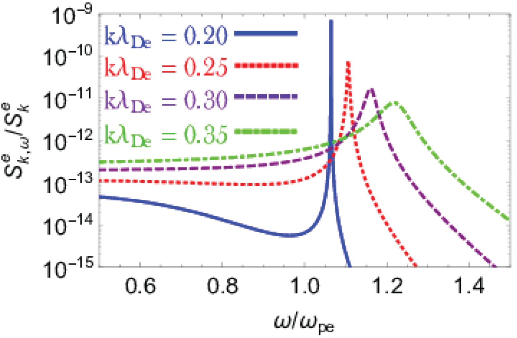Therefore, when $k\unicode[STIX]{x1D706}_{\text{De}}\ll 1$ , the electron spectral density for constant wavenumbers behaves as a delta function located at the Langmuir eigen-frequencies. As the wavenumber increases, there is a Lorentzian broadening of the Langmuir peak due to collisionless damping. For high wavenumbers, the peak keeps broadening until it is completely smoothed out, see also figure 1. It is important to emphasize that the Langmuir peak is a local but not necessarily a global maximum.

Figure 1.

The frequency dependence of the normalized spectral density of electron density fluctuations near the Langmuir resonance for varying wavenumbers. Theoretical results from (2.1). As $k\unicode[STIX]{x1D706}_{\text{De}}$ increases, the resonance broadens, the height of the peak decreases and the position of the peak shifts towards higher frequencies as dictated by the Langmuir dispersion relation $\unicode[STIX]{x1D714}^{2}=\unicode[STIX]{x1D714}_{\text{pe}}^{2}(1+3k^{2}\unicode[STIX]{x1D706}_{\text{De}}^{2})$ .

For thermal plasmas, the electron structure factor $S_{\boldsymbol{k}}^{\text{e}}=\int _{-\infty }^{+\infty }S_{\boldsymbol{k},\unicode[STIX]{x1D714}}^{\text{e}}\,\text{d}\unicode[STIX]{x1D714}$ can be analytically calculated. This quantity is also the Fourier transform of the spatial correlation function of electron density fluctuations $C_{\boldsymbol{r}}^{\text{e}}=\langle \unicode[STIX]{x1D6FF}n_{\text{e}}^{2}\rangle _{\boldsymbol{r}}$ and is the most natural choice for the normalization of $S_{\boldsymbol{k},\unicode[STIX]{x1D714}}^{\text{e}}$ . In particular, equation (2.1) can be rewritten as $S_{\boldsymbol{k},\unicode[STIX]{x1D714}}^{\text{e}}\propto \operatorname{Im}\{R_{\boldsymbol{k},\unicode[STIX]{x1D714}}\}/\unicode[STIX]{x1D714}$ where $R_{\boldsymbol{k},\unicode[STIX]{x1D714}}$ is a system response function. Such an expression allows the calculation of $S_{\boldsymbol{k}}^{\text{e}}$ with the aid of the Kramers–Kronig relations. The result reads as (Akhiezer et al. Reference Akhiezer, Akhiezer, Polovin, Sitenko and Stepanov1975)

(2.4) $$\begin{eqnarray}S_{\boldsymbol{k}}^{\text{e}}=\frac{n}{(2\unicode[STIX]{x03C0})^{3}}\frac{{\textstyle \frac{1}{2}}+k^{2}\unicode[STIX]{x1D706}_{\text{D}}^{2}}{1+k^{2}\unicode[STIX]{x1D706}_{\text{D}}}.\end{eqnarray}$$

3 Numerical method

The numerical method employed in this work for the calculation of the space–time correlation function of electron density fluctuations is based on molecular dynamics in the $(\boldsymbol{r},\boldsymbol{v})$ space using an importance sampling Monte Carlo (Tolias et al. Reference Tolias, Ratynskaia, Panarese, Longo and de Angelis2015). In contrast to Tolias et al. (Reference Tolias, Ratynskaia, Panarese, Longo and de Angelis2015) that focused on the non-interacting electron gas and the spectral densities of natural electron density fluctuations, here interactions are included. In the non-relativistic limit $|\boldsymbol{v}|\ll c$ , magnetic field generation and retardation effects are negligible. Hence, it suffices to consider only electrostatic interactions as Coulomb forces between all particle pairs. The simulation is mesh free and there is no discretization in the $(\boldsymbol{r},\boldsymbol{v})$ space.

The particle weight. Due to the high computational cost, the simulated particle density is much smaller than in the real system. Each simulated particle corresponds to a cluster of real particles. Denoting the simulation quantities with the superscript $s$ , the particle weight or scaling factor is defined by $n=wn^{\text{s}}$ or equivalently by $w=(n/N^{\text{s}})V$ with $V$ the simulation volume. In order to ensure that quantities which characterize collective plasma properties (Debye lengths, plasma frequencies, thermal velocities) are equal to those in the real system, the following scalings are applied to the electric charges, particle masses and species temperatures: $e^{\text{s}}=we$ , $m_{\unicode[STIX]{x1D6FC}}^{\text{s}}=wm_{\unicode[STIX]{x1D6FC}}$ , $T^{\text{s}}=wT$ . However, the above scalings imply that quantities which characterize collisional plasma properties such as the average electron–ion collision frequency $\bar{\unicode[STIX]{x1D708}}_{\text{ei}}\propto (ne^{4})/(\sqrt{m_{\text{e}}}T^{3/2})$ , the Coulomb radius $r_{\text{C}}\propto e^{2}/T$ and the unscreened coupling parameter $\unicode[STIX]{x1D6E4}\propto e^{2}/(n^{-1/3}T)$ differ from those in the real system. In particular, we have $\bar{\unicode[STIX]{x1D708}}_{\text{ei}}^{\text{s}}=w\bar{\unicode[STIX]{x1D708}}_{\text{ei}}$ , $r_{\text{C}}^{\text{s}}=wr_{\text{C}}$ and $\unicode[STIX]{x1D6E4}^{\text{s}}=w^{2/3}\unicode[STIX]{x1D6E4}$ . As we shall see, these effects (collisionality, large angle scattering, strong coupling) will lead to deviations from the theory.

The numerical equations of motion. The Newton equations are integrated for all simulated particles in discrete time steps with the velocity Verlet algorithm. The simulated system’s equations of motion differ from the real system’s equations of motion not only due to the introduction of the particle weight $w$ but also due to the necessity of tackling some issues caused by the discrete time step. (i) The finiteness of the integration time step introduces errors in the particle trajectories. Small errors in the particle positions can cause large errors in the particle velocities in the case of very close encounters. Particles could end up lying at mutual distances much shorter than energetically permitted, an effective source of energy that must be kept under control. We choose a simple scheme to tackle this problem, by neglecting interactions among particles at distances shorter than a fixed cutoff radius $r_{0}$ . Clearly, shorter time steps allow us to decrease the value of this numerical parameter. However, decreasing it below the simulated Coulomb radius has the adverse effect of permitting the inclusion of spurious large angle collisions. A detailed discussion on the optimal choice of this parameter is provided in § 5. (ii) Even with the introduction of $r_{0}$ , the discreteness of the integration time step still prevents the exact conservation of the total energy. In the long run, this leads to an increase of the total energy of the system. Consequently, the temperature of the simulated system does not fluctuate around its prescribed value, but slowly increases with time. The temperature is kept constant in the simulation by implementing a Nosé thermostat (Nosé Reference Nosé1984), i.e. by subjecting each particle to a frictional force $\propto \boldsymbol{v}_{i}$ . The efficiency of the thermostat is controlled via the simulation parameter $\unicode[STIX]{x1D702}$ , the value of the numerical viscosity should be large enough to maintain the prescribed average temperature and small enough to ensure that the additional dissipation does not significantly perturb the dynamics. Given the above, each simulated particle is subject to the following force:

(3.1) $$\begin{eqnarray}\displaystyle \boldsymbol{F}_{i} & = & \displaystyle -\mathop{\sum }_{j\neq i}\unicode[STIX]{x1D735}\unicode[STIX]{x1D719}_{ij}-\unicode[STIX]{x1D702}\frac{T-T_{0}}{T_{0}}\boldsymbol{v}_{i}\end{eqnarray}$$

(3.2) $$\begin{eqnarray}\displaystyle \unicode[STIX]{x1D719}_{ij} & = & \displaystyle w^{2}q_{i}q_{j}\times \left\{\begin{array}{@{}ll@{}}\displaystyle \frac{1}{|\boldsymbol{r}_{i}-\boldsymbol{r}_{j}|},\quad & \displaystyle |\boldsymbol{r}_{i}-\boldsymbol{r}_{j}|>r_{0},\\ \displaystyle \frac{1}{r_{0}},\quad & \displaystyle |\boldsymbol{r}_{i}-\boldsymbol{r}_{j}|\leqslant r_{0},\end{array}\right.\end{eqnarray}$$

where $T$ and $T_{0}$ are the instantaneous and the prescribed equilibrium temperatures, respectively.

The boundary conditions. Periodic boundary conditions are implemented as follows: (i) Concerning the particle motion, each simulated particle behaves as if the simulation volume was periodic along all three dimensions. (ii) Concerning the forces, each simulated particle feels the presence of all other simulated particles and of the periodic images of all particles (including itself) along the three dimensions, up to the nearest neighbour, i.e. 26 images.

The spectral density of fluctuations. In the simulation, the fluctuations of the electron number density $\unicode[STIX]{x1D6FF}n_{\text{e}}(\boldsymbol{r},t)=n_{\text{e}}(\boldsymbol{r},t)-n_{0}$ are sampled at discrete times on a spatial grid. For an isotropic system, it is sufficient to sample on a one-dimensional spatial grid. It is worth underlining that the spatial mesh used for the sampling does not affect the system dynamics. The sampled signal is then doubly Fourier transformed in space and time using standard fast Fourier transform (FFT) routines (Frigo & Johnson Reference Frigo and Johnson2005) and squared to get the fluctuation power spectrum. The particle weight $w$ and the sampling on a discrete mesh introduce a scaling factor so that the power spectrum from the simulation is related to that in the real system by

(3.3) $$\begin{eqnarray}S_{\boldsymbol{k},\unicode[STIX]{x1D714}}^{\text{e}}=w\frac{\unicode[STIX]{x0394}t}{N_{\text{t}}}\frac{1}{V}S_{\text{e}}^{\text{s}}(k,\unicode[STIX]{x1D714}),\end{eqnarray}$$

where $\unicode[STIX]{x0394}t$ is the interval between two successive samplings, $N_{\text{t}}$ is the number of sampled points in time and $V$ is the volume of the simulation box. The spectra are then normalized by the theoretical electron structure factor, equation (2.4). Finally, spectra obtained from multiple independent runs are averaged in order to reduce the statistical scatter. Such ensemble averaging also allows us to estimate the variance of the results.

Figure 2.

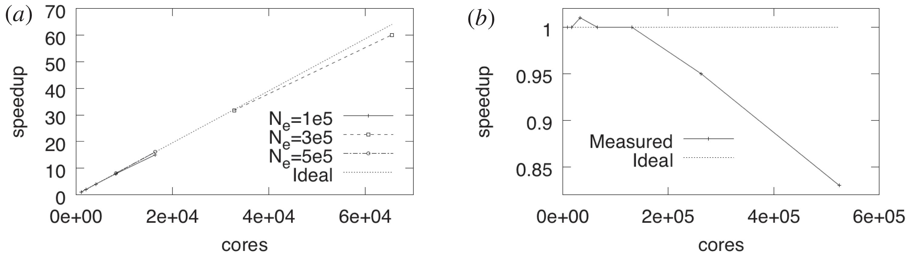
Scaling properties. (a) Strong scaling for different problem sizes. (b) Weak scaling with fixed load per node.

4 Algorithm and scalability

The computational cost is driven by the force calculations which scale as ${\sim}(N^{s})^{2}$ . As a consequence, the running time scales linearly with the number of time steps and quadratically with the number of simulated particles. The basic algorithm has been adapted to run on multi-node hardware with message passing interface (MPI) parallelization. The total number of particles is divided evenly among the MPI ranks. Each MPI rank has its own cores perform the operations on its designated chunk of particles, with the following modifications: (i) A global list of particle positions is updated after the movement step via an ALLGATHER operation. (ii) The forces acting on the particles local to the MPI rank are calculated by taking into account the influence of all particles via the global list above.

Scalability tests have been run for a small number of time steps. The code has demonstrated excellent scaling properties for the simulation parameters of interest. Figure 2(a) shows a strong scaling curve obtained on Fermi (CINECA, Italy) for different problem sizes. The scalability is excellent up to 65 536 cores (4096 nodes) and the parallel efficiency is always better than 95 %. Figure 2(b) reports the results for a weak scaling curve obtained on JuQueen (FZJ, Germany). This time the number of particles is chosen such that the load per node is constant, i.e. we have set $(N_{\text{e}}^{\text{s}})^{2}/N_{n}=10^{7}$ , where $N_{n}$ is the number of nodes (each node has 64 cores). The code again shows very good scaling capabilities. Some performance degradation can only be seen at the largest number of cores where a good parallel efficiency can be recovered with larger problem sizes (not shown here). Production runs have been carried out on Galileo (CINECA, Italy), exploiting the availability of accelerators (Intel Xeon Phi) by offloading part of the force calculation routine, which is the bottleneck of the simulation. A typical run with $N_{\text{e}}^{\text{s}}=25\,000$ and $9000$ time steps takes $15.5$ hours on 4 nodes (each node has 16 cores and 2 accelerators). Except where otherwise stated, the spectra shown here have been obtained by ensemble averaging over typically $50$ independent runs.

5 Model problem and implementation

The choice of the plasma parameters is based on restricting to fully ionized and collisionless plasmas – hence dense and hot plasmas to ensure we deal with an ideal plasma scenario. The wavenumbers are selected to reflect cases ranging from undamped Langmuir resonances to Landau damped broadened features of the spectral density of the electron density fluctuations. We thus simulate a thermal plasma consisting of electrons and protons, with the density of $n=10^{20}~\text{m}^{-3}$ and the temperature of $T=1~\text{keV}$ . The real and simulated systems have the following values for the characteristic collective parameters: $\unicode[STIX]{x1D706}_{\text{De}}=\unicode[STIX]{x1D706}_{\text{Di}}=2.35\times 10^{-5}~\text{m}$ , $\unicode[STIX]{x1D714}_{\text{pe}}=5.6\times 10^{11}~\text{rad}~\text{s}^{-1}$ and $\unicode[STIX]{x1D714}_{\text{pi}}=1.3\times 10^{10}~\text{rad}~\text{s}^{-1}$ , while the real system has the following values for the characteristic collisional parameters: $r_{\text{C}}=1.44\times 10^{-12}~\text{m}$ , $\unicode[STIX]{x1D6E4}=10^{-5}$ and $\bar{\unicode[STIX]{x1D708}}_{\text{ei}}=1.5\times 10^{5}~\text{s}^{-1}$ . The smallest wavenumber investigated in this work is $k=10^{4}~\text{m}^{-1}$ and corresponds to $k\unicode[STIX]{x1D706}_{\text{De}}=0.235$ . The simulation domain, unless stated otherwise, is a cubic box of dimension $L=2\unicode[STIX]{x03C0}\times 10^{-4}~\text{m}=26.73~\unicode[STIX]{x1D706}_{\text{De}}$ .

Figure 3.

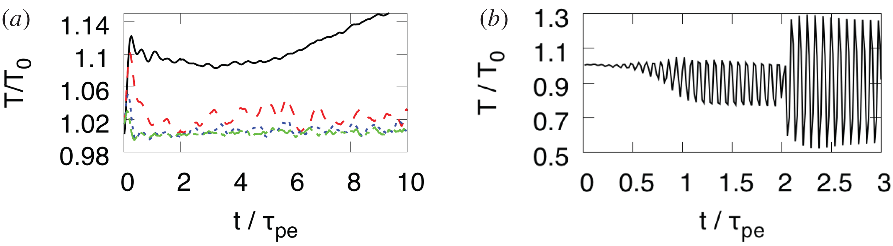
Time evolution of the electron temperature for different values of the viscosity. (a) Black: $\unicode[STIX]{x1D702}=10^{-20}$ , red: $\unicode[STIX]{x1D702}=10^{-19}$ , blue: $\unicode[STIX]{x1D702}=5\,\times \,10^{-19}$ , green: $\unicode[STIX]{x1D702}=10^{-18}$ ; (b) $\unicode[STIX]{x1D702}=5\,\times \,10^{-18}$ .

The numerical viscosity. As mentioned, a thermostat has been introduced in order to prevent a rise in the temperature of the simulated system. We therefore investigated the impact of this artificial viscosity on the simulation results. Figure 3(a,b) illustrates the temporal profiles of the system temperature for $N_{\text{e}}^{\text{s}}=5000$ and different values of the numerical viscosity $\unicode[STIX]{x1D702}$ that governs the thermostat efficiency. Apart from an initial transient, the system exhibits a steady behaviour. 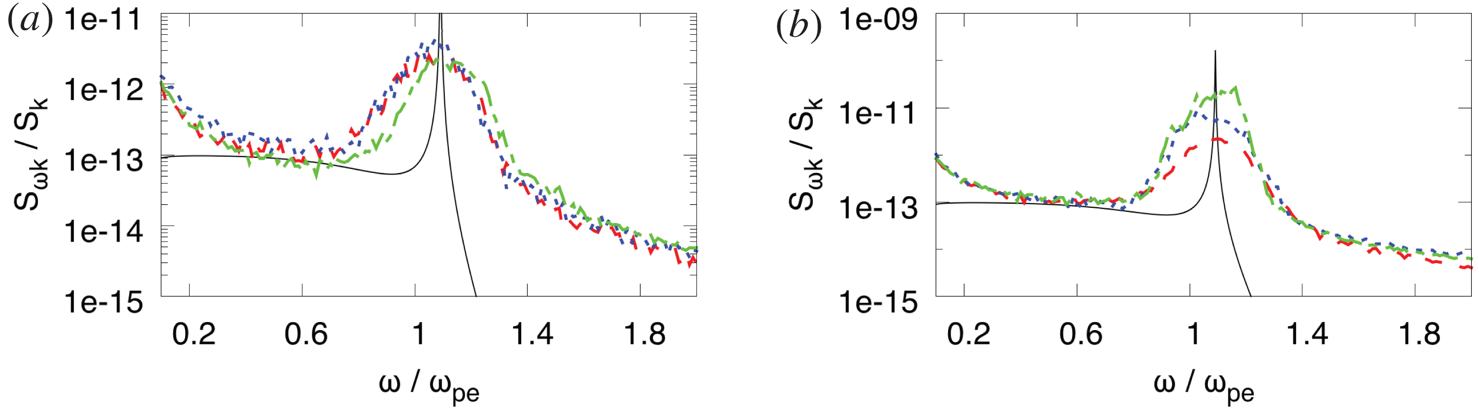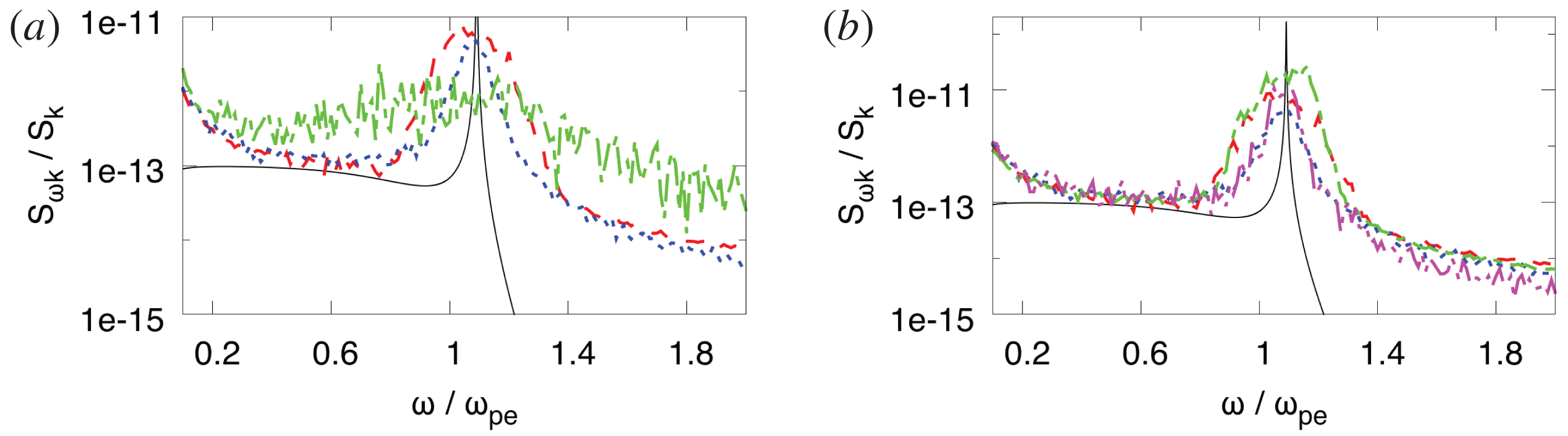Small values of $\unicode[STIX]{x1D702}$ result to a system temperature deviating from the prescribed temperature – see the black line in figure 3(a), whereas large values of $\unicode[STIX]{x1D702}$ essentially drive the particle dynamics – see figure 3(b). In this latter case, also the resulting spectrum is affected, as demonstrated in figure 4(a). We have drawn the conclusion that the value $\unicode[STIX]{x1D702}=10^{-19}$ gives the best compromise for our model problem. Hence, this value is employed in all the simulations that follow.

Figure 4.

Spectral densities of electron density fluctuations for $k=10^{4}~\text{m}^{-1}$ , $r_{0}=1.0~\unicode[STIX]{x1D706}_{\text{De}}$ . (a) Dependence on the value of the viscosity. Black: theory, red: $\unicode[STIX]{x1D702}=10^{-20}$ , blue: $\unicode[STIX]{x1D702}=10^{-19}$ , green: $\unicode[STIX]{x1D702}=5\times 10^{-18}$ . (b) Dependence on the number of simulated particles. Black: theory, red: $N_{\text{e}}^{\text{s}}=5000$ , blue: $N_{\text{e}}^{\text{s}}=25\,000$ , green: $N_{\text{e}}^{\text{s}}=75\,000$ .

The boundary conditions. In order to assess the impact of the adopted boundary conditions, the charge distribution in the simulations has been investigated. For an ideal plasma, the electrostatic potential around an elementary point charge is $\unicode[STIX]{x1D719}(r)=(e/r)\exp (-r/\unicode[STIX]{x1D706}_{\text{D}})$ . Within the linearized Boltzmann relation, the stationary ion and electron densities around this test charge will be $n_{\text{i}}(r)=n[1-e\unicode[STIX]{x1D719}(r)/T]$ and $n_{\text{e}}(r)=n[1+e\unicode[STIX]{x1D719}(r)/T]$ , respectively. This results in a net charge profile

(5.1) $$\begin{eqnarray}\displaystyle q(r)/e=4\unicode[STIX]{x03C0}\int _{0}^{r}x^{2}[n_{\text{i}}(x)-n_{\text{e}}(x)]\,\text{d}x=-1+\left(1+\frac{r}{\unicode[STIX]{x1D706}_{\text{D}}}\right)\text{e}^{-r/\unicode[STIX]{x1D706}_{\text{D}}}. & & \displaystyle\end{eqnarray}$$

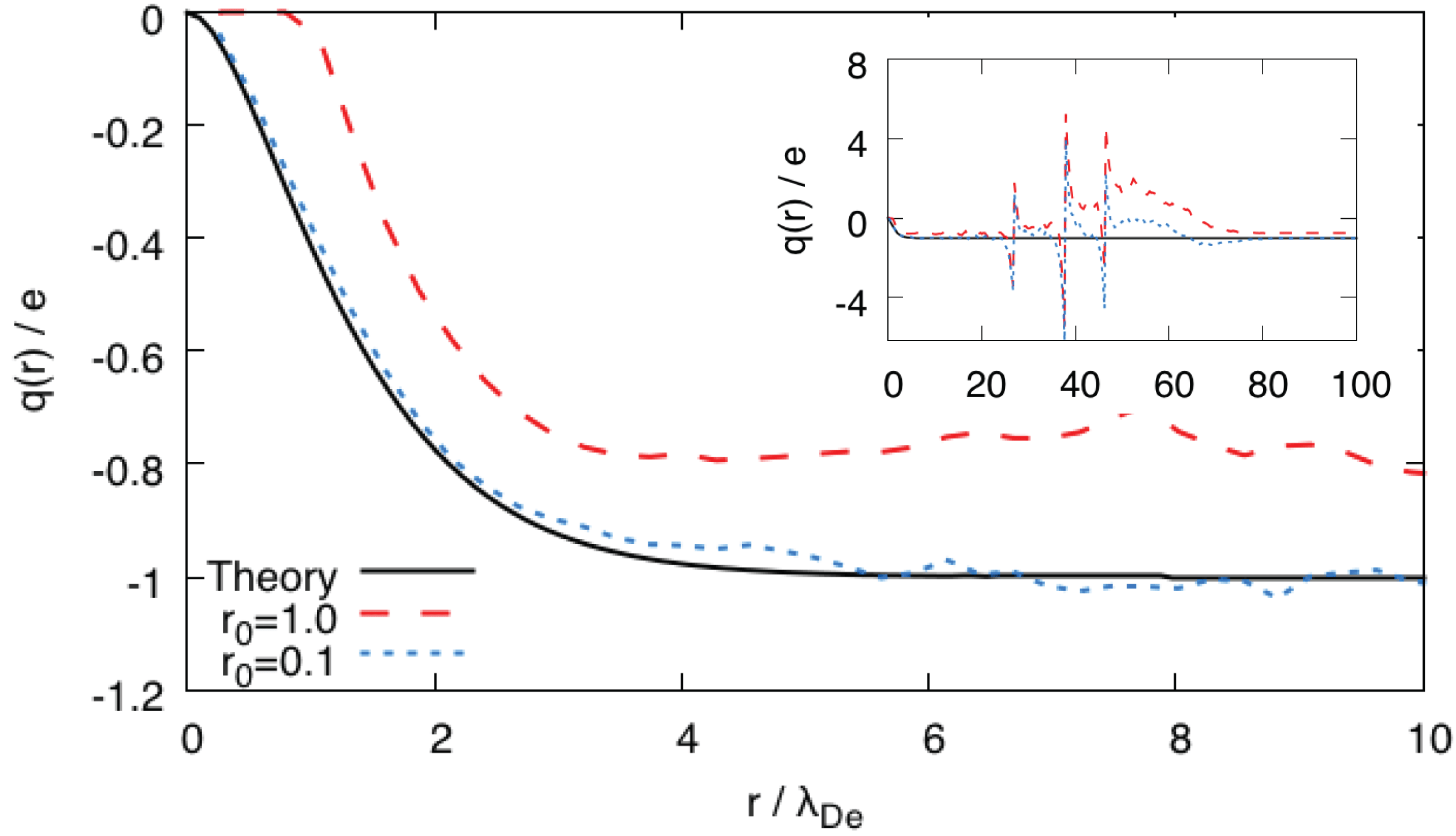
Figure 5 shows results on the average net charge around a positive test charge as obtained in simulations with $N_{\text{e}}^{\text{s}}=5000$ , $r_{0}=1.0~\unicode[STIX]{x1D706}_{\text{De}}$ or $r_{0}=0.1~\unicode[STIX]{x1D706}_{\text{De}}$ . Simulation results are compared to the theoretical result, equation (5.1). We conclude that the agreement is very good already for $r_{0}\leqslant 0.1~\unicode[STIX]{x1D706}_{\text{De}}$ . The periodic boundary conditions introduce a discontinuous behaviour in the charge distribution at distances corresponding to the simulation box dimensions – see the inset of figure 5, but this does not affect the fluctuation spectra at the shorter wavelengths, as we shall see in what follows.

Figure 5.

Net charge cumulative distribution around a positive test charge: comparison of the $r_{0}=1.0~\unicode[STIX]{x1D706}_{\text{De}}$ and $r_{0}=0.1~\unicode[STIX]{x1D706}_{\text{De}}$ cases with the theoretical result for $N_{\text{e}}^{\text{s}}=5000$ . The simulation box is a cube of dimension $L=26.73~\unicode[STIX]{x1D706}_{\text{De}}$ .

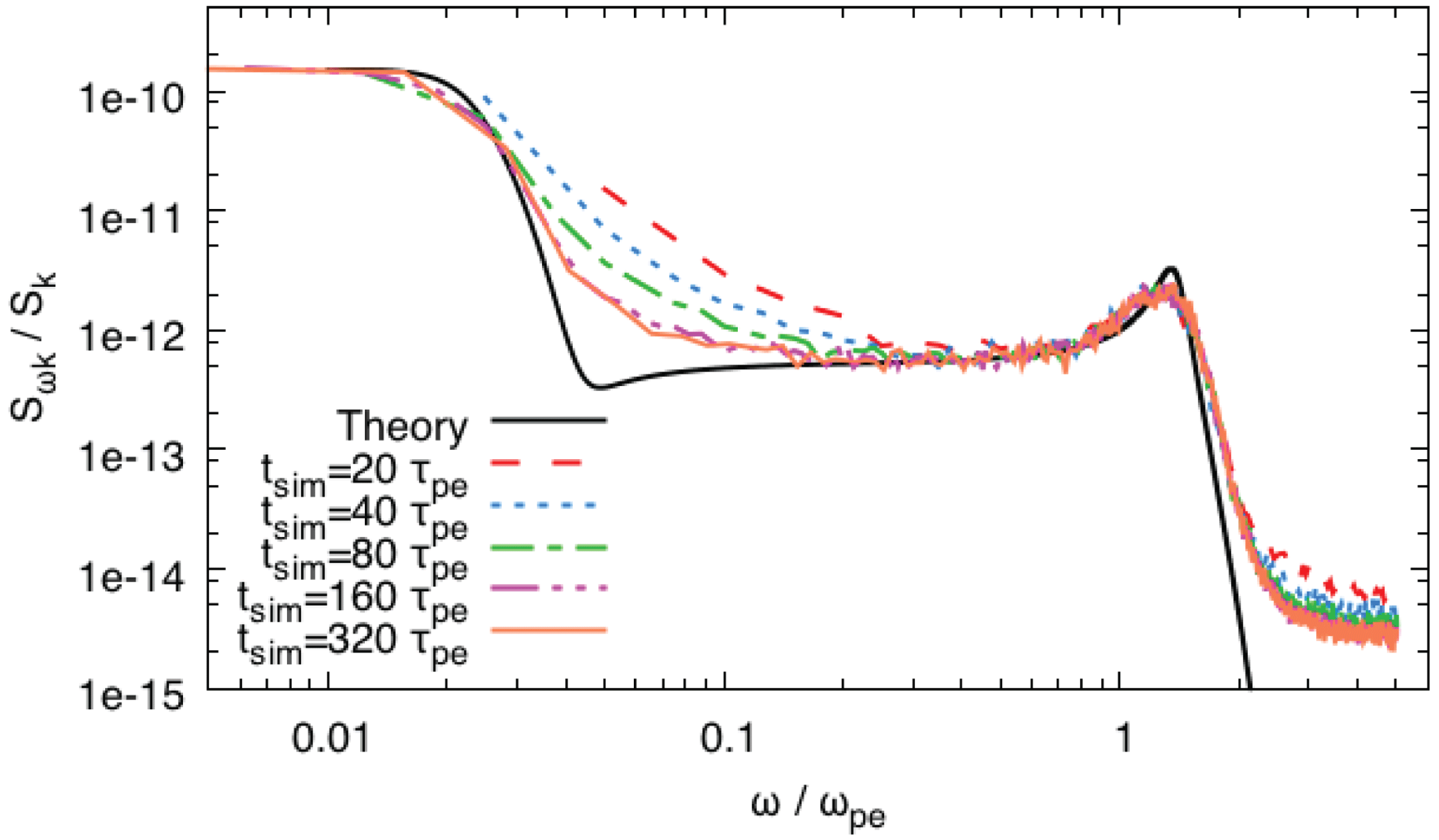
The simulation duration. It is important to discern the minimum value for the simulation duration that suffices for an adequate resolution of the Langmuir spectral feature and its vicinity. It is convenient to express the simulation time in terms of the electron plasma period $\unicode[STIX]{x1D70F}_{\text{pe}}=2\unicode[STIX]{x03C0}/\unicode[STIX]{x1D714}_{\text{pe}}$ . Figure 6 displays the fluctuation power spectra as obtained by simulations with $N_{\text{e}}^{\text{s}}=5000$ , $r_{0}=1.0~\unicode[STIX]{x1D706}_{\text{De}}$ and varying $t_{\text{sim}}$ values. We observe the following: (i) It is evident that $t_{\text{sim}}<80\unicode[STIX]{x1D70F}_{\text{pe}}$ leads to noticeably distorted spectra. The simulation results in the vicinity of the Langmuir mode have essentially converged for $t_{\text{sim}}\geqslant 80\unicode[STIX]{x1D70F}_{\text{pe}}$ and only small improvements can be gained by performing longer simulations. (ii) As expected, it is demonstrated that longer simulation times allow us to capture physics relevant for lower frequencies. It is worth noting that the simulations correctly reproduce the part of the spectrum that arises from the ion dynamics. (iii) At very high frequencies the simulated spectra reach a lower bound. The intensity of the background noise is determined by the time step, with shorter time steps resulting in lower background.

Figure 6.

Spectral densities of electron density fluctuations for $k=2\times 10^{4}~\text{m}^{-1}$ , $r_{0}=1.0~\unicode[STIX]{x1D706}_{\text{De}}$ , $N_{\text{e}}^{\text{s}}=5000$ and varying values of the simulation duration $t_{\text{sim}}$ .

The number of simulated particles. An increase of the particle number leads to a decrease of the particle weight $w$ and implies that the simulated system approaches the real system also as far as collisional aspects are concerned. Therefore, the effect of the simulated particle number on the numerical power spectra has been investigated. Figure 4(b) shows results for $r_{0}=1.0~\unicode[STIX]{x1D706}_{\text{De}}$ . Increasing the number of particles leads to an almost linear improvement of the Langmuir peak height, whereas the peak width is almost unaffected.

The numerical cutoff. We shall explore the role of the cutoff radius $r_{0}$ on the numerical power spectra. Linear fluctuation theory (see § 2) neglects large amplitude fluctuations induced by collisions that occur at distances shorter than the Coulomb radius. As discussed in § 4, the simulated Coulomb radius depends on the number of simulated particles through the particle weight. This suggests that the numerical cutoff should always be chosen to be larger than $r_{\text{C}}^{\text{s}}$ . Figure 7(a), where results for $N_{\text{e}}^{\text{s}}=25\,000$ – corresponding to $r_{\text{C}}^{\text{s}}=0.3~\unicode[STIX]{x1D706}_{\text{De}}$ – and different values for $r_{0}$ are compared to the theoretical spectrum for $k=10^{4}~\text{m}^{-1}$ , supports this conclusion. The agreement with the theoretical spectra improves by reducing $r_{0}$ , but only as long as the condition $r_{0}>r_{\text{C}}^{\text{s}}$ is satisfied. For cutoff values $r_{0}<r_{\text{C}}^{\text{s}}$ , large angle collisions are included in the simulation that appreciably distort the numerical power spectrum. Therefore, the optimal value is close to $r_{0}=r_{\text{C}}^{\text{s}}$ . Figure 7(b) compares results obtained with different simulated particle numbers and different cutoff radii $r_{0}$ . We notice that it is this parameter that mainly affects the width of the simulated peak.

Figure 7.

Spectral densities of electron density fluctuations for $k=10^{4}~\text{m}^{-1}$ . The cutoff radius, $r_{0}$ , is expressed in $\unicode[STIX]{x1D706}_{\text{De}}$ units. (a)  $N_{\text{e}}^{\text{s}}=25\,000$ . Black: theory, red: $r_{0}=1.0$ , blue: $r_{0}=0.1$ , green: $r_{0}=0.01$ . (b) Results obtained with different simulated particle numbers and different cutoff radii. Black: theory, red: $N_{\text{e}}^{\text{s}}=25\,000$ , $r_{0}=1.0$ , blue: $N_{\text{e}}^{\text{s}}=25\,000$ , $r_{0}=0.1$ , green: $N_{\text{e}}^{\text{s}}=75\,000,~r_{0}=1.0$ , magenta: $N_{\text{e}}^{\text{s}}=50\,000,~r_{0}=0.1$ .

6 Numerical results

Having explored the dependence on the main simulation parameters, we shall now present numerical results obtained with the most computationally demanding simulation performed. The time step is $\text{d}t=0.01~\unicode[STIX]{x1D70F}_{\text{pe}}$ and the numerical cutoff is $r_{0}=0.1~\unicode[STIX]{x1D706}_{\text{De}}$ . The simulation domain is a cubic box of dimension $L=26.7~\unicode[STIX]{x1D706}_{\text{De}}$ , and $N_{\text{e}}^{\text{s}}=25\,000$ is employed. The latter parameters lead to a particle weight $w\simeq 10^{6}$ . As a consequence:

1. (i) The electron–ion collision frequency is $\bar{\unicode[STIX]{x1D708}}_{\text{ei}}^{\text{s}}\simeq 2.2\times 10^{10}~\text{s}^{-1}\simeq 0.04\unicode[STIX]{x1D714}_{\text{pe}}$ , which implies that the excess collisionality of the simulated system cannot shift the position of the Langmuir mode but can broaden the width of the spectral density maximum for wavenumbers that correspond to weak Landau damping.

2. (ii) The coupling parameter is $\unicode[STIX]{x1D6E4}^{\text{s}}\simeq 0.1$ and the normalized screening parameter is $\unicode[STIX]{x1D705}^{\text{s}}\simeq 0.8$ , which implies that the simulated system is non-ideal but still weakly coupled (Hamaguchi, Farouki & Dubin Reference Hamaguchi, Farouki and Dubin1996), the excess coupling cannot displace the Langmuir mode but it can influence the width of the spectral density maximum.

3. (iii) The Coulomb radius is $r_{\text{C}}^{\text{s}}\simeq 1.43\times 10^{-6}~\text{m}\simeq 0.06\unicode[STIX]{x1D706}_{\text{De}}$ , $r_{0}>r_{\text{C}}^{\text{s}}$ ensures that large angle scattering is removed from the simulations but it also implies that short distance binary collisions are neglected, which is again most likely to affect the width of the spectral density maximum.

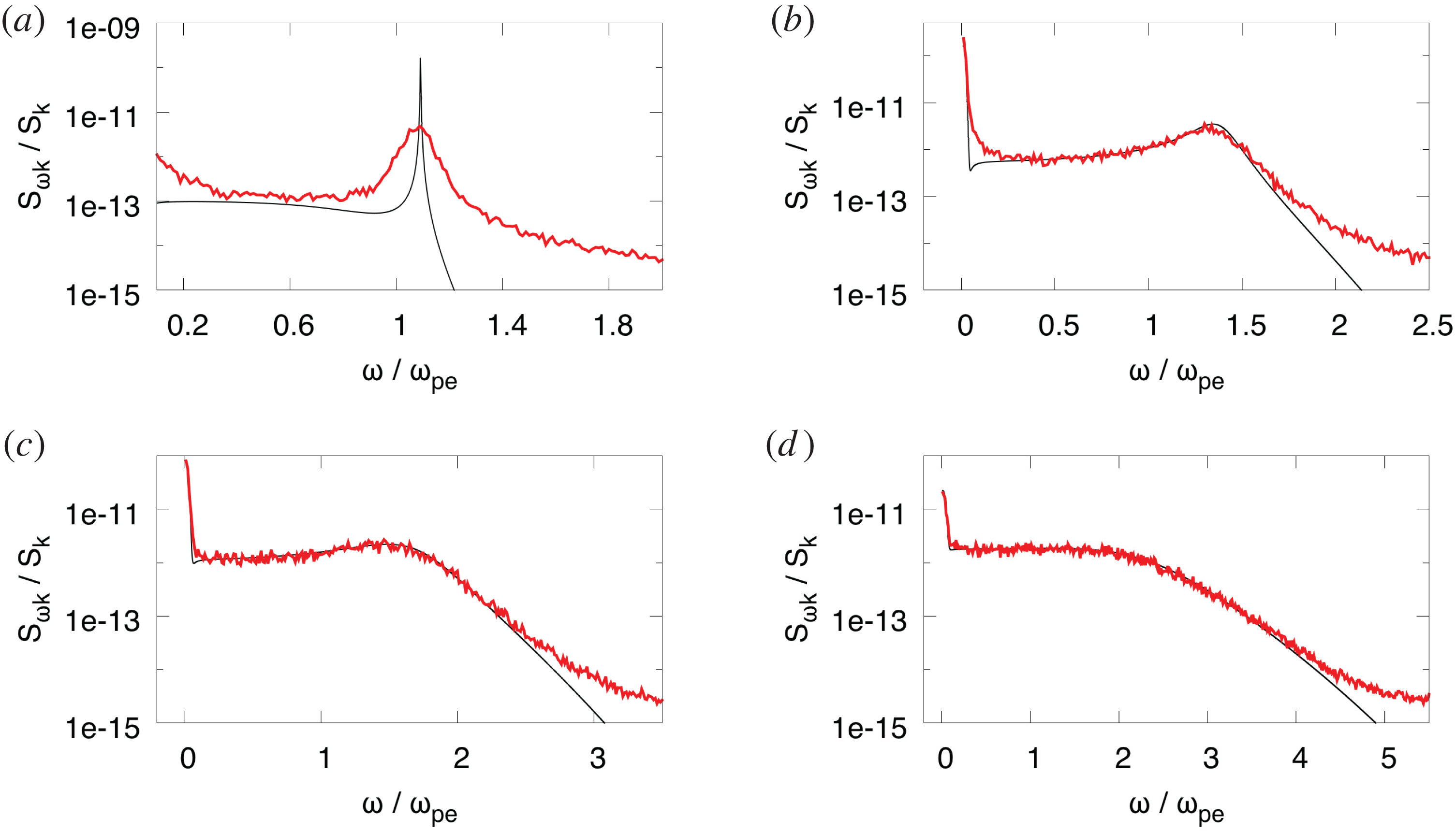
The power spectra for different wavelengths are presented in figure 8. The agreement with the theoretical results is excellent up to $k\unicode[STIX]{x1D706}_{\text{De}}\gtrsim 0.5$ for the chosen simulation parameters that imply a cutoff radius $r_{0}=0.1\,\unicode[STIX]{x1D706}_{\text{De}}$ , i.e. six orders of magnitude larger than the Coulomb radius of the real system. At those wavelengths, the effect of Landau damping overcomes the combined effect of excess collisionality and coupling. Note also how the agreement extends well below the electron plasma frequency, down to $0.01~\unicode[STIX]{x1D714}_{pe}$ where the ion dynamics is starting to contribute. At the smaller wavenumber, the excess collisionality of the MD simulation produces noticeable broadening of the Langmuir peak. The agreement can be extended towards the long wavelength limit, $k\unicode[STIX]{x1D706}_{\text{De}}\ll 1$ , (where the Langmuir peak becomes a delta function) by increasing the number of simulated particles, although at a high computational cost.