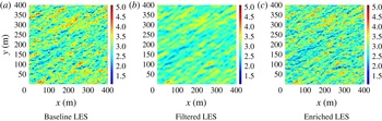
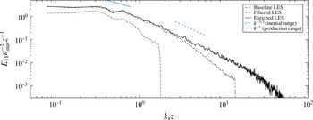
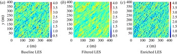
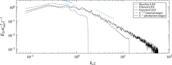
1 Introduction
In a recent review paper, He, Jin & Yang (Reference He, Jin and Yang2017) emphasized the need for accurate modelling of the dynamic coupling between the spatial and temporal scales of motion in large eddy simulations of turbulence-generated noise and particle laden turbulence. This is also a critically important requirement in environmental applications such as pollution dispersion in the planetary boundary layer (PBL) and fatigue loading in wind turbines that operate within the PBL. Prior research in structural modelling for large eddy simulation (LES) has resulted in several interesting numerical techniques, where the focus of modelling is on explicit evaluation of subgrid scales (see Sagaut, Deck & Terracol Reference Sagaut, Deck and Terracol2013). Most methods invariably involve introducing auxiliary computational meshes that are embedded within the primary LES grids. Scotti & Meneveau (Reference Scotti and Meneveau1999) introduced a deterministic and computationally efficient method of reconstructing subgrid fluctuations on a finer mesh using fractal interpolation, based on geometric considerations. Flohr & Vassilicos (Reference Flohr and Vassilicos2000) present a technique to synthesize incompressible, isotropic and stationary velocity fields based on kinematic simulation (KS) ideas first introduced by Fung et al. (Reference Fung, Hunt, Malik and Perkins1992). As a simple kinematic simulation that reproduces isotropic energy spectrum for scales at higher wavenumbers, they demonstrated this method for passive tracer dispersion in isotropic turbulence. While this approach bears some similarities with the methodology introduced in this paper, their approach fails to capture any direct energy transfers between scales since the Fourier modes are essentially frozen and also restricted to isotropic box turbulence problems. Domaradzki & Loh (Reference Domaradzki and Loh1999) have proposed several procedures for estimating the subgrid fields. In their approach the subgrid production term is integrated over a time interval parameterized using the characteristic turnover time of the subgrid fields. While their approach provides a relatively cheap technique to evaluate the subgrid terms, it requires computation of an approximate inverse filter. Other techniques based on solutions to dynamical systems such as the chaotic map model of Mukerji et al. (Reference Mukerji, Mcdonougha, Mengüç, Manickavasagam and Chung1998) have also been used to approximate subgrid fluctuations. Other higher fidelity simulation techniques that have become popular in recent years include the multilevel simulations such as the variational multiscale method (VMS) developed by Hughes et al. (Reference Hughes, Feijóo, Mazzei and Quincy1998) and the Terracol, Sagaut & Basdevant (Reference Terracol, Sagaut and Basdevant2003) multilevel algorithm (TMA). While these techniques are similar to traditional multigrid algorithms for steady state calculations, they are computationally quite expensive since they are based on solution to exact Navier–Stokes equations on embedded computational grids. However, they tend to be cheaper than direct numerical simulations since they rely on freezing (via the quasi-static approximation) high frequency content (represented on the finer embedded grids) over some time interval defined by the chosen cycling strategy. Multiscale simulation algorithms for LES using wavelets, such as the stochastic coherent adaptive large eddy simulation (SCALES) method (see Stefano & Vasilyev Reference Stefano and Vasilyev2013), have also been recently developed. In this method, the separation between resolved and unresolved fields is obtained by wavelet threshold filtering. Since their algorithm is based on the idea of explicit filtering, they achieve grid-independent solutions by refining the wavelet collocation grids while controlling the spectral resolution via thresholding. Other methods that rely on overlapping grids that attempt to resolve multiple scales have also been developed for certain specific applications in geophysics. The one-way coupling algorithm of Khanna & Brasseur (Reference Khanna and Brasseur1997) uses a fine grid located near the wall in order to capture the smaller length scales that are under-resolved by the primary LES grid. In their simulations, the two grids are independently integrated; the only means of coupling is in the form of a velocity matching Dirichlet boundary condition on the finer grid, and a rescaling of the subgrid viscosity at the boundaries. A two-way coupled version of this technique has also been independently developed by Sullivan, McWilliams & Moeng (Reference Sullivan, McWilliams and Moeng1996), which was further modified by Manhart & Friedrich (Reference Manhart and Friedrich1999) for DNS of separated turbulent boundary layers. The multiscale techniques discussed above all suffer from either one or more of the following three drawbacks which limit their usability in more realistic flow problems. The methods (i) are applicable only for highly idealized problems such as homogeneous isotropic turbulence and are unable to capture the physics behind local energy transfer and inter-scale interactions, (ii) are limited in spectral resolution of the reconstructed scales; this is particularly true of the models that use deconvolution based on truncated series representation of the inverse filter operator, to reconstruct the resolvable subfilter scales and are traditionally used to obtain subfilter-scale closures in LES equations (Stolz & Adams Reference Stolz and Adams1999) and (iii) require significant computational overhead since these methods are designed to solve either full or some elements of the complete governing equations on embedded domains. Hence, their competitiveness is generally appraised in comparison with costs and accuracy associated with DNS.
The multiscale simulation strategy discussed herein attempts to address each of the three drawbacks. The overall framework has three components: (i) a nonlinear rapid disortion theory (RDT) model using the Gabor transform along with successive filtering to generate scale separation, (ii) representation of subfilter fields via a small number of random/discrete modes transformed to physical space using non-uniform fast Fourier transforms (NUFFT) and (iii) LES using a robust subgrid-scale model, which allows for large-scale inhomogeneities. The principal idea behind our simulation strategy is the localized nature of small-scale features, which allows for their representation using wavepackets obtained via Gabor transform. The Gabor transform has been used previously (Nazarenko, Kevlahan & Dubrulle Reference Nazarenko, Kevlahan and Dubrulle1999, Reference Nazarenko, Kevlahan and Dubrulle2000; Dubrulle et al. Reference Dubrulle, Laval, Nazarenko and Kevlahan2001) to study canonical irrotational strain and pure shear flow problems to analytically study the role played by small-scale turbulence in shear reduction in larger scales. They have also used the WKB-RDT formulation to compute the exact mean shear profile (two-dimensional case), in full agreement with the classical results by Oberlack (Reference Oberlack2001). More recently, Dubrulle et al. (Reference Dubrulle, Laval, Sullivan and Werne2002) used the WKB-RDT formulation to construct a dynamical subgrid-scale model and analytical profiles for the planetary surface layer. The only previous use of WKB-RDT in subfilter-scale enrichment is by Laval, Dubrulle & Nazarenko (Reference Laval, Dubrulle and Nazarenko2004) where they developed a numerical algorithm (particle in cell) to evolve subfilter-scale fields in a numerically efficient manner for two-dimensional decaying and forced isotropic turbulence. The present development is inspired by these previous efforts and provides a method for physics-based fine-scale enrichment of LES fields which is also cost effective.
2 The subfilter kinematic simulation
2.1 Gabor transform and the assumption of quasi-homogeneity
We first introduce some terminology which is required to concretely describe our approach. Kinematic simulation, as envisioned in Fung et al. (Reference Fung, Hunt, Malik and Perkins1992), corresponds to synthesis of a velocity field
 $\boldsymbol{u}$
over a region
 $(\boldsymbol{x},t)\in \unicode[STIX]{x1D6FA}(\mathbb{R}^{3},[0,\infty ))$
, using a series expansion:
 $$\begin{eqnarray}\boldsymbol{u}(\boldsymbol{x},t)=\mathop{\sum }_{n=1}^{N}[\boldsymbol{a}_{n}(t)\exp (\text{i}\boldsymbol{k}_{n}(t)\boldsymbol{\cdot }\unicode[STIX]{x1D73B}(\boldsymbol{x},t))]\end{eqnarray}$$
such that the finite number of Fourier modes,
 $(\boldsymbol{a}_{n}(t),\boldsymbol{k}_{n}(t))$
capture all the relevant (time evolving) scales present in the velocity field. While such a Fourier sum can capture features such as anisotropy and spatio-temporal correlations, it is implicitly limited to homogeneous flows with spatially non-varying statistics. However, wall-bounded high Reynolds number flows exhibit significant inhomogeneity (see Jiménez Reference Jiménez2011), especially in the wall-normal direction due to kinematic and dynamic effects imposed by the no-penetration and no-slip wall. As such a Fourier decomposition (2.1) has limited applicability in wall-bounded flows.
The Gabor transform provides a mathematical framework to localize the Fourier expansion given in (2.1). The Gabor transform of a velocity field
 $\boldsymbol{u}(\boldsymbol{x})$
is defined as
 $$\begin{eqnarray}\hat{u} _{i}(\boldsymbol{x}_{0},\boldsymbol{k})=\int _{\boldsymbol{x}\in \mathbb{R}^{3}}u_{i}(\boldsymbol{x})f(\unicode[STIX]{x1D700}(\boldsymbol{x}_{0}-\boldsymbol{x}))\exp (\text{i}\boldsymbol{k}(t)\boldsymbol{\cdot }(\boldsymbol{x}_{0}-\boldsymbol{x}))\,\text{d}\boldsymbol{x}.\end{eqnarray}$$
Note that in this definition, the function
 $f(\boldsymbol{x})$
is typically a compact support window function (
 $\in \mathbb{C}_{c}^{\infty }$
) similar to those used in defining distributions. The scalar parameter,
 $\unicode[STIX]{x1D700}$
controls the effective support of the window function,
 $f(\boldsymbol{x})$
and is relevant for introducing scale separation. The windowing restricts the variability of the inhomogeneous field
 $\boldsymbol{u}(\boldsymbol{x},t)$
defined over a large domain
 $\unicode[STIX]{x1D6FA}(\mathbb{R}^{3})$
to a smaller region
 $\unicode[STIX]{x1D712}(\mathbb{R}^{3})\subset \unicode[STIX]{x1D6FA}(\mathbb{R}^{3})$
where one can make an assumption of quasi-homogeneity or local homogeneity. The velocity field can be reconstructed using the exact inverse transform (see appendix C) given as,
 $$\begin{eqnarray}u_{i}(\boldsymbol{x})=\frac{1}{(2\unicode[STIX]{x03C0})^{3}f(0)}\int _{k\in \mathbb{R}^{3}}\hat{u} _{i}(\boldsymbol{x},\boldsymbol{k})\,\text{d}\boldsymbol{k}.\end{eqnarray}$$
It is important to acknowledge that the shifted transform defined in (2.2) results in an inverse that does not depend on
 $\unicode[STIX]{x1D700}$
or on the choice of the window function,
 $f(\boldsymbol{x})$
, since this information is embedded in the Gabor modes,
 $\hat{u} _{i}$
. Once the Gabor transform (or Gabor modes in a discrete sense),
 $\hat{u} _{i}(\boldsymbol{x},\boldsymbol{k})$
is known (or synthesized), its inversion does not require further specification of the window function,
 $f(x)$
or the scale separation parameter,
 $\unicode[STIX]{x1D700}$
, since the scalar factor
 $f(0)$
can be absorbed without loss of generality. The underlying idea behind the LES enrichment discussed in this paper is the synthesis of the Fourier–Gabor modes
 $\hat{u} _{i}(\boldsymbol{x})$
for
 $\boldsymbol{x}\in \unicode[STIX]{x1D712}(\mathbb{R}^{3})$
which is a smaller subdomain (or a quasi-homogeneous region) inside the full problem domain,
 $\unicode[STIX]{x1D6FA}(\mathbb{R}^{3})$
. The notion of scale separation (via the parameter
 $\unicode[STIX]{x1D700}$
) is used to seek a local expansion (within each subdomain) such as the one given in (2.1) as a discrete representation for the integral inverse in (2.3). The two expressions are asymptotically equivalent in the vanishing limit of
 $\unicode[STIX]{x1D700}$
(see appendix C). Furthermore, the discrete expansion in (2.1), which can be evaluated using fast algorithms, is particularly convenient due to the band-limited nature of velocity field
 $u_{i}$
. By defining the window function as
 $f(\unicode[STIX]{x1D700}(\boldsymbol{x}_{0}-\boldsymbol{x}))$
, we can control the windowing region depending on the scales present in the field. This scale separation requirement can be mathematically stated as
 $\text{supp}[f(\unicode[STIX]{x1D700}(\boldsymbol{x}_{0}-\boldsymbol{x}))]\gg 2\unicode[STIX]{x03C0}/k$
which should be true for all
 $k$
in (2.1). More precisely, as
 $\unicode[STIX]{x1D700}$
decreases, the support of the window function increases, and if the support of the window function is much larger than the largest scale present in field
 $\boldsymbol{u}$
, the discrete decomposition given in (2.1) becomes more accurate.
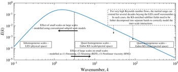
The multiscale decomposition of the velocity field over three scales and the modelled interactions.

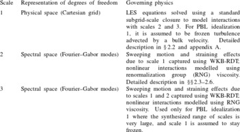
Description of the governing physics for the three scales under the multiscale decomposition shown in figure 1. Note that each enriched scale shown in figure 1 spans approximately 3–4 decades. When the desired enrichment bandwidth is larger than 3–4 decades, a multiple band of enriched scales is required as was the case in PBL idealization 1.

We thus have the following two restrictions on size of the subdomain (later termed a quasi-homogeneous region),
 $\unicode[STIX]{x1D712}(\mathbb{R}^{3})$
: (i) it must be substantially larger than length scale of the largest eddy enriched in it (this follows from the requirement that
 $\unicode[STIX]{x1D700}\ll 1$
) and (ii) it cannot be too large, otherwise the quasi-homogeneous assumption (discussed in § 2.3) may be violated for the flow problem being considered. These two restrictions require the decomposition of the velocity field as superposition of velocity fields of different scales, and sufficiently accurate modelling of interactions amongst scales. Figure 1 illustrates this decomposition where the velocity field is decomposed over three different scales. Further details regarding the treatment of the three scales is provided in table 1. We can thus write the velocity,
 $u_{i}$
at a particular location,
 $x_{i}\in \unicode[STIX]{x1D6FA}(\mathbb{R}^{3})$
and time,
 $t$
as
 $$\begin{eqnarray}u_{i}(x_{j},t)=u_{i}^{(1)}(x_{j},t)+u_{i}^{(2)}(x_{j},t)+u_{i}^{(3)}(x_{j},t).\end{eqnarray}$$
Note that the velocity at a particular scale can be obtained using a successive filtering procedure
 $$\begin{eqnarray}\displaystyle & \displaystyle u_{i}^{(1)}(x_{j},t)=\int _{\unicode[STIX]{x1D6FA}(\mathbb{R}^{3}),\unicode[STIX]{x1D70F}\in \mathbb{R}}G^{(1)}(x_{j}-r_{j},t-\unicode[STIX]{x1D70F})u_{i}(r_{j},\unicode[STIX]{x1D70F})\,\text{d}\boldsymbol{r}\,\text{d}\unicode[STIX]{x1D70F} & \displaystyle\end{eqnarray}$$
 $$\begin{eqnarray}\displaystyle & \displaystyle u_{i}^{(2)}(x_{j},t)=\left[\int _{\unicode[STIX]{x1D6FA}(\mathbb{R}^{3}),\unicode[STIX]{x1D70F}\in \mathbb{R}}G^{(2)}(x_{j}-r_{j},t-\unicode[STIX]{x1D70F})u_{i}(r_{j},\unicode[STIX]{x1D70F})\,\text{d}\boldsymbol{r}\,\text{d}\unicode[STIX]{x1D70F}\right]-u_{i}^{(1)}(x_{j},t) & \displaystyle\end{eqnarray}$$
 $$\begin{eqnarray}\displaystyle & \displaystyle u_{i}^{(3)}(x_{j},t)=u_{i}(x_{j},t)-(u_{i}^{(1)}(x_{j},t)+u_{i}^{(2)}(x_{j},t)), & \displaystyle\end{eqnarray}$$
where the filter kernels,
 $G^{k}$
have transfer functions with wider supports at each successive filtering procedure. (The wider support here refers to that of the physical space filter function
 $G(\boldsymbol{x})$
. The wider support here refers to that of physical space filter function
 $G(x)$
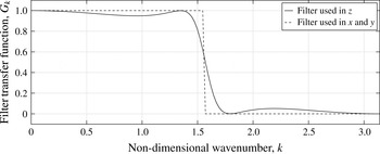
; duality of the Fourier transform correspondingly implies a smaller bandwidth in spectral space. The spectral space transfer functions for the filters used in all included simulations are given in figure 2. Note that since the vertical direction is not periodic, a boundary modification is needed. The boundary filter used by Tritschler et al. (Reference Tritschler, Olson, Lele, Hickel, Hu and Adams2014) for filtering their localized artificial diffusivity (LAD) term (Gaussian filter), is used at the boundaries.
Transfer functions of the filters used in vertical (
 $z$
) and horizontal (
 $x$
–
 $y$
plane) directions. The filter used in
 $z$
is the compromise filter used by Spyropoulos & Blaisdell (Reference Spyropoulos and Blaisdell1996) which combines an explicit least squares filter and a compact difference filter by Lele (Reference Lele1992).

In the algorithm introduced in this paper, the largest scales given by
 $u_{i}^{(1)}$
are evaluated using a standard large eddy simulation. The finer scales present in
 $u^{(2)}$
and
 $u^{(3)}$
are enriched using the kinematic simulation. Note that in practice, the finest scale, scale 3 is only required if the LES enrichment is expected to enhance the spectral bandwidth by several decades in wave space. In those cases, it is prudent to further decompose the enriched field into two scales and consider the interactions between the two enriched scales (see figure 1). This three-scale decomposition is used in PBL idealization 1, and could be potentially used in problems where the largest scales (scale 1) are computed using hydrostatic general climate models (not studied in this paper), where virtually all the turbulence would need to be synthesized using the KS enrichment.
The solution to entire velocity field,
 $u_{i}(x_{j},t)$
requires the modelling of the following interactions: (i) interactions between
 $u_{i}^{(1)}(x_{j},t)$
and
 $u_{i}^{(2)}(x_{j},t)$
and (ii) interactions between
 $u_{i}^{(2)}(x_{j},t)$
and
 $u_{i}^{(3)}(x_{j},t)$
. The convective nonlinearity in the governing equations implies that the dynamic interaction amongst the scales is in general two-way coupled. These interactions are implicitly captured in traditional simulations since the entire velocity field
 $u_{i}$
is evolved on a numerical grid that is finer than the Nyquist requirements of the smallest scales present in
 $u^{(3)}$
. We can further classify the interactions between the two adjacent bins into two categories (i) the local interactions which occur between two wavenumbers of similar size (near the edges of the wavenumber bins in figure 1 and (ii) the distant interactions that involve wavenumbers not close to the filter edges.
As will be shown later in § 2.3, the Gabor transform and the WKB-RDT formulation is used to model the forward cascade component of the distant interactions (the F-type interactions according to the classification by Waleffe Reference Waleffe1992). The quasi-homogeneous assumption implied in using RDT, implicitly captures the nonlinearity associated with the pressure (non-local in physical space) via the projection operator,
 $((k_{i}k_{j}/k_{m}k_{m})-\unicode[STIX]{x1D6FF}_{ij})$
. The effect of nonlinear interactions amongst modes within the same decomposition/bin, as well as the local interactions (in relative terms) associated with adjacent decompositions/bins, are modelled using a spectral viscosity that comes from renormalization group (RNG) theory. The backward cascade component of the distant interactions (the R-type interactions according to Waleffe’s classification) are not modelled (except for scale 1) since the present formulation only considers one-way coupling. For the largest scale (scale 1 in figure 1) which is governed by a standard LES algorithm, the effects of scales 2 and 3 are indeed modelled using a traditional subgrid closure model as discussed in § 2.2.
To facilitate the derivation of the governing equations and their reduction to obtain the modelled equations used for scale enrichment, we further define the following velocity fields,
 $$\begin{eqnarray}U_{i}^{(1)}(x_{j},t)=\int _{\unicode[STIX]{x1D6FA}(\mathbb{R}^{3}),\unicode[STIX]{x1D70F}\in \mathbb{R}}T^{(1)}(x_{j}-r_{j},t-\unicode[STIX]{x1D70F})u_{i}(r_{j},\unicode[STIX]{x1D70F})\,\text{d}\boldsymbol{r}\,\text{d}\unicode[STIX]{x1D70F}\end{eqnarray}$$
and
 $$\begin{eqnarray}U_{i}^{(2)}(x_{j},t)=\int _{\unicode[STIX]{x1D6FA}(\mathbb{R}^{3}),\unicode[STIX]{x1D70F}\in \mathbb{R}}T^{(2)}(x_{j}-r_{j},t-\unicode[STIX]{x1D70F})u_{i}(r_{j},\unicode[STIX]{x1D70F})\,\text{d}\boldsymbol{r}\,\text{d}\unicode[STIX]{x1D70F},\end{eqnarray}$$
where
 $T^{(i)}$
is a filter with a width (in physical space) larger than that of
 $G^{(i)}$
, and
 $r$
and
 $\unicode[STIX]{x1D70F}$
are dummy variables of integration. They correspond to the physical space coordinate and time, respectively. In practice, we have observed that using a filter for
 $T$
with a width twice that of
 $G$
is sufficient to obtain the desired scale separation, and all applications discussed henceforth in this paper use this definition for the filter
 $T$
. We can now also define residual velocity fields as
 $$\begin{eqnarray}U_{i}^{(1)r}(x_{j},t)=u_{i}^{(1)}(x_{j},t)-U_{i}^{(1)}(x_{j},t)\end{eqnarray}$$
and
 $$\begin{eqnarray}U_{i}^{(2)r}(x_{j},t)=(u_{i}^{(1)}(x_{j},t)+u_{i}^{(2)}(x_{j},t))-U_{i}^{(2)}(x_{j},t).\end{eqnarray}$$
Finally, note that the quasi-homogeneous regions described in earlier are directly related to the multiscale decomposition. For example, the velocity field in the intermediate scale (scale 2), can be described over a quasi-homogeneous region,
 $\unicode[STIX]{x1D712}(\mathbb{R}^{3})$
that extends over the filter width of
 $T^{(1)}$
(as opposed to
 $G^{(1)}$
) which satisfies both the scale separation requirement and the quasi-homogeneity requirements on
 $\unicode[STIX]{x1D712}(\mathbb{R}^{3})$
.
2.2 Equations for superfilter/resolved/large scales
The largest scales (scale 1 in figure 1, denoted as
 $(U_{i},\unicode[STIX]{x1D6E9})$
for clarity) are evaluated in physical space using a conventional LES, where the governing equations are
 $$\begin{eqnarray}\displaystyle & \displaystyle \unicode[STIX]{x2202}_{t}U_{i}+U_{j}\unicode[STIX]{x2202}_{j}U_{i}=-\unicode[STIX]{x2202}_{i}P-\unicode[STIX]{x2202}_{j}\unicode[STIX]{x1D70F}_{ij}^{d}+\unicode[STIX]{x1D6FF}_{ij}g_{j}\left[\frac{\unicode[STIX]{x1D6E9}-\unicode[STIX]{x1D6E9}_{0}}{\unicode[STIX]{x1D6E9}_{0}}\right]+2\unicode[STIX]{x1D700}_{ijk}\unicode[STIX]{x1D6FA}_{j}(G_{k}-U_{k})+\unicode[STIX]{x1D708}\unicode[STIX]{x2202}_{j}\unicode[STIX]{x2202}_{j}U_{i} & \displaystyle\end{eqnarray}$$
 $$\begin{eqnarray}\displaystyle & \displaystyle \unicode[STIX]{x2202}_{t}\unicode[STIX]{x1D6E9}+U_{j}\unicode[STIX]{x2202}_{j}\unicode[STIX]{x1D6E9}=-\unicode[STIX]{x2202}_{j}q_{j}+\unicode[STIX]{x1D705}\unicode[STIX]{x2202}_{j}\unicode[STIX]{x2202}_{j}\unicode[STIX]{x1D703}. & \displaystyle\end{eqnarray}$$
Here,
 $G_{k}$
is a geostrophic wind speed (causing an effective constant pressure gradient forcing),
 $\unicode[STIX]{x1D70F}_{ij}^{d}$
is the deviatoric part of the residual stress tensor defined as
 $\unicode[STIX]{x1D70F}_{ij}=\widetilde{u_{i}u_{j}}-U_{i}U_{j}$
where
 $\tilde{(\cdot )}$
is the filter applied at scale 1 (
 $G^{(1)}$
). Similarly,
 $q_{j}$
is the residual flux given as
 $q_{j}=\widetilde{\unicode[STIX]{x1D703}u_{j}}-U_{j}\unicode[STIX]{x1D6E9}$
. The scalar field
 $P$
is the modified large scale pressure (which includes
 $1/3$
trace of the SGS tensor), and
 $g_{j}$
is the acceleration due to gravity. The subgrid model used for the residual stresses along with the numerical algorithms, boundary and initial conditions is discussed in appendix A in some detail.
2.3 Modelled equations for subfilter scales
We now discuss the derivations and modelling of the evolution equations for the Fourier–Gabor modes for an intermediate scale (scale 2) which describe the velocity field,
 $u^{(2)}$
over a subdomain
 $x\in \unicode[STIX]{x1D712}(\mathbb{R}^{3})$
. For simplicity of notation, we will denote the velocity field at scale 2 as
 $\boldsymbol{u}$
, the large-scale component of scale 1 (
 $U^{(1)}$
) as
 $\boldsymbol{U}$
and the residual component of scale 1 (
 $\boldsymbol{U}^{(1)r}$
) as
 $\boldsymbol{U}^{r}$
. Note that under the quasi-homogeneous assumption we can claim
 $\unicode[STIX]{x2202}_{j}U_{i}=\text{const.}$
over the subdomain,
 $x\in \unicode[STIX]{x1D712}(\mathbb{R}^{3})$
.
The equations governing subfilter scales can be derived by simply subtracting the filtered Navier–Stokes equations (see (2.12) and (2.13)) from the full Navier–Stokes equations:
 $$\begin{eqnarray}\displaystyle \unicode[STIX]{x2202}_{t}u_{i}+U_{j}\unicode[STIX]{x2202}_{j}u_{i} & = & \displaystyle -\unicode[STIX]{x2202}_{i}p-u_{j}\unicode[STIX]{x2202}_{j}U_{i}-\unicode[STIX]{x2202}_{j}(u_{i}u_{j})-\unicode[STIX]{x2202}_{j}(u_{i}U_{j}^{r})-\unicode[STIX]{x2202}_{j}(U_{i}^{r}u_{j})\nonumber\\ \displaystyle & & \displaystyle +\,\unicode[STIX]{x1D708}\unicode[STIX]{x2202}_{j}\unicode[STIX]{x2202}_{j}u_{i}+\unicode[STIX]{x2202}_{j}\unicode[STIX]{x1D70F}_{ij}^{d}+\unicode[STIX]{x1D6FF}_{ij}g_{j}\frac{\unicode[STIX]{x1D703}}{\unicode[STIX]{x1D6E9}_{0}}-2\unicode[STIX]{x1D716}_{ijk}\unicode[STIX]{x1D6FA}_{j}u_{k}\end{eqnarray}$$
and
 $$\begin{eqnarray}\unicode[STIX]{x2202}_{t}\unicode[STIX]{x1D703}+U_{j}\unicode[STIX]{x2202}_{j}\unicode[STIX]{x1D703}=-u_{j}\unicode[STIX]{x2202}_{j}\unicode[STIX]{x1D6E9}-\unicode[STIX]{x2202}_{j}(U_{j}^{r}\unicode[STIX]{x1D703})-\unicode[STIX]{x2202}_{j}(u_{j}\unicode[STIX]{x1D6E9}^{r})-\unicode[STIX]{x2202}_{j}(u_{j}\unicode[STIX]{x1D703})+\unicode[STIX]{x2202}_{j}q_{j}+\unicode[STIX]{x1D705}\unicode[STIX]{x2202}_{j}\unicode[STIX]{x2202}_{j}\unicode[STIX]{x1D703}.\end{eqnarray}$$
Depending on the filter used in
 $T^{1}$
, we can define two parameters, (i) the filter width (or the subdomain)
 $\unicode[STIX]{x1D712}(\mathbb{R}^{3})$
and (ii) the turnover time scale,
 $\unicode[STIX]{x1D70F}$
of the superfilter field,
 $U_{i}$
. Under the assumption of quasi-homogeneity, we can now make the following simplifications.
-
(i) Split the superfilter field: (note that since the field
 $U_{i}$
is band-limited due to application of the filter
$T^{1}$
, the truncated Taylor series is not an unreasonable interpolation over a region smaller (or of the same size) than the filter width. The exact field can be reconstructed using the sinc-interpolation.) (2.16)
$$\begin{eqnarray}\displaystyle U_{i}(x_{i})=U_{i}^{0}+x_{j}\unicode[STIX]{x2202}_{j}U_{i}|^{0},\quad x\in \unicode[STIX]{x1D712}(\mathbb{R}^{3}). & & \displaystyle\end{eqnarray}$$
-
(ii) Galilean transform to the sweeping frame:
(2.17)
$$\begin{eqnarray}\displaystyle \left.\begin{array}{@{}c@{}}\displaystyle \tilde{t}=t\\ \tilde{x}_{i}=x_{i}-U_{i}^{0}t,\quad t\in [0,\unicode[STIX]{x1D70F}].\end{array}\right\} & & \displaystyle\end{eqnarray}$$


Equations (2.14) and (2.15) can now be significantly simplified to obtain
 $$\begin{eqnarray}\displaystyle \unicode[STIX]{x2202}_{\tilde{t}}u_{i}+(x_{m}\unicode[STIX]{x2202}_{m}U_{j})\unicode[STIX]{x2202}_{j}u_{i} & = & \displaystyle -\unicode[STIX]{x2202}_{i}p-u_{j}\unicode[STIX]{x2202}_{j}U_{i}-\unicode[STIX]{x2202}_{j}(u_{i}u_{j})-\unicode[STIX]{x2202}_{j}(u_{i}U_{j}^{r})-\unicode[STIX]{x2202}_{j}(U_{i}^{r}u_{j})\nonumber\\ \displaystyle & & \displaystyle +\,\unicode[STIX]{x1D708}\unicode[STIX]{x2202}_{j}\unicode[STIX]{x2202}_{j}u_{i}+\unicode[STIX]{x2202}_{j}\unicode[STIX]{x1D70F}_{ij}^{d}+\unicode[STIX]{x1D6FF}_{ij}g_{j}\frac{\unicode[STIX]{x1D703}}{\unicode[STIX]{x1D6E9}_{0}}-2\unicode[STIX]{x1D716}_{ijk}\unicode[STIX]{x1D6FA}_{j}u_{k}\end{eqnarray}$$
and
 $$\begin{eqnarray}\unicode[STIX]{x2202}_{\tilde{t}}\unicode[STIX]{x1D703}+(x_{m}\unicode[STIX]{x2202}_{m}U_{j})\unicode[STIX]{x2202}_{j}\unicode[STIX]{x1D703}=-u_{j}\unicode[STIX]{x2202}_{j}\unicode[STIX]{x1D6E9}-\unicode[STIX]{x2202}_{j}(U_{j}^{r}\unicode[STIX]{x1D703})-\unicode[STIX]{x2202}_{j}(u_{j}\unicode[STIX]{x1D6E9}^{r})-\unicode[STIX]{x2202}_{j}(u_{j}\unicode[STIX]{x1D703})+\unicode[STIX]{x2202}_{j}q_{j}+\unicode[STIX]{x1D705}\unicode[STIX]{x2202}_{j}\unicode[STIX]{x2202}_{j}\unicode[STIX]{x1D703}\end{eqnarray}$$
for
 $\boldsymbol{x}\in \unicode[STIX]{x1D712}(\mathbb{R}^{3})$
and
 $\tilde{t}\in [0,\unicode[STIX]{x1D70F}]$
. The material derivative term implied by the left-hand side suggests the use of a time-dependent wavenumber, so that the Fourier–Gabor modes of an arbitrary scalar field (say
 $\unicode[STIX]{x1D719}(x,t)$
) following the larger scales do not change with time in the sweeping frame
 $\tilde{x}(t)$
, given in (2.17). In other words, we seek time dependent
 $\boldsymbol{k}(t)$
such that
 $D\unicode[STIX]{x1D719}(\tilde{x},\tilde{t})/D\tilde{t}=0\leftrightarrow \text{d}\hat{\unicode[STIX]{x1D719}}(\boldsymbol{k},\tilde{t})/\text{d}t=0$
, and hence the wave vectors must be constrained by an eikonal (ray-tracing) equation. Thus, we can now derive the governing equations for the Fourier–Gabor modes (
 $\boldsymbol{k}_{m}$
,
 $\boldsymbol{a}_{n}$
,
 $\hat{\unicode[STIX]{x1D703}}$
) in the sweeping frame to obtain
 $$\begin{eqnarray}\displaystyle & \displaystyle \frac{\text{d}a_{i}}{\text{d}\tilde{t}}=\left(\frac{2k_{i}k_{m}}{k^{2}}-\unicode[STIX]{x1D6FF}_{im}\right)a_{j}\unicode[STIX]{x2202}_{j}U_{m}+\left(\frac{k_{i}k_{j}}{k^{2}}-\unicode[STIX]{x1D6FF}_{ij}\right)g_{j}\unicode[STIX]{x1D6FD}\hat{\unicode[STIX]{x1D703}}-\unicode[STIX]{x1D708}k^{2}a_{i}+\hat{f}_{i}^{\bot }+{\hat{h}}_{i}^{\bot } & \displaystyle\end{eqnarray}$$
 $$\begin{eqnarray}\displaystyle & \displaystyle \frac{\text{d}\hat{\unicode[STIX]{x1D703}}}{\text{d}\tilde{t}}=-a_{j}\unicode[STIX]{x2202}_{j}\unicode[STIX]{x1D6E9}-\unicode[STIX]{x1D705}k^{2}\hat{\unicode[STIX]{x1D703}}+\hat{f}_{\unicode[STIX]{x1D703}}+{\hat{h}}_{\unicode[STIX]{x1D703}}, & \displaystyle\end{eqnarray}$$
with the eikonal equation given as
 $$\begin{eqnarray}\frac{\text{d}k_{i}}{\text{d}\tilde{t}}=-k_{j}\unicode[STIX]{x2202}_{i}U_{j},\end{eqnarray}$$
where
 $\hat{f}_{i}$
represents the Fourier projection of source term
 $\unicode[STIX]{x2202}_{j}\unicode[STIX]{x1D70F}_{ij}$
on the wave vector
 $k_{i}$
and
 $\hat{f}_{i}^{\bot }=((k_{i}k_{j}/k^{2})-\unicode[STIX]{x1D6FF}_{ij})\hat{f}_{j}$
. Similarly, the term
 ${\hat{h}}_{i}^{\bot }$
comes from the nonlinear terms
 $\unicode[STIX]{x2202}_{j}(u_{i}u_{j})+\unicode[STIX]{x2202}_{j}(U_{i}^{r}u_{j})+\unicode[STIX]{x2202}_{j}(u_{i}U_{j}^{r})$
. The simplest model for the nonlinear terms is a spectral eddy viscosity such as the one obtained using RNG (see Canuto & Dubovikov Reference Canuto and Dubovikov1996; Laval, Dubrulle & Nazarenko Reference Laval, Dubrulle and Nazarenko2001). Under this modelling assumption, we compute
 ${\hat{h}}_{i}^{\bot }$
and
 ${\hat{h}}_{\unicode[STIX]{x1D703}}$
as
 $$\begin{eqnarray}{\hat{h}}_{i}^{\bot }=-\unicode[STIX]{x1D708}_{t}(k)k^{2}a_{i},\quad {\hat{h}}_{\unicode[STIX]{x1D703}}=-\frac{\unicode[STIX]{x1D708}_{t}(k)}{Pr}k^{2}\hat{\unicode[STIX]{x1D703}},\end{eqnarray}$$
where the RNG model (isotropic turbulence) for the spectral viscosity is given as:
 $$\begin{eqnarray}\unicode[STIX]{x1D708}_{t}(k)=\left(\unicode[STIX]{x1D708}^{2}+0.02\int _{k}^{\infty }q^{-2}E(q)\,\text{d}q\right)^{1/2}-\unicode[STIX]{x1D708}.\end{eqnarray}$$
The energy spectrum,
 $E(k)$
in (2.24) is estimated using the Fourier–Gabor modes
 $(k_{i},a_{i})$
. This is consistent with the assumptions and findings reported in Laval et al. (Reference Laval, Dubrulle and Nazarenko2001) where comparisons with DNS of three-dimensional isotropic turbulence suggest that a simple turbulent viscosity model is sufficient to obtain accurate decay rates. We further note that in the subgrid scale (SGS) model of Dubrulle et al. (Reference Dubrulle, Laval, Sullivan and Werne2002), the authors ignore this term entirely by arguing that the subgrid–subgrid interactions are negligible. However, in our implementation we have noticed that the absence of the spectral viscosity (and the implied time scale), leads to non-physical increase in energy at high wavenumbers inconsistent with the
 $5/3$
rule. This is consistent with the observations made by Laval et al. (Reference Laval, Dubrulle and Nazarenko2001) for isotropic turbulence, where they argue that the role of the local interactions in the nonlinear term is to weaken the intense vortices caused by the non-local interactions. The turbulent viscosity model based on RNG is a natural choice for regularization desired in this formulation, since it gives the desired
 $k^{-4/3}$
scaling for
 $\unicode[STIX]{x1D708}_{t}$
as
 $k\rightarrow \infty$
and
 $k^{0}$
scaling as
 $k\rightarrow 0$
.
As is demonstrated in § 3, the use of this simple isotropic spectral viscosity is sufficient to obtain correct second-order space–time statistics. Finally, note that the nonlinear terms,
 ${\hat{h}}_{\unicode[STIX]{x1D703}}$
and
 $\hat{f}_{\unicode[STIX]{x1D703}}$
are related to
 ${\hat{h}}_{i}$
and
 $\hat{f}_{i}$
respectively using a turbulent Prandtl number taken to be 0.65. This assumption is natural since the closure model for both
 $\hat{f}_{i}$
and
 ${\hat{h}}_{i}$
uses a viscosity (the
 $\unicode[STIX]{x1D70F}_{ij}$
term that appears in
 $\hat{f}_{i}$
is typically modelled by the LES code using an eddy viscosity).
2.4 Initialization and quenching of discrete Fourier–Gabor modes
The Fourier–Gabor modes are initialized in different subdomains within the coarse LES domain using the mean (averaged along homogeneous directions) profiles. Denoting the mean profiles for the velocity and potential temperatures as
 $\overline{u}_{i}$
and
 $\overline{\unicode[STIX]{x1D703}}$
respectively, we construct the anisotropic initial modes by again leveraging the RDT hypothesis for an incompressible Boussinesq fluid and distort randomly sampled isotropic modes. However, such an RDT linearization is invalid since the mean shear observed in the log-law region of the PBL is typically small compared to the turbulent time scales. This inconsistency is remedied by making use of Mann’s eddy lifetime (see Mann Reference Mann1994) hypothesis where the isotropic random modes are distorted through a wavenumber-dependent eddy lifetime given as:
 $$\begin{eqnarray}\unicode[STIX]{x1D70F}(k)\propto \frac{1}{k\sqrt{\displaystyle \int _{k}^{\infty }E(k)\,\text{d}k}}\;\Longrightarrow \;\unicode[STIX]{x1D70F}(k)\unicode[STIX]{x1D64E}=c_{\unicode[STIX]{x1D70F}}(kL)^{-2/3}\left[\text{}_{2}F_{1}\left(\frac{1}{3},\frac{17}{6};\frac{4}{3};-(kL)^{-2}\right)\right]^{-1/2},\end{eqnarray}$$
where
 $\unicode[STIX]{x1D64E}$
is the Frobenius norm of
 $\text{d}\overline{U}_{i}/\text{d}x_{j}$
tensor and
 $c_{\unicode[STIX]{x1D70F}}$
is a constant. Its evaluation/calibration is discussed in appendix B for problems which are statistically stationary and homogeneous in two directions. However, note that, in principle, this constant can be computed dynamically (for non-stationary, highly inhomogeneous problems) by matching the turbulent kinetic energy in a newly defined overlap region which comprises of wavenumbers that make up the smallest LES resolved fields and the largest KS enriched fields. However, since the primary focus of this paper is limited to LES of PBL, this dynamic procedure will be the focus of a later study. Recent work by Segalini & Arnqvist (Reference Segalini and Arnqvist2015) extends Mann’s lifetime model for stratified flows by incorporating additional physics at time scales corresponding to the Brunt–Vaisala frequency. However, note that in their paper, they attempt to model the spectral tensor (instead of the velocity modes). It is possible to decompose the spectral tensor (square root decomposition) to obtain the velocity modes but an analytical decomposition is not possible for problems with a general gradient tensor
 $\unicode[STIX]{x2202}U_{i}/\unicode[STIX]{x2202}x_{j}$
. While one can use the Cholesky decomposition to numerically decompose the spectral tensor, this approach is susceptible to round-off and numerical error associated with numerical evaluation of the RDT equations and leads to the spectral tensors that are not guaranteed to be positive semi-definite. Nevertheless, we note that since the modification to Mann’s model made by Segalini & Arnqvist (Reference Segalini and Arnqvist2015) only affects the low wavenumbers (
 $kL<1$
) the two models are essentially equivalent in the present application since in the present approach the large scales (low wavenumbers) are resolved using conventional LES. Finally, note that while alternate choices for the eddy lifetime model are available (see discussion in Mann Reference Mann1994), and were evaluated as part of this work, the model in (2.25) was adjudged to be the most accurate at capturing the anisotropy of the enriched small scales. While eddy lifetime models based on RNG or eddy-damped quasi-normal Markovian result in smaller values of the shear constant (
 $c_{\unicode[STIX]{x1D70F}}$
), they tend to generate small scales that are inherently more oblate than the predictions made by solving the full nonlinear governing equations, and hence were not used for the purpose of initializing the enriched fields.
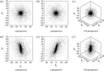
Figures (d–f) show the wavenumbers corresponding to the initialized field in a single quasi-homogeneous region located at
 $z=5~\text{m}$
for PBL idealization 2 (see § 5). Parts (a–c) show the corresponding random wavenumbers sampled on isotropic shells as part of the pre-initialization.

The initial condition for the enriching KS is obtained by rapid distortion of isotropic turbulence. This pre-initialization isotropic turbulence is synthesized by random sampling of wave vectors on spherical shells with radii (wavenumbers) that are logarithmically spaced to allow for efficient sampling of turbulence, which has an inherent power-law behaviour in spectral space (see figure 3). The turbulent kinetic energy and turbulent potential energy spectra used are given in (2.26). The values of the constants,
 $\unicode[STIX]{x1D6FC}$
and
 $\unicode[STIX]{x1D6FD}$
are taken to be 1.7 (corresponding to the Kolmogorov constant) and 0.8 (see Chougule, Mann & Kelly Reference Chougule, Mann and Kelly2013) respectively.
 $$\begin{eqnarray}\displaystyle E(k)=\unicode[STIX]{x1D6FC}\unicode[STIX]{x1D700}^{2/3}L^{5/3}\frac{(kL)^{4}f_{\unicode[STIX]{x1D702}}(k\unicode[STIX]{x1D702})}{[1+(kL)^{2}]^{17/6}},\quad S(k)=\unicode[STIX]{x1D6FD}\unicode[STIX]{x1D700}^{-1/3}\unicode[STIX]{x1D700}_{\unicode[STIX]{x1D703}}L^{5/3}\frac{(kL)^{2}}{[1+(kL)^{2}]^{11/6}}. & & \displaystyle\end{eqnarray}$$
The representative length scale,
 $L$
is a length scale that is computed using either the LES (as done in PBL idealization 2), or is simply specified as a length scale proportional to distance from the surface (as done in PBL idealization 1). (While there is some ambiguity regarding choice of
 $L$
, it is rather inconsequential since its choice is compensated by the value of
 $c_{\unicode[STIX]{x1D70F}}$
which is computed directly. By computing
 $L$
using the LES fields, we obtain
 $L\propto z$
which ensures that the kinetic energy supplied by the enriching KS fields decreases as the distance from the wall increases in a manner that is consistent with the increase in the kinetic energy resolved by the LES.) The dissipation range spectrum denoted by
 $f_{\unicode[STIX]{x1D702}}(k\unicode[STIX]{x1D702})$
is taken to be a simple exponential decay of the following form (see Pope Reference Pope2000):
 $$\begin{eqnarray}f_{\unicode[STIX]{x1D702}}(k\unicode[STIX]{x1D702})=\exp [-\unicode[STIX]{x1D6FD}_{\unicode[STIX]{x1D702}}k\unicode[STIX]{x1D702}]=\exp [-\unicode[STIX]{x1D6FD}_{\unicode[STIX]{x1D702}}kL(\unicode[STIX]{x1D702}/L)],\end{eqnarray}$$
where the Kolmogorov length scale is defined as
 $\unicode[STIX]{x1D702}=(\unicode[STIX]{x1D708}^{3}/\unicode[STIX]{x1D700})^{1/4}$
, and the decay constant,
 $\unicode[STIX]{x1D6FD}_{\unicode[STIX]{x1D702}}$
can be shown to be
 $[2\unicode[STIX]{x1D6FC}\unicode[STIX]{x1D6E4}(4/3)]^{3/4}$
(derived using the constraint
 $\unicode[STIX]{x1D700}=\int _{0}^{\infty }2\unicode[STIX]{x1D708}k^{2}E(k)\,\text{d}k$
, along with the assumption
 $\unicode[STIX]{x1D702}^{2}/L^{2}\ll 1$
). The PBL flows being considered in this paper tend to be at an asymptotically infinite Reynolds number, and since
 $\unicode[STIX]{x1D702}/L\propto Re^{-3/4}$
, it is reasonable to assume that
 $\unicode[STIX]{x1D702}/L\rightarrow 0$
for such flows. However, for the finite Reynolds number channel flow being considered in this paper, the ratio
 $\unicode[STIX]{x1D702}/L$
is
 $O(10^{-2})$
, and hence the dissipation range spectrum,
 $f_{\unicode[STIX]{x1D702}}(k\unicode[STIX]{x1D702})$
plays an important role in KS enrichment at finite Reynolds numbers.
The dissipation rates are computed by assuming a local equilibrium between the rates of production and dissipation of the turbulent kinetic and potential energy (2.28)
 $$\begin{eqnarray}\displaystyle \unicode[STIX]{x1D700}=-\langle u^{\prime }w^{\prime }\rangle \frac{\text{d}\overline{U}}{\text{d}z}-\langle v^{\prime }w^{\prime }\rangle \frac{\text{d}\overline{V}}{\text{d}z}+\frac{g}{\unicode[STIX]{x1D703}}\langle w^{\prime }\unicode[STIX]{x1D703}^{\prime }\rangle ,\quad \unicode[STIX]{x1D700}_{\unicode[STIX]{x1D703}}=-\langle w^{\prime }\unicode[STIX]{x1D703}^{\prime }\rangle \frac{\text{d}\overline{\unicode[STIX]{x1D6E9}}}{\text{d}z}. & & \displaystyle\end{eqnarray}$$
The spectral viscosity closure for the nonlinear term in (2.20) (closure model in (2.24)) corresponds to a decay of total energy over time scales longer than the time scales associated with the straining and sweeping motions (rapid motions) resulting from the resolved scales. The choice of the model constant (here taken to be 0.02) is somewhat ambiguous and is chosen conservatively in order to prevent unphysical growth (and subsequent divergence) in energy implied by the RDT-like straining term. This deviation from exact energy transfer causes the modes to lose energy over a large time scale (several times the viscous time scales). Hence, the Fourier–Gabor modes need to be quenched and reinitialized after several viscous time scales through a smooth (in time) process. In practice, once the simulation time exceeds the decorrelation time of a Fourier–Gabor mode with initialization wavenumber
 $k$
, it is replaced by a new mode which is randomly sampled on an isotropic shell corresponding to the parent shell of the original mode and then sheared using the RDT procedure (involving the Mann lifetime model). This new state is then evolved along with all other modes present in the quasi-homogeneous region in accordance to the (2.20) through (2.22). This procedure, in principle, can allow us to simulate flows with dynamics changing over time scales much longer than time scales relevant to the turbulence (examples include phenomena such as Coriolis or slow radiative cooling from the ground). The time scale for mode quenching is simply the time scale associated with the spectral viscosity closure and can be computed as
 $$\begin{eqnarray}\unicode[STIX]{x1D70F}_{D}(k)\propto \frac{1}{k^{2}}\left(\int _{k}^{\infty }q^{-2}E(q)\,\text{d}q\right)^{-1/2}\propto k^{-2/3}\left[\text{}_{2}F_{1}\left(\frac{4}{3},\frac{17}{6};\frac{7}{3};-(kL)^{-2}\right)\right]^{-1/2}.\end{eqnarray}$$
This formulation is equivalent to the coherence-destroying diffusion time given by Comte-Bellot & Corrsin (Reference Comte-Bellot and Corrsin1971). Here it is important to note that while most atmospheric science studies such as the ones by Panofsky et al. (Reference Panofsky, Larko, Lipschutz, Stone, Bradley, Bowen and Højstrup1982), Kristensen & Kirkegaard (Reference Kristensen and Kirkegaard1987) and Mann (Reference Mann1994) have used the form given in (2.25), the two formulations have identical asymptotic behaviour in the inertial subrange since for both,
 $\unicode[STIX]{x1D70F}(k)\propto k^{-2/3}$
for large
 $k$
.
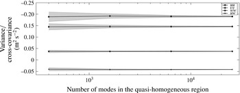
Convergence of second-order statistics with numbers of random Fourier–Gabor modes being used to enrich a single quasi-homogeneous region located at
 $z=5~\text{m}$
for PBL idealization 2 (see § 5). The shaded region indicates the standard deviation (uncertainty) about the mean of the statistics computed over several independent realizations.

2.5 Compressed representation of the subfilter scales
The random sampling of the Fourier–Gabor modes on shells with logarithmically spaced shells leads to substantial reduction in degrees of freedom (for evolution equations (2.20)–(2.22)). Logarithmic sampling avoids excessive sampling of high wavenumbers which is implied by linearly spaced sampling. Low wavenumber biased sampling has been used previously for numerical solutions to analytical theories of turbulence such as direct interaction approximation (DIA) (see Kraichnan Reference Kraichnan1964), and also in other classical applications of kinematic simulations (Fung et al.
Reference Fung, Hunt, Malik and Perkins1992) for homogeneous isotropic turbulence. Since the second-order turbulence statistics are inherently dominated by large scales (due to power-law decay of the energy spectrum), logarithmic sampling provides the ability to construct turbulent fields with very accurate one-point and two-point correlations (second-order spectra) using a very small number of spectral modes. Furthermore, these three-dimensional modes are randomly sampled, which results in fields that are essentially non-periodic in physical space. Figure 3 shows the modes that are generated as part of the enrichment in a particular quasi-homogeneous region located at
 $z=5$
in the PBL idealization 2 (see § 5) where a coarse LES is enriched with high wavenumber content synthesized using KS. In this PBL idealization, the total number of equivalent wavenumbers needed if the LES (of an equivalent spectral resolution) was performed on a finer grid (
 $72\times 72\times 36$
grid points within quasi-homogeneous region, or
 $36\times 36\times 18$
grid points within each coarse LES cell required for an equivalent spectral resolution) is approximately
 $4.5\times 10^{9}$
. A total of 6400 Fourier–Gabor modes within each quasi-homogeneous region (shown in figure 3) are sufficient to obtain statistical convergence of second-order statistics. Therefore, if the coarse LES is performed on a
 $n_{x}\times n_{y}\times n_{z}$
grid, the KS enriched LES has a total of
 $n_{x}n_{y}n_{z}+(n_{x}n_{y}n_{z}/8)6400$
degrees of freedom, whereas an equivalent high resolution LES would require
 $n_{x}n_{y}n_{z}(36\times 36\times 18)$
degrees of freedom. This corresponds to reduction in degrees of freedom (compression) of approximately 96.5 %. However, a random sampling results in uncertainty in the predicted second-order statistics. This uncertainty decays to zero, as the number of randomly sampled wavenumbers increases. This convergence is shown in figure 4. For all the simulations used in this paper a total of 6400 random modes (64 shells with logarithmically spaced radii subsequently are strained using RDT) is used. Since most of the energy is in the largest scales (smallest wavenumber) the logarithmic sampling results in statistical convergence of the second-order correlations, using a very small number of modes which is also shown in figure 4. It is also evident in figure 3 that the use of RDT along with Mann’s lifetime model generates initial conditions where the anisotropy is very strong at large scales (low wavenumber), and weak at high wavenumbers which is consistent with observations.
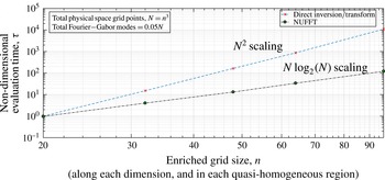
Scaling of computational time for transform from the Fourier–Gabor space to physical space on a three-dimensional Cartesian grid.

Finally, it is important to mention that since the sampled wavenumbers are no longer uniformly spaced, it is not possible to use the standard fast Fourier transform (FFT) algorithms and a direct evaluation is very expensive. However, it is possible to compute the inverse transform up to a prescribed precision using the NUFFT algorithm developed by Greengard & Lee (Reference Greengard and Lee2004) and Dutt & Rokhlin (Reference Dutt and Rokhlin1993). For problems with large compression of wavenumbers, this fast Gaussian gridding algorithm has a computational cost that is essentially equivalent to a Fourier transform on a twice oversampled grid, assuming a precision of approximately 1E-9 which is sufficient for the application discussed in this paper. Figure 5 shows the scaling of computational time in evaluating the transform using both the NUFFT algorithm and the direct inversion. In this scaling study, isotropic turbulence is generated using the KS over a series of physical space grids with increasing resolution. The number of Fourier–Gabor modes used for each grid is taken to be 5 % of the total number of grid points, thereby implying a 95 % compression in degrees of freedom. The importance of NUFFT is particularly evident for the case with
 $64^{3}$
grid (closest resemblance to the enrichment used in PBL idealization 2 and channel flow at
 $Re_{\unicode[STIX]{x1D70F}}=1000$
), where the speed up due to use of NUFFT is greater than a factor of 50.
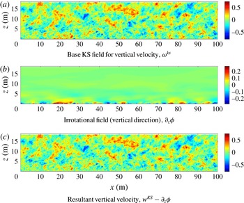
Contours of subfilter
 $w$
-velocity on the
 $x$
–
 $z$
plane that illustrate the superposition methodology used to obtain the desired no-penetration boundary condition for PBL idealization 2.

2.6 Kinematic blocking by the ground and no-penetration boundary condition
Since the Fourier–Gabor formulation cannot satisfy the no-penetration boundary condition (BC) at the ground, an additional correction to the base KS field is needed so that kinematic blocking effect felt by the subfilter eddies is correctly modelled by the enriching algorithm. Due to the high Reynolds number nature of the PBL, it is reasonable to ignore the viscous effects, and as such the no-penetration BC can be satisfied by superposing an irrotational field on the KS field synthesized using the Fourier–Gabor modes (see Lee & Hunt Reference Lee and Hunt1991; Mann Reference Mann1994). The resultant field with the correct BCs can thus be constructed as
 $$\begin{eqnarray}u_{i}(x,y,z,t)=u_{i}^{KS}(x,y,z,t)-\unicode[STIX]{x2202}_{i}\unicode[STIX]{x1D719}(x,y,z,t),\end{eqnarray}$$
where the irrotational field,
 $\unicode[STIX]{x2202}_{i}\unicode[STIX]{x1D719}$
satisfies the Laplace equation with inhomogeneous BCs
 $$\begin{eqnarray}\unicode[STIX]{x1D6FB}^{2}\unicode[STIX]{x1D719}=0,\quad \unicode[STIX]{x2202}_{z}\unicode[STIX]{x1D719}(x,y,z=0,t)=w^{KS}(x,y,z=0,t),\quad \unicode[STIX]{x2202}_{z}\unicode[STIX]{x1D719}(x,y,z\rightarrow \infty ,t)=0.\end{eqnarray}$$
The Laplace equation comes from requiring that the irrotational field,
 $\unicode[STIX]{x1D735}\unicode[STIX]{x1D719}$
satisfy the divergence free condition that is already satisfied by the KS field. Since the domain being considered for PBL idealization 2 is periodic in
 $x$
and
 $y$
directions, the solution to (2.31) can be written in terms of the planar (
 $x{-}y$
) Fourier transform of
 $\unicode[STIX]{x1D719}$
and
 $w^{KS}$
as
 $$\begin{eqnarray}\hat{\unicode[STIX]{x1D719}}(k_{x},k_{y},z)=\frac{-{\hat{w}}^{KS}(k_{x},k_{y},z=0)}{k_{2d}}\text{e}^{-k_{2d}z},\end{eqnarray}$$
where
 $k_{2d}=\sqrt{k_{x}^{2}+k_{y}^{2}}$
. This superposition procedure also generates an increment in the magnitude of the horizontal velocity components (
 $u$
and
 $v$
) which is referred to as the splatting effect by Lee & Hunt (Reference Lee and Hunt1991). Figure 6(a–c) illustrate this superposition procedure for the PBL idealization where a coarse LES is enriched using KS which generates the subfilter turbulence.
It is now possible to introduce the three problems evaluated to demonstrate the viability of the algorithm for high Reynolds number flows.
-
(i) PBL idealization 1: homogeneous mean shear. In this three-scale idealization, the surface layer is assumed to possess weak inhomogeneity thereby allowing all the scales to be described entirely using Fourier–Gabor modes. The largest scales (scale 1) are assumed to stay frozen and simply advected using Taylor’s hypothesis at a constant bulk velocity, whereas scales 2 and 3 are evolved using the equations discussed in § 2.3.
-
(ii) Channel flow at
$Re_{\unicode[STIX]{x1D70F}}=1000$
. In this two-scale simulation, the largest scales are obtained from a filtered version of a direct numerical simulation. The filtered version of the DNS serves as a surrogate for an LES and the smaller scales are enriched using the KS. -
(iii) PBL idealization 2: stratified TBL with Coriolis and geostrophic forcing. In this two-scale simulation, the largest scales come from a filtered version of a high resolution large eddy simulation, thereby preserving the inhomogeneities inherent in the problem. The smaller scales (scale 2) are enriched using the KS.

3 PBL idealization 1: homogeneous mean shear
3.1 Problem description and assumptions
A popular idealization for the PBL often used in literature is that of an infinite Reynolds number boundary layer (see Porté-Agel, Meneveau & Parlange Reference Porté-Agel, Meneveau and Parlange2000; Bou-Zeid, Meneveau & Parlange Reference Bou-Zeid, Meneveau and Parlange2005; Stevens, Wilczek & Meneveau Reference Stevens, Wilczek and Meneveau2014), where a constant favourable pressure gradient (
 $u_{\star }^{2}/H$
) is used to drive the flow in a half-channel of height
 $H$
with an implied surface shear stress
 $u_{\star }^{2}$
. The use of wall model at the surface along with the blocking effect due to no-penetration BC at the surface causes inhomogeneity in the vertical direction, with the turbulent shear stress decreasing linearly as a function of height,
 $z$
. The PBL idealization 1 discussed in this section will consider the flow features along the
 $x{-}y$
plane located at height,
 $z=0.154H$
.
The principal assumption in this idealization is the following: within a small layer
 $0.154H-L_{z}<z<0.154H+L_{z}$
, we assume that the flow is homogeneous with a constant mean shear given by the value
 $\text{d}\langle u\rangle /\text{d}z(z=0.154H)$
. While such an assumption of weak homogeneity is only valid for small values of
 $L_{z}$
, it is a reasonable assumption for engineering applications such as wind turbines or pollutant plumes which have length scales of the same order as
 $L_{z}$
. The main advantage of this weak homogeneity assumption is that we can express the entire fluctuating velocity field (including the largest scales) using Fourier modes. This assumption of homogeneous turbulence requires the mean flow to follow,
 $$\begin{eqnarray}\frac{\unicode[STIX]{x2202}\langle u_{i}\rangle }{\unicode[STIX]{x2202}x_{j}}=\text{const.},\quad \frac{\unicode[STIX]{x2202}\langle \unicode[STIX]{x1D703}\rangle }{\unicode[STIX]{x2202}x_{j}}=\text{const.},\end{eqnarray}$$
which subsequently allows us to evaluate the velocity fields in scale 1 using randomly sampled Fourier modes. In this idealization, we further assume that scale 1 remains frozen and is simply advected in accordance to Taylor’s hypothesis. Using these two assumptions, the velocity field in scale 1 can be written as
 $$\begin{eqnarray}\boldsymbol{U}^{(1)}(\boldsymbol{x},t)=\mathop{\sum }_{m}\boldsymbol{a}_{m}\exp [\text{i}\boldsymbol{k}_{m}\boldsymbol{\cdot }(\boldsymbol{x}-\boldsymbol{U}_{0}t)]\end{eqnarray}$$
and
 $$\begin{eqnarray}\unicode[STIX]{x1D703}^{(1)}(\boldsymbol{x},t)=\mathop{\sum }_{m}\hat{\unicode[STIX]{x1D703}}_{m}\exp [\text{i}\boldsymbol{k}_{m}\boldsymbol{\cdot }(\boldsymbol{x}-\boldsymbol{U}_{0}t)],\end{eqnarray}$$
where
 $\boldsymbol{U}_{0}$
is a constant, bulk velocity, and
 $\boldsymbol{x}$
is a location anywhere in the full domain,
 $\unicode[STIX]{x1D6FA}(\mathbb{R}^{3})$
. While the assumption of vertical homogeneity made in PBL idealization 1 appears to be grossly inaccurate, it is plausible in engineering applications involving objects (such as finite size wind farms) where the decorrelation time of the largest scales is much larger than the advection time through the finite length domain.
A total of three scales are used in the kinematic simulation: scale 1 (frozen and advected) comprising of
 $kL<0.6$
, scale 2 (swept and strained by scale 1) comprising of
 $0.6<kL<6$
and scale 3 (swept and strained by scales 1 and 2) comprising of
 $kL>6$
. The length scale
 $L$
and the value of the shearing constant,
 $c_{\unicode[STIX]{x1D70F}}$
needed for initialization are taken to be
 $0.075H$
and 2.5 respectively. The value of
 $c_{\unicode[STIX]{x1D70F}}$
is determined using a procedure very similar to the one described in appendix A. Since this problem corresponds to a constant pressure driven turbulent boundary layer (TBL) at very high Reynolds number, it is easy to observe that
 $\langle \tilde{u} \tilde{w}\rangle (z)+\unicode[STIX]{x1D70F}_{xz}^{SGS}(z)=u_{\star }^{2}(1-z/H)$
. This relation replaces (B 2) and (B 4) (in appendix B) and subsequently the value of
 $c_{\unicode[STIX]{x1D70F}}$
can be evaluated at
 $z=0.154H$
. Therefore, the value of cross-correlation
 $uw$
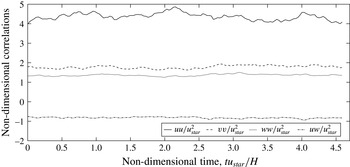
computed using KS is expected to match the theoretical value. Finally, note that since the results discussed in this paper do not involve simulation over very long times, this quenching and replacement procedure discussed earlier was not required, since stationarity of the statistics was not violated as is seen in figure 7.
Time history of the second-order statistics for the KS in PBL idealization 1.

3.2 Results and discussion
Table 2 reports the single-point correlation values obtained using the KS and LES performed using two different methodologies. The first set of LES results are taken from Wilczek, Stevens & Meneveau (Reference Wilczek, Stevens and Meneveau2015) who have performed LES on a
 $1024\times 512\times 256$
mesh using a code that uses the Lagrangian-averaged dynamic Smagorinsky model (see Bou-Zeid et al.
Reference Bou-Zeid, Meneveau and Parlange2005) for a roughness length scale of
 $z_{0}=10^{-4}H$
. The second LES reported in table 2, which is performed on a coarser mesh, uses the code described in appendix A where the subgrid closure is provided by the Sigma model (see Nicoud et al.
Reference Nicoud, Toda, Cabrit, Bose and Lee2011). The domain size considered in this LES is
 $4\unicode[STIX]{x03C0}H\times 2\unicode[STIX]{x03C0}H\times H$
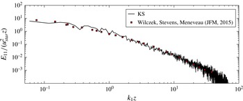
. The wall model used by both the LES methodologies is identical and is described in Bou-Zeid et al. (Reference Bou-Zeid, Meneveau and Parlange2005). The values for second-order correlations reported in table 2 verify that the anisotropy in the turbulence synthesized using the KS is reasonably accurate. Figure 8 shows further evidence for this claim by comparing the autospectra (two-point correlation) of the longitudinal velocity (
 $u$
) between KS and the high resolution LES reported in Wilczek et al. (Reference Wilczek, Stevens and Meneveau2015).
Comparison of second-order one-point correlations (at
 $z=0.154H$
) of the KS synthesized turbulence compared with LES results. The exact value for the cross-correlation is expected to asymptote to
 $-0.846$
.

Comparison of autospectra of longitudinal fluctuations between the KS and the LES by Wilczek et al. (Reference Wilczek, Stevens and Meneveau2015), taken at
 $z/H=0.154$
.

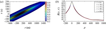
(a) Space–time correlation,
 $R(r,\unicode[STIX]{x1D70F})$
contours at the
 $z/H=0.154$
plane obtained using the KS. (b) Space–time correlations
 $R(r,\unicode[STIX]{x1D70F})$
for different time separations
 $\unicode[STIX]{x1D70F}$
at
 $z/H=0.154$
versus the separation
 $r_{E}=\sqrt{(r-U\unicode[STIX]{x1D70F})^{2}+V^{2}\unicode[STIX]{x1D70F}^{2}}$
as defined by elliptic model derived by He & Zhang (Reference He and Zhang2006).

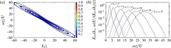
Normalized
 $k{-}\unicode[STIX]{x1D714}$
spectrum with contours spaced logarithmically are shown in (a). Panel (b) shows slices along lines of constant wavenumber
 $k_{1}$
with varying
 $\unicode[STIX]{x1D714}$
. The coloured lines correspond to LES data (taken from Wilczek et al.
Reference Wilczek, Stevens and Meneveau2015) whereas the black lines correspond to the KS.

The temporal accuracy of the KS fields can be evaluated by studying their space–time correlations. As shown in figure 9, the space–time correlation contours do form closed ellipses with eccentricities that are consistent with those predicted by the model given by He & Zhang (Reference He and Zhang2006). The elongated contours show that the turbulence generated using the KS is primarily advected by the bulk velocity; however, it decorrelates in time. Furthermore, it shows that eddies of smaller size (higher wavenumbers) decorrelate faster than the eddies of larger size. In this simulation, the scale with the smallest wavenumber is frozen and hence the space–time correlations do not entirely go to zero.
To enable further comparison of the space–time properties of the velocity fields synthesized using the KS, figure 10 shows the
 $k{-}\unicode[STIX]{x1D714}$
spectrum along with the results reported in Wilczek et al. (Reference Wilczek, Stevens and Meneveau2015). The preferential direction corresponds to the Doppler shift due to mean velocity whereas the Doppler broadening corresponds to the effect of turbulence decorrelation due to inter-scale interactions. The comparison with LES suggests that the overall broadening of the spectrum is correctly predicted by the KS. We acknowledge some discrepancies in low frequency, high wavenumber range of the
 $k{-}\unicode[STIX]{x1D714}$
spectrum (see the vertical dotted lines in figure 10
b) where the LES results seem to suggest strong negative skewness causing substantial deviation from the largely Gaussian spectrum predicted by the KS model. However, we note that the deviations from Gaussian behaviour (leptokurtic) observed at lower wavenumbers is quite well predicted by the KS. The negative skewness observed at high wavenumbers in the LES results suggests physics that is not modelled (or modelled inaccurately), and will be investigated further in future work. Possible sources of error include inaccurate/incomplete modelling of the nonlinear interactions via the spectral viscosity, and the use of large scales that are frozen. Note that in order to compute the
 $k{-}\unicode[STIX]{x1D714}$
spectrum using the KS fields, we need to perform windowing in both space (
 $x_{1}$
-coordinate) and time (
 $t$
) since the KS-generated fields are non-periodic in physical space.
Finally, it is important to acknowledge that while the use of RDT-like closure to model straining of small scales by the large-scale results in realistic anisotropy of the synthesized fields, the higher-order statistics responsible for phenomena such as intermittency are not quantitatively accurate. For example, the skewness of the
 $u$
- and
 $w$
-velocity fields (non-dimensionalized using
 $u_{\star }$
) synthesized using KS are approximately
 $0.07$
and
 $-0.06$
respectively, whereas those by Stevens et al. (Reference Stevens, Wilczek and Meneveau2014) in their LES simulations are approximately
 $0.2$
and
 $-0.25$
at
 $z/H=0.154$
. Therefore, while the use of RDT results in qualitatively correct skewness (for the three primitive variables), the magnitudes are not accurate which is primarily due to the nonlinear viscosity closure used for nonlinear interactions at small scales. Other closures such as those based on random forcing models, can potentially address this drawback of the KS enrichment approach. We further acknowledge that at Reynolds numbers of relevance to PBL turbulence, higher moments involving velocity gradients are unlikely to be correctly predicted by either conventional LES or enriched LES due to their inherent high wavenumber (dissipation range) bias.
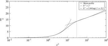
Mean velocity profile for channel at
 $Re_{\unicode[STIX]{x1D70F}}=1000$
. The vertical line corresponds to
 $z^{+}=30$
height, above which the log-layer can be assumed to be valid.

4 Finite Reynolds number case: channel flow at
$Re_{\unicode[STIX]{x1D70F}}=1000$

4.1 Problem description and comparison methodology
The finite Reynolds number channel flow is a canonical turbulent boundary layer flow that has traditionally served as a validation problem for most large eddy simulations of wall-bounded flows. Here we consider the channel flow DNS at a friction Reynolds number,
 $Re_{\unicode[STIX]{x1D70F}}=1000$
, performed using the peta-scale channel flow code developed by Lee, Malaya & Moser (Reference Lee, Malaya and Moser2013). The simulated domain size is
 $8\unicode[STIX]{x03C0}H\times 3\unicode[STIX]{x03C0}H\times 2H$
(
 $H$
is the channel half-width) and the full DNS flow fields were accessed via the Johns Hopkins Turbulence Database (see Perlman et al. (Reference Perlman, Burns, Li and Meneveau2007), Li et al. (Reference Li, Perlman, Wan, Yang, Meneveau, Burns, Chen, Szalay and Eyink2008), Graham et al. (Reference Graham, Kanov, Yang, Lee, Malaya, Lalescu, Burns, Eyink, Szalay, Moser and Meneveau2016) for further details of the simulation and the database). Furthermore, note that in order to maintain consistency in coordinate systems throughout this paper, the wall-normal direction is assumed to be
 $z$
, as opposed to
 $y$
which is the case in original DNS simulation, and in most channel flow simulations.
Figure 11 shows the mean velocity profile for the longitudinal velocity,
 $u$
, in wall units (
 $z^{+}=zu^{\star }/\unicode[STIX]{x1D708}$
,
 $U^{+}=u/u^{\star }$
). The viscous and buffer layers extend up to a wall-normal distance of approximately
 $30$
(in
 $+$
units), and influence of the viscous no-slip wall persists in this region. The velocity field fluctuations in
 $z^{+}<20$
is largely two-component, and hence cannot be synthesized using KS due to the RDT-like linearization that is implicit in its formulation. However, for
 $z^{+}>30$
, the self-similarity of the log-law is quite evident from figure 11 and can serve as a reasonable test case for KS enriched LES. It is important to note that for
 $Re_{\unicode[STIX]{x1D70F}}=1000$
, the
 $z^{+}<30$
corresponds to the bottom 3 % of the channel half-width, and hence KS enrichment in
 $z^{+}>30$
still spans a substantial portion of the simulated domain.
The results shown in the remainder of this section correspond to the following three simulation cases.
-
(i) Baseline DNS: channel flow DNS dataset from Johns Hopkins Turbulence Database. Simulation performed on a
$2048\times 1536\times 512$
numerical grid. -
(ii) LES (filtered DNS): this corresponds to filtered fields from the baseline DNS used as a surrogate for LES performed on a
$128\times 96\times 128$
numerical grid. -
(iii) Enriched LES: this corresponds to the superposition of the subfilter KS field onto the LES fields. This is accomplished by assigning each adjacent set of
$2\times 2\times 2$
filtered LES cells to a single quasi-homogeneous region. Each quasi-homogeneous region is enriched with subfilter fields synthesized using KS with
$6400$
Fourier–Gabor modes, and can be resolved on a
$36\times 72\times 16$
grid. This implies that the entire enriched LES is resolved on to a
$2304\times 1728\times 1024$
grid.




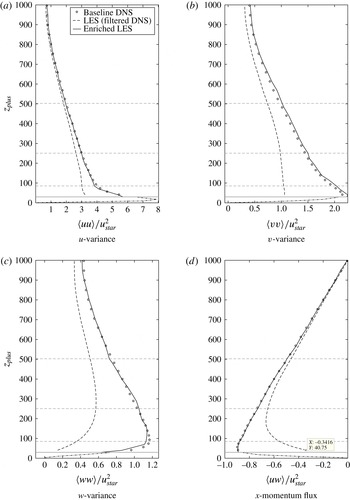
Mean profiles of second-order (single-point) correlations.

4.2 Results and discussion
The vertical profiles of second-order correlations are shown in figure 12. The figures show that the KS enrichment accounts for substantial portion of the turbulent kinetic energy close to wall (
 ${\approx}50\,\%$
at
 $z^{+}=30$
), which reduces with distance from the wall. Since the integral length scale of turbulence increases with distance from the wall, the LES simulation is capable to capturing the bulk of the single-point correlations and the relevance of the enriching KS fields is decreased. Since the KS enriched fields match the local turbulent kinetic energy production rate with the DNS (see discussion in appendix B), the Reynolds stress of the KS enriched LES matches that of the DNS exactly. The resulting variance for the longitudinal fluctuations,
 $u$
also appear to match the DNS fairly accurately through the bulk of the turbulent boundary layer. The slight over-prediction of the spanwise velocity (
 $v$
) variance is evident from figure 12(b), with the maximum deviation occurring close to the wall. It is also interesting to note that at this same location, the variances of both the vertical (
 $w$
) and longitudinal (
 $u$
) velocity fluctuations are under-predicted. This also suggests that while the small-scale structures enriched by KS near the wall are substantially anisotropic (large
 $\langle uw\rangle$
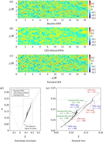
), they tend to be more oblate than those obtained using DNS. This is further confirmed by studying the anisotropy invariants in the Lumley triangle shown in figure 16(d,e). This drawback appears to be a consequence of the RDT straining during initialization which over-predicts the transfer of energy from the
 $w$
fluctuations to
 $v$
fluctuations and under-predicts the transfer of energy from
 $w$
fluctuations to
 $u$
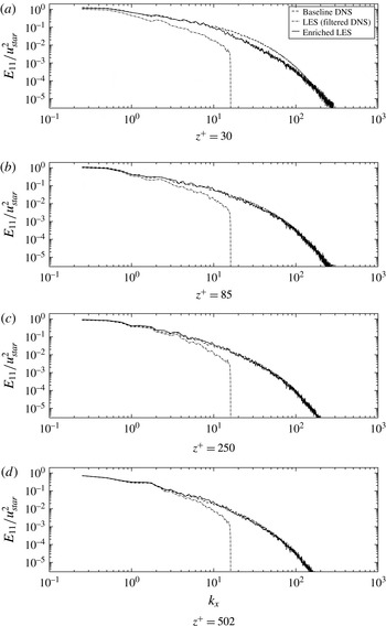
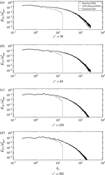
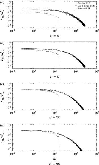
fluctuations. However the discrepancies appear to largely disappear with increasing distance from the wall, since the small scales enriched by the KS become increasingly isotropic. The autospectra for the three velocity coordinates are also shown in figures 13 through 15 at four different locations with varying distance from the wall. The spectra show that the finite Reynolds number modification made to the pre-initialization isotropic turbulence energy spectrum results in fairly accurate prediction of the dissipation range for the highly anisotropic wall turbulence. The spectra also show that the KS enrichment provides a consistent extrapolation for LES spectra, which is confirmed via the comparisons with DNS.
Autospectra of
 $u$
-velocity fluctuations taken at varying
 $z$
-locations (heights).

Autospectra of
 $v$
-velocity fluctuations taken at varying
 $z$
-locations (heights).

Autospectra of
 $w$
-velocity fluctuations taken at varying
 $z$
-locations (heights).

Panels (a–c) show contours of spanwise velocity,
 $v$
, on the
 $x{-}y$
plane (subdomain) taken at
 $z^{+}=85$
. Panels (d,e) show the anisotropy invariants
 $(\unicode[STIX]{x1D709},\unicode[STIX]{x1D702})$
plotted on the Lumley triangle for
 $z^{+}>30$
. Note that the LES results were upsampled on to the DNS grid before computing the anisotropy invariants using linear interpolation.

5 PBL idealization 2: stably stratified turbulent boundary layer with Coriolis and geostrophic forcing
5.1 Problem description and comparison methodology
The assumption of weak homogeneity used in idealization 1 is not valid at large vertical scales, especially at scales comparable to the size of the surface layer. Furthermore, realistic PBL turbulence experiences effects of stratification. Inhomogeneity in the vertical direction is also caused by the Coriolis force (which results in veer in the wind direction), kinematic blocking from the ground and scalar fluxes (which cause inhomogeneity close to the ground where production dominates transport), and due to the presence of a capping inversion which limits the height of the boundary layer. In order to investigate the performance of the KS enrichment approach when all these interactions are prevalent, the stably stratified polar atmospheric boundary layer simulated in the Global Energy and Water Cycle Experiment Atmospheric Boundary Layer Study (GABLS) LES (see Beare et al. Reference Beare, Macvean, Holtslag, Cuxart, Esau, Golaz, Jimenez, Khairoutdinov, Kosovic and Lewellen2006) is used in this idealization. The details of the LES code used are described in appendix A. The recent paper by Sullivan et al. (Reference Sullivan, Weil, Patton, Jonker and Mironov2016) presents detailed discussion of the physics observed and the simulation challenges, for the problem being considered in this idealization.
All results shown in this section come from three datasets and are averages taken between hour 7 and hour 8 of the simulation:
-
(i) Baseline LES: this corresponds to a full LES conducted on a
$512\times 512\times 512$
grid corresponding to a domain of
$400~\text{m}\times 400~\text{m}\times 400~\text{m}$
. The details of the numerics, boundary and initial conditions and the subgrid model used are provided in appendix A. -
(ii) Filtered LES: this corresponds to the filtered representation of the baseline LES. To obtain these data, the fields from the baseline LES are filtered (using the filters shown in figure 2) onto a
$40\times 40\times 128$
grid corresponding to the same domain used in the baseline LES. In order to create contour plots shown in this section, this filtered field is subsequently upsampled back onto the grid used by the baseline LES using linear interpolation, which is consistent with the quasi-homogeneous assumption in (2.16). -
(iii) Enriched LES: this corresponds to the superposition of the subfilter KS field onto the filtered LES. This is accomplished by assigning each adjacent set of
$2\times 2\times 2$
filtered LES cells to a single quasi-homogeneous region. Each quasi-homogeneous region is enriched with subfilter fields synthesized using KS (with 6400 Fourier–Gabor modes) and can be resolved on a
$72\times 72\times 36$
grid. This implies that the entire enriched LES is resolved on to a
$1440\times 1440\times 2304$
grid which corresponds to the same domain as the one used in the baseline LES.





For this idealization, the KS enrichment algorithm is appraised using the second-order spatial correlations and spectra; we do not present the results for temporal evolution (which was done for idealization 1) of the enriched LES. This topic will be addressed in a subsequent paper where an a posteriori approach is used to obtain the coarse LES (as opposed to using a higher resolution LES filtered onto a coarse grid) thereby allowing consistent temporal filtering.
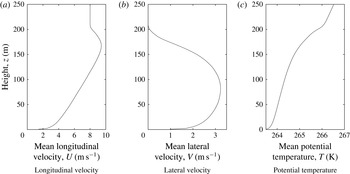
Mean profiles of the primitive variables averaged in the horizontal plane and in time between hour 7 and hour 8 of the simulation. The supergeostrophic jet appears at a height of approximately 170 m and the height of the boundary layer is approximately 200 m.

Figure 17 shows the mean vertical profiles for the longitudinal velocity
 $U$
, the lateral velocity
 $V$
and the potential temperature,
 $T$
. The height of the boundary layer, defined as the location where
 $(\langle uw\rangle ^{2}+\langle vw\rangle ^{2})^{1/2}$
reaches a value lower than 5 % of its surface value (
 $u_{\star }^{2}$
), is evaluated as approximately 190 m which is in agreement with results in Beare et al. (Reference Beare, Macvean, Holtslag, Cuxart, Esau, Golaz, Jimenez, Khairoutdinov, Kosovic and Lewellen2006) (170–200 m).
5.2 Input parameters
In order to initialize the KS enrichment, we need to specify certain input parameters discussed previously in § 2.4. The initial spectrum used to synthesize the pre-sheared isotropic turbulence requires specification of the dissipation rates,
 $\unicode[STIX]{x1D700}$
and
 $\unicode[STIX]{x1D700}_{\unicode[STIX]{x1D703}}$
, which in turn require estimates for
 $\langle uw\rangle$
,
 $\langle vw\rangle$
and
 $\langle w\unicode[STIX]{x1D703}\rangle$
. The mean gradients
 $\text{d}U/\text{d}z$
,
 $\text{d}V/\text{d}z$
and
 $\text{d}\unicode[STIX]{x1D6E9}/\text{d}z$
are computed from the baseline LES results shown in figure 17. The fundamental assumption made here is that the mean profiles can be well predicted by an LES performed on a coarse mesh. While there is strong evidence that suggests that this assumption is not strictly true (see Sullivan et al.
Reference Sullivan, Weil, Patton, Jonker and Mironov2016), it is most certainly true in this study since the coarse LES is emulated by filtering the baseline LES. As is shown in appendix B, once the mean gradients are known, the fluxes
 $\langle uw\rangle$
,
 $\langle vw\rangle$
and
 $\langle w\unicode[STIX]{x1D703}\rangle$
can be estimated using their respective surface values, which are provided by the wall model used in the LES. For the purpose of this study, these surface values are taken directly as the values computed using the baseline LES. The baseline LES predicts a
 $u_{\star }=0.245~\text{m}~\text{s}^{-1}$
and
 $T_{\star }=-0.00982~\text{Km}~\text{s}^{-1}$
which are in close agreement with the recent calculations of Sullivan et al. (Reference Sullivan, Weil, Patton, Jonker and Mironov2016) (
 $u_{\star }=0.255~\text{m}~\text{s}^{-1}$
,
 $T_{\star }=-0.00963~\text{Km}~\text{s}^{-1}$
) on a
 $1024^{3}$
mesh.
Profile of the shearing constant,
 $c_{\unicode[STIX]{x1D70F}}$
determined for the PBL idealization 2 in panel (a). The profile of the integral length scale used to synthesize the pre-initialization isotropic turbulence is shown in panel (b). This profile is directly computed using the coarse (in this case filtered) LES. The horizontal dashed lines correspond to the edges of the quasi-homogeneous layers.

The two other input parameters that need to be specified are the shearing constant,
 $c_{\unicode[STIX]{x1D70F}}$
and the representative length scale,
 $L$
used to generate the pre-sheared isotropic turbulence. The length scale,
 $L$
is computed as a function of
 $z$
, using the filtered LES data
 $$\begin{eqnarray}L(z)=c_{L}\sqrt{L_{x}^{LES}(z)L_{y}^{LES}(z)}.\end{eqnarray}$$
The constant
 $c_{L}$
is taken to be 0.6. The longitudinal and lateral length scales,
 $L_{x}$
and
 $L_{y}$
are computed at each
 $z$
location by computing autocorrelation of the longitudinal velocity
 $u$
, in
 $x$
and
 $y$
directions. Following the specification of
 $L$
, the shearing constant
 $c_{\unicode[STIX]{x1D70F}}$
can be directly computed by minimizing a least square error involving cross-correlations
 $\langle uw\rangle$
,
 $\langle vw\rangle$
and
 $\langle w\unicode[STIX]{x1D703}\rangle$
, and is discussed in appendix B. The profiles of the two input parameters,
 $c_{\unicode[STIX]{x1D70F}}$
and
 $L$
are shown in figure 18.
Finally, note that since the flow is homogeneous in
 $x$
- and
 $y$
-directions, the input parameters vary only in the
 $z$
-directions, which leads to the quasi-homogeneous layers shown using the dashed horizontal lines. Between each quasi-homogeneous layer, the state of the KS enriched turbulence is fundamentally different (in terms of second-order statistics). As was mentioned in the problem description, since a quasi-homogeneous region is taken to be the subdomain comprising of
 $2\times 2\times 2$
filtered LES cells, we have a total of 64 quasi-homogeneous layers (and
 $20\times 20\times 64$
quasi-homogeneous subdomains) in the entire problem domain. Since the boundary layer turbulence is active only in the bottom half of the domain due to the strong inversion layer, all the results shown in the subsequent section are only shown through a height of 200 m.
Other implementation details, such as the blending functions used to obtain at least
 $\mathbb{C}^{0}$
continuity in the fields at the edges of the quasi-homogeneous regions, are discussed in appendix C. The velocity fields synthesized in two vertically adjacent quasi-homogeneous regions are essentially independent, and hence the transport in the vertical direction between two adjacent layers is not captured. However, the enriched fields in horizontally (
 $x$
- and
 $y$
-) adjacent quasi-homogeneous regions cannot be statistically independent since the dominant transport occurs in the horizontal plane (since
 $\overline{U}(z)\neq 0$
,
 $\overline{V}(z)\neq 0$
). Hence the Fourier–Gabor modes in horizontally adjacent regions are constructed as modes from a single set of synthesized modes for each
 $z$
-layer, using the shift theorem. This ensures that the space–time correlation along
 $x$
- and
 $y$
-directions is correct. Two vertically adjacent quasi-homogeneous regions are essentially independent due to inhomogeneity present in this direction. This requires the use trigonometric blending functions in the vertical directions in order to obtain a smooth transition in second-order correlations within the overlap region. Further details regarding this blending procedure, along with some comments regarding the resulting divergence error within the overlap region, are provided in appendix C.
Mean profiles of second-order (single-point) correlations (a–h). Panel (i) shows the flux Richardson number.

Contours of longitudinal velocity
 $u$
on the
 $x{-}y$
plane taken at
 $z=6~\text{m}$
.

5.3 Results and discussion
The vertical profiles of second-order correlations are shown in figure 19. The horizontal dashed lines correspond to the two vertical locations where further details in terms of spectra are analysed. The single-point cross-correlations (figure 19
a–c) obtained for the enriched LES are in excellent agreement with the baseline LES. Note that in these three panels, the cross-correlations for the LES have contributions from both the resolved and the modelled subgrid components. The justification for this is provided in appendix B. Note that these comparisons of the cross-correlations are expected to be good since the shearing constant,
 $c_{\unicode[STIX]{x1D70F}}$
is computed by minimizing the least square error in a term involving the three cross-correlations. The variances shown in figure 19(d–f) also show excellent agreement with the LES results. The deviations are primarily limited in the top region of the boundary layer, around and above the location of the supergeostrophic jet and the inversion layer. This trend is also visible in the variances shown in figure 19(d–f), where the
 $w$
-fluctuations seem to be over-predicted near the inversion layer. It is also evident that while the turbulent kinetic energy is well predicted throughout the stable boundary layer, the temperature variances are over-estimated by the enrichment process near the location of the geostrophic jet, where the influence of the inversion is substantial. This suggests that near the top of the boundary layer, the complex dynamics associated with interactions with the high stratification in the inversion layer is not fully captured by RDT-like linear theory, which tends to generate subfilter turbulence that is slightly more isotropic (higher
 $ww$
and lower
 $vv$
) than the baseline LES predicts for the smaller scales. Further insight into this region can be provided by studying the behaviour of the flux Richardson number (defined as
 $Ri_{f}=(g/T_{0}\langle w\unicode[STIX]{x1D703}\rangle )/(\langle uw\rangle \,\text{d}U/\text{d}z+\langle vw\rangle \,\text{d}V/\text{d}z)$
and shown in figure 19(i)) which tends to sharply diverge (to a large positive value) as the momentum fluxes approach zero much faster than the temperature flux which reaches a value of zero at the top of the boundary layer as an approximately linear function of
 $z$
(see discussion at the end of appendix B). This combination of high buoyancy destruction and relatively large length scale (shown in figure 22
b) implying that LES resolves most of the energetic scales, results in KS turbulence that is largely isotropic. This is also validated by the observation that while
 $ww$
is slightly over-predicted, and
 $\unicode[STIX]{x1D703}\unicode[STIX]{x1D703}$
is over-predicted, the cross-correlation,
 $w\unicode[STIX]{x1D703}$
is still slightly under-predicted.
 $x$
-direction spectra of
 $u$
-fluctuations taken at a height
 $z=6~\text{m}$
.

Contours of lateral velocity
 $v$
on the
 $x{-}y$
plane taken at
 $z=6~\text{m}$
.

 $x$
-direction spectra of
 $v$
-fluctuations taken at a height
 $z=6~\text{m}$
.

Contours of potential temperature
 $\unicode[STIX]{x1D703}$
on the
 $x{-}y$
plane taken at
 $z=6~\text{m}$
.

 $x$
-direction spectra of
 $\unicode[STIX]{x1D703}$
– fluctuations taken at a height
 $z=6~\text{m}$
.

 $x$
-direction spectra for the turbulent fields taken at
 $z=100~\text{m}$
.

The other notable discrepancy is in the over-prediction of the variances of horizontal components (
 $u$
and
 $v$
) of velocity very close to the ground. The primary cause of this discrepancy is the under-prediction of variances by the LES very close to the ground. The evidence for this claim is provided in the figures 21 and 23 which compare the autospectra of
 $u$
and
 $v$
components at a plane located at
 $z=6~\text{m}$
. The spectra from LES clearly show strong deviations (excess decay) from the
 $-5/3$
law expected for this infinite Reynolds number idealization. This excess decay at high wavenumbers is due to non-exactness of the subgrid-scale model being used. Some supporting evidence can be found in a recent paper by Abkar, Bae & Moin (Reference Abkar, Bae and Moin2016) where they have implemented the anisotropic minimum dissipation (AMD) for infinite Reynolds number, rough wall boundary layer (similar to the problem studied in PBL idealization 1), to show that their model essentially alleviates this high wavenumber decay in both velocity spectra and scalar spectra. As is shown in these figures, the enriched LES does not suffer from this high wavenumber decay and follows the expected
 $-5/3$
rule exactly in the inertial subrange. This decay is also observed to a lesser extent in figure 26 which shows the same spectra, but at a higher location (
 $z=100~\text{m}$
) in the turbulent boundary layer.
Contours of lateral velocity
 $v$
on the
 $x{-}y$
plane taken at
 $z=100~\text{m}$
.

The ratios
 $E_{21}/E_{11}$
and
 $E_{31}/E_{11}$
for the enriched LES taken at
 $z=100~\text{m}$
.

The ratios
 $E_{21}/E_{11}$
and
 $E_{31}/E_{11}$
taken at
 $z=100~\text{m}$
are shown in figure 28. The local isotropy hypothesis which implies an asymptote to a value of
 $4/3$
for the two ratios is obtained for the enriched LES. Since the PBL problem, which is assumed to have an asymptotically infinite Reynolds number, uses KS enrichment with pre-initialization isotropic turbulence obeying a
 $-5/3$
law for large
 $k$
, the local isotropy seen for high wavenumbers in enriched LES is not surprising. However, it is interesting to note that the enriched LES results show that the ratio
 $E_{21}/E_{11}$
asymptotes to
 $4/3$
at a wavenumber approximately an octave smaller than where the ratio
 $E_{31}/E_{11}$
levels off to
 $4/3$
; a prediction that is consistent with the observations reported by Kaimal (Reference Kaimal1973) for surface layer turbulence under stable stratification.
Another behaviour that is consistently observed in KS enriched fields (see figures 8, 20, 22, 25, 28) is the increased noise in the laterally (
 $y$
-direction) averaged spectra. The primary cause of this is the random sampling of wavenumbers over logarithmically spaced shells (see figure 3) which generates a substantially lower sampling of high wavenumbers relative to the uniformly spaced sampling (as is done in the baseline LES). This noise is directly related to the statistical uncertainty in single-point correlations shown in figure 4. For most practical applications, this is not expected to be an issue especially in problems requiring ensemble averaging.
Contours and correlations of exact and KS-generated subfilter scales of horizontal components of velocity at
 $z=6~\text{m}$
. The straight lines in panels (c,d) make an angle of approximately
 $17$
degrees with respect to the
 $x$
-axis, whereas those in panels (g,h) make an angle of approximately
 $62$
degrees with respect to the
 $x$
-axis.

The other interesting observation that can be made using the contour plots in figures 20 and 22 is directional bias in the orientation of the structures observed in
 $u$
- and
 $v$
-fields. This bias is direct consequence of
 $\text{d}\overline{V}/\text{d}z(z)\neq 0$
, which is turn results due to presence of the Coriolis force. Note that for the enriched scales, the direct effect of the Coriolis force is rather weak due to separation in time scales. The Rossby number defined as
 $G/(2\unicode[STIX]{x1D6FA}H)$
(
 $G$
is the geostrophic wind,
 $H$
is the height of the TBL,
 $\unicode[STIX]{x1D6FA}$
is Earth’s rotation rate) is rather high in this PBL idealization (
 $Ro\approx 275$
), and the turbulent turn over time scales decrease with increasing wavenumbers (
 $\unicode[STIX]{x1D70F}_{k}\propto k^{-1/3}$
). However, the mean gradient which manifests itself in the RDT-like straining term causes the strong orientations observed in the velocity fluctuations. The orientation of the small-scale structures is studied more closely using the two-point correlations
 $R(r_{x},r_{y})=\langle u_{i}(x+r_{x},y+r_{y})u_{i}(x,y)\rangle$
at
 $z=6~\text{m}$
. Figure 29 shows the contour plots and normalized two-point correlations (
 $R(r_{x},r_{y})/R(0,0)$
) of the subfilter
 $u$
and
 $v$
velocity components to illustrate the directional bias observed. The exact subfilter scales are computed by subtracting the filtered LES from the baseline LES. While it is easy to see that the two-point correlations of the smaller scales generated by the KS closely agree with the exact subfilter scales (which is expected since the spectra agree very well), the orientation predicted by the KS is also quite accurate for both
 $u$
and
 $v$
. The contour plots also confirm that the KS synthesized subfilter field has more fine-scale structures than the exact subfilter field (computed using LES) which experiences increased damping/decay at high wavenumbers due to the non-exact subgrid model used.
6 Conclusion
The paper outlines the development of a physics-based modelling approach to significantly increase the spatial and temporal bandwidths of PBL turbulence simulations in a cost-effective manner. The approach is based on combining an eddy resolving turbulence simulation (such as LES), albeit of limited bandwidth, with an efficient, physics-based scale enrichment scheme applied at each of the computational cells. The enrichment scheme generates a physically consistent realization of the finer-scale eddies locally which dynamically respond to the resolved larger scales and can enable statistical predictions of physical quantities with a substantially larger bandwidth. Based on the local flow information in each computational cell, the flow variables are enriched to add fine-scale subgrid fluctuations using a finite sparse mode representation. The degrees of freedom associated with the fine-scale modes evolve as ordinary differential equations in a local Lagrangian frame. The spatial transport of fine-scale modes (local advection) and scale-space transport (straining, activation/decay due to modal energy transfer, decorrelation) are treated efficiently and with reasonable accuracy.
In order to judge the viability of the simulation algorithm we investigate two idealizations of the PBL. In the first idealization, the surface layer is approximated using a uniform shear, without any temperature gradient (neutrally stratified) which makes the problem homogeneous. The high latitude stable PBL used in the GABLS1 intercomparison study (Beare et al. Reference Beare, Macvean, Holtslag, Cuxart, Esau, Golaz, Jimenez, Khairoutdinov, Kosovic and Lewellen2006) serves as the second idealization for the PBL and it further introduces the Coriolis force and stratification effects. These two idealizations demonstrate the following: (i) accurate space–time representation and evolution of the subfilter-scale dynamics, validated via comparison of second-order two-point correlations in space and time with high resolution LES, (ii) consistent extrapolation of spatial spectra (thereby extending the spectral bandwidth) of coarse grained LES (emulated by filtering high resolution LES), along with accurate prediction of enriched single-point cross-correlations and variances and (iii) substantial reduction in degrees of freedom for representation of subfilter scales by informed sampling of discrete Fourier–Gabor modes. While the synthesized fields do not predict quantitatively accurate higher-order moments, the skewness of the synthesized fields appears to be qualitatively consistent with the predictions made using fully nonlinear simulations. Furthermore, this deficiency does not appear to be of great relevance to the applications being targeted (wind turbine fatigue loading, power fluctuations, pollutant dispersion, etc.) by this work, as was shown in the recently published paper by Berg et al. (Reference Berg, Natarajan, Mann and Patton2016). The NUFFT algorithm plays a pivotal role in our formulation by enabling computationally tractable inversion of the compressed representation in wave space to decompressed representation in physical space. While NUFFTs have played a major role in applications such as computed tomography (CT) and radio astronomy, it has not been used for turbulence simulation before; this is likely to change in the near future due to the shift towards numerical algorithms with higher arithmetic intensity.
Future work will investigate the implementation of the enrichment methodology in a-posteriori settings where coarse LES with consistent spatio-temporal filtering is used for the large scales, thereby facilitating comparison of space–time characteristics in problems such as the one studied in PBL idealization 2.
Acknowledgements
This work was supported under a seed grant (PIE TKC 13-001) awarded by TomKat Center for Sustainable Energy and Precourt Institute for Energy at Stanford University. We acknowledge the essential contributions made by Dr N. Ghaisas (postdoc, CTR, Stanford) and A. Subramaniam (PhD candidate, Stanford) in the development of the LES code. A portion of this work also used the computational resource allocations obtained through the Extreme Science and Engineering Discovery Environment (XSEDE) program. The support provided by Professor C. Meneveau (JHU) and S. Hamilton (JHU) to access the channel flow DNS database is gratefully acknowledged. The authors would also like to thank the journal referees for their constructive comments, which improved the quality of this work.
Appendix A. Description of the LES used for PBL idealization 2
The LES equations that are solved for the large scales in idealization 2 (discussed in § 5) are given as:
 $$\begin{eqnarray}\displaystyle \unicode[STIX]{x2202}_{t}\tilde{u} _{i}+\frac{1}{2}(\unicode[STIX]{x2202}_{j}(\tilde{u} _{i}\tilde{u} _{j})+\tilde{u} _{j}\unicode[STIX]{x2202}_{j}\tilde{u} _{i}) & = & \displaystyle -\unicode[STIX]{x2202}_{i}\tilde{p}^{\star }+\frac{1}{Re}\unicode[STIX]{x2202}_{j}\unicode[STIX]{x2202}_{j}\tilde{u} _{i}-\unicode[STIX]{x2202}_{j}\unicode[STIX]{x1D70F}_{ij}^{d}\nonumber\\ \displaystyle & & \displaystyle +\,\frac{\unicode[STIX]{x1D6FF}_{i3}}{Fr^{2}}(\tilde{\unicode[STIX]{x1D703}}-\langle \tilde{\unicode[STIX]{x1D703}}\rangle )-\frac{\unicode[STIX]{x1D716}_{ij3}}{Ro}(\unicode[STIX]{x1D6FF}_{j1}-\tilde{u} _{j})\end{eqnarray}$$
 $$\begin{eqnarray}\unicode[STIX]{x2202}_{t}\tilde{\unicode[STIX]{x1D703}}+\tilde{u} _{j}\unicode[STIX]{x2202}_{j}\tilde{\unicode[STIX]{x1D703}}=\frac{1}{PrRe}\unicode[STIX]{x2202}_{j}\unicode[STIX]{x2202}_{j}\tilde{\unicode[STIX]{x1D703}}-\unicode[STIX]{x2202}_{j}q_{j},\end{eqnarray}$$
where
 $\tilde{u} _{i}$
is the filtered velocity vector, non-dimensionalized using the geostrophic wind speed,
 $G$
at the top of the domain.
 $\tilde{\unicode[STIX]{x1D703}}$
is the filtered potential temperature normalized using a reference temperature,
 $\unicode[STIX]{x1D703}_{0}$
and
 $p^{\star }=\tilde{p}/\unicode[STIX]{x1D70C}_{0}+\unicode[STIX]{x1D70F}_{kk}/3$
.
 $\unicode[STIX]{x1D70F}_{ij}^{d}$
is the deviatoric part of the SGS stress and
 $q_{i}$
is the SGS flux. Note that the advection term is evaluated in skew-symmetric form to minimize aliasing errors.
The Reynolds number,
 $Re$
is defined as
 $GH/\unicode[STIX]{x1D708}$
(
 $H$
is the height of the domain), the Froude number,
 $Fr$
is defined as
 $G/\sqrt{gH}$
, the Rossby number,
 $Ro$
is defined as
 $G/(Hf)$
where
 $f=2\unicode[STIX]{x1D6FA}$
is the Coriolis frequency and the Prandtl number,
 $Pr$
is defined as
 $Pr=\unicode[STIX]{x1D708}/\unicode[STIX]{x1D705}$
. Since for the PBL problem studied in idealization 2, the Reynolds number is of the order of
 $O(10^{8})$
, the viscous term in both velocity and temperature equations is ignored and the flow is assumed to be inviscid. The SGS stress is modelled using the Sigma model developed by Nicoud et al. (Reference Nicoud, Toda, Cabrit, Bose and Lee2011); the model constant is taken to be 1.35, and the SGS flux,
 $q_{i}$
is modelled using the SGS viscosity and a turbulent Prandtl number taken to be 0.65.
Spatial derivatives in the horizontal directions (
 $x$
and
 $y$
) are evaluated using Fourier collocation due to periodic BCs. In the vertical direction, the derivatives are evaluated using a staggered sixth-order compact difference scheme with appropriate boundary schemes (see Nagarajan, Lele & Ferziger Reference Nagarajan, Lele and Ferziger2003). Since the problem does not require grid stretching (due to the absence of viscosity), a fast Poisson solver can be implemented by using a combination of Fourier (in
 $x$
and
 $y$
) and cosine (in
 $z$
) series expansions that use the modified wavenumbers corresponding to the derivative schemes used. This spectral solver is used to solve the Poisson equation with homogeneous BCs (
 $p,u_{j}^{\star }\in \unicode[STIX]{x1D6FA};\unicode[STIX]{x2202}_{j}\unicode[STIX]{x2202}_{j}p=\unicode[STIX]{x2202}_{k}u_{k}^{\star };\unicode[STIX]{x2202}_{n}p|_{\unicode[STIX]{x2202}\unicode[STIX]{x1D6FA}}=0$
). The inhomogeneous BC can be accommodated via superposition with an auxiliary pressure which is a solution to the Laplace equation with inhomogeneous BCs (
 $p,u_{j}^{\star }\in \unicode[STIX]{x1D6FA};\unicode[STIX]{x2202}_{j}\unicode[STIX]{x2202}_{j}p=0;\unicode[STIX]{x2202}_{n}p|_{\unicode[STIX]{x2202}\unicode[STIX]{x1D6FA}}=(u_{j}^{\star }-u_{j}^{BC})n_{j}$
), which can be solved analytically using separation of variables due to the simplicity of the domain being considered. This approach to solving the resulting Poisson system has two advantages: (i) the solver does not introduce any additional scaling restrictions since the parallelization algorithms used for derivative evaluation and the Poisson solve are identical and (ii) the velocity field after the pressure projection step is divergence free up to machine precision, thereby guaranteeing exact mass conservation.
The use of spectral differentiation requires dealiasing in the horizontal directions, which is accomplished by the
 $2/3$
truncation rule. No additional filtering is necessary in vertical direction. The BCs at the ground are required for the two primitive variables vertical velocity,
 $w$
and potential temperature,
 $\unicode[STIX]{x1D703}$
, as well as for the residual stresses (
 $\unicode[STIX]{x1D70F}_{12}$
and
 $\unicode[STIX]{x1D70F}_{23}$
) and the surface heat flux,
 $q_{3}$
. The BCs for the primitive variables are taken as:
 $$\begin{eqnarray}\tilde{w}(x,y,z=0,t)=0,\quad \tilde{\unicode[STIX]{x1D703}}(x,y,z=0,t)=265~\text{K}-(0.25~\text{K}~\text{h}^{-1}\times t).\end{eqnarray}$$
The surface stresses and fluxes are modelled using a wall model (see Basu & Porté-Agel Reference Basu and Porté-Agel2005)
 $$\begin{eqnarray}\displaystyle & \displaystyle \left.\begin{array}{@{}c@{}}\displaystyle \unicode[STIX]{x1D70F}_{xz}(x,y,z=0,t)=-u_{\star }^{2}(t)\left[\frac{\tilde{u} (x,y,z=\unicode[STIX]{x1D6E5}_{z}/2,t)}{M(z=\unicode[STIX]{x1D6E5}_{z}/2,t)}\right]\\ \displaystyle \unicode[STIX]{x1D70F}_{yz}(x,y,z=0,t)=-u_{\star }^{2}(t)\left[\frac{\tilde{v}(x,y,z=\unicode[STIX]{x1D6E5}_{z}/2,t)}{M(z=\unicode[STIX]{x1D6E5}_{z}/2,t)}\right]\end{array}\right\} & \displaystyle\end{eqnarray}$$
 $$\begin{eqnarray}\displaystyle & \displaystyle q_{3}(x,y,z=0,t)=\frac{u_{\star }(t)\unicode[STIX]{x1D705}[\tilde{\unicode[STIX]{x1D703}}(x,y,z=0,t)-\tilde{\unicode[STIX]{x1D703}}(x,y,z=\unicode[STIX]{x1D6E5}_{z}/2,t)]}{\log ((\unicode[STIX]{x1D6E5}_{z}/2)/z_{0})+b_{h}(\unicode[STIX]{x1D6E5}_{z}/2)/L}, & \displaystyle\end{eqnarray}$$
where the friction velocity,
 $u_{\star }$
is computed as
 $$\begin{eqnarray}u_{\star }(t)=\frac{\unicode[STIX]{x1D705}M(z=\unicode[STIX]{x1D6E5}_{z}/2,t)}{\log ((\unicode[STIX]{x1D6E5}_{z}/2)/z_{0})+b_{m}(\unicode[STIX]{x1D6E5}_{z}/2)/L},\end{eqnarray}$$
where
 $\unicode[STIX]{x1D705}=0.4$
(von Kármán constant), mean speed
 $M=\langle \sqrt{\tilde{u} ^{2}+\tilde{v}^{2}}\rangle$
and the constants
 $b_{h}=4.8,b_{m}=7.8$
as prescribed in Beare et al. (Reference Beare, Macvean, Holtslag, Cuxart, Esau, Golaz, Jimenez, Khairoutdinov, Kosovic and Lewellen2006). In order to mitigate the reflecting gravity waves at the top of the domain, Rayleigh damping is used in the top one-quarter portion of the domain. The initial conditions used are identical to those prescribed in Beare et al. (Reference Beare, Macvean, Holtslag, Cuxart, Esau, Golaz, Jimenez, Khairoutdinov, Kosovic and Lewellen2006).
Finally, the time stepping scheme that is used in the LES code is the third-order total variation diminishing Runge–Kutta scheme developed by Gottlieb & Shu (Reference Gottlieb and Shu1998). The simulations presented in § 5 were performed using a variable time step computed using a Courant–Friedrichs–Lewy condition number equal to 0.8.
Appendix B. Calculation of the shear constant,
$c_{\unicode[STIX]{x1D70F}}$
and profiles for turbulent fluxes

Consider the simulation of a PBL (such as the one used in idealization 2), using LES with two different filters:
 $\tilde{(\cdot )}$
and
 $\overline{(\cdot )}$
. Since the LES simulations of the PBL are stationary (up to the time scales of turbulence), and horizontally homogeneous (assuming flat terrain), we can average the governing equations in
 $x$
,
 $y$
and time,
 $t$
(small intervals where stationarity is appropriate, i.e.
 $\unicode[STIX]{x2202}\overline{\overline{u}}_{i}/\unicode[STIX]{x2202}t\ll \unicode[STIX]{x2202}\overline{\overline{uw}}/\unicode[STIX]{x2202}z$
). Denote this averaging procedure by
 $\langle (\cdot )\rangle$
. The double overline
 $\overline{\overline{(\cdot )}}$
denotes spatial averaging in
 $x$
- and
 $y$
-directions. The averaged equations in
 $x$
and
 $y$
directions now become
 $$\begin{eqnarray}\displaystyle & \displaystyle \frac{\text{d}\langle \tilde{u} \tilde{w}\rangle }{\text{d}z}=-\frac{\text{d}\langle \unicode[STIX]{x1D70F}_{xz}^{{\sim}}\rangle }{\text{d}z}-\frac{1}{Ro}\left\langle \tilde{v}\right\rangle & \displaystyle\end{eqnarray}$$
 $$\begin{eqnarray}\displaystyle & \displaystyle \;\Longrightarrow \;\langle \tilde{u} \tilde{w}\rangle (z)+\langle \unicode[STIX]{x1D70F}_{xz}^{{\sim}}\rangle (z)=\langle \unicode[STIX]{x1D70F}_{xz}^{{\sim}}(0)\rangle -\frac{1}{Ro}\int _{0}^{z}\langle \tilde{v}\rangle \,\text{d}z & \displaystyle\end{eqnarray}$$
and
 $$\begin{eqnarray}\displaystyle & \displaystyle \frac{\text{d}\langle \tilde{v}\tilde{w}\rangle }{\text{d}z}=-\frac{\text{d}\langle \unicode[STIX]{x1D70F}_{yz}^{{\sim}}\rangle }{\text{d}z}+\frac{1}{Ro}(1-\langle \tilde{u} \rangle ) & \displaystyle\end{eqnarray}$$
 $$\begin{eqnarray}\displaystyle & \displaystyle \;\Longrightarrow \;\langle \tilde{v}\tilde{w}\rangle (z)+\langle \unicode[STIX]{x1D70F}_{yz}^{{\sim}}\rangle (z)=\langle \unicode[STIX]{x1D70F}_{yz}^{{\sim}}(0)\rangle +\frac{1}{Ro}\int _{0}^{z}(1-\langle \tilde{u} \rangle )\,\text{d}z. & \displaystyle\end{eqnarray}$$
The corresponding equations for the second filter,
 $\overline{(\cdot )}$
are given as:
 $$\begin{eqnarray}\displaystyle & \displaystyle \langle \bar{u}\bar{w}\rangle (z)+\langle \unicode[STIX]{x1D70F}_{xz}^{-}\rangle (z)=\langle \unicode[STIX]{x1D70F}_{xz}^{-}(0)\rangle -\frac{1}{Ro}\int _{0}^{z}\langle \overline{v}\rangle \,\text{d}z & \displaystyle\end{eqnarray}$$
 $$\begin{eqnarray}\displaystyle & \displaystyle \langle \bar{v}\bar{w}\rangle (z)+\langle \unicode[STIX]{x1D70F}_{yz}^{-}\rangle (z)=\langle \unicode[STIX]{x1D70F}_{yz}^{-}(0)\rangle +\frac{1}{Ro}\int _{0}^{z}(1-\langle \overline{u}\rangle )\,\text{d}z. & \displaystyle\end{eqnarray}$$
Now, we assume that the mean profiles of the primitive variables are invariant of the filter scale, which is a reasonable approximation to make if a robust subgrid-scale model is being used with the LES. Furthermore, since the subgrid stresses at
 $z=0$
are determined using the wall model (see (A 4)), we can further claim that the mean wall stress modelled is also invariant of the filter scale. Therefore, from (B 2) and (B 5) we have
 $$\begin{eqnarray}\langle \tilde{u} \tilde{w}\rangle (z)+\langle \unicode[STIX]{x1D70F}_{xz}^{{\sim}}\rangle (z)=\langle \bar{u}\bar{w}\rangle (z)+\langle \unicode[STIX]{x1D70F}_{xz}^{-}\rangle (z)\end{eqnarray}$$
 $$\begin{eqnarray}\langle \tilde{v}\tilde{w}\rangle (z)+\langle \unicode[STIX]{x1D70F}_{yz}^{{\sim}}\rangle (z)=\langle \bar{v}\bar{w}\rangle (z)+\langle \unicode[STIX]{x1D70F}_{yz}^{-}\rangle (z).\end{eqnarray}$$
Now, if we interpret the LES with the filter scale
 $\tilde{(\cdot )}$
as the LES simulation that is performed on a coarse grid (and needs to be enriched), and the LES with the filter scale
 $\bar{(\cdot )}$
as the enriched LES, we can further assume that for the enriched LES the bulk of the Reynolds stress is resolved by the enriched velocity field,
 $\langle \unicode[STIX]{x1D70F}_{yz}^{-}\rangle (z)/\langle \bar{v}\bar{w}\rangle (z)\ll 1$
and
 $\langle \unicode[STIX]{x1D70F}_{xz}^{-}\rangle (z)/\langle \bar{u}\bar{w}\rangle (z)\ll 1$
. (This assumption is valid everywhere except for the first
 $z$
-layer above the ground, since the enrichment process will produce velocity fields that satisfy the no-penetration BC. Hence, at the first cell (quasi-homogeneous cell) above the ground, the value of
 $c_{\unicode[STIX]{x1D70F}}$
is calculated by simple extrapolation using the value determined at the cells above.) Therefore, we can now write:
 $$\begin{eqnarray}\langle \tilde{u} \tilde{w}\rangle (z)+\langle \unicode[STIX]{x1D70F}_{xz}^{{\sim}}\rangle (z)\approx \langle \bar{u}\bar{w}\rangle (z)\end{eqnarray}$$
 $$\begin{eqnarray}\langle \tilde{v}\tilde{w}\rangle (z)+\langle \unicode[STIX]{x1D70F}_{yz}^{{\sim}}\rangle (z)\approx \langle \bar{v}\bar{w}\rangle (z).\end{eqnarray}$$
The initialization procedure also requires the estimation of the profile for
 $\langle w\unicode[STIX]{x1D6E9}\rangle$
. However, note that the assumption
 $\unicode[STIX]{x2202}\overline{\overline{\unicode[STIX]{x1D703}}}/\unicode[STIX]{x2202}t\ll \unicode[STIX]{x2202}_{z}\overline{\overline{w\unicode[STIX]{x1D703}}}$
is not necessarily valid since a time-dependent BC for
 $\unicode[STIX]{x1D703}$
is responsible for maintaining stratification. Therefore, if we apply averaging in
 $x$
- and
 $y$
-directions, the
 $\unicode[STIX]{x1D703}$
equation (A 2) simplifies to
 $$\begin{eqnarray}\displaystyle & \displaystyle \frac{\unicode[STIX]{x2202}\overline{\overline{\unicode[STIX]{x1D703}}}}{\unicode[STIX]{x2202}t}=-\frac{\unicode[STIX]{x2202}(\overline{\overline{w\unicode[STIX]{x1D703}}}+\overline{\overline{q}}_{z})}{\unicode[STIX]{x2202}z} & \displaystyle\end{eqnarray}$$
 $$\begin{eqnarray}\displaystyle & \displaystyle \;\Longrightarrow \;\overline{\overline{w\unicode[STIX]{x1D703}}}(z,t)+\overline{\overline{q}}_{z}(z,t)=\overline{\overline{q}}_{z}(z=0,t)-\int _{0}^{z}\left(\frac{\unicode[STIX]{x2202}\overline{\overline{\unicode[STIX]{x1D703}}}}{\unicode[STIX]{x2202}t}(z,t)\right)\text{d}z. & \displaystyle\end{eqnarray}$$
Now while,
 $(\unicode[STIX]{x2202}\overline{\overline{\unicode[STIX]{x1D703}}}/\unicode[STIX]{x2202}t)(z,t)$
is not known a priori, the value of
 $(\unicode[STIX]{x2202}\overline{\overline{\unicode[STIX]{x1D703}}}/\unicode[STIX]{x2202}t)(z=0,t)=\unicode[STIX]{x1D706}_{t}~\text{(say)}$
is a known constant (equal to
 $-0.25~\text{K}~\text{h}^{-1}$
) due to the Dirichlet BC specified in problem (see (A 3)). We can use the smoothness of
 $(\unicode[STIX]{x2202}\overline{\overline{\unicode[STIX]{x1D703}}}/\unicode[STIX]{x2202}t)(z,t)$
to expand in terms of Taylor series
 $$\begin{eqnarray}\frac{\unicode[STIX]{x2202}\overline{\overline{\unicode[STIX]{x1D703}}}}{\unicode[STIX]{x2202}t}(z)=\unicode[STIX]{x1D706}_{t}+\left(\frac{\unicode[STIX]{x2202}}{\unicode[STIX]{x2202}z}\left[\frac{\unicode[STIX]{x2202}\overline{\overline{\unicode[STIX]{x1D703}}}}{\unicode[STIX]{x2202}t}\right](z=0,t)\right)z+\mathbb{O}(z^{2}).\end{eqnarray}$$
However, for the PBL idealization 2, it is reasonable to assume
 $(\unicode[STIX]{x2202}\unicode[STIX]{x1D703}/\unicode[STIX]{x2202}t)(z)=\unicode[STIX]{x1D706}_{t}$
and obtain a linear dependence of
 $(\overline{\overline{w\unicode[STIX]{x1D703}}}+\overline{\overline{q}}_{3})$
on
 $z$
:
 $$\begin{eqnarray}(\overline{\overline{w\unicode[STIX]{x1D703}}}+\overline{\overline{q}}_{z})(z)=\overline{\overline{q}}_{z}(z=0,t)-\unicode[STIX]{x1D706}_{t}z.\end{eqnarray}$$
The linear relation assumed here is reasonable as can be seen in figure 19(c) and in the results of Sullivan et al. (Reference Sullivan, Weil, Patton, Jonker and Mironov2016) (their figure 8a, case C), especially in the lower portion of the boundary layer where the enrichment process generates a substantial amount of turbulent kinetic and potential energy. Furthermore, note that after a sufficiently long time, the surface buoyancy flux,
 $q_{z}$
asymptotes to a stationary state. Hence it is reasonable to use time averaging over (intervals not much larger than the correlation times associated with largest turbulent eddies), and we can rewrite (B 14) as
 $$\begin{eqnarray}\langle \tilde{w}\tilde{\unicode[STIX]{x1D703}}\rangle (z)+\langle {q^{{\sim}}}_{z}\rangle (z)=\langle q_{z}(z=0)\rangle -\unicode[STIX]{x1D706}_{t}z.\end{eqnarray}$$
Again, if we note that the right-hand term of (B 15) is invariant under filter choice, we have the following equivalence
 $$\begin{eqnarray}\langle \tilde{w}\tilde{\unicode[STIX]{x1D703}}\rangle (z)+\langle {q^{{\sim}}}_{z}\rangle (z)\approx \langle \overline{w}\overline{\unicode[STIX]{x1D703}}\rangle (z).\end{eqnarray}$$
Now the shear constant,
 $c_{\unicode[STIX]{x1D70F}}$
used for initializing the KS field that enriches the coarse LES can be computed by minimizing the following least square error,
 $\unicode[STIX]{x1D716}$
at each
 $z$
location.
 $$\begin{eqnarray}\displaystyle \unicode[STIX]{x1D716} & = & \displaystyle \left(\frac{\text{d}U}{\text{d}z}\right)^{2}[\langle \tilde{u} \tilde{w}\rangle (z)+\langle \unicode[STIX]{x1D70F}_{xz}^{{\sim}}\rangle (z)-\langle \bar{u}\bar{w}\rangle (z)]^{2}\nonumber\\ \displaystyle & & \displaystyle +\left(\frac{\text{d}V}{\text{d}z}\right)^{2}[\langle \tilde{v}\tilde{w}\rangle (z)+\langle \unicode[STIX]{x1D70F}_{yz}^{{\sim}}\rangle (z)-\langle \bar{v}\bar{w}\rangle (z)]^{2}\nonumber\\ \displaystyle & & \displaystyle +\left(\frac{g}{T_{0}}\right)^{2}[\langle \tilde{w}\tilde{\unicode[STIX]{x1D703}}\rangle (z)+\langle q_{3}^{{\sim}}\rangle (z)-\langle \bar{w}\bar{\unicode[STIX]{x1D703}}\rangle (z)]^{2}.\end{eqnarray}$$
The weight terms
 $\text{d}U/\text{d}z$
,
 $\text{d}V/\text{d}z$
and
 $g/T_{0}$
ensure that in regions of the flow where buoyancy production/destruction dominates shear production (high flux Richardson number), the buoyancy flux
 $w\unicode[STIX]{x1D703}$
error minimization is prioritized. Similarly, at low flux Richardson numbers, the error in the momentum fluxes is minimized. This minimization problem needs to be solved numerically; however, it is computationally very inexpensive, since the cross-correlations for the KS enriched LES,
 $\langle \bar{v}\bar{w}\rangle (z)$
,
 $\langle \bar{u}\bar{w}\rangle (z)$
and
 $\langle \bar{w}\bar{\unicode[STIX]{x1D703}}\rangle (z)$
can be determined without performing the inverse transform of the Fourier–Gabor modes into physical space. Furthermore, the cross-correlations tend to be monotonic functions of
 $c_{\unicode[STIX]{x1D70F}}$
(since
 $c_{\unicode[STIX]{x1D70F}}$
represents the amount of deviation from the isotropic state) which enables fast calibration/optimization. Finally, it is important to note that this calibration/optimization to compute
 $c_{\unicode[STIX]{x1D70F}}$
is performed only once during initialization.
Appendix C. Inverse transform and implementation details
The Gabor transform used in the discussion in § 2 was defined as:
 $$\begin{eqnarray}\hat{u} _{i}(\boldsymbol{x}_{0},\boldsymbol{k})=\int _{\boldsymbol{x}\in \mathbb{R}^{3}}u_{i}(\boldsymbol{x})f(\unicode[STIX]{x1D700}(\boldsymbol{x}_{0}-\boldsymbol{x}))\exp (\text{i}\boldsymbol{k}\boldsymbol{\cdot }(\boldsymbol{x}_{0}-\boldsymbol{x}))\,\text{d}\boldsymbol{x}.\end{eqnarray}$$
Integrating equation (C 1) over the entire wavenumber space, we obtain
 $$\begin{eqnarray}\displaystyle & \displaystyle \int _{k\in \mathbb{R}^{3}}\hat{u} _{i}(\boldsymbol{x}_{0},\boldsymbol{k})\,\text{d}\boldsymbol{k}=\int _{k\in \mathbb{R}^{3}}\left[\int _{\boldsymbol{x}\in \mathbb{R}^{3}}u_{i}(\boldsymbol{x})f(\unicode[STIX]{x1D700}(\boldsymbol{x}_{0}-\boldsymbol{x}))\exp (\text{i}\boldsymbol{k}\boldsymbol{\cdot }(\boldsymbol{x}_{0}-\boldsymbol{x}))\,\text{d}\boldsymbol{x}\right]\text{d}\boldsymbol{k} & \displaystyle\end{eqnarray}$$
 $$\begin{eqnarray}\displaystyle & \displaystyle \;\Longrightarrow \;\int _{k\in \mathbb{R}^{3}}\hat{u} _{i}(\boldsymbol{x}_{0},\boldsymbol{k})\,\text{d}\boldsymbol{k}=\int _{x\in \mathbb{R}^{3}}\left[u_{i}(\boldsymbol{x})f(\unicode[STIX]{x1D700}(\boldsymbol{x}_{0}-\boldsymbol{x}))\int _{\boldsymbol{k}\in \mathbb{R}^{3}}\exp (\text{i}\boldsymbol{k}\boldsymbol{\cdot }(\boldsymbol{x}_{0}-\boldsymbol{x}))\,\text{d}\boldsymbol{k}\right]\text{d}\boldsymbol{x}. & \displaystyle\end{eqnarray}$$
Since the delta distribution can be defined using the Fourier transform of a constant function 1, we have
 $$\begin{eqnarray}\unicode[STIX]{x1D6FF}(\boldsymbol{x}-\boldsymbol{x}_{0})=\frac{1}{(2\unicode[STIX]{x03C0})^{3}}\int _{\boldsymbol{k}\in \mathbb{R}^{3}}\exp (\text{i}\boldsymbol{k}\boldsymbol{\cdot }(\boldsymbol{x}-\boldsymbol{x}_{0}))\,\text{d}\boldsymbol{k}.\end{eqnarray}$$
Substituting this definition into (C 3), we get
 $$\begin{eqnarray}\displaystyle & \displaystyle \int _{k\in \mathbb{R}^{3}}\hat{u} _{i}(\boldsymbol{x}_{0},\boldsymbol{k})\,\text{d}\boldsymbol{k}=(2\unicode[STIX]{x03C0})^{3}\int _{x\in \mathbb{R}^{3}}[u_{i}(\boldsymbol{x})f(\unicode[STIX]{x1D700}(\boldsymbol{x}_{0}-\boldsymbol{x}))\unicode[STIX]{x1D6FF}(\boldsymbol{x}-\boldsymbol{x}_{0})]\,\text{d}\boldsymbol{x} & \displaystyle\end{eqnarray}$$
 $$\begin{eqnarray}\displaystyle & \displaystyle \;\Longrightarrow \;\int _{k\in \mathbb{R}^{3}}\hat{u} _{i}(\boldsymbol{x}_{0},\boldsymbol{k})\,\text{d}\boldsymbol{k}=(2\unicode[STIX]{x03C0})^{3}u_{i}(\boldsymbol{x}_{0})f(0). & \displaystyle\end{eqnarray}$$
The equation (C 6) is exactly equivalent to the inverse Gabor transform given in (2.3). At this stage it is important to note that the LES enrichment problem requires synthesis of a bandpass filtered representation of the integral in (C 6),
 $$\begin{eqnarray}\;\Longrightarrow \;\int _{k_{min}<|\boldsymbol{k}|<k_{max},\boldsymbol{k}\in \mathbb{R}^{3}}\hat{u} _{i}(\boldsymbol{x}_{0},\boldsymbol{k})\,\text{d}\boldsymbol{k}=(2\unicode[STIX]{x03C0})^{3}u_{i}(\boldsymbol{x}_{0})f(0)\end{eqnarray}$$
since we are interested in synthesis of the field
 $u_{i}(\boldsymbol{x})$
where
 $\boldsymbol{x}\in \unicode[STIX]{x1D712}(\mathbb{R}^{3})$
which is a subdomain (or a quasi-homogeneous region) as opposed to the entire region. The lower bound in wavenumber space,
 $k_{min}$
is given by the Nyquist wavenumber (or the equivalent spectral resolution) of the LES used to evolve the large scales. The upper bound in wavenumber space,
 $k_{max}$
is simply chosen to be the Nyquist wavenumber that corresponds to the physical grid used to represent the enriched velocity field.
Next we will demonstrate the relation between Fourier transform and the Gabor transform under the assumption of scale separation. We can simplify the Gabor transform definition in (C 1) and simplify using the convolution theorem to obtain
 $$\begin{eqnarray}\hat{u} _{i}(\boldsymbol{x}_{0},\boldsymbol{k})=\exp (\text{i}\boldsymbol{k}\boldsymbol{\cdot }\boldsymbol{x}_{0})\left[\hat{\tilde{u} }_{i}(\boldsymbol{k})~\star ~\left(\exp (-\text{i}\boldsymbol{k}\boldsymbol{\cdot }\boldsymbol{x}_{0})\frac{\hat{\tilde{f}}(\boldsymbol{k}/\unicode[STIX]{x1D700})}{\unicode[STIX]{x1D700}}\right)\right],\end{eqnarray}$$
where the
 $\hat{\tilde{(\cdot )}}$
notation is used to denote the standard Fourier transform. That is
 $$\begin{eqnarray}\hat{\tilde{u} }(\boldsymbol{k})=\int _{\boldsymbol{x}\in \mathbb{R}^{3}}u_{i}(\boldsymbol{x})\exp (-\text{i}\boldsymbol{k}\boldsymbol{\cdot }\boldsymbol{x})\,\text{d}\boldsymbol{x}.\end{eqnarray}$$
Now note under the assumption of scale separation,
 $\unicode[STIX]{x1D700}\ll 1$
, the quantity inside the parenthesis (in (C 8)) approaches a delta distribution. Therefore we have,
 $$\begin{eqnarray}\hat{\tilde{u} }_{i}(\boldsymbol{k})~\star ~\left(\exp (-\text{i}\boldsymbol{k}\boldsymbol{\cdot }\boldsymbol{x}_{0})\frac{\hat{\tilde{f}}(\boldsymbol{k}/\unicode[STIX]{x1D700})}{\unicode[STIX]{x1D700}}\right)\approx \hat{\tilde{u} }_{i}(\boldsymbol{k})~\star ~(\exp (-\text{i}\boldsymbol{k}\boldsymbol{\cdot }\boldsymbol{x}_{0})\unicode[STIX]{x1D6FF}(\boldsymbol{k}))=\hat{\tilde{u} }_{i}(\boldsymbol{k}).\end{eqnarray}$$
The underlying idea behind the KS that we have proposed in this paper is to synthesize Fourier–Gabor modes
 $(\boldsymbol{a}_{m},\boldsymbol{k}_{m})$
such that
 $$\begin{eqnarray}\hat{\boldsymbol{u}}_{m}(\boldsymbol{k}_{m},\boldsymbol{x})=\boldsymbol{a}_{m}(\boldsymbol{x})\exp (\text{i}\boldsymbol{k}_{m}\boldsymbol{\cdot }\boldsymbol{x}).\end{eqnarray}$$
Now, the reconstruction in physical space takes the following discrete form
 $$\begin{eqnarray}\boldsymbol{u}_{i}(\boldsymbol{x})=\mathop{\sum }_{m}\boldsymbol{a}_{m}(\boldsymbol{x})\exp (\text{i}\boldsymbol{k}_{m}\boldsymbol{\cdot }\boldsymbol{x}).\end{eqnarray}$$
While the modes in (C 12) are easy to construct, its evaluation is rather impractical since it requires us to perform a large sum (over
 $(a_{m},k_{m})$
) at each location
 $\boldsymbol{x}$
. However the quasi-homogeneity along with the implications of scale separation (derived in (C 10)) can now be used to construct the velocity field
 $\boldsymbol{u}(\boldsymbol{x})$
for
 $\boldsymbol{x}\in \unicode[STIX]{x1D712}(\mathbb{R}^{3})$
where
 $\unicode[STIX]{x1D712}(\mathbb{R}^{3})$
is a smaller subdomain (quasi-homogeneous region) where the field is statistically homogeneous. Thus we can rewrite (C 12) as
 $$\begin{eqnarray}\boldsymbol{u}_{i}(\boldsymbol{x})=\mathop{\sum }_{m}\boldsymbol{a}_{m}(\boldsymbol{x}_{0})\exp (\text{i}\boldsymbol{k}_{m}\boldsymbol{\cdot }(\boldsymbol{x}-\boldsymbol{x}_{0}))\end{eqnarray}$$
for all
 $(\boldsymbol{x}-\boldsymbol{x}_{0})\in \unicode[STIX]{x1D712}(\mathbb{R}^{3})$
, and
 $\boldsymbol{x}_{0}$
is taken to be geometric centroid of the quasi-homogeneous region. In practice we choose a lattice of
 $2\times 2\times 2$
LES grid cells as a single quasi-homogeneous region and set
 $x_{0}$
as the centroid of this region. The main advantage of this formulation is that the sum in (C 13) can be computed very rapidly using non-uniform FFT algorithms for each of the quasi-homogeneous regions (that is a total of
 $N_{x}^{LES}N_{x}^{LES}N_{x}^{LES}/8$
subdomains).
We further note that the physical space reconstruction given in (C 13) does not have a finite support and is non-periodic due to randomness/non-uniformity associated with the sampled wavenumbers,
 $\boldsymbol{k}_{m}$
. This requires some additional considerations in the overlap regions between two adjacent quasi-homogeneous regions. In our implementation, we have discretized each quasi-homogeneous region using
 $72\times 72\times 36$
grid points. The overlap region is defined as the outer eight points (on each side), in
 $x$
- and
 $y$
-directions and the outer six points in the
 $z$
-direction. The velocity field in these overlap regions are computed by blending the fields from adjacent quasi-homogeneous regions. Now since the PBL idealizations considered in this paper are homogeneous in
 $x$
- and
 $y$
-directions, the Fourier–Gabor modes in horizontally (
 $x{-}y$
plane) adjacent quasi-homogeneous regions are initialized by using the shift theorem. In other words at
 $t=0$
,
 $$\begin{eqnarray}\boldsymbol{a}_{i+1,j,k}^{m}=\boldsymbol{a}_{i,j,k}^{m}\exp (\text{i}k_{x}^{m}\unicode[STIX]{x1D6E5}_{x})\end{eqnarray}$$
and
 $$\begin{eqnarray}\boldsymbol{a}_{i,j+1,k}^{m}=\boldsymbol{a}_{i,j,k}^{m}\exp (\text{i}k_{y}^{m}\unicode[STIX]{x1D6E5}_{y}),\end{eqnarray}$$
where
 $(\boldsymbol{k}^{m},\boldsymbol{a}_{i,j,k}^{m})$
is the
 $m$
th Fourier–Gabor mode in the
 $(i,j,k)$
th quasi-homogeneous region, and
 $\unicode[STIX]{x1D6E5}_{x}$
and
 $\unicode[STIX]{x1D6E5}_{y}$
are the lengths of the quasi-homogeneous region in
 $x$
- and in
 $y$
-directions respectively. This also means that at the
 $x$
- and
 $y$
-edges of adjacent quasi-homogeneous regions the fields are infinitely differentiable (smooth) and solenoidal by construction. However, for
 $t>0$
the
 $(\boldsymbol{k}_{i,j,k}^{m},\boldsymbol{a}_{i,j,k}^{m})$
and
 $(\boldsymbol{k}_{i+1,j,k}^{m},\boldsymbol{a}_{i+1,j,k}^{m})$
start to decorrelate since each evolves in accordance with the local (filtered) LES fields and gradients, until the modes are quenched and replaced using the shift theorem relation stated above. This small, but non-zero decorrelation will in principle introduce small discontinuities at the edges, which need to be addressed in practical applications. Hence, the use of a linear blending function between two adjacent (in
 $x$
- and
 $y$
-directions) quasi-homogeneous region is required in the overlap region defined previously. That is, if
 $x\in (x_{L},x_{R})$
is the overlap region, then the velocity inside the overlap region is given as:
 $$\begin{eqnarray}u(x)=\left[\frac{x_{R}-x}{x_{R}-x_{L}}\right]u_{(i,j,k)}+\left[\frac{x-x_{L}}{x_{R}-x_{L}}\right]u_{(i+1,j,k)},\end{eqnarray}$$
where
 $u_{(i,j,k)}$
is the velocity at
 $x$
computed using
 $(k_{i,j,k},a_{i,j,k})$
modes and
 $u_{(i+1,j,k)}$
is the velocity at
 $x$
computed using
 $(k_{i+1,j,k},a_{i+1,j,k})$
. The linear blending function preserves the infinite differentiability at
 $t=0$
and guarantees continuity for the fields across the edges at
 $t>0$
. Further note that since the modes in the two adjacent quasi-homogeneous regions are related using the shift theorem, the dominant transport due to the bulk velocity is also captured; the space–time correlations are also fairly accurate as was shown in PBL idealization 1.
In the
 $z$
-direction, the shift theorem used in (C 14) and (C 15) cannot be used to initialize the Fourier–Gabor modes in adjacent QH regions, due to the inhomogeneity present in the problem. This inhomogeneity implies that the initialized Fourier–Gabor modes in two vertically adjacent regions are statistically different, and entirely uncorrelated due to random sampling. This requires the use of trigonometric blending functions, which ensure smoothness of the second-order correlations through the overlap region. That is, if
 $z\in (z_{L},z_{U})$
is the overlap region, then the velocity inside the overlap region is given as:
 $$\begin{eqnarray}u(z)=\cos (\unicode[STIX]{x1D703})u_{(i,j,k)}+\sin (\unicode[STIX]{x1D703})u_{(i,j,k+1)},\quad \unicode[STIX]{x1D703}=\frac{(z-z_{L})}{(z_{U}-z_{L})}\unicode[STIX]{x03C0},\end{eqnarray}$$
where
 $u_{(i,j,k)}$
is the velocity at
 $z$
computed using
 $(k_{i,j,k},a_{i,j,k})$
modes, and
 $u_{(i,j,k+1)}$
is the velocity at
 $z$
computed using
 $(k_{i,j,k},a_{i,j,k+1})$
. The rules used for the width of the overlap region and choice of blending function follow the discussion in Xiong, Nagarajan & Lele (Reference Xiong, Nagarajan and Lele2004). Finally note that the statistical independence of the Fourier–Gabor modes in two vertically adjacent QH regions blocks the subfilter transport in the vertical direction. However, since the vertical sweeping time scale,
 $\unicode[STIX]{x1D6E5}_{z}/w_{rms}$
is large (since
 $w_{rms}$
is small) for the problems being considered, the eddy decorrelation time scale
 $(k\sqrt{\int _{k}^{\infty }E(k)\,\text{d}k})^{-1}\propto (kL)^{-2/3}$
dominates for large
 $k$
corresponding to the subfilter scales.
Finally, we acknowledge that within the overlap regions, the synthesized subfilter velocity fields are not divergence free due to the use of blending functions. This divergence can be removed by an additional projection operation where an irrotational field,
 $\unicode[STIX]{x1D735}\unicode[STIX]{x1D719}$
is superposed to remove the divergence.
 $$\begin{eqnarray}\displaystyle \unicode[STIX]{x1D6FB}^{2}\unicode[STIX]{x1D719}=\unicode[STIX]{x1D735}\boldsymbol{\cdot }\boldsymbol{u}_{old} & & \displaystyle\end{eqnarray}$$
 $$\begin{eqnarray}\displaystyle \boldsymbol{u}_{new}=\boldsymbol{u}_{old}-\unicode[STIX]{x1D735}\unicode[STIX]{x1D719}. & & \displaystyle\end{eqnarray}$$
Note that the divergence in the right-hand side of (C 18) is known analytically in terms of the Fourier–Gabor modes and the functional form of the blending function. Furthermore, this divergence is non-zero only in the overlap region since the Fourier–Gabor modes generate solenoidal fields everywhere else by construction. This additional projection was implemented in PBL idealization 2, but it did not generate any significant variation in second-order statistics.