1 Introduction
Coating of non-flat objects arises in the manufacturing of a broad variety of products such as aerospace components (Garg & Dyer Reference Garg and Dyer1990), medical implants (Narayanan, Llanos & Cook Reference Narayanan, Llanos, Cook and Leidner2000; Perizzolo, Lacefield & Brunette Reference Perizzolo, Lacefield and Brunette2001) and ‘3D printed’ parts (Zhu et al. Reference Zhu, Chen, Lade, Suszynski and Francis2015) due to the need to protect or functionalize surfaces. The flows of liquid films that occur in these coating processes are challenging to understand due to the large number of forces at play (Takagi & Huppert Reference Takagi and Huppert2010; Kang, Nadim & Chugunova Reference Kang, Nadim and Chugunova2016, Reference Kang, Nadim and Chugunova2017). These include gravitational, inertial, viscous, surface-tension and centrifugal forces, and the complex interplay among them may lead to the growth of instabilities and thus coating failure. An understanding of the circumstances under which a coating can be successfully applied is therefore very valuable.
Flow of a thin liquid film on a cylinder that rotates about its horizontal axis provides an entry into the problem of coating non-flat objects, and the stability of these coating flows has been widely investigated as reviewed by Evans, Schwartz & Roy (Reference Evans, Schwartz and Roy2005). There are two major instabilities that can potentially influence the coating uniformity in the axial direction: the Rayleigh–Plateau (RP) instability and the Rayleigh–Taylor (RT) instability. For cylinders with a sufficiently high rotation rate or thin enough film, the film is unstable to the axial RP instability, leading to the formation of ‘rings’ (Yih & Kingman Reference Yih and Kingman1960; Moffatt Reference Moffatt1977) or ‘bands’ (Kovac & Balmer Reference Kovac and Balmer1980) enveloping the cylinder.
For cylinders with a sufficiently low rotation rate or thick enough film, the film tends to sag under the action of gravity, resulting in a ridge of liquid aligned with the cylinder axis. In this case, the RT instability dominates and axial perturbations will grow in amplitude, causing the liquid ridge to break into droplets (de Bruyn Reference de Bruyn1997) or ‘fingers’ (Evans et al. Reference Evans, Schwartz and Roy2005) located near the bottom of the cylinder. The occurrence of the ring-type (RP) instability and the droplet-type (RT) instability both lead to formation of coating defects and thus are generally undesired.
Evans et al. (Reference Evans, Schwartz and Roy2005) developed a three-dimensional (3-D) lubrication-theory-based model to investigate the formation of the RT and RP instabilities on rotating cylinders. Their results show the transition between the two instabilities and the existence of a stable speed window at moderate rotation rates in which the film will stay axially uniform. Despite the importance of this stable speed window for obtaining defect-free coatings on discrete objects, the physical mechanisms underlying it are still unknown, which hinders the possibility of widening the window. One purpose of the present paper is to understand these mechanisms.
One possible way to control the growth of axial instabilities is to add surfactants to the coating liquid. Surfactants are commonly used to make coating processes operable over a wider range of operating conditions (Schunk & Scriven Reference Schunk and Scriven1997). The existence of surfactant at a liquid–air interface lowers the surface tension, and as a result, a surfactant concentration gradient gives rise to a surface-tension gradient. The resulting tangential stress then drives flow from high- to low-concentration areas. In practice, this well-known Marangoni effect has been exploited to disperse solute particles (Knox Reference Knox1970), reduce surface roughness (Kramer & Meikle Reference Kramer and Meikle2002) and improve surface cleanliness (Matar & Craster Reference Matar and Craster2001). However, new instabilities, including fingering phenomena (Marmur & Lelah Reference Marmur and Lelah1981) and van der Waals rupture (Warner, Craster & Matar Reference Warner, Craster and Matar2002), may arise due to the spreading of surfactant at a liquid–air interface, and these can adversely influence the quality of the final coating.
On planar substrates, these surfactant-induced instabilities have been extensively studied, as reviewed by Oron, Davis & Bankoff (Reference Oron, Davis and Bankoff1997) and Craster & Matar (Reference Craster and Matar2009). For coating of non-flat substrates, additional flows triggered by substrate curvature complicate surfactant transport, and relatively little is known about the effects of surfactant on the growth of instabilities on rotating discrete objects such as cylinders. A second purpose of the present paper is to investigate the RP and RT instabilities on a rotating cylinder in the presence of insoluble surfactant.
Most prior work on coating of rotating cylinders neglects thickness variations along the cylinder axis to simplify the governing equations. Moffatt (Reference Moffatt1977) and Pukhnachev (Reference Pukhnachev1978) considered lubrication-theory-based models in the limit that surface tension is negligible. Their results show the existence of a critical rotation rate,
 $\unicode[STIX]{x1D6FA}_{c}$
, above which the coating is smooth (i.e. no large curvature variations at the free surface) with a thicker film on the upward-moving side of the cylinder and thinner film on the downward-moving side.
For a liquid film of mean thickness
 $H$
, the critical rotation rate can be expressed as
 $$\begin{eqnarray}\unicode[STIX]{x1D6FA}_{c}=\left(\frac{2\unicode[STIX]{x03C0}}{4.443}\right)^{2}\left(\frac{H}{R}\right)^{2}\frac{\unicode[STIX]{x1D70C}gR}{\unicode[STIX]{x1D707}},\end{eqnarray}$$
where
 $R$
is the cylinder radius,
 $\unicode[STIX]{x1D70C}$
is the liquid density,
 $g$
is the magnitude of the gravitational acceleration and
 $\unicode[STIX]{x1D707}$
is the liquid viscosity. The addition of surface tension allows for a steady coating to be obtained at rotation rates
 $\unicode[STIX]{x1D6FA}<\unicode[STIX]{x1D6FA}_{c}$
(Evans, Schwartz & Roy Reference Evans, Schwartz and Roy2004; Karabut Reference Karabut2007). In this case, the excess liquid forms a ridge near the cylinder bottom that is supported by surface tension. Experiments using Newtonian liquids with a constant surface tension have been conducted by Preziosi & Joseph (Reference Preziosi and Joseph1988) and Kelmanson (Reference Kelmanson1995), and their results show good agreement with Moffatt’s critical load condition even with the occurrence of large thickness variations in the axial direction.
Li and Kumar investigated the critical-rotation-rate condition in the presence of surfactant (Li & Kumar Reference Li and Kumar2015) using lubrication theory. Their results show that surfactant-induced Marangoni stresses tend to lower the value of
 $\unicode[STIX]{x1D6FA}_{c}$
and also shorten the time required to obtain a Moffatt-type smooth coating. In the case where the cylinder is stationary, the influence of insoluble surfactant on the growth of the RT instability was considered by Weidner using a similar model (Weidner Reference Weidner2013). It was found that the accumulation of surfactant at the cylinder bottom, induced by the initial drainage flow, leads to Marangoni stresses directed towards the top of the cylinder. These stresses tend to weaken the gravitational drainage, and as a result, suppress the growth rate of the RT instability. Here, we extend the works of (i) Weidner (Reference Weidner2013) to include cylinder rotation, (ii) Evans et al. (Reference Evans, Schwartz and Roy2005) to include insoluble surfactant and (iii) Li & Kumar (Reference Li and Kumar2015) to include axial variations.
In § 2, we present a 3-D lubrication-theory-based model that accounts for the influence of insoluble surfactant. A limiting case where gravitational forces are negligible is considered in § 3 to help build physical understanding. When gravitational forces are restored, stability diagrams for cases where surfactant is absent and present are shown in § 4. The mechanism behind the stable speed window, which can disappear when Marangoni stresses are present, is presented in § 5. Surfactant effects on the growth of both the RT and RP instabilities are discussed in § 6. To complement the modelling results, some flow visualization experiments have been performed, and these are reported in § 7. Conclusions are given in § 8.
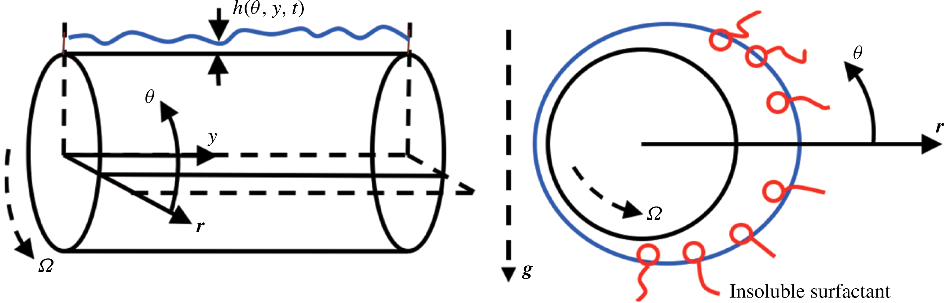
Schematic of problem geometry.

2 Mathematical model
We consider the flow of a thin film of a Newtonian liquid with viscosity
 $\unicode[STIX]{x1D707}$
and density
 $\unicode[STIX]{x1D70C}$
over a cylinder of radius
 $R$
and length
 $L$
(figure 1). The cylinder is assumed to be long enough so that end effects can be neglected. The cylinder rotates counterclockwise around its axis, which is held perpendicular to the gravity vector
 $\boldsymbol{g}$
, at a constant angular speed
 $\unicode[STIX]{x1D6FA}$
. The liquid velocity is expressed as
 $$\begin{eqnarray}\boldsymbol{u}=\unicode[STIX]{x1D714}\boldsymbol{e}_{r}+(r\unicode[STIX]{x1D6FA}+u)\boldsymbol{e}_{\unicode[STIX]{x1D703}}+v\boldsymbol{e}_{y},\end{eqnarray}$$
in cylindrical coordinates (
 $r$
,
 $\unicode[STIX]{x1D703}$
,
 $y$
), where
 $\boldsymbol{e}_{r}$
,
 $\boldsymbol{e}_{\unicode[STIX]{x1D703}}$
and
 $\boldsymbol{e}_{y}$
are the corresponding unit vectors. The liquid is assumed to completely wet the cylinder and is confined to a region
 $R<r\leqslant R+h$
, where the film thickness,
 $h(\unicode[STIX]{x1D703},y,t)$
, is measured from the cylinder surface and is a function of
 $\unicode[STIX]{x1D703}$
,
 $y$
, and time,
 $t$
.
We consider the limiting case where the surfactant is insoluble and its concentration is sufficiently dilute to permit use of a linear equation of state to describe the relationship between surfactant concentration
 $\unicode[STIX]{x1D6E4}(\unicode[STIX]{x1D703},y)$
, and surface tension
 $\unicode[STIX]{x1D70E}(\unicode[STIX]{x1D6E4})$
,
 $$\begin{eqnarray}\unicode[STIX]{x1D70E}=\unicode[STIX]{x1D70E}_{0}+\unicode[STIX]{x1D6E4}\left(\frac{\text{d}\unicode[STIX]{x1D70E}}{\text{d}\unicode[STIX]{x1D6E4}}\right)_{\unicode[STIX]{x1D6E4}=0},\end{eqnarray}$$
where
 $\unicode[STIX]{x1D70E}_{0}$
is the surface tension of a surfactant-free interface.
2.1 Governing equations
The equations of mass and momentum conservation are given by
 $$\begin{eqnarray}\displaystyle & \displaystyle \unicode[STIX]{x1D735}\boldsymbol{\cdot }\boldsymbol{u}=0, & \displaystyle\end{eqnarray}$$
 $$\begin{eqnarray}\displaystyle & \displaystyle \unicode[STIX]{x1D70C}[\boldsymbol{u}_{t}+\boldsymbol{u}\boldsymbol{\cdot }\unicode[STIX]{x1D735}\boldsymbol{u}]=-\unicode[STIX]{x1D735}p+\unicode[STIX]{x1D707}\unicode[STIX]{x1D6FB}^{2}\boldsymbol{u}+\unicode[STIX]{x1D70C}\boldsymbol{g}, & \displaystyle\end{eqnarray}$$
where
 $p$
is pressure and
 $\boldsymbol{g}=-g\sin (\unicode[STIX]{x1D703})\boldsymbol{e}_{r}-g\cos (\unicode[STIX]{x1D703})\boldsymbol{e}_{\unicode[STIX]{x1D703}}$
. For convenience, we define a new radial coordinate
 $z=r-R$
, so all governing equations are solved in the interval
 $0\leqslant z\leqslant h(\unicode[STIX]{x1D703},y,t)$
.
On the cylinder surface,
 $z=0$
, no-slip and no-penetration conditions are applied,
 $$\begin{eqnarray}u=\unicode[STIX]{x1D714}=v=0.\end{eqnarray}$$
At the liquid–air interface,
 $F(\unicode[STIX]{x1D703},y,z,t)=z-h(\unicode[STIX]{x1D703},y,t)=0$
, the liquid needs to satisfy the normal and tangential stress balances and the kinematic condition,
 $$\begin{eqnarray}\displaystyle & \displaystyle -p+2\unicode[STIX]{x1D707}(\boldsymbol{n}\boldsymbol{\cdot }\unicode[STIX]{x1D749}\boldsymbol{\cdot }\boldsymbol{n})=-\unicode[STIX]{x1D70E}\unicode[STIX]{x1D705}, & \displaystyle\end{eqnarray}$$
 $$\begin{eqnarray}\displaystyle & \displaystyle 2\unicode[STIX]{x1D707}(\boldsymbol{n}\boldsymbol{\cdot }\unicode[STIX]{x1D749}\boldsymbol{\cdot }\boldsymbol{t})=\unicode[STIX]{x1D735}_{s}\unicode[STIX]{x1D70E}, & \displaystyle\end{eqnarray}$$
 $$\begin{eqnarray}\displaystyle & \displaystyle \left.\frac{\text{D}F}{\text{D}t}\right|_{z=h(\unicode[STIX]{x1D703},y,t)}=0, & \displaystyle\end{eqnarray}$$
where
 $\boldsymbol{n}$
and
 $\boldsymbol{t}$
are the unit outward normal and tangent vectors,
 $\unicode[STIX]{x1D735}_{s}=(\unicode[STIX]{x1D644}-\boldsymbol{n}\boldsymbol{n})\boldsymbol{\cdot }\unicode[STIX]{x1D735}$
is the surface gradient operator,
 $\unicode[STIX]{x1D644}$
is the identity tensor,
 $\unicode[STIX]{x1D705}=\unicode[STIX]{x1D735}_{s}\boldsymbol{\cdot }\boldsymbol{n}$
is the surface curvature,
 $\unicode[STIX]{x1D749}=[\unicode[STIX]{x1D735}\boldsymbol{u}+(\unicode[STIX]{x1D735}\boldsymbol{u})^{\text{T}}]/2$
is the rate-of-strain tensor and
 $\text{D}/\text{D}t$
is the material derivative.
The surfactant concentration at the liquid–air interface is governed by the following convection–diffusion equation:
 $$\begin{eqnarray}\unicode[STIX]{x1D6E4}_{t}+\unicode[STIX]{x1D735}_{s}\boldsymbol{\cdot }(\boldsymbol{u}_{s}\unicode[STIX]{x1D6E4})+(\unicode[STIX]{x1D735}_{s}\boldsymbol{\cdot }\boldsymbol{n})\unicode[STIX]{x1D6E4}(\boldsymbol{n}\boldsymbol{\cdot }\boldsymbol{u})=D\unicode[STIX]{x1D6FB}_{s}^{2}\unicode[STIX]{x1D6E4},\end{eqnarray}$$
where
 $D$
is the surface diffusivity.
2.2 Scaling
We consider the case where the characteristic film thickness,
 $H$
, is much smaller than the cylinder radius,
 $R$
,
 $\unicode[STIX]{x1D716}\equiv H/R\ll 1$
, so that lubrication theory can be applied. Following Evans et al. (Reference Evans, Schwartz and Roy2004) and Li & Kumar (Reference Li and Kumar2015), we scale velocity with
 $U=\unicode[STIX]{x1D70C}gh^{2}/\unicode[STIX]{x1D707}$
, pressure with
 $P=\unicode[STIX]{x1D707}U/H$
and time with
 $R/U$
, so that
 $$\begin{eqnarray}\left.\begin{array}{@{}c@{}}\displaystyle (z,h)=H(\tilde{z},\tilde{h}),\quad (r,y)=R(\tilde{r},{\tilde{y}})\quad t=T\tilde{t},\\ \displaystyle u=U\tilde{u} ,\quad w=\unicode[STIX]{x1D716}U\tilde{w},\quad v=U\tilde{v},\\ \displaystyle \unicode[STIX]{x1D6E4}=\unicode[STIX]{x1D6E4}_{m}\tilde{\unicode[STIX]{x1D6E4}},\quad \unicode[STIX]{x1D70E}=\unicode[STIX]{x1D70E}_{m}+\tilde{\unicode[STIX]{x1D70E}}\unicode[STIX]{x1D711},\quad p=P\tilde{p}.\end{array}\right\}\end{eqnarray}$$
Here, the dimensionless quantities are denoted with tildes. The terms
 $\unicode[STIX]{x1D6E4}_{m}$
and
 $\unicode[STIX]{x1D70E}_{m}$
are the mean surfactant concentration and the corresponding surface tension, respectively. Since the presence of surfactant lowers the surface tension, the spreading pressure,
 $\unicode[STIX]{x1D711}=\unicode[STIX]{x1D70E}_{0}-\unicode[STIX]{x1D70E}_{m}$
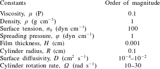
, is a positive constant. Order-of-magnitude of estimates for selected dimensional quantities are listed in table 1. For simplicity, we henceforth drop the tilde notation and all variables are taken to be dimensionless.
Order-of-magnitude estimates of dimensional quantities. The viscosity, density and surface tension are representative of a glycerol–water mixture. The values of surface diffusivities were obtained from the work of Campana & Saita (Reference Campana and Saita2006).

With the above scalings, equations (2.3), (2.4) and (2.9) and the corresponding boundary conditions can be simplified using the lubrication approximation (see appendix A and Evans et al. (Reference Evans, Schwartz and Roy2004), Evans et al. (Reference Evans, Schwartz and Roy2005) and Weidner (Reference Weidner2013) for details), leading to two coupled evolution equations for the film thickness and surfactant concentration. As in the works of Evans et al. (Reference Evans, Schwartz and Roy2004) and Evans et al. (Reference Evans, Schwartz and Roy2005), it is convenient to rescale all lengths with
 $R$
. This yields
 $$\begin{eqnarray}\displaystyle & \displaystyle (1+h)\frac{\unicode[STIX]{x2202}h}{\unicode[STIX]{x2202}t}=-MW\frac{\unicode[STIX]{x2202}}{\unicode[STIX]{x2202}\unicode[STIX]{x1D703}}\left(h+\frac{h^{2}}{2}\right)+\frac{\unicode[STIX]{x2202}}{\unicode[STIX]{x2202}\unicode[STIX]{x1D703}}\left[\left(\frac{h^{3}}{3}+\frac{h^{4}}{2}\right)\cos \unicode[STIX]{x1D703}\right]\hspace{74.00005pt} & \displaystyle \nonumber\\ \displaystyle & \displaystyle \qquad \qquad -\,\overline{\unicode[STIX]{x1D735}}\boldsymbol{\cdot }\left[\frac{h^{3}}{3Bo}\overline{\unicode[STIX]{x1D735}}(h+\overline{\unicode[STIX]{x1D6FB}}^{2}h)+\frac{h^{3}}{3}(W^{2}-\sin \unicode[STIX]{x1D703})\overline{\unicode[STIX]{x1D735}}h-\frac{1}{2}Mah^{2}\overline{\unicode[STIX]{x1D735}}\unicode[STIX]{x1D6E4}\right], & \displaystyle\end{eqnarray}$$
 $$\begin{eqnarray}\displaystyle & \displaystyle r\frac{\unicode[STIX]{x2202}\unicode[STIX]{x1D6E4}}{\unicode[STIX]{x2202}t}+\frac{\unicode[STIX]{x2202}}{\unicode[STIX]{x2202}\unicode[STIX]{x1D703}}(rMW\unicode[STIX]{x1D6E4}+u_{s}\unicode[STIX]{x1D6E4})+\frac{\unicode[STIX]{x2202}}{\unicode[STIX]{x2202}y}[\unicode[STIX]{x1D6E4}v_{s}]+\frac{\unicode[STIX]{x2202}h}{\unicode[STIX]{x2202}t}\unicode[STIX]{x1D6E4}=\frac{1}{Pe}\frac{\unicode[STIX]{x2202}}{\unicode[STIX]{x2202}\unicode[STIX]{x1D703}}\left(\frac{1}{r}\frac{\unicode[STIX]{x2202}\unicode[STIX]{x1D6E4}}{\unicode[STIX]{x2202}\unicode[STIX]{x1D703}}\right)+\frac{1}{Pe}\frac{\unicode[STIX]{x2202}}{\unicode[STIX]{x2202}y}\left(r\frac{\unicode[STIX]{x2202}\unicode[STIX]{x1D6E4}}{\unicode[STIX]{x2202}y}\right), & \displaystyle \nonumber\\ \displaystyle & & \displaystyle\end{eqnarray}$$
where
 $$\begin{eqnarray}\overline{\unicode[STIX]{x1D735}}=\boldsymbol{e}_{\unicode[STIX]{x1D703}}\frac{\unicode[STIX]{x2202}}{\unicode[STIX]{x2202}\unicode[STIX]{x1D703}}+\boldsymbol{e}_{y}\frac{\unicode[STIX]{x2202}}{\unicode[STIX]{x2202}y}\quad \text{and}\quad \overline{\unicode[STIX]{x1D6FB}}^{2}=\frac{\unicode[STIX]{x2202}^{2}}{\unicode[STIX]{x2202}\unicode[STIX]{x1D703}^{2}}+\frac{\unicode[STIX]{x2202}^{2}}{\unicode[STIX]{x2202}y^{2}}.\end{eqnarray}$$
Table 2 gives the definitions, physical meanings and typical values of the dimensionless parameters. Note that operators
 $\overline{\unicode[STIX]{x1D735}}$
and
 $\overline{\unicode[STIX]{x1D6FB}}^{2}$
are not the usual gradient and Laplacian in cylindrical coordinates.
In (2.11) and (2.12), we have neglected terms of
 $O(\unicode[STIX]{x1D716}^{2})$
and higher. The surface velocity,
 $(u_{s},v_{s})=(u,v)|_{z=h}$
, is
 $$\begin{eqnarray}\left.\begin{array}{@{}rcl@{}}\displaystyle u_{s}\ & =\ & \displaystyle -\frac{1}{2}h^{2}\cos \unicode[STIX]{x1D703}-\frac{5}{6}h^{3}\cos \unicode[STIX]{x1D703}-Mah\frac{\unicode[STIX]{x2202}\unicode[STIX]{x1D6E4}}{\unicode[STIX]{x2202}\unicode[STIX]{x1D703}}\\ \ & \ & \displaystyle +\,\frac{1}{2}\left\{\frac{h^{2}}{Bo}\frac{\unicode[STIX]{x2202}}{\unicode[STIX]{x2202}\unicode[STIX]{x1D703}}(h+\overline{\unicode[STIX]{x1D6FB}}^{2}h)+h^{2}(W^{2}-\sin \unicode[STIX]{x1D703})\frac{\unicode[STIX]{x2202}h}{\unicode[STIX]{x2202}\unicode[STIX]{x1D703}}\right\},\\ v_{s}\ & =\ & \displaystyle \frac{1}{2}\left\{\frac{h^{2}}{Bo}\frac{\unicode[STIX]{x2202}}{\unicode[STIX]{x2202}y}(h+\overline{\unicode[STIX]{x1D6FB}}^{2}h)+h^{2}(W^{2}-\sin \unicode[STIX]{x1D703})\frac{\unicode[STIX]{x2202}h}{\unicode[STIX]{x2202}y}\right\}-Mah\frac{\unicode[STIX]{x2202}\unicode[STIX]{x1D6E4}}{\unicode[STIX]{x2202}y}.\end{array}\right\}\end{eqnarray}$$
When Marangoni effects are absent (
 $Ma=0$
), equation (2.11) reduces to that obtained by Evans et al. (Reference Evans, Schwartz and Roy2004). In the limiting case where the cylinder is stationary (
 $W=0$
), equations (2.11) and (2.12) are consistent with the evolution equations obtained by Weidner (Reference Weidner2013).
Dimensionless problem parameters.

For a fixed set of problem parameters (
 $W$
,
 $M$
,
 $Bo$
,
 $Pe$
and
 $Ma$
), an alternating direction implicit (ADI) finite-difference method similar to that used in the works of Witelski & Bowen (Reference Witelski and Bowen2003) and Mata & Bertozzi (Reference Mata and Bertozzi2011) is applied to solve (2.11) and (2.12). Following the work of Li & Kumar (Reference Li and Kumar2015), we neglect the fourth term on the left-hand side of (2.12),
 $(\unicode[STIX]{x2202}h/\unicode[STIX]{x2202}t)\unicode[STIX]{x1D6E4}$
, to simplify our numerical scheme. This term arises due to surface stretching, and our simulations show that it only causes small changes in the resulting concentration profiles for the thin coatings considered here.
Second-order centred differences are used to discretize the spatial derivatives, and an iterative procedure is applied at each time step to improve solution accuracy (Mata & Bertozzi Reference Mata and Bertozzi2011). The
 $(\unicode[STIX]{x1D703},y)$
domain is discretized into a mesh of
 $n_{\unicode[STIX]{x1D703}}\times (n_{y}+1)$
grid points with grid spacing
 $\unicode[STIX]{x1D6E5}_{\unicode[STIX]{x1D703}}=\unicode[STIX]{x1D6E5}_{y}=2\unicode[STIX]{x03C0}/n_{\unicode[STIX]{x1D703}}$
and cylinder length
 $L=n_{y}\unicode[STIX]{x1D6E5}_{y}=2\unicode[STIX]{x03C0}n_{y}/n_{\unicode[STIX]{x1D703}}$
. Following the works of Evans et al. (Reference Evans, Schwartz and Roy2004) and Weidner (Reference Weidner2013), no-flux boundary conditions are imposed at the two ends of the cylinder (
 $y=0$
and
 $y=L$
), and periodicity is imposed in the
 $\unicode[STIX]{x1D703}$
direction (
 $h(\unicode[STIX]{x1D703},y)=h(\unicode[STIX]{x1D703}+2\unicode[STIX]{x03C0},y)$
). In our simulations, we choose
 $n_{\unicode[STIX]{x1D703}}=150$
–
 $200$
and
 $n_{y}=250$
–
 $500$
. For each set of
 $n_{\unicode[STIX]{x1D703}}$
and
 $n_{y}$
used to generate the results shown here, increasing the number of grid points did not change the results within graphical accuracy. Typical computation times for a given run ranged from one day to 1 week on a workstation with a 2.8 GHz Intel Xeon processor. We note that there are interesting questions concerning how surfactants influence the rate of convergence towards steady states and the behaviour of shock-like solutions (Badali et al.
Reference Badali, Chugunova, Pelinovsky and Pollack2011; Burchard, Chugunova & Stephens Reference Burchard, Chugunova and Stephens2012), but a detailed investigation of these issues is beyond the scope of the present work.
3 Zero-gravity case
Although the main focus of this paper is on the case where gravitational effects are significant, it is instructive to first consider the case where the cylinder is spinning so rapidly that gravitational effects are negligible. Since it is no longer appropriate to non-dimensionalize (2.11) and (2.12) using gravity, we rescale them using
 $\unicode[STIX]{x1D70E}/\unicode[STIX]{x1D707}$
and
 $\unicode[STIX]{x1D70E}/R$
as the new characteristic velocity and pressure (stress), respectively (Evans et al.
Reference Evans, Schwartz and Roy2004; Sahu & Kumar Reference Sahu and Kumar2014; Li, Carvalho & Kumar Reference Li, Carvalho and Kumar2017a
). The resulting evolution equations become
 $$\begin{eqnarray}\displaystyle & \displaystyle (1+h)\frac{\unicode[STIX]{x2202}h}{\unicode[STIX]{x2202}t}=-\frac{\unicode[STIX]{x1D6FA}\unicode[STIX]{x1D707}R}{\unicode[STIX]{x1D70E}_{m}}\frac{\unicode[STIX]{x2202}h}{\unicode[STIX]{x2202}\unicode[STIX]{x1D703}}-\frac{1}{3}\overline{\unicode[STIX]{x1D735}}\boldsymbol{\cdot }\{h^{3}\overline{\unicode[STIX]{x1D735}}(h+\overline{\unicode[STIX]{x1D6FB}}^{2}h)+h^{3}S\overline{\unicode[STIX]{x1D6FB}}h\}+\frac{1}{2}Ma\overline{\unicode[STIX]{x1D735}}\boldsymbol{\cdot }(h^{2}\overline{\unicode[STIX]{x1D735}}\unicode[STIX]{x1D6E4}),\qquad & \displaystyle\end{eqnarray}$$
 $$\begin{eqnarray}\displaystyle & \displaystyle r\frac{\unicode[STIX]{x2202}\unicode[STIX]{x1D6E4}}{\unicode[STIX]{x2202}t}+\frac{\unicode[STIX]{x2202}}{\unicode[STIX]{x2202}\unicode[STIX]{x1D703}}\left(r\frac{\unicode[STIX]{x1D6FA}\unicode[STIX]{x1D707}R}{\unicode[STIX]{x1D70E}_{m}}\unicode[STIX]{x1D6E4}+u_{s}\unicode[STIX]{x1D6E4}\right)+\frac{\unicode[STIX]{x2202}}{\unicode[STIX]{x2202}y}\left[\unicode[STIX]{x1D6E4}v_{s}\right]=\frac{1}{Pe}\frac{\unicode[STIX]{x2202}}{\unicode[STIX]{x2202}\unicode[STIX]{x1D703}}\left(\frac{1}{r}\frac{\unicode[STIX]{x2202}\unicode[STIX]{x1D6E4}}{\unicode[STIX]{x2202}\unicode[STIX]{x1D703}}\right)+\frac{1}{Pe}\frac{\unicode[STIX]{x2202}}{\unicode[STIX]{x2202}y}\left(r\frac{\unicode[STIX]{x2202}\unicode[STIX]{x1D6E4}}{\unicode[STIX]{x2202}y}\right),\qquad & \displaystyle\end{eqnarray}$$
where the Marangoni number,
 $Ma$
, the Péclet number,
 $Pe$
, and the dimensionless rotation rate (Weber number),
 $S$
, are defined as
 $$\begin{eqnarray}Ma=\unicode[STIX]{x1D711}/\unicode[STIX]{x1D70E}_{m},\quad Pe=R\unicode[STIX]{x1D70E}_{m}/\unicode[STIX]{x1D707}D,\quad S=\unicode[STIX]{x1D70C}\unicode[STIX]{x1D6FA}^{2}R^{3}/\unicode[STIX]{x1D70E}_{m}.\end{eqnarray}$$
3.1 Linear stability analysis
When gravitational forces are absent, a film of constant thickness with a uniform surfactant concentration is a solution of the governing equations. We examine the fate of small perturbations to this solution via a linear stability analysis (LSA), in which the following normal mode decomposition is used for
 $h$
and
 $\unicode[STIX]{x1D6E4}$
,
 $$\begin{eqnarray}\displaystyle & \displaystyle h(x,y,t)=H_{b}+H_{0}\exp (\text{i}k_{\unicode[STIX]{x1D703}}\unicode[STIX]{x1D703}+\text{i}k_{y}y+st), & \displaystyle\end{eqnarray}$$
 $$\begin{eqnarray}\displaystyle & \displaystyle \unicode[STIX]{x1D6E4}(x,y,t)=\unicode[STIX]{x1D6E4}_{b}+\unicode[STIX]{x1D6E4}_{0}\exp (\text{i}k_{\unicode[STIX]{x1D703}}\unicode[STIX]{x1D703}+\text{i}k_{y}y+st), & \displaystyle\end{eqnarray}$$
where
 $H_{b}$
and
 $\unicode[STIX]{x1D6E4}_{b}$
are the base-state values, and
 $H_{0}$
and
 $\unicode[STIX]{x1D6E4}_{0}$
are the perturbation amplitudes, which are assumed to have real-valued wavenumbers
 $k_{\unicode[STIX]{x1D703}}$
and
 $k_{y}$
and growth rate
 $s$
.
Substitution of (3.5) into the linearized versions of (3.1) and (3.2) leads to an eigenvalue problem of the form
 $$\begin{eqnarray}\boldsymbol{A}\left(\begin{array}{@{}c@{}}H_{0}\\ \unicode[STIX]{x1D6E4}_{0}\end{array}\right)=\left(s+\text{i}k_{\unicode[STIX]{x1D703}}\frac{\unicode[STIX]{x1D6FA}\unicode[STIX]{x1D707}R}{\unicode[STIX]{x1D70E}_{m}}\right)\left(\begin{array}{@{}c@{}}H_{0}\\ \unicode[STIX]{x1D6E4}_{0}\end{array}\right),\end{eqnarray}$$
where
 $$\begin{eqnarray}\boldsymbol{A}=\left(\begin{array}{@{}cc@{}}\displaystyle \frac{H_{b}^{3}}{3r_{b}}k^{2}[(1+S)-k^{2}] & \displaystyle -\frac{1}{2r_{b}}Mak^{2}H_{b}^{2}\\ \displaystyle \frac{1}{2r_{b}}H_{b}^{2}\unicode[STIX]{x1D6E4}_{b}k^{2}[(1+S)-k^{2}] & \displaystyle -\frac{1}{r_{b}}\left(MaH_{b}\unicode[STIX]{x1D6E4}_{b}k^{2}+\frac{1}{Pe_{s}}\frac{1}{r_{b}}k_{\unicode[STIX]{x1D703}}^{2}+\frac{1}{Pe_{s}}r_{b}k_{y}^{2}\right)\end{array}\right).\end{eqnarray}$$
Here,
 $k=(k_{\unicode[STIX]{x1D703}}^{2}+k_{y}^{2})^{1/2}$
and
 $r_{b}=1+H_{b}$
. The two values of the growth rate can be determined analytically, but we do not show the expressions for brevity. It turns out that both values of
 $s$
are purely real, but only one of them is positive over a range of wavenumbers and it is this value which is discussed below.
It is useful to first consider separately the cases of purely angular and purely axial perturbations when Marangoni stresses are absent (
 $Ma=0$
). Purely angular perturbations (
 $k_{y}=0$
) were considered by Evans et al. (Reference Evans, Schwartz and Roy2004), and the corresponding growth rate is
 $$\begin{eqnarray}s_{\unicode[STIX]{x1D703}}={\textstyle \frac{1}{3}}H_{b}^{3}((1+S)k_{\unicode[STIX]{x1D703}}^{2}-k_{\unicode[STIX]{x1D703}}^{4}).\end{eqnarray}$$
Angular perturbations with
 $k_{\unicode[STIX]{x1D703}}<k_{\unicode[STIX]{x1D703}}^{cutoff}$
have positive growth rates and grow in amplitude due to centrifugal forces, while those with
 $k_{\unicode[STIX]{x1D703}}>k_{\unicode[STIX]{x1D703}}^{cutoff}$
have negative growth rates and decay due to surface tension. The cutoff wavenumber,
 $k_{\unicode[STIX]{x1D703}}^{cutoff}$
, and the most dangerous wavenumber,
 $k_{\unicode[STIX]{x1D703}}^{max}$
, are
 $$\begin{eqnarray}\displaystyle & \displaystyle k_{\unicode[STIX]{x1D703}}^{cutoff}=[\sqrt{1+S}], & \displaystyle\end{eqnarray}$$
 $$\begin{eqnarray}\displaystyle & \displaystyle k_{\unicode[STIX]{x1D703}}^{max}=[\sqrt{(1+S)/2}], & \displaystyle\end{eqnarray}$$
where
 $[x]$
is the greatest integer less than or equal to
 $x$
. (Due to periodicity,
 $k_{\unicode[STIX]{x1D703}}$
is restricted to integer values.) Note that when
 $S=0$
(stationary cylinder), purely angular perturbations do not grow.
For purely axial perturbations (
 $k_{\unicode[STIX]{x1D703}}=0$
), it turns out that the growth rate has the same expression with
 $k_{y}$
in place of
 $k_{\unicode[STIX]{x1D703}}$
, i.e.
 $s_{y}=(1/3)H_{b}^{3}((1+S)k_{y}^{2}-k_{y}^{4})$
. The cutoff wavenumber is
 $k_{y}^{cutoff}=\sqrt{1+S}$
and the most dangerous wavenumber is
 $k_{y}^{max}=\sqrt{(1+S)/2}$
. In contrast to purely angular perturbations, purely axial perturbations can grow when
 $S=0$
, which corresponds to the Rayleigh–Plateau instability. When
 $S=0$
, perturbations having a wavelength longer than the cylinder circumference will tend to grow. When
 $S\neq 0$
, centrifugal forces further destabilize perturbations, causing the growth rates to increase and the band of unstable wavenumbers to widen.
When Marangoni stresses are present, we can no longer obtain analytical expressions for the cutoff and most dangerous wavenumbers. The case of purely angular perturbations (
 $k_{y}=0$
) was considered by Li & Kumar (Reference Li and Kumar2015), and it was found that surfactant-induced Marangoni stresses reduce the growth rates but do not significantly change the cutoff and most dangerous wavenumbers. This occurs because the surfactant concentration perturbations are in phase with the interface perturbations, lowering the surface tension at the interface crests relative to the troughs. The resulting Marangoni stresses then drive a flow back to the troughs, thereby reducing the instability growth rates. We have conducted a similar analysis for purely axial perturbations (
 $k_{\unicode[STIX]{x1D703}}=0$
) and observe the same behaviour. Rather than showing detailed results here, we refer the reader to the supplementary material available at https://doi.org/10.1017/jfm.2018.153.
3.2 Nonlinear evolution
We now turn to the nonlinear evolution of the instabilities discussed in § 3.1. The finite-difference scheme described in § 2 was validated by comparison with the LSA results of § 3.1. Excellent agreement was observed for both purely angular and purely axial perturbations for both
 $Ma=0$
and
 $Ma\neq 0$
(results not shown). Here, we examine what happens when perturbations in both directions grow simultaneously using a representative set of problem parameters. The following initial condition is used:
 $$\begin{eqnarray}h(\unicode[STIX]{x1D703},y,t=0)=h_{0}(1+\unicode[STIX]{x1D6FC}\cos (k_{\unicode[STIX]{x1D703}}\unicode[STIX]{x1D703})+\unicode[STIX]{x1D6FC}\cos (k_{y}y)),\end{eqnarray}$$
where
 $\unicode[STIX]{x1D6FC}$
denotes the perturbation amplitude and
 $h_{0}$
denotes the mean film thickness.
We first set
 $Ma=0$
and consider an initial perturbation with
 $k_{\unicode[STIX]{x1D703}}=2<k_{\unicode[STIX]{x1D703}}^{max}=3$
and
 $k_{y}=k_{y}^{max}=3$
. To gain insight into how the flow transports surfactant, we also calculate the concentration field
 $\unicode[STIX]{x1D6E4}$
even though it does not influence the film shape when
 $Ma=0$
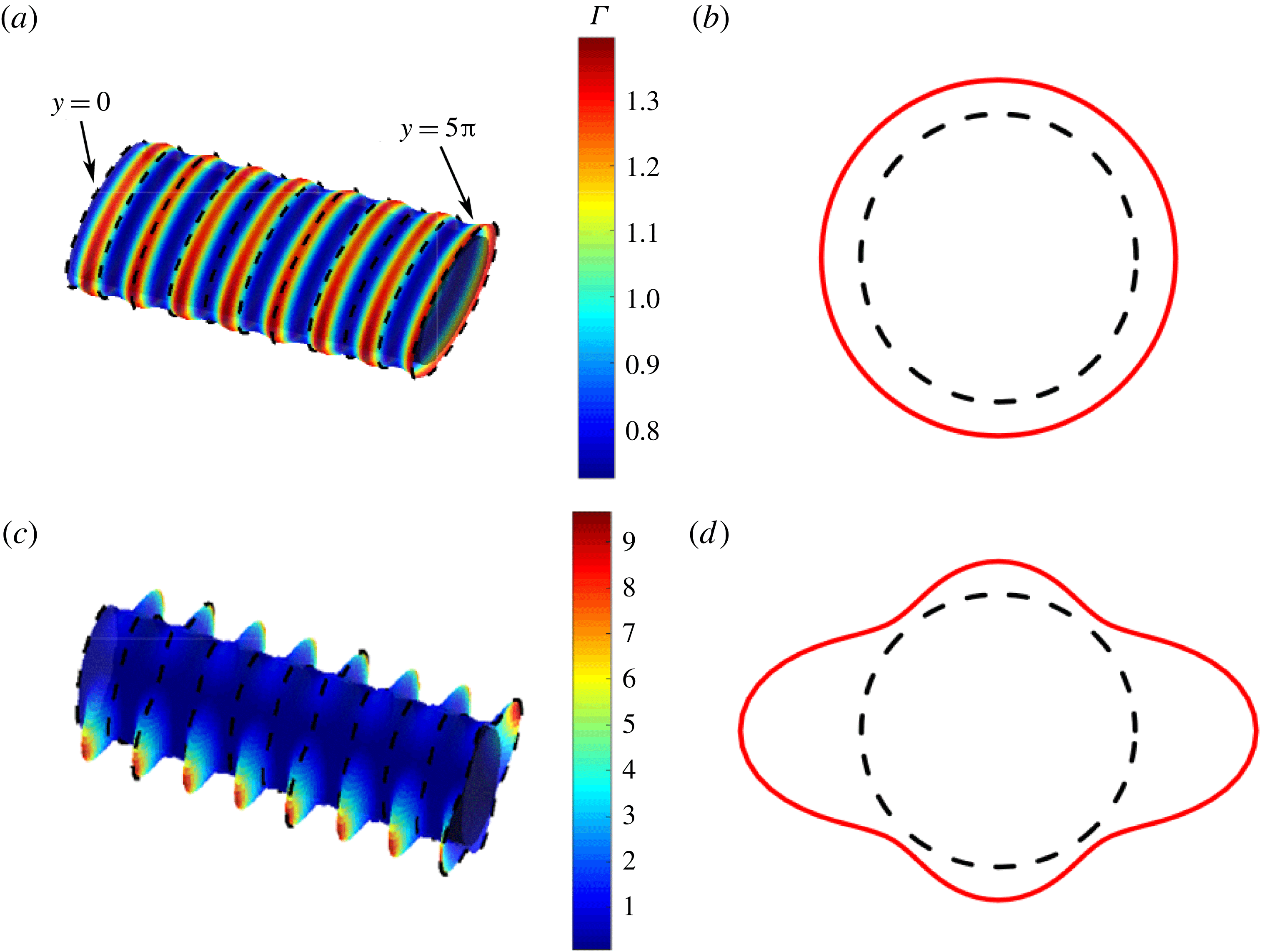
. The evolution of the film follows two distinct stages, and we show in figure 2(a,c) the free-surface profiles and surfactant distributions in these two stages. For ease of visualization, the corresponding free-surface profiles around the cylinder circumference at
 $y=0$
(marked in figure 2
a) are shown in figure 2(b,d) with red solid lines.
(a,c) Free-surface profiles and surfactant distributions in the zero-gravity case with
 $h_{0}=0.03162$
,
 $\unicode[STIX]{x1D6FC}=10^{-5}$
,
 $k_{y}=3$
,
 $k_{\unicode[STIX]{x1D703}}=2$
,
 $S=20$
,
 $Ma=0$
and
 $Pe=10^{5}$
at (a)
 $t=7\times 10^{3}$
and (c)
 $t=10^{4}$
. The corresponding free-surface profiles around the cylinder circumference at
 $y=0$
are plotted in (b,d) with red solid lines. The black dashed lines indicate the cylinder surface. For ease of visualization, the thickness plotted in (a–d) is five times larger than the actual value. The spacing between the dashed lines in (a,c) is
 $0.5\unicode[STIX]{x03C0}$
.

During the early stage (figure 2
a), 7.5 rings develop along the axis (
 $k_{y}\times L/2\unicode[STIX]{x03C0}=7.5$
), while the coating stays almost axisymmetric (figure 2
b). This is simply because the initial perturbation has a higher growth rate in the axial direction. As these rings grow in size, they become unstable to angular perturbations in the later stage and each of them breaks into two liquid droplets (
 $k_{\unicode[STIX]{x1D703}}=2$
) connected by relatively thin films as shown in figure 2(c,d). The growth of these droplets leads to a highly distorted free-surface shape, which significantly increases computational costs, and for this reason, we are unable to find a steady state with our lubrication model.
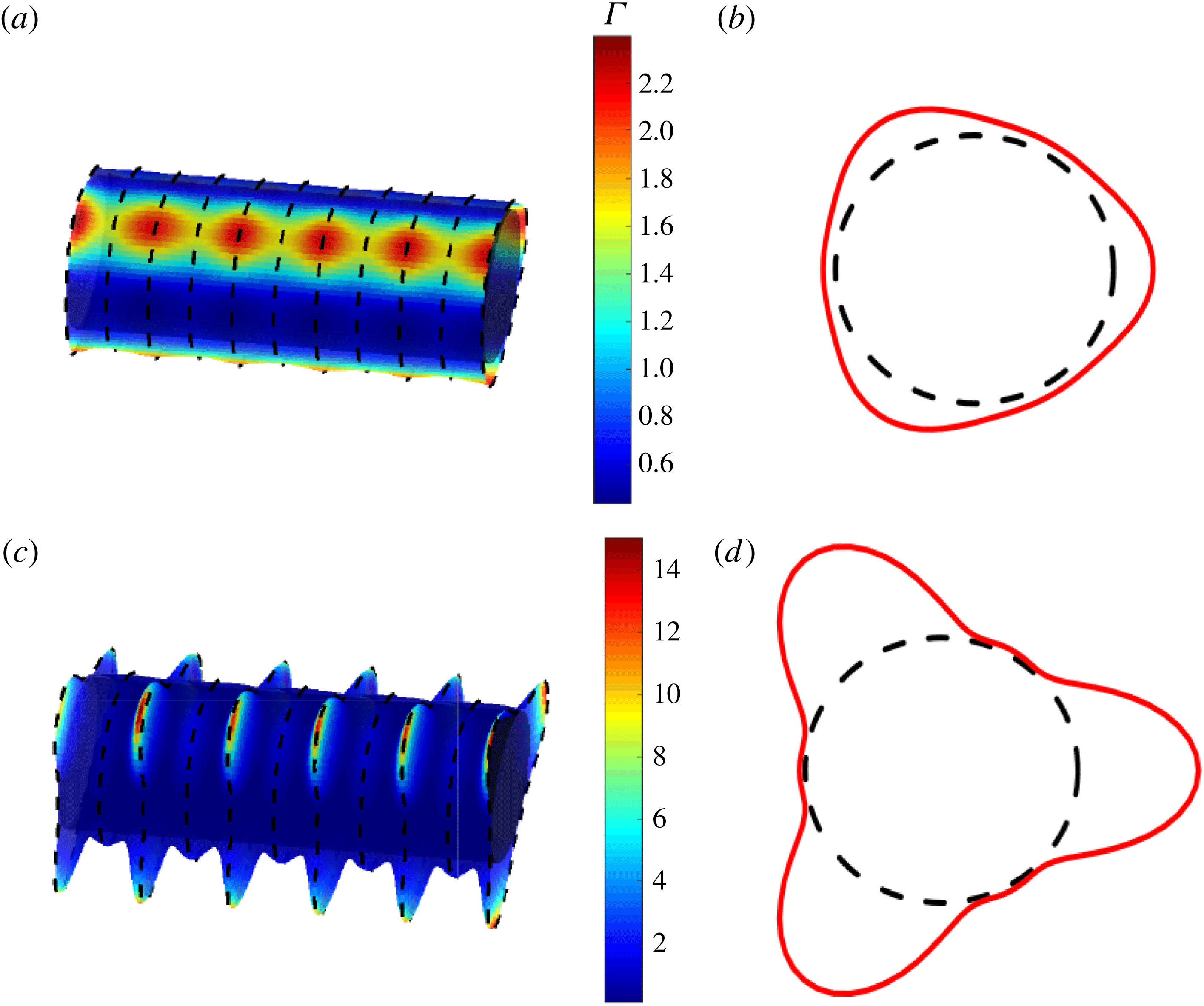
(a,c) Free-surface profiles and surfactant distributions in the zero-gravity case with
 $h_{0}=0.03162$
,
 $\unicode[STIX]{x1D6FC}=10^{-5}$
,
 $k_{y}=2$
,
 $k_{\unicode[STIX]{x1D703}}=3$
,
 $S=20$
,
 $Ma=0$
and
 $Pe=10^{5}$
at (a)
 $t=7\times 10^{3}$
and (c)
 $t=10^{4}$
. The corresponding free-surface profiles around the cylinder circumference at
 $y=0$
are plotted in (b,d) with red dashed lines. The black dashed lines indicate the cylinder surface. For ease of visualization, the thickness plotted in (a–d) is five times larger than the actual value. The spacing between the dashed lines in (a,c) is
 $0.5\unicode[STIX]{x03C0}$
.

For an initial perturbation with
 $k_{\unicode[STIX]{x1D703}}=3$
and
 $k_{y}=2$
, the evolution of the coating also follows two distinct stages. The corresponding free-surface profiles and surfactant distributions at
 $t=7\times 10^{3}$
and
 $t=10^{4}$
are shown in figure 3, along with the free-surface profiles around the cylinder circumference at
 $y=0$
. In this case, three ridges (
 $k_{\unicode[STIX]{x1D703}}=3$
) aligned with the cylinder axis develop at the early stage (figure 3
b) with relatively small axial variations in film thickness (figure 3
a). As more liquid is driven into the ridges by centrifugal forces, the growth of axial perturbations is promoted and each ridge breaks into five droplets (
 $k_{y}\times L/2\unicode[STIX]{x03C0}=5$
) in the later stage, as shown in figure 3(c,d).
Figures 2(a,c) and 3(a,c) clearly show that the regions where the film is thicker also appear to be the high-concentration (red) regions. Thus, the convective flows triggered by centrifugal forces tend to drive surfactant to the thick-film regions, giving rise to concentration gradients at the free surface. This suggests that when
 $Ma\neq 0$
, the resulting Marangoni stresses will drive liquid away from the thick-film (lower-surface-tension) regions to the thin-film (higher-surface-tension) regions and thus suppress the growth rates of both the angular and axial perturbations. Results from our nonlinear simulations confirm this but are not shown here for brevity. We note that for
 $Ma=0$
, the surfactant concentration should eventually become uniform if the coating reaches a steady state in which all flows vanish. However, as mentioned earlier, we are unable to reach steady states in these simulations.
4 Stable speed window (
 $Ma=0$
) and its disappearance (
$Ma\neq 0$
)


We now incorporate the effects of gravity to show the presence of a stable speed window when
 $Ma=0$
, first reported by Evans et al. (Reference Evans, Schwartz and Roy2005) (§ 1). Within this window, which occurs at moderate rotation rates, the film stays axially uniform (Evans et al.
Reference Evans, Schwartz and Roy2005). At low rotation rates, the film is susceptible to the Rayleigh–Taylor (RT) instability and droplets form near the bottom of the cylinder. At high rotation rates, the film is susceptible to the Rayleigh–Plateau (RP) instability and rings form around the cylinder. We also demonstrate here that the presence of Marangoni stresses can cause the stable speed window to disappear.
Following the work of Evans et al. (Reference Evans, Schwartz and Roy2005), we consider a rotating cylinder with dimensional radius
 $R=l_{c}$
 $(Bo=1)$
, where
 $l_{c}=\sqrt{\unicode[STIX]{x1D70E}_{m}/\unicode[STIX]{x1D70C}g}$
is the capillary length. For a glycerol–water mixture (table 1), the corresponding values are
 $l_{c}=R=0.2~\text{cm}$
. As in the work of Evans et al. (Reference Evans, Schwartz and Roy2005), we perform simulations for a film with mean thickness
 $h_{0}=0.03162$
and dimensionless viscosity
 $M=0.007$
(table 2). The corresponding dimensionless critical rotation rate (1.1) is
 $W_{c}=2.01h_{0}^{2}/M=0.29$
(
 $\unicode[STIX]{x1D6FA}_{c}=20~\text{s}^{-1}$
in dimensional form). Above this rotation rate, a smooth coating can be formed (§ 1). Equations (2.11) and (2.12) are solved with initial condition
 $$\begin{eqnarray}h(\unicode[STIX]{x1D703},y,0)=h_{0}\left[1+\unicode[STIX]{x1D6FC}_{y}\cos \left(\frac{2\unicode[STIX]{x03C0}y}{\unicode[STIX]{x1D706}}\right)\right],\end{eqnarray}$$
which corresponds to an axisymmetric coating with a half-cosine variation in the axial direction. Here,
 $\unicode[STIX]{x1D6FC}_{y}=0.001$
is the perturbation amplitude and
 $\unicode[STIX]{x1D706}$
is the wavelength of the perturbation.
Similar to the zero-gravity case, perturbations with wavelength longer than a cutoff value,
 $\unicode[STIX]{x1D706}_{cutoff}$
, grow in amplitude at a given rotation rate, while those with
 $\unicode[STIX]{x1D706}<\unicode[STIX]{x1D706}_{cutoff}$
decay. Thus, for a given value of
 $W$
, varying
 $\unicode[STIX]{x1D706}$
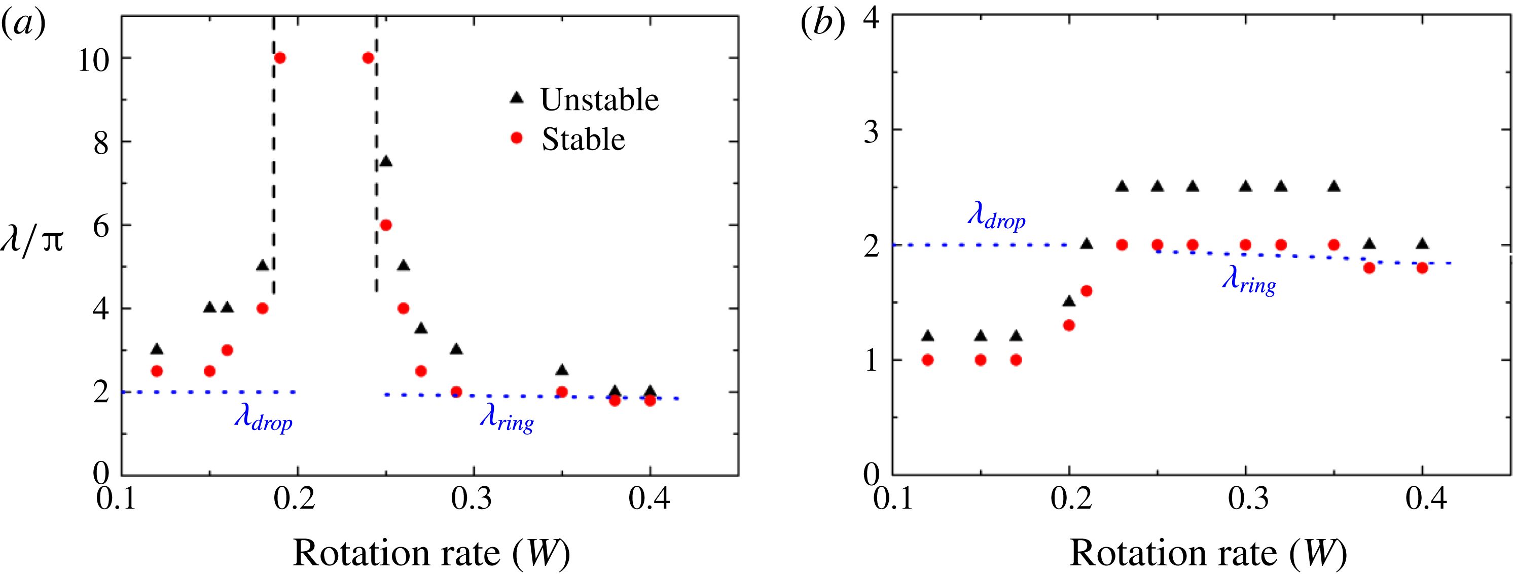
in the initial condition allows us to approximately locate the cutoff wavelength. Results of our numerical simulations are shown in figure 4(a), where the red dots denote the largest stable wavelength, and the black triangles denote the smallest unstable wavelength. This stability diagram is in good agreement with that obtained by Evans et al. (Reference Evans, Schwartz and Roy2005). We note that between the largest stable wavelength and the smallest unstable wavelength, we are unable to confidently determine whether perturbations grow or decay.
Stability diagram for a coating on a rotating cylinder with
 $Bo=1$
,
 $h_{0}=0.03162$
,
 $M=0.007$
and (a)
 $Ma=0$
and (b)
 $Ma=0.001$
and
 $Pe=10^{5}$
. Blue dashed lines denote the cutoff wavelength obtained from a linear stability analysis (for
 $Ma=0$
). The black dotted vertical lines in (a) correspond to
 $W=0.186$
and
 $W=0.242$
.

It is instructive to compare the cutoff wavelengths in figure 4(a) with known results for the RT and RP instabilities, as done by Evans et al. (Reference Evans, Schwartz and Roy2005). For an axisymmetric coating on a cylinder, the cutoff wavelength for the RP (ring-type) instability is
 $\unicode[STIX]{x1D706}_{ring}=2\unicode[STIX]{x03C0}/k^{cutoff}=2\unicode[STIX]{x03C0}/\sqrt{1+S}$
(§ 3.1). For a thin layer of liquid underneath a planar substrate (see supplementary material), the cutoff wavelength for the RT (droplet-type) instability is
 $\unicode[STIX]{x1D706}_{drop}=2\unicode[STIX]{x03C0}/\sqrt{Bo}$
. We plot in figure 4(a)
 $\unicode[STIX]{x1D706}_{ring}$
and
 $\unicode[STIX]{x1D706}_{drop}$
as functions of
 $W$
with blue dashed lines.
Figure 4(a) shows that the cutoff wavelength from the simulations is in good agreement with
 $\unicode[STIX]{x1D706}_{ring}$
in the RP regime (high rotation rates), but is always slightly larger than
 $\unicode[STIX]{x1D706}_{drop}$
in the RT regime (low rotation rates), possibly due to the planar geometry on which
 $\unicode[STIX]{x1D706}_{drop}$
is based. At moderate rotation rates, the cutoff wavelength increases dramatically, and even perturbations with wavelength
 $\unicode[STIX]{x1D706}=10\unicode[STIX]{x03C0}$
(the longest wavelength tested in our simulations) are found to be stable for
 $0.186<W<0.242$
, suggesting that axial perturbations are unlikely to grow. The physical mechanisms responsible for this window are discussed in § 5.
While computational limitations have prevented us from performing a comprehensive parametric study, we speculate that the stable speed window may not exist if gravitational forces become sufficiently strong relative to surface-tension forces, which could happen if
 $Bo$
or the initial film thickness is too large. Limited simulations performed by Evans et al. indicate that an increase in
 $M$
shifts the stable speed window to lower rotation rates, presumably since a lower rotation rate is required in a more viscous liquid to obtain a film of comparable thickness (Evans et al.
Reference Evans, Schwartz and Roy2005). This suggests that if
 $M$
is large enough, the stable speed window may not be present in the range of rotation rates considered. Indeed, the results of some limited simulations we have performed appear consistent with this conjecture.
We now examine the influence of Marangoni stresses and consider a representative case where
 $Ma=0.001$
and
 $Pe=10^{5}$
. All simulations are started with uniform surface concentration
 $\unicode[STIX]{x1D6E4}=1$
, and the stability diagram is shown in figure 4(b). Also shown with blue dashed lines are predictions of
 $\unicode[STIX]{x1D706}_{ring}$
and
 $\unicode[STIX]{x1D706}_{drop}$
when
 $Ma=0$
, since LSA reveals that Marangoni stresses have very little influence on these values (see the supplementary material).
In the regime where the RP instability dominates (
 $W>0.3$
), the corresponding cutoff wavelength is in good agreement with
 $\unicode[STIX]{x1D706}_{ring}$
, similar to the
 $Ma=0$
case. In the regime where the RT instability dominates (
 $W<0.2$
), Marangoni stresses lower the cutoff value to approximately
 $\unicode[STIX]{x1D706}_{ring}/2$
. For all the rotation rates considered in our simulations (
 $0.1<W<0.5$
), a minimum unstable wavelength above which the initial perturbations grow in amplitude can always be found. Marangoni stresses can thus cause the stable speed window to vanish. The mechanisms underlying this are discussed in § 6.
5 Surfactant-free case (
$Ma=0$
)

As noted in § 1, although the stable speed window for
 $Ma=0$
(§ 4) has been observed, the mechanisms underlying it are still unknown, and one purpose of the present paper is to understand these mechanisms. In doing so, it is useful to integrate (A 24) from
 $z=0$
to
 $z=h$
to study the axial flux,
 $Q_{y}$
(which depends on
 $y$
,
 $\unicode[STIX]{x1D703}$
and
 $t$
), given by
 $$\begin{eqnarray}\displaystyle & \displaystyle Q_{y}^{G/\unicode[STIX]{x1D6FA}}=\frac{1}{3}h^{3}\left((W^{2}-\sin \unicode[STIX]{x1D703})\frac{\unicode[STIX]{x2202}h}{\unicode[STIX]{x2202}y}\right), & \displaystyle\end{eqnarray}$$
 $$\begin{eqnarray}\displaystyle & \displaystyle Q_{y}^{\unicode[STIX]{x1D70E}}=\frac{1}{3Bo}h^{3}\left(\left(\frac{\unicode[STIX]{x2202}h}{\unicode[STIX]{x2202}y}+\frac{\unicode[STIX]{x2202}^{3}h}{\unicode[STIX]{x2202}y^{3}}\right)+\frac{\unicode[STIX]{x2202}}{\unicode[STIX]{x2202}y}\left(\frac{\unicode[STIX]{x2202}^{2}h}{\unicode[STIX]{x2202}\unicode[STIX]{x1D703}^{2}}\right)\right), & \displaystyle\end{eqnarray}$$
 $$\begin{eqnarray}\displaystyle & \displaystyle Q_{y}=Q_{y}^{G/\unicode[STIX]{x1D6FA}}+Q_{y}^{\unicode[STIX]{x1D70E}}, & \displaystyle\end{eqnarray}$$
where
 $Q_{y}^{G/\unicode[STIX]{x1D6FA}}$
denotes the contribution from centrifugal forces (term with
 $W^{2}$
) and gravitational forces (term with
 $\sin \unicode[STIX]{x1D703}$
), and
 $Q_{y}^{\unicode[STIX]{x1D70E}}$
denotes the contribution from surface-tension forces. Positive values of
 $Q_{y}$
correspond to an axial flux in the positive
 $y$
-direction (figure 1
a). We investigate the axial flux in both the low-
 $W$
region (where the RT instability dominates) and the high-
 $W$
region (where the RP instability dominates).
(a) Film thickness and (c,e,g) axial flux along the cylinder circumference at
 $y=\unicode[STIX]{x03C0}$
and
 $t=4\times 10^{6}$
with
 $L=5\unicode[STIX]{x03C0}$
,
 $Bo=1$
,
 $h_{0}=0.03162$
,
 $M=0.007$
,
 $Ma=0$
and
 $W=0.1$
. The corresponding free-surface profiles are shown in (b), (d), (f) and (g), where the thickness plotted is five times larger than the actual value for ease of visualization. Red arrows indicate the direction and strength of the axial flux at
 $y=\unicode[STIX]{x03C0}$
.

5.1 Rayleigh–Taylor instability
In the regime where the RT instability dominates (left side of the stable speed window in figure 4
a), the film sags due to gravity-driven drainage and forms a ridge of liquid aligned with the cylinder axis (Evans et al.
Reference Evans, Schwartz and Roy2005). This ridge is unstable and tends to break up into droplets underneath the cylinder. These droplets grow in size until the coating reaches a steady state. We pick a representative rotation rate
 $W=0.1$
(in the RT-instability region in figure 4
a), and perform simulations with a layer of nearly uniform thickness with random noise added,
 $$\begin{eqnarray}h(\unicode[STIX]{x1D703},y,t=0)=h_{0}(1+0.01[R_{\unicode[STIX]{x1D703},y}-{\textstyle \frac{1}{2}}]),\end{eqnarray}$$
where
 $R_{\unicode[STIX]{x1D703},y}$
is a randomly chose value between
 $0$
and
 $1$
for each value of
 $\unicode[STIX]{x1D703}$
and
 $y$
.
The steady film-thickness profile at
 $t=4\times 10^{6}$
and the corresponding axial flux and its contributions are plotted in figure 5(a,c,e,g), respectively, as functions of angular position at
 $y=\unicode[STIX]{x03C0}$
. Figure 5(b) shows the full free-surface profile observed from the cylinder front. Figure 5(d,f,h) shows the same free-surface profile but only at the lower half of the cylinder, where large variations in free-surface curvature occur.
As shown in figure 5(b), two distinct half-droplets of almost the same size develop near the bottom at the two ends of the cylinder. The corresponding film thickness around the circumference of the cylinder at
 $y=\unicode[STIX]{x03C0}$
is shown in figure 5(a). The thickness profile on the downward-moving side of the droplet (
 $\unicode[STIX]{x03C0}<\unicode[STIX]{x1D703}<1.5\unicode[STIX]{x03C0}$
) is steeper than that on the upward-moving side of the droplet (
 $1.5\unicode[STIX]{x03C0}<\unicode[STIX]{x1D703}<2\unicode[STIX]{x03C0}$
) due to the effects of cylinder rotation, and the thickness reaches its maximum (denoted with a dashed line) slightly above the bottom of the cylinder (
 $\unicode[STIX]{x1D703}=1.5\unicode[STIX]{x03C0}$
).
For
 $W=0.1$
, the centrifugal term in (5.1) is negligible relative to the gravitational term, and the flux arising due to gravity (
 $Q_{y}^{G/\unicode[STIX]{x1D6FA}}$
shown in figure 5
c,d) is negative around cylinder circumference, indicating that gravitational forces tend to drive liquid to the thick-film regions (i.e. droplets). The strongest flux occurs at the point of maximum film thickness, which also corresponds to the point where gravitational forces acting on the liquid are the strongest.
The flux arising due to surface-tension forces (
 $Q_{y}^{\unicode[STIX]{x1D70E}}$
shown in figure 5
e,f) is positive on the downward-moving side of the droplet, but changes sign in a small region on the upward-moving side. This suggests that surface tension acts mainly as a stabilizing force, driving liquid to the thin-film region (i.e. middle of the cylinder). The strongest flux occurs on the downward-moving side of the droplet, slightly ahead of the point of maximum film thickness.
The resulting total flux (
 $Q_{y}=Q_{y}^{G/\unicode[STIX]{x1D6FA}}+Q_{y}^{\unicode[STIX]{x1D70E}}$
shown in figure 5
g,h) changes sign at the point of maximum film thickness, and is positive on the upward-moving side of the droplet and negative on the downward-moving side. This implies that gravitational forces dominate on the upward-moving side, while surface-tension forces dominate on the downward-moving side. The competition between them determines whether the initial axial perturbation will grow or decay. The areas of regions
 $I$
and
 $II$
marked in figure 5(e),
 $A_{I}$
, and
 $A_{II}$
, measure how much flux crosses over the
 $y=\unicode[STIX]{x03C0}$
plane on the upward-moving side and on the downward-moving side, respectively. For
 $W=0.1$
, our numerical results (not shown here for brevity) reveal that
 $A_{II}$
is always greater than
 $A_{I}$
during the early transient stage, so droplets tend to grow in size under the action of gravity until the coating reaches a steady state (figure 5
b) where
 $A_{I}=A_{II}$
.
An increase in the value of
 $W$
causes a decrease in the size of the ridge (Evans et al.
Reference Evans, Schwartz and Roy2004; Li & Kumar Reference Li and Kumar2015), which corresponds to a smaller amount of liquid inside the ridge and therefore weaker destabilizing gravitational forces acting on the ridge. In this case, the flux arising due to gravity-driven drainage is not strong enough to compensate the liquid loss in the droplet caused by surface-tension-induced flow. This explains why the coating becomes more stable (larger cutoff wavelength) to axial perturbations with an increase in the rotation rate (near
 $W=0.186$
in figure 4
a) in the region where the RT instability dominates.
Further calculations reveal that
 $(h_{\unicode[STIX]{x1D703}\unicode[STIX]{x1D703}})_{y}$
is the dominant term in (5.2); this term arises from both angular and axial variations in the angular curvature. To understand why the effects of surface tension are especially strong on the downward-moving side of the droplet (figure 5
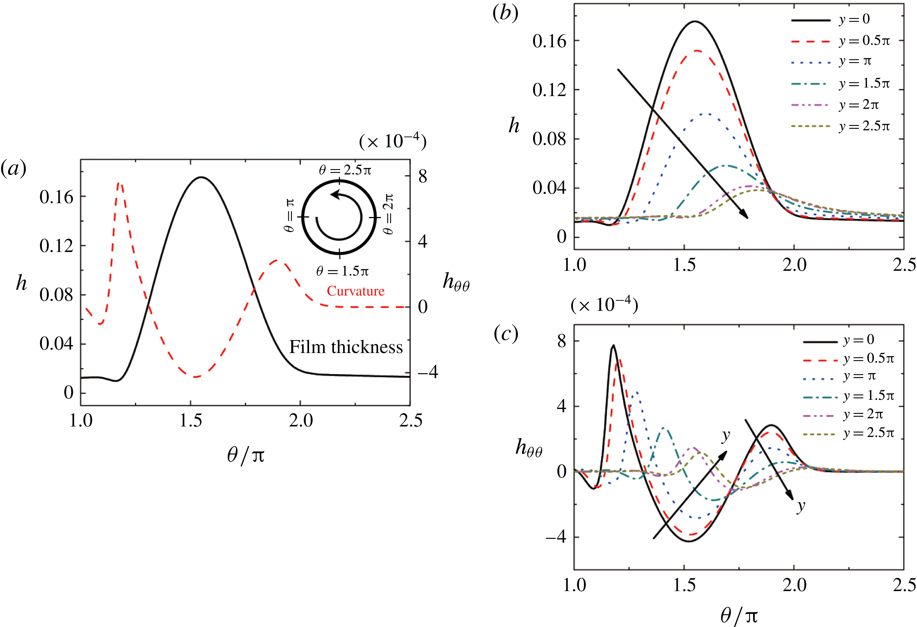
e,f), we plot in figure 6(
 $h$
) and
 $h_{\unicode[STIX]{x1D703}\unicode[STIX]{x1D703}}$
for
 $\unicode[STIX]{x03C0}<\unicode[STIX]{x1D703}<2.5\unicode[STIX]{x03C0}$
(marked in figure 6
a) at different positions along the cylinder axis for the simulation shown in figure 5. We choose the region
 $\unicode[STIX]{x03C0}<\unicode[STIX]{x1D703}<2.5\unicode[STIX]{x03C0}$
because large variations in
 $h$
and
 $h_{\unicode[STIX]{x1D703}\unicode[STIX]{x1D703}}$
occur in this region.
Film thickness (
 $h$
) and its second derivative in the angular direction (
 $h_{\unicode[STIX]{x1D703}\unicode[STIX]{x1D703}}$
) at (a)
 $y=0$
and (b,c) at other values of
 $y$
with
 $Bo=1$
,
 $h_{0}=0.03162$
,
 $M=0.007$
,
 $L=5\unicode[STIX]{x03C0}$
,
 $Ma=0$
and
 $W=0.1$
at
 $t=4\times 10^{6}$
.

For
 $y=0$
,
 $h_{\unicode[STIX]{x1D703}\unicode[STIX]{x1D703}}$
(red dashed line in figure 6
a) is almost zero near the cylinder top (
 $2\unicode[STIX]{x03C0}<\unicode[STIX]{x1D703}<2.5\unicode[STIX]{x03C0}$
) where the film is very thin due to gravity-driven drainage. In the thick-film region (
 $1.25\unicode[STIX]{x03C0}<\unicode[STIX]{x1D703}<2\unicode[STIX]{x03C0}$
),
 $h_{\unicode[STIX]{x1D703}\unicode[STIX]{x1D703}}$
decreases on the downward-moving side of the droplet (
 $1.25\unicode[STIX]{x03C0}<\unicode[STIX]{x1D703}<1.5\unicode[STIX]{x03C0}$
), increases on the upward-moving side (
 $1.5\unicode[STIX]{x03C0}<\unicode[STIX]{x1D703}<2\unicode[STIX]{x03C0}$
), and reaches both its maximum and minimum on the downward-moving side.
Figure 6(b) shows that the maximum film thickness around cylinder circumference at a given value of
 $y$
decreases with an increase in
 $y$
(closer to the middle of the cylinder), since gravitational forces draw liquid to both ends of the cylinder (
 $y=0$
). The increase in
 $y$
also causes the point of maximum thickness to rise higher (larger
 $\unicode[STIX]{x1D703}$
). This phenomenon can be explained by noticing that the point of maximum thickness is determined by the interplay between viscous drag and gravity. A smaller maximum thickness corresponds to weaker gravitational forces there, and as a result, viscous-drag forces push the point of maximum thickness upward, closer to the cylinder symmetry plane (
 $\unicode[STIX]{x1D703}=0$
).
Since the minimum value of
 $h_{\unicode[STIX]{x1D703}\unicode[STIX]{x1D703}}$
occurs near the point of maximum thickness (figure 6
a), the location of this minimum also rises higher with an increase in
 $y$
(figure 6
c). As a result, the value of
 $h_{\unicode[STIX]{x1D703}\unicode[STIX]{x1D703}}$
increases with an increase in
 $y$
(yielding a positive value of
 $(h_{\unicode[STIX]{x1D703}\unicode[STIX]{x1D703}})_{y}$
) on the downward-moving side of the droplet (
 $1.25\unicode[STIX]{x03C0}<\unicode[STIX]{x1D703}<1.75\unicode[STIX]{x03C0}$
), while it decreases (yielding a negative value of
 $(h_{\unicode[STIX]{x1D703}\unicode[STIX]{x1D703}})_{y}$
) in a small region on the upward-moving side (
 $1.75\unicode[STIX]{x03C0}<\unicode[STIX]{x1D703}<2\unicode[STIX]{x03C0}$
). The variation in
 $h_{\unicode[STIX]{x1D703}\unicode[STIX]{x1D703}}$
is more significant on the downward-moving side than elsewhere, and this gives rise to a strong flux there in the positive
 $y$
-direction (figure 5
e). This flux stabilizes the coating by driving liquid back to the middle of the cylinder.
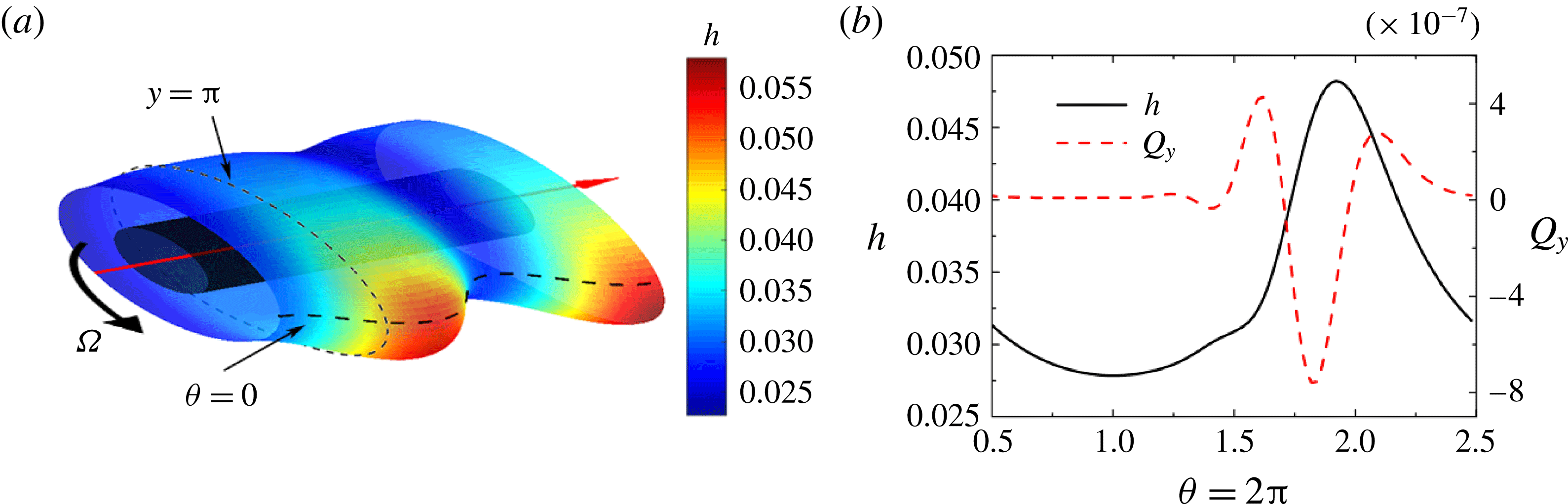
(a) Free-surface profile at
 $t=4\times 10^{6}$
with
 $L=5\unicode[STIX]{x03C0}$
,
 $Bo=1$
,
 $h_{0}=0.03162$
,
 $M=0.007$
,
 $Ma=0$
and
 $W=0.3$
. (b) Film thickness and total axial flux (
 $Q_{y}$
) at
 $y=\unicode[STIX]{x03C0}$
(marked in a). For ease of visualization, the thickness plotted in (a) is 50 times larger than the actual value.

5.2 Rayleigh–Plateau instability
We now turn to the regime where the RP instability dominates (right side of the stable speed window in figure 4
a). In this regime, a Moffatt-type smooth coating, which is thicker on the upward-moving side of the cylinder and thinner on the downward-moving side, may break up into ring-shaped liquid bulges wrapped around the cylinder. Simulations similar to those described in § 5.1 indicate that these rings tend to slowly shift along the cylinder axis, and as a consequence, we are unable to find steady states in this regime. For a representative case where
 $W=0.3$
, we show in figure 7 the free-surface profile, and the film thickness and axial flux (
 $Q_{y}$
) at
 $y=\unicode[STIX]{x03C0}$
, at a relatively late time (
 $t=4\times 10^{6}$
).
Figure 7(a) shows the appearance of one full ring (located near the middle of the cylinder) and one half-ring (located near the end of the cylinder). These rings are non-axisymmetric, in contrast to the zero-gravity case (figure 2 a), and are much thicker on the upward-moving side of the cylinder (dark red region). In this regime, centrifugal forces play a more significant role (relative to gravity) in the axial flux (5.1), and they are especially strong in the rings since more liquid is located there. Liquid is drawn from the surrounding areas to the rings, and as a result, the coating is destabilized.
There are three terms in the surface-tension contribution to the axial flux (5.2). The first term,
 $h_{y}$
, represents axial variations in the angular curvature, and gives rise to surface-tension forces that tend to minimize area. As a result, liquid is driven to the rings, which in turn strengthens the centrifugal forces there. The second term,
 $h_{yy}$
, represents axial variations in axial curvature (
 $h_{yy}$
), and the third term,
 $(h_{\unicode[STIX]{x1D703}\unicode[STIX]{x1D703}})_{y}$
, arises from both angular and axial variations in the angular curvature. The latter two terms give rise to surface-tension forces that tend to smooth out curvature gradients at the free surface and thus stabilize the coating. Note that the
 $(h_{\unicode[STIX]{x1D703}\unicode[STIX]{x1D703}})_{y}$
term does not exist in the standard RP instability where the film is axisymmetric. Analysis of our results indicates that this term dominates the other two surface-tension terms, similar to what is observed in the regime where the RT instability dominates (§ 5.1).
Figure 7(b) shows that the total axial flux (red dashed line) at
 $y=\unicode[STIX]{x03C0}$
is negative in a small region slightly ahead of the point of maximum film thickness, indicating that stabilizing surface-tension forces are stronger than destabilizing centrifugal forces in this region, driving liquid away from the ring (in the negative
 $y$
-direction). However, centrifugal forces dominate elsewhere and the resulting value of
 $\int _{0}^{2\unicode[STIX]{x03C0}}Q_{y}\,\text{d}\unicode[STIX]{x1D703}$
is positive for the case shown in figure 7(b), leading to growth of the rings. A decrease in the value of
 $W$
weakens the flux triggered by centrifugal forces and thus causes the coating to be more stable to axial perturbations. This explains the significant increase in the cutoff wavelength as
 $W$
is decreased to a value of
 $0.242$
(figure 4
a).
We now explain the mechanism behind the stable speed window shown in figure 4(a). For moderate cylinder rotation rates (
 $0.186<W<0.242$
), the liquid film stays axially uniform, which leads to
 $Q_{y}=0$
. Based on the results shown in figures 5 and 7, we conclude that surface-tension forces arising due to the term
 $(h_{\unicode[STIX]{x1D703}\unicode[STIX]{x1D703}})_{y}$
will smooth out any small perturbations in the axial direction since both gravitational forces (weak due to small ridge size) and centrifugal forces (weak due to small rotation rate) are not able to continuously draw liquid to the droplets or rings in this regime. In the following section, we will discuss how the presence of insoluble surfactant causes this stable speed window to disappear.
6 Influence of surfactant (
$Ma\neq 0$
)

Gradients in surfactant concentration at the free surface will lead to Marangoni stresses that modify both the RT and RP instabilities. As a consequence, the stable speed window in figure 4(a) disappears (figure 4 b). We perform simulations similar to those described in § 5 to understand the reasons for this disappearance.
(a) Free-surface and concentration profiles with
 $Bo=1$
,
 $h_{0}=0.03162$
,
 $L=5\unicode[STIX]{x03C0}$
,
 $M=0.007$
,
 $Ma=0$
,
 $Pe=10^{5}$
and
 $W=0.1$
at
 $t=1\times 10^{6}$
. (b) Corresponding film thickness (black solid line) and concentration (red dashed line) at
 $y=0$
. For ease of visualization, the thickness plotted in (a) is five times larger than the actual value.

6.1 Rayleigh–Taylor instability
6.1.1 Surfactant concentration distribution
In the regime where the RT instability dominates (left side of figure 4
b), it is useful to first examine the surfactant concentration distribution in the absence of Marangoni stresses. We again choose a representative rotation rate of
 $W=0.1$
.
For
 $W=0.1$
and
 $Ma=0$
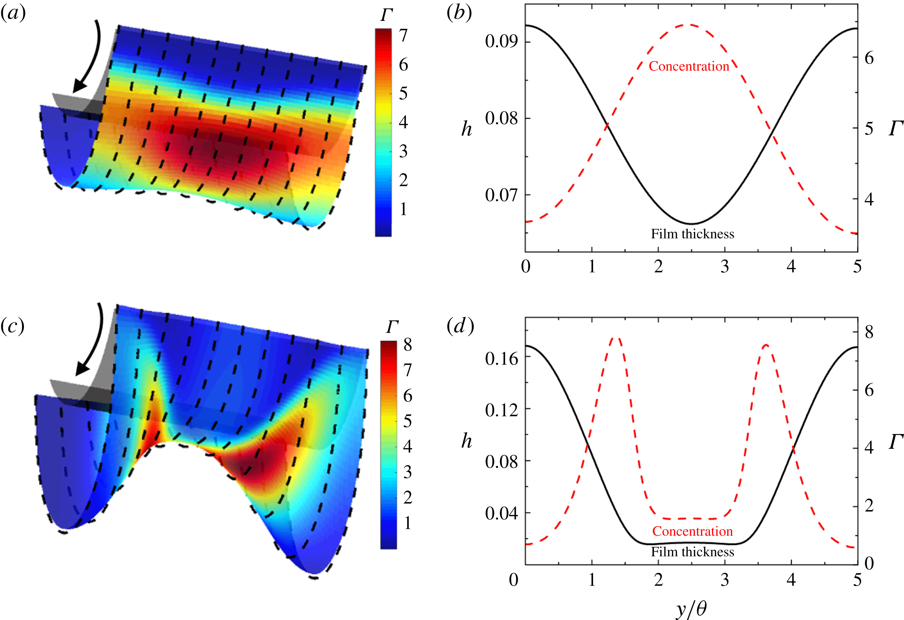
, the time evolution of surfactant concentration follows three distinct stages. We show in figures 8 and 9 the corresponding free-surface profiles and concentration distributions on the downward-moving side of the cylinder, where the surfactant concentration reaches its maximum.
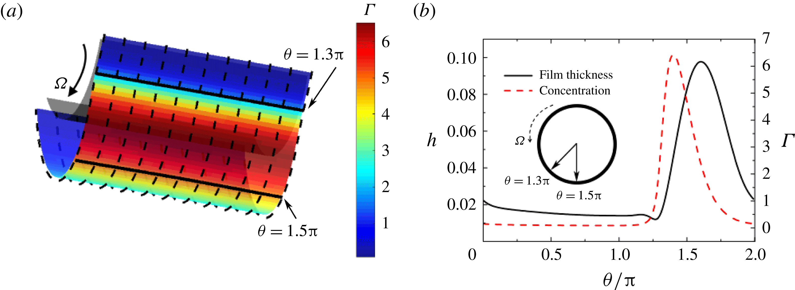
(a,c) Free-surface and concentration profiles, and film thickness (black solid lines in (b,d)) and concentration (red dashed lines in (b,d)) at
 $\unicode[STIX]{x1D703}=1.5\unicode[STIX]{x03C0}$
with
 $Bo=1$
,
 $h_{0}=0.03162$
,
 $M=0.007$
,
 $Ma=0$
,
 $Pe=10^{5}$
,
 $L=5\unicode[STIX]{x03C0}$
and
 $W=0.1$
at (a,b)
 $t=2\times 10^{6}$
and (c,d)
 $t=4\times 10^{6}$
. For ease of visualization, the thickness plotted in (a,c) is five times larger than the actual value.

Due to the initial gravity-driven drainage, surfactant tends to accumulate at the bottom of the cylinder in a liquid ridge with little concentration variation in the axial direction (red region in figure 8
a). The corresponding film thickness and concentration at
 $y=0$
are shown in figure 8(b). Surfactant concentration increases significantly on the downward-moving side of the ridge (
 $1.3\unicode[STIX]{x03C0}<\unicode[STIX]{x1D703}<1.5\unicode[STIX]{x03C0}$
), and reaches its maximum several degrees below the point of maximum thickness.
As axial perturbations start to grow in amplitude (figure 9
a), axial variations in both film thickness and surfactant concentration become significant, so we plot in figure 9(b) the film thickness and concentration along the cylinder axis at
 $\unicode[STIX]{x1D703}=1.5\unicode[STIX]{x03C0}$
(marked in figure 8
a). Figure 9(b) shows that film thickness and surface concentration evolve out of phase: liquid is driven to the ends of the cylinder forming two half-droplets at
 $y=0$
and
 $y=5\unicode[STIX]{x03C0}$
, while surfactant is driven to the middle of the cylinder, giving rise to a high-concentration region in the thin-film area (
 $y=2.5\unicode[STIX]{x03C0}$
). This happens because the region of high surfactant concentration in figure 8(a) (
 $1.3\unicode[STIX]{x03C0}<\unicode[STIX]{x1D703}<1.5\unicode[STIX]{x03C0}$
) occurs where the axial flux drives liquid to the middle of the cylinder (similar to the case shown in figure 5). As in § 5.1, the negative axial flux arises because the contribution from surface tension is stronger than the contribution from gravity and centrifugal forces. Again, the term
 $(h_{\unicode[STIX]{x1D703}\unicode[STIX]{x1D703}})_{y}$
dominates the surface-tension contribution.
The steady free-surface and concentration profiles are shown in figure 9(c). The corresponding film thickness and concentration at
 $y=1.5\unicode[STIX]{x03C0}$
are shown in figure 9(d). As the two half-droplets grow in size, a satellite droplet forms in the middle of the cylinder (small bump in between
 $2\unicode[STIX]{x03C0}<y<3\unicode[STIX]{x03C0}$
in figure 9
d). This triggers an additional capillary flow that drives surfactant away from the middle of the cylinder. As a result, the surfactant concentration in the middle of the cylinder decreases dramatically and forms maxima in between the main droplets and the satellite droplet.
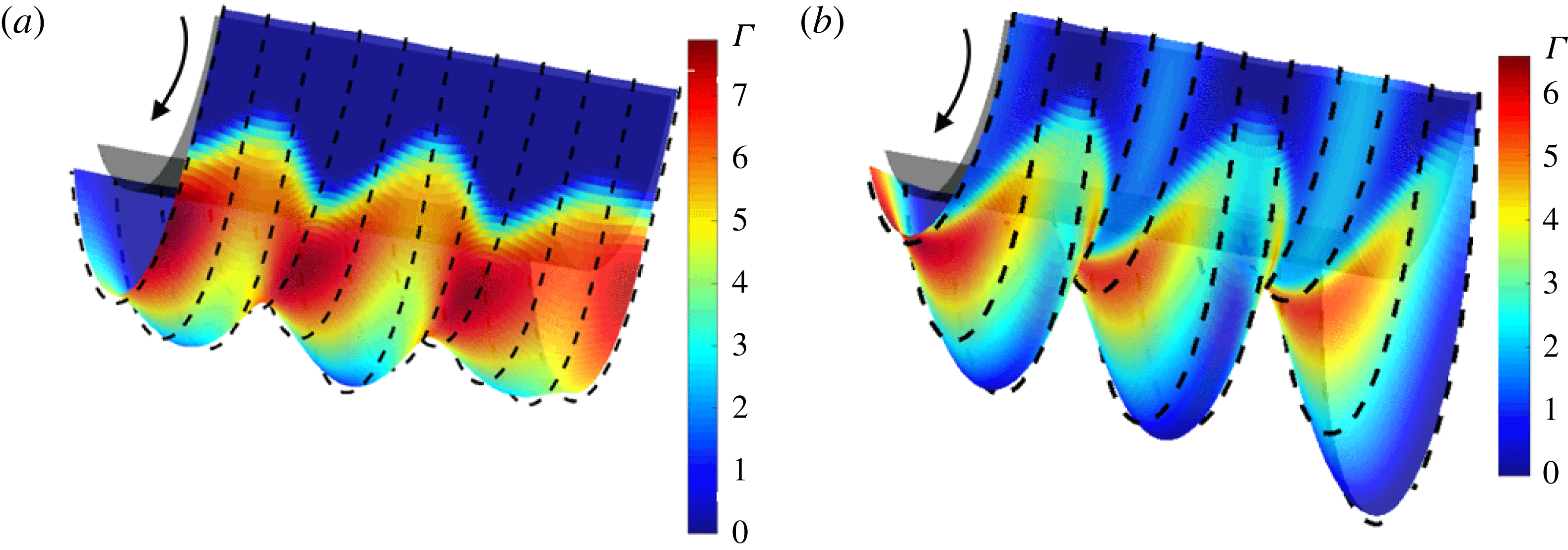
Free-surface and surfactant concentration profiles with
 $Bo=1$
,
 $h_{0}=0.03162$
,
 $L=5\unicode[STIX]{x03C0}$
,
 $M=0.007$
,
 $Ma=0.001$
,
 $Pe=10^{5}$
and
 $W=0.1$
at (a)
 $t=8.5\times 10^{4}$
(b)
 $t=2.5\times 10^{5}$
(steady state). For ease of visualization, the thickness plotted in this figure is five times larger than the actual value.

6.1.2 Marangoni stresses
We now include the influence of Marangoni stresses by performing simulations with
 $Ma=0.001$
. Figure 10(a,b) shows the free-surface and surfactant concentration profiles on the downward-moving side of the cylinder during the transient stage and at steady state, respectively. Notably, a third droplet forms in the middle of the cylinder during the transient stage, corresponding to a decrease in the spacing between droplets relative to the zero-
 $Ma$
case (figure 9
c). The third droplet grows in size together with the two half-droplets at two ends. The decrease in the spacing between droplets when
 $Ma\neq 0$
is consistent with the decrease in the cutoff wavelength in the RT regime shown in figure 4.
The results shown in figure 9 can be used to understand the growth of the third droplet. The accumulation of surfactant in between the two main droplets (figure 9 b) lowers the local surface tension, and the resulting Marangoni stresses then drive liquid away from that area to those droplets. The surfactant concentration in the middle of the cylinder becomes especially low when the satellite droplet forms (figure 9 d). The resulting Marangoni stresses then drive flow to the middle of the cylinder, leading to the formation of a third droplet (figure 10). The flows driven by the Marangoni stresses enhance the growth rate of the droplets, so steady state is reached sooner.
The Marangoni flows also lead to disappearance of the stable speed window (figure 4). Recall that the term
 $(h_{\unicode[STIX]{x1D703}\unicode[STIX]{x1D703}})_{y}$
drives flow to the middle of the cylinder and thus opposes the RT instability, leading to the large increase in the cutoff wavelength as the rotation rate is increased (figure 4
a). The Marangoni stresses initially drive flow towards the ends of the cylinder and thus oppose the flow driven by the
 $(h_{\unicode[STIX]{x1D703}\unicode[STIX]{x1D703}})_{y}$
term. As a consequence, this term becomes much less effective at opposing the RT instability and the stable speed window disappears (figure 4
b).
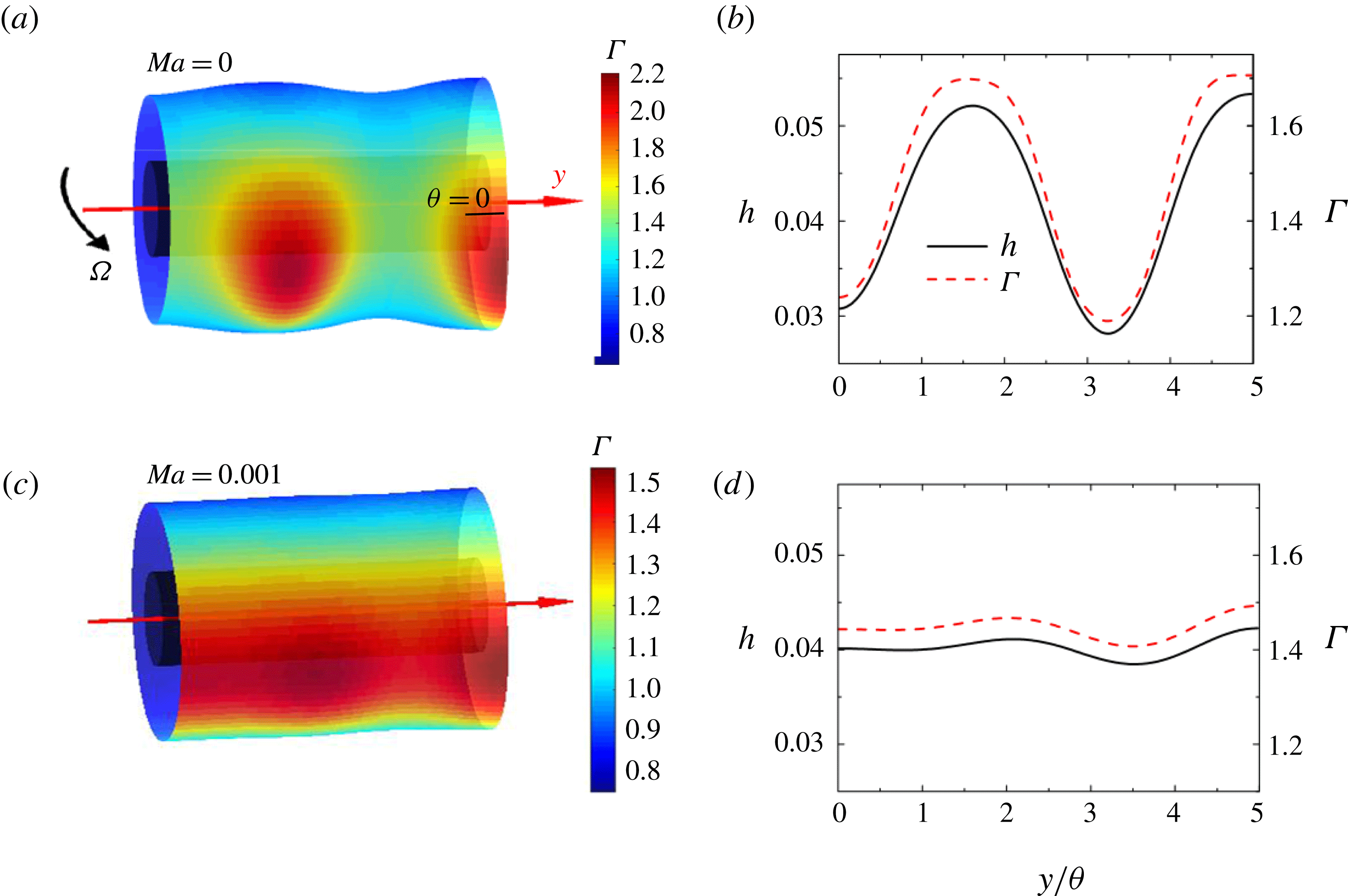
(a,c) Free-surface and surfactant concentration profiles for two different values of
 $Ma$
with
 $Bo=1$
,
 $h_{0}=0.03162$
,
 $L=5\unicode[STIX]{x03C0}$
,
 $M=0.007$
,
 $Pe=10^{5}$
and
 $W=0.3$
at
 $t=4\times 10^{6}$
. For ease of visualization, the thickness plotted in (a,c) is
 $50$
times larger than the actual value. (b,d) Corresponding film thickness (black solid lines) and concentration (red dashed lines) at
 $\unicode[STIX]{x1D703}=0$
(marked in a).

6.2 Rayleigh–Plateau instability
In the regime where the RP instability dominates (right side of figure 4
b), we again choose a representative rotation rate of
 $W=0.1$
. Figure 11(a) shows the free-surface and surfactant concentration profiles for the simulation shown in figure 7 where
 $Ma=0$
. The corresponding film thickness and surfactant concentration along the cylinder axis at
 $\unicode[STIX]{x1D703}=0$
are shown in figure 11(b). The case where
 $Ma=0.001$
is also considered, and results are shown in figure 11(c,d) for comparison.
For
 $Ma=0$
, the liquid film breaks into one-and-a-half rings wrapped circumferentially around the cylinder due to the RP instability (figure 11
a). Surfactant tends to accumulate on the upward-moving side of the rings (red regions in figure 11
a). Recall that when the rotation rate is smaller, surfactant tends to accumulate in a liquid ridge at the cylinder bottom (figure 8). As the rotation rate is increased, the ridge and point of maximum concentration shift to the upward-moving side of the cylinder (Li & Kumar Reference Li and Kumar2015). As the ridge breaks up due to the RP instability, liquid and surfactant get driven into the rings, and as a consequence, the film thickness and surfactant concentration are in phase at
 $\unicode[STIX]{x1D703}=0$
, which is on the upward-moving side (figure 11
b).
For
 $Ma=0.001$
, the gradients in film thickness and surfactant concentration are much smaller than those when
 $Ma=0$
and the coating stays almost axially uniform (figures 11
c and 11
d). Since surfactant tends to accumulate at the surface of the rings, the resulting Marangoni stresses drive flow from the rings to the thin-film areas, leading to the more uniform coating and concentration profile. In addition, these Marangoni flows slow the growth of the instability but do not appear to change the spacing between the rings.
The Marangoni flows again lead to disappearance of the stable speed window (figure 4). Recall that the term
 $(h_{\unicode[STIX]{x1D703}\unicode[STIX]{x1D703}})_{y}$
drives flow to the middle of the cylinder and thus opposes the RP instability (§ 5.2), leading to the large increase in the cutoff wavelength as the rotation rate is decreased (figure 4
a). Because the Marangoni flows lead to a smoother free surface, the
 $(h_{\unicode[STIX]{x1D703}\unicode[STIX]{x1D703}})_{y}$
term is much less effective at opposing the RP instability and the stable speed window disappears (figure 4
b).
7 Flow visualization experiments
To complement our numerical simulations, we have performed some flow visualization experiments. We first describe the experimental set-up, and then present and discuss the results.
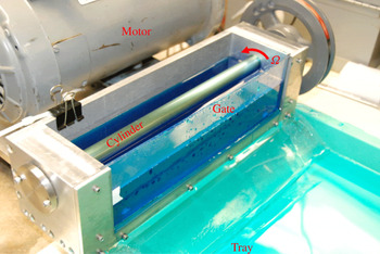
7.1 Experimental set-up
The experimental apparatus is shown in figure 12. A smooth steel cylinder is mounted in a container whose front gate can be lifted, and the cylinder is rotated using an electric motor. In all of our experiments, liquid was first coated on the cylinder by rotating it with the container partially filled. The glass gate was then quickly lifted to drain the liquid from the container into a tray, leaving liquid on the rotating cylinder. Excess liquid would immediately drip off, which sometimes triggered visible axial variations in coating thickness or even dry patches. As a result, we sometimes had to repeat this process until a sufficiently uniform initial coating was obtained.
The steel cylinder has radius
 $R=0.2~\text{cm}$
, which is consistent with the value used in our simulations (table 1), and length
 $L=30~\text{cm}$
. The liquid is a glycerol/water mixture (96 wt % glycerol) having surface tension
 $\unicode[STIX]{x1D70E}_{0}=66~\text{dyn}~~\text{cm}^{-1}$
, density
 $\unicode[STIX]{x1D70C}=1.23~\text{g}~\text{cm}^{-3}$
and viscosity
 $\unicode[STIX]{x1D707}=2.6~\text{P}$
. To study the influence of surfactant, we use sodium dodecyl sulphate (SDS; Thermo Scientific). For a bulk concentration
 $c=0.1$
wt %, the surface tension drops to
 $50~\text{dyn}~~\text{cm}^{-1}$
, while the density and viscosity remain unchanged. An increase in
 $c$
further reduces surface tension, suggesting that
 $c=0.1~\text{wt}\%$
is still smaller than the critical micelle concentration.
The values of key dimensionless parameters in the experiments are summarized in table 3. Note that
 $Bo$
in our experiments is around unity, consistent with the simulations. The dimensionless viscosity in our experiments (
 $M=0.74$
) is approximately 100 times higher than that in our simulations (
 $M=0.007$
) so that a much thicker coating can be maintained on the cylinder for ease of flow visualization. As noted in § 4, if
 $M$
or the initial film thickness are too large, a stable speed window may not be observed. In the experiments, the smallest rotation rates (
 $W\sim 0.03{-}0.06$
) were comparable to those in the simulations, while the largest rotation rates (
 $W\sim 0.2{-}0.3$
) were smaller. The Marangoni number in our experiments (
 $Ma=0.35$
) is much larger than that in our simulations (
 $Ma=0.001$
), so we expect to observe much stronger Marangoni effects in the experiments.
Experimental apparatus. The steel cylinder has length
 $L=30~\text{cm}$
and radius
 $R=0.2~\text{cm}$
.

Dimensionless problem parameters.

7.2 Results and discussion
For the surfactant-free solution (which corresponds to
 $Ma=0$
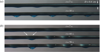
), images of the free surface on the upward-moving side of the cylinder at several different times are shown in figure 13 for
 $W=0.056$
and
 $W=0.22$
.
Images of the free surface on the upward-moving side of the cylinder for the surfactant-free solution at several different times for (a)
 $W=0.056$
and (b)
 $W=0.22$
with
 $Bo=0.73$
,
 $M=0.74$
and
 $Ma=0$
.

For
 $W=0.056$
(figure 13
a), axial perturbations grow in amplitude due to gravity, and become visible near the underside of the cylinder within approximately 7 s (1 s corresponds to approximately 100 dimensionless time units). At later times, the coating breaks up into small droplets which are approximately evenly spaced along the cylinder axis, similar to the simulation result shown in figure 5 for the Rayleigh–Taylor instability. The sizes of the droplets reach a steady state within about 35 s, with the droplets tending to slowly shift along the cylinder axis.
With an increase in rotation rate to
 $W=0.22$
, there is a transition from the Rayleigh–Taylor instability to the Rayleigh–Plateau instability (figure 13
b). Initial perturbations grow into small ring-shaped liquid bulges under the action of centrifugal forces, similar to the simulation result shown in figure 7 for the Rayleigh–Plateau instability. These bulges are not stable, and adjacent ones tend to merge to form a droplet (marked by arrows in figure 13
b). We do observe some shifting of rings along the cylinder axis in our simulations (§ 5.2), but are not able to run simulations for a long enough time to observe merging. The formation of large bulges enhances the strength of gravitational forces and appears to draw liquid from the surrounding areas, which leads to a droplet. The sizes of the rings and droplet reach a steady state at a later time (
 ${\sim}$
70 s) compared to the low rotation rate case (figure 13
a).
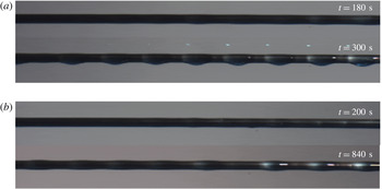
Images of the free surface on the upward-moving side of the cylinder for the surfactant-laden solution at several different times for (a)
 $W=0.056$
and (b)
 $W=0.22$
with
 $Bo=1.0$
,
 $M=0.74$
and
 $Ma=0.35$
.

For the surfactant-laden solution (which corresponds to
 $Ma=0.35$
), images of the free surface on the upward-moving side of the cylinder at several different times are shown in figure 14 for
 $W=0.056$
and
 $W=0.22$
. Similar to the surfactant-free case, droplets form at the lower rotation rate (figure 14
a) while rings form at the higher rotation rate (figure 14
b). However, the time required for axial perturbations to become visible is much longer compared to the surfactant-free case for both rotation rates. As a consequence, the sizes of the droplets and rings reach steady state at much later times,
 ${\sim}5$
min. for the droplets and
 ${\sim}10$
min. for the rings. In addition, the shifting and merging of rings and droplets seen in the surfactant-free case (figure 13
b) appears to be considerably suppressed when surfactant is present.
The slower development of free-surface perturbations at the higher rotation rate when
 $Ma\neq 0$
is consistent with the simulation results in § 6.2 for the RP instability. However, the simulation results for the RT instability in § 6.2 predict a faster development of free-surface perturbations when
 $Ma\neq 0$
, in contrast to the experimental observations at the lower rotation rate. We believe that this situation arises because the initial coating in the experiments is non-axisymmetric, in contrast to the initial condition used in the simulations. The non-axisymmetric initial condition in the experiments arises due to liquid dripping. When surfactant is present, the resulting Marangoni stresses tend to suppress this dripping (Weidner Reference Weidner2013), leading to a slower development of free-surface perturbations. Nevertheless, this slower development created by surfactant may be very useful for applications, allowing for a longer time period to solidify the coating before free-surface perturbations become prominent.
Most dangerous wavelength at different rotation rates with
 $M=0.74$
and (a)
 $Bo=0.73$
and
 $Ma=0$
and (b)
 $Bo=1.0$
and
 $Ma=0.35$
. Red dashed lines and blue solid lines indicate the most dangerous wavelength obtained from linear stability analysis.

We have also measured the average spacing between the free-surface bulges as soon as they become visible over a range of rotation rates (figure 15). This spacing should correspond the most dangerous wavelength, and is shown in non-dimensional form (scaled with
 $R$
) in figure 15. Each point in figure 15 represents a mean of up to four measurements. For the surfactant-free solution, the largest deviation from the mean value of the most dangerous wavelength was
 $0.3\unicode[STIX]{x03C0}$
, whereas for the surfactant-free solution, the largest deviation from the mean was much smaller,
 $0.05\unicode[STIX]{x03C0}$
, presumably due to the reduced shifting and merging of rings and droplets. Also shown in figure 15 are predictions of the most dangerous wavelength from LSA for the RT and RP instabilities (see supplementary material and § 4), yielding plots similar to those for the cutoff wavelength shown in figure 4.
The most dangerous wavelengths of the RT and RP instabilities in the surfactant-free case are (Evans et al. Reference Evans, Schwartz and Roy2005)
 $$\begin{eqnarray}\text{RT instability:}\quad \unicode[STIX]{x1D706}_{drop}^{\star }=\frac{2\sqrt{2}\unicode[STIX]{x03C0}}{\sqrt{Bo}},\quad \text{RP instability:}\quad \unicode[STIX]{x1D706}_{ring}^{\star }=\frac{2\sqrt{2}\unicode[STIX]{x03C0}}{1+S},\end{eqnarray}$$
where
 $S=WBo^{2}$
is the Weber number defined in § 3. When
 $Ma\neq 0$
, analytical expressions for these quantities are not available, but calculations show that surfactant has only a very minor influence (see supplementary material). We thus use the expressions given in (7.1a,b
) even when
 $Ma\neq 0$
, similar to figure 4.
For the surfactant-free solution (figure 15
a), the average spacing oscillates about
 $\unicode[STIX]{x1D706}_{drop}^{\star }$
(red dotted line) at low rotation rates, and is always larger than
 $\unicode[STIX]{x1D706}_{ring}^{\star }$
(blue solid line) at high rotation rates. The discrepancy at high rotation rates is consistent with the merging of the rings (figure 14
b), which lowers the number of rings along cylinder axis and causes the average spacing to increase. No stable speed window is observed, perhaps due to the large value of
 $M$
and a relatively thick and non-uniform initial film.
For the surfactant-laden solution, (figure 15
b), the average spacing is generally smaller compared to the surfactant-free case. This is consistent with the observation that surfactant lowers the mean surface tension,
 $\unicode[STIX]{x1D70E}_{m}$
(larger
 $Bo$
), which gives rise to a larger value of
 $Bo$
and a smaller value of the most dangerous wavelength (7.1a,b
). Again, no stable speed window is observed over the range of rotation rates considered.
When
 $W=0.028$
, the average spacing measured in our experiments is
 $\unicode[STIX]{x1D706}/\unicode[STIX]{x03C0}=2.0$
(
 ${\sim}0.4$
cm) in the surfactant-laden solution, which is much smaller than
 $\unicode[STIX]{x1D706}_{drop}^{\star }/\unicode[STIX]{x03C0}=2.8$
calculated using LSA (red dotted line in figure 15
b). With an increase in
 $W$
, the average spacing increases monotonically in the RT-instability regime and reaches its maximum at
 $W=0.12$
. The discrepancy between the experimental values and the LSA predictions is consistent with our simulation results, which show that Marangoni stresses lead to the formation of extra droplets along the cylinder axis (figure 10), which would cause the average spacing to be smaller than that predicted by the simple RT LSA result. An increase in the rotation rate weakens the effects of gravity, and as a result, the coating becomes more stable to the RT instability. This explains the increase in the average spacing with increasing
 $W$
in the regime of the RT instability.
A further increase in
 $W$
brings the system into the regime of the RP instability. Here, the average spacing decreases as the rotation rate increases, and there is much better agreement between the experimental observations and the LSA predictions relative to the RT regime (blue solid line in figure 15
b). This can be rationalized by recalling that Marangoni stresses suppress the growth rate of the RP instability but do not modify the spacing between rings (§ 6.2). The behaviour of the most dangerous wavelength shown in figure 15(b) is analogous to the behaviour of the cutoff wavelength shown in figure 4(b), where the cutoff wavelength from the simulations is smaller than the LSA prediction at low rotation rates, but in much better agreement at high rotation rates.
We have also attempted to perform some nonlinear simulations to predict the most dangerous wavelength using an initial film thickness estimated from (1.1) and experimental observations of
 $\unicode[STIX]{x1D6FA}_{c}$
. However, since the initial film thickness is much larger than that used for the simulations in §§ 4–6, large free-surface deformations quickly develop that we cannot accurately resolve, and as a consequence, we are unable to obtain predictions of the most dangerous wavelength from the simulations. The same issue arises if we try to use a non-axisymmetric initial condition similar to that in the experiments.
Nevertheless, the results of these flow visualization experiments appear to be qualitatively consistent with predictions from LSA and other behaviour observed in our simulations. We note that while the simulations and LSA are for the case of an insoluble surfactant, the surfactant in the experiments is soluble. Nevertheless, it appears that much of what is observed in the experiments can largely be understood by a model that assumes surfactant insolubility, suggesting that surfactant solubility plays a secondary role in these experiments.
8 Conclusions
One purpose of this paper was to determine the physical mechanisms underlying the stable speed window observed by Evans et al. (Reference Evans, Schwartz and Roy2005). Our simulations show that surface-tension forces arising from both axial and angular variations in the angular curvature drive flows in the axial direction that tend to smooth out free-surface perturbations. The term responsible for this,
 $(h_{\unicode[STIX]{x1D703}\unicode[STIX]{x1D703}})_{y}$
, is not present in the standard axisymmetric RP instability or in the RT instability for a film under a planar substrate.
A second purpose of this paper was to determine how the presence of insoluble surfactant influences three-dimensional thin liquid film flow on rotating cylinders. Our simulations show that Marangoni stresses can cause the stable speed window to disappear by driving flows that oppose those arising from the
 $(h_{\unicode[STIX]{x1D703}\unicode[STIX]{x1D703}})_{y}$
term. In addition, Marangoni stresses tend to reduce the spacing between droplets at low rotation rates (RT-instability regime), and reduce the growth rate of the rings at high rotation rates (RP-instability regime). Our results extend those of (i) Weidner (Reference Weidner2013) to include cylinder rotation, (ii) Evans et al. (Reference Evans, Schwartz and Roy2005) to include insoluble surfactant and (iii) Li & Kumar (Reference Li and Kumar2015) to include axial variations.
Flow visualization experiments yield observations that are qualitatively consistent with LSA predictions and behaviour observed in the simulations. Although a stable speed window was not observed, the flow visualizations make clear that surfactants tend to suppress dripping, slow the development of free-surface perturbations and reduce the shifting and merging of rings and droplets. This may be very useful for applications as it would allow a longer time period to solidify the coating before free-surface perturbations become too large.
While some of the results presented here can readily be understood in terms of the RT and RP instabilities, others appear to arise as a consequence of cylinder rotation. Many objects that need to be coated have a more complex cross-sectional shape, resulting in additional flows that arise due to curvature gradients on the object surface (Li, Carvalho & Kumar Reference Li, Carvalho and Kumar2017b ). Nevertheless, the results obtained for the model problem considered here may be useful in understanding many features of the even more complex flows likely to arise is those cases.
Acknowledgements
This work was supported through the Industrial Partnership for Research in Interfacial and Materials Engineering of the University of Minnesota. We are grateful to the Minnesota Supercomputing Institute (MSI) at the University of Minnesota for providing computational resources. We thank W. Suszynski for assistance with the experiments and L. Espín for helpful discussions.
Supplementary materials
Supplementary materials are available at https://doi.org/10.1017/jfm.2018.153.
Appendix A. Derivation of evolution equations
We summarize here the derivation of the evolution equations (2.11) and (2.12). After introducing the scalings (2.10), governing equations (2.3) and (2.4) become (tildes dropped)
 $$\begin{eqnarray}\displaystyle & \displaystyle \frac{\unicode[STIX]{x2202}}{\unicode[STIX]{x2202}z}(rw)+\frac{\unicode[STIX]{x2202}u}{\unicode[STIX]{x2202}\unicode[STIX]{x1D703}}+r\frac{\unicode[STIX]{x2202}v}{\unicode[STIX]{x2202}y}=0, & \displaystyle\end{eqnarray}$$
 $$\begin{eqnarray}\displaystyle & \displaystyle -W^{2}(1+\unicode[STIX]{x1D716}z)=-\frac{\unicode[STIX]{x2202}p}{\unicode[STIX]{x2202}z}+\unicode[STIX]{x1D716}\frac{\unicode[STIX]{x2202}^{2}w}{\unicode[STIX]{x2202}^{2}z}-\sin \unicode[STIX]{x1D703}, & \displaystyle\end{eqnarray}$$
 $$\begin{eqnarray}\displaystyle & \displaystyle 0=-\unicode[STIX]{x1D716}\frac{\unicode[STIX]{x2202}p}{\unicode[STIX]{x2202}\unicode[STIX]{x1D703}}+\frac{\unicode[STIX]{x2202}^{2}u}{\unicode[STIX]{x2202}^{2}z}+\unicode[STIX]{x1D716}\frac{\unicode[STIX]{x2202}u}{\unicode[STIX]{x2202}z}-\cos \unicode[STIX]{x1D703}, & \displaystyle\end{eqnarray}$$
 $$\begin{eqnarray}\displaystyle & \displaystyle 0=-\unicode[STIX]{x1D716}\frac{\unicode[STIX]{x2202}p}{\unicode[STIX]{x2202}y}+\left(\frac{\unicode[STIX]{x2202}^{2}}{\unicode[STIX]{x2202}z^{2}}+\unicode[STIX]{x1D716}\frac{\unicode[STIX]{x2202}}{\unicode[STIX]{x2202}z}\right)v, & \displaystyle\end{eqnarray}$$
where
 $W=\unicode[STIX]{x1D6FA}/\sqrt{g/R}$
is the dimensionless rotation rate. Note that terms of
 $O(\unicode[STIX]{x1D716}^{2})$
are neglected in the above equations and those below. As a consequence, the Reynolds numbers
 $Re=\unicode[STIX]{x1D70C}^{2}gH^{2}R/\unicode[STIX]{x1D707}^{2}$
and
 $Re_{\unicode[STIX]{x1D6FA}}=\unicode[STIX]{x1D70C}\unicode[STIX]{x1D6FA}R^{2}/\unicode[STIX]{x1D707}$
can be no larger than
 $O(1)$
(Evans et al.
Reference Evans, Schwartz and Roy2004, Reference Evans, Schwartz and Roy2005).
The simplified tangential stress boundary conditions in
 $\unicode[STIX]{x1D703}$
- and
 $y$
-directions are
 $$\begin{eqnarray}\displaystyle & \displaystyle \frac{\unicode[STIX]{x2202}u}{\unicode[STIX]{x2202}z}-\unicode[STIX]{x1D716}u=\unicode[STIX]{x1D716}Ma\frac{\unicode[STIX]{x2202}\unicode[STIX]{x1D70E}}{\unicode[STIX]{x2202}\unicode[STIX]{x1D703}}, & \displaystyle\end{eqnarray}$$
 $$\begin{eqnarray}\displaystyle & \displaystyle \frac{\unicode[STIX]{x2202}v}{\unicode[STIX]{x2202}z}=\unicode[STIX]{x1D716}Ma\frac{\unicode[STIX]{x2202}\unicode[STIX]{x1D70E}}{\unicode[STIX]{x2202}y}, & \displaystyle\end{eqnarray}$$
where the Marangoni number
 $Ma=\unicode[STIX]{x1D711}/\unicode[STIX]{x1D707}U$
measures the strength of surface-tension-gradient forces relative to viscous forces. For dilute concentrations of surfactant such that
 $\unicode[STIX]{x1D711}/\unicode[STIX]{x1D70E}_{m}\sim \unicode[STIX]{x1D716}$
, the normal stress boundary condition (2.6) becomes
 $$\begin{eqnarray}-p+2\unicode[STIX]{x1D716}(\boldsymbol{n}\boldsymbol{\cdot }\unicode[STIX]{x1D749}\boldsymbol{\cdot }\boldsymbol{n})=-\frac{1}{\unicode[STIX]{x1D716}Bo}\unicode[STIX]{x1D705}+\unicode[STIX]{x1D716}Ma\unicode[STIX]{x1D70E}.\end{eqnarray}$$
The Bond number,
 $Bo=\unicode[STIX]{x1D70C}gR^{2}/\unicode[STIX]{x1D70E}_{m}$
, measures the importance of surface-tension forces relative to gravitational forces. The outward unit normal
 $\boldsymbol{n}$
, surface curvature
 $\unicode[STIX]{x1D705}$
, and rate-of-strain tensor
 $\unicode[STIX]{x1D749}$
(non-dimensionalized by
 $U/R$
) are given by
 $$\begin{eqnarray}\displaystyle & \displaystyle \boldsymbol{n}=\boldsymbol{e}_{r}-\boldsymbol{e}_{\unicode[STIX]{x1D703}}\frac{\unicode[STIX]{x1D716}}{r}\frac{\unicode[STIX]{x2202}h}{\unicode[STIX]{x2202}\unicode[STIX]{x1D703}}-\boldsymbol{e}_{y}\frac{\unicode[STIX]{x2202}h}{\unicode[STIX]{x2202}y}, & \displaystyle\end{eqnarray}$$
 $$\begin{eqnarray}\displaystyle & \displaystyle \unicode[STIX]{x1D705}=1-\unicode[STIX]{x1D716}h-\unicode[STIX]{x1D716}\overline{\unicode[STIX]{x1D6FB}}^{2}h, & \displaystyle\end{eqnarray}$$
 $$\begin{eqnarray}\displaystyle & \displaystyle \unicode[STIX]{x1D70F}_{rr}=\frac{\unicode[STIX]{x2202}w}{\unicode[STIX]{x2202}z}, & \displaystyle\end{eqnarray}$$
 $$\begin{eqnarray}\displaystyle & \displaystyle \unicode[STIX]{x1D70F}_{\unicode[STIX]{x1D703}\unicode[STIX]{x1D703}}=\frac{1}{r}\frac{\unicode[STIX]{x2202}u}{\unicode[STIX]{x2202}\unicode[STIX]{x1D703}}+\unicode[STIX]{x1D716}\frac{w}{r}, & \displaystyle\end{eqnarray}$$
 $$\begin{eqnarray}\displaystyle & \displaystyle \unicode[STIX]{x1D70F}_{yy}=\frac{\unicode[STIX]{x2202}v}{\unicode[STIX]{x2202}y} & \displaystyle\end{eqnarray}$$
 $$\begin{eqnarray}\displaystyle & \displaystyle 2\unicode[STIX]{x1D70F}_{r\unicode[STIX]{x1D703}}=2\unicode[STIX]{x1D70F}_{\unicode[STIX]{x1D703}r}=\frac{1}{\unicode[STIX]{x1D716}}\frac{\unicode[STIX]{x2202}u}{\unicode[STIX]{x2202}z}-\frac{u}{r}+\frac{\unicode[STIX]{x1D716}}{r}\frac{\unicode[STIX]{x2202}w}{\unicode[STIX]{x2202}\unicode[STIX]{x1D703}}, & \displaystyle\end{eqnarray}$$
 $$\begin{eqnarray}\displaystyle & \displaystyle 2\unicode[STIX]{x1D70F}_{\unicode[STIX]{x1D703}y}=2\unicode[STIX]{x1D70F}_{y\unicode[STIX]{x1D703}}=\frac{1}{r}\frac{\unicode[STIX]{x2202}v}{\unicode[STIX]{x2202}\unicode[STIX]{x1D703}}+\frac{\unicode[STIX]{x2202}u}{\unicode[STIX]{x2202}y} & \displaystyle\end{eqnarray}$$
 $$\begin{eqnarray}\displaystyle & \displaystyle 2\unicode[STIX]{x1D70F}_{yr}=2\unicode[STIX]{x1D70F}_{ry}=\frac{1}{\unicode[STIX]{x1D716}}\frac{\unicode[STIX]{x2202}v}{\unicode[STIX]{x2202}z}+\unicode[STIX]{x1D716}\frac{\unicode[STIX]{x2202}w}{\unicode[STIX]{x2202}y}, & \displaystyle\end{eqnarray}$$
where
 $\overline{\unicode[STIX]{x1D6FB}}^{2}=\unicode[STIX]{x2202}^{2}/\unicode[STIX]{x2202}\unicode[STIX]{x1D703}^{2}+\unicode[STIX]{x2202}^{2}/\unicode[STIX]{x2202}y^{2}$
.
At the free surface, the kinematic condition (2.8) takes the form
 $$\begin{eqnarray}\frac{\unicode[STIX]{x2202}h}{\unicode[STIX]{x2202}t}+\frac{r\unicode[STIX]{x1D6FA}+u}{r}\frac{\unicode[STIX]{x2202}h}{\unicode[STIX]{x2202}\unicode[STIX]{x1D703}}+v\frac{\unicode[STIX]{x2202}h}{\unicode[STIX]{x2202}y}-w=0.\end{eqnarray}$$
At the cylinder surface, the dimensionless no-slip and no-penetration boundary conditions are
 $$\begin{eqnarray}u=w=v=0,\end{eqnarray}$$
where
 $u$
,
 $v$
and
 $w$
are velocity components defined in (2.1).
Following the works of Evans et al. (Reference Evans, Schwartz and Roy2004), Evans et al. (Reference Evans, Schwartz and Roy2005) and Li & Kumar (Reference Li and Kumar2015), we apply a perturbation expansion in the small parameter
 $\unicode[STIX]{x1D716}=H/R\ll 1$
to solve (A 1)–(A 4) subject to boundary conditions (A 5)–(A 7) and (A 16)–(A 17). The variables are expanded in powers of
 $\unicode[STIX]{x1D716}$
as
 $$\begin{eqnarray}\left.\begin{array}{@{}c@{}}\displaystyle u=u^{(0)}+\unicode[STIX]{x1D716}u^{(1)}+\ldots ,\\ \displaystyle w=w^{(0)}+\unicode[STIX]{x1D716}w^{(1)}+\ldots ,\\ \displaystyle v=v^{(0)}+\unicode[STIX]{x1D716}v^{(1)}+\ldots ,\\ \displaystyle p=\unicode[STIX]{x1D716}^{-1}p_{0}+p^{(0)}+\unicode[STIX]{x1D716}p^{(1)}+\ldots ,\end{array}\right\}\end{eqnarray}$$
where the additional pressure
 $p_{0}=Bo^{-1}$
arises due to the film being forced to take the shape of the cylinder with curvature
 $1/R$
(Evans et al.
Reference Evans, Schwartz and Roy2004).
We substitute the above expansions into (A 1)–(A 4) and solve for the leading-order pressure and velocity components:
 $$\begin{eqnarray}\displaystyle & \displaystyle p^{(0)}=-\frac{1}{Bo}(h+\overline{\unicode[STIX]{x1D6FB}}^{2}h)+(W^{2}-\sin \unicode[STIX]{x1D703})(z-h), & \displaystyle\end{eqnarray}$$
 $$\begin{eqnarray}\displaystyle & \displaystyle u^{(0)}=\cos \unicode[STIX]{x1D703}\left({\textstyle \frac{1}{2}}z^{2}-hz\right), & \displaystyle\end{eqnarray}$$
 $$\begin{eqnarray}\displaystyle & \displaystyle w^{(0)}=\sin \unicode[STIX]{x1D703}\left(\frac{1}{6}z^{3}-\frac{1}{2}hz^{2}\right)+\frac{1}{2}\cos \unicode[STIX]{x1D703}\frac{\unicode[STIX]{x2202}h}{\unicode[STIX]{x2202}\unicode[STIX]{x1D703}}z^{2}, & \displaystyle\end{eqnarray}$$
 $$\begin{eqnarray}\displaystyle & \displaystyle v^{(0)}=0. & \displaystyle\end{eqnarray}$$
Note that gravity has no influence on the axial component of the velocity at leading order (
 $v^{(0)}=0$
), but gives rise to a parabolic profile in the angular direction due to gravity-driven drainage.
At the next order, it turns out that we only need
 $u^{(1)}$
and
 $v^{(1)}$
, which are given by
 $$\begin{eqnarray}\displaystyle & \displaystyle u^{(1)}=-\cos \unicode[STIX]{x1D703}\left(\frac{1}{3}z^{3}-hz^{2}+\frac{3}{2}h^{2}z\right)-\left[\frac{1}{Bo}\frac{\unicode[STIX]{x2202}}{\unicode[STIX]{x2202}\unicode[STIX]{x1D703}}\left(h+\overline{\unicode[STIX]{x1D6FB}}^{2}h\right)\right. & \displaystyle \nonumber\\ \displaystyle & \displaystyle \quad \left.+\,(W^{2}-\sin \unicode[STIX]{x1D703})\frac{\unicode[STIX]{x2202}h}{\unicode[STIX]{x2202}\unicode[STIX]{x1D703}}\right]\left(\frac{1}{2}z^{2}-hz^{2}\right)-Maz\frac{\unicode[STIX]{x2202}\unicode[STIX]{x1D6E4}}{\unicode[STIX]{x2202}\unicode[STIX]{x1D703}}.\quad & \displaystyle\end{eqnarray}$$
 $$\begin{eqnarray}\displaystyle & \displaystyle v^{(1)}=-\left[\frac{1}{Bo}\frac{\unicode[STIX]{x2202}}{\unicode[STIX]{x2202}y}(h+\overline{\unicode[STIX]{x1D6FB}}^{2}h)+(W^{2}-\sin \unicode[STIX]{x1D703})\frac{\unicode[STIX]{x2202}h}{\unicode[STIX]{x2202}y}\right]\left(\frac{1}{2}z^{2}-hz^{2}\right)-Maz\frac{\unicode[STIX]{x2202}\unicode[STIX]{x1D6E4}}{\unicode[STIX]{x2202}y}.\qquad & \displaystyle\end{eqnarray}$$
The Marangoni terms become significant in regions where the concentration gradients are large (large
 $\unicode[STIX]{x2202}\unicode[STIX]{x1D6E4}/\unicode[STIX]{x2202}\unicode[STIX]{x1D703}$
or
 $\unicode[STIX]{x2202}\unicode[STIX]{x1D6E4}/\unicode[STIX]{x2202}y$
), and the resulting forces drive flow from areas of high concentration to low concentration.
After integrating the continuity equation (A 1) from
 $z=0$
to
 $z=h$
and then substituting the result into (A 16), we obtain the evolution equation for the film thickness,
 $$\begin{eqnarray}\displaystyle & \displaystyle (1+\unicode[STIX]{x1D716}h)\frac{\unicode[STIX]{x2202}h}{\unicode[STIX]{x2202}t}=-\left(\frac{MW}{\unicode[STIX]{x1D716}^{2}}\right)\frac{\unicode[STIX]{x2202}}{\unicode[STIX]{x2202}\unicode[STIX]{x1D703}}\left(h+\unicode[STIX]{x1D716}\frac{h^{2}}{2}\right)+\frac{\unicode[STIX]{x2202}}{\unicode[STIX]{x2202}\unicode[STIX]{x1D703}}\left[\left(\frac{h^{3}}{3}+\unicode[STIX]{x1D716}\frac{h^{4}}{2}\right)\cos \unicode[STIX]{x1D703}\right]\qquad \qquad \qquad & \displaystyle \nonumber\\ \displaystyle & \displaystyle \qquad \quad -\,\unicode[STIX]{x1D716}\overline{\unicode[STIX]{x1D735}}\boldsymbol{\cdot }\left[\frac{h^{3}}{3Bo}\overline{\unicode[STIX]{x1D735}}(h+\overline{\unicode[STIX]{x1D6FB}}^{2}h)+\frac{h^{3}}{3}(W^{2}-\sin \unicode[STIX]{x1D703})\overline{\unicode[STIX]{x1D735}}h-\frac{1}{2}Mah^{2}\overline{\unicode[STIX]{x1D735}}\unicode[STIX]{x1D6E4}\right], & \displaystyle\end{eqnarray}$$
where
 $\overline{\unicode[STIX]{x1D735}}=\boldsymbol{e}_{\unicode[STIX]{x1D703}}(\unicode[STIX]{x2202}/\unicode[STIX]{x2202}\unicode[STIX]{x1D703})+\boldsymbol{e}_{y}(\unicode[STIX]{x2202}/\unicode[STIX]{x2202}y)$
. The first term on the right-hand side arises due to the solid-body rotation, in which
 $M=\unicode[STIX]{x1D707}/\unicode[STIX]{x1D70C}\sqrt{gR^{3}}$
is a dimensionless viscosity and
 $MW/\unicode[STIX]{x1D716}^{2}$
gives the ratio of the cylinder surface speed to the characteristic velocity. This constant is assumed to be
 $O(1)$
or smaller to ensure that surface tension plays an important role in supporting excess liquid near the underside of the cylinder. For further details of the derivation, we refer the reader to the works of Evans et al. (Reference Evans, Schwartz and Roy2004) and Evans et al. (Reference Evans, Schwartz and Roy2005).
Following the scaling and expansion procedure described above, the surfactant transport equation (2.9) becomes
 $$\begin{eqnarray}r\frac{\unicode[STIX]{x2202}\unicode[STIX]{x1D6E4}}{\unicode[STIX]{x2202}t}+\frac{\unicode[STIX]{x2202}}{\unicode[STIX]{x2202}\unicode[STIX]{x1D703}}\left(r\frac{MW}{\unicode[STIX]{x1D716}^{2}}\unicode[STIX]{x1D6E4}+u_{s}\unicode[STIX]{x1D6E4}\right)+\frac{\unicode[STIX]{x2202}}{\unicode[STIX]{x2202}y}\left[\unicode[STIX]{x1D6E4}v_{s}\right]+\unicode[STIX]{x1D716}\frac{\unicode[STIX]{x2202}h}{\unicode[STIX]{x2202}t}\unicode[STIX]{x1D6E4}=\frac{1}{Pe}\frac{\unicode[STIX]{x2202}}{\unicode[STIX]{x2202}\unicode[STIX]{x1D703}}\left(\frac{1}{r}\frac{\unicode[STIX]{x2202}\unicode[STIX]{x1D6E4}}{\unicode[STIX]{x2202}\unicode[STIX]{x1D703}}\right)+\frac{1}{Pe}\frac{\unicode[STIX]{x2202}}{\unicode[STIX]{x2202}y}\left(r\frac{\unicode[STIX]{x2202}\unicode[STIX]{x1D6E4}}{\unicode[STIX]{x2202}y}\right),\end{eqnarray}$$
where the Pélet number,
 $Pe=UR/D$
, measures the strength of surfactant convection relative to diffusion. The surface velocity,
 $(u_{s},v_{s})=(u,v)|_{z=h}$
, is given by
 $$\begin{eqnarray}\displaystyle & \displaystyle u_{s}=-\frac{1}{2}h^{2}\cos \unicode[STIX]{x1D703}-\unicode[STIX]{x1D716}\frac{5}{6}h^{3}\cos \unicode[STIX]{x1D703}-\unicode[STIX]{x1D716}Mah\frac{\unicode[STIX]{x2202}\unicode[STIX]{x1D6E4}}{\unicode[STIX]{x2202}\unicode[STIX]{x1D703}}\qquad & \displaystyle \nonumber\\ \displaystyle & \displaystyle \qquad \quad +\,\unicode[STIX]{x1D716}\frac{1}{2}\left\{\frac{h^{2}}{Bo}\frac{\unicode[STIX]{x2202}}{\unicode[STIX]{x2202}\unicode[STIX]{x1D703}}\left(h+\overline{\unicode[STIX]{x1D6FB}}^{2}h\right)+h^{2}(W^{2}-\sin \unicode[STIX]{x1D703})\frac{\unicode[STIX]{x2202}h}{\unicode[STIX]{x2202}\unicode[STIX]{x1D703}}\right\}. & \displaystyle\end{eqnarray}$$
 $$\begin{eqnarray}\displaystyle & \displaystyle v_{s}=\unicode[STIX]{x1D716}\frac{1}{2}\left\{\frac{h^{2}}{Bo}\frac{\unicode[STIX]{x2202}}{\unicode[STIX]{x2202}y}\left(h+\overline{\unicode[STIX]{x1D6FB}}^{2}h\right)+h^{2}(W^{2}-\sin \unicode[STIX]{x1D703})\frac{\unicode[STIX]{x2202}h}{\unicode[STIX]{x2202}y}\right\}-\unicode[STIX]{x1D716}Mah\frac{\unicode[STIX]{x2202}\unicode[STIX]{x1D6E4}}{\unicode[STIX]{x2202}y}. & \displaystyle\end{eqnarray}$$
Further details of the derivation can be found in the work of Weidner (Reference Weidner2013).