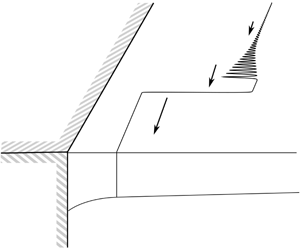

1 Introduction
Coastal or boundary currents are an integral part of global ocean circulation. For example, currents may respond to external forcing or intrinsic instability by expelling vortex filaments or larger eddies into the ocean, with implications for the mixing of coastal and ocean waters; and currents driven by outflows are important for the transport of freshwater, pollutants and land-derived nutrients. Theoretical studies of coastal currents often employ idealised models in which the current and the upper ocean have uniform potential vorticity (PV), a simplification that allows the dynamics to be understood by following the evolution of the PV front separating the ocean from the current. Stern & Pratt (Reference Stern and Pratt1985) use this model to study the nonlinear evolution of a coastal front in a non-rotating environment, Pratt & Stern (Reference Pratt and Stern1986) develop a general model for a PV front in the quasi-geostrophic (QG) limit and Grimshaw & Yi (Reference Grimshaw and Yi1990) discuss long waves on a PV front, including the effects of bottom topography. There is also much interest in the behaviour of ‘free’ fronts, i.e. those that are far from the coast, which can be used to model western boundary currents such as the Gulf Stream or the Kuroshio Extension (Pratt Reference Pratt1988; Cushman-Roisin, Pratt & Ralph Reference Cushman-Roisin, Pratt and Ralph1993; Nycander, Dritschel & Sutyrin Reference Nycander, Dritschel and Sutyrin1993; Tracey et al. Reference Tracey, Watts, Donohue and Ichikawa2012).
The present work is concerned with unforced long waves on a coastal front. We employ a  $1\frac{1}{2}$-layer, QG model introduced by Pratt & Stern (Reference Pratt and Stern1986), where the coast is a vertical boundary and the front separates two regions of constant PV. Although the model is developed in a general form by Pratt & Stern (Reference Pratt and Stern1986), their specific calculations are mostly concerned with free fronts, in which the only wave is the Rossby wave. Rossby waves are driven by vortex induction, which is a local effect acting at the front. Pratt & Stern (Reference Pratt and Stern1986) show that long waves on a free front are stationary at leading order, and at next order the curvature of the front obeys the modified Korteweg–de Vries (KdV) equation (Pratt Reference Pratt1988; Nycander et al. Reference Nycander, Dritschel and Sutyrin1993). The picture is dramatically different in the presence of a coastal boundary, and the purpose of this work is to provide an initial exploration of the regime in which the front is sufficiently close to the boundary to be influenced by two additional effects: namely Kelvin wave-driven flow and flow due to the image of the vortical current in the boundary. The Kelvin wave flow drives fluid to the right (in the northern hemisphere), while the direction of the image effect depends on the sign of the PV anomaly in the current. The combination of the two coastal effects and the Rossby wave leads to a rich set of dynamics, with the behaviour of the front depending strongly on the relative strengths of the three mechanisms. In the present model this is made explicit by introducing the non-dimensional Rossby radius, denoted
 $a$, as a key parameter (following Johnson, Southwick & McDonald Reference Johnson, Southwick and McDonald2017). When
 $a<1$ the dynamics is dominated by the Kelvin wave flow, and perturbations to the front travel faster when they are closer to the coast. However, when
 $a>1$ and the dynamics is dominated by vorticity, there is a critical off-shore distance at which perturbations travel fastest, the long-wave speed is non-monotonic and compound-wave structures are possible.
When first-order dispersive effects are included in the model, the governing equation belongs to a class of ‘weakly dispersive’ equations and is somewhat similar to the modified KdV equation. The technique of ‘dispersive shock-fitting’ developed by El (Reference El2005) can be used to analyse the initial-value problem where the initial condition consists of a step-change in frontal displacement (the Riemann problem), and to describe the propagation of dispersive shock waves (DSWs) on the front. A DSW is an expanding, slowly modulated wavetrain that connects two slowly varying far-field states, and is a generic structure in conservation laws modified by weak dispersion only (as opposed to systems modified by dispersion and dissipation). El, Grimshaw & Smyth (Reference El, Grimshaw and Smyth2006) and El, Grimshaw & Kamchatnov (Reference El, Grimshaw and Kamchatnov2007) analyse DSWs in the context of gravity waves (see also Esler & Pearce (Reference Esler and Pearce2011) for a two-layer example). The DSWs that arise from more general initial conditions may also be described using El’s technique, following Kamchatnov (Reference Kamchatnov2019).
This remainder of this work is organised as follows. Section 2 develops the mathematical model and the governing equations in the long-wave limit; §§ 3 and 4 discuss the leading-order and first-order long-wave equations, respectively, including the application of El’s technique in § 4; § 5 presents numerical results to both the long-wave and full QG equations, and considers how El’s technique can be applied to compound-wave structures; and § 6 discusses applications of the present model, and compares results with those of previous studies.
2 Mathematical formulation
A coastal current occupies the region  $0<y<Y(x,t)$. The current has uniform potential vorticity,
 $q=\unicode[STIX]{x1D6F1}$, and the ambient upper layer has uniform potential vorticity,
 $q=0$. Both the current and the upper layer lie above a deep, inactive, denser layer.

Consider flow in the half-space  $y>0$, with a vertical, impermeable wall at
 $y=0$. The flow is described by a Cartesian coordinate system
 $Oxyz$, which is fixed in a frame of reference that rotates at speed
 $f/2>0$ about the vertical axis
 $Oz$. The flow consists of an upper layer of density
 $\unicode[STIX]{x1D70C}_{1}$, lying below a rigid top at
 $z=0$ and above an inactive, infinitely deep layer of density
 $\unicode[STIX]{x1D70C}_{2}$, with
 $\unicode[STIX]{x1D70C}_{1}<\unicode[STIX]{x1D70C}_{2}$ and the difference sufficiently small that the Boussinesq approximation applies. The perturbation of the interface about the mean depth
 $H$ is denoted
 $h(x,y,t)$. A schematic of this set-up is shown in figure 1. If
 $h\ll H$, then the flow can be described by the QG equation for the conservation of potential vorticity:
 $$\begin{eqnarray}\frac{\text{D}~}{\text{D}t}\left(\unicode[STIX]{x1D6FB}^{2}\unicode[STIX]{x1D713}-\frac{1}{L_{R}^{2}}\unicode[STIX]{x1D713}\right)=0.\end{eqnarray}$$
Here,  $L_{R}=\surd (g^{\prime }H)/f$ is the Rossby radius of deformation for the upper layer,
 $g^{\prime }$ is the reduced gravity and the streamfunction
 $\unicode[STIX]{x1D713}=g^{\prime }h/f$ is related to the velocity by
 $(u,v)=(-\unicode[STIX]{x1D713}_{y},\unicode[STIX]{x1D713}_{x})$ (subscripts denote partial derivatives). The conserved quantity in (2.1) is
 $q$, the QG PV (technically
 $q$ is the perturbation PV due to the departure from the mean value
 $f/H$, multiplied by
 $H$, but as is commonplace we will refer to
 $q$ as the PV directly). In the present work
 $q$ is taken to be piecewise constant, with
 $q=\unicode[STIX]{x1D6F1}_{0}$ in the coastal current and
 $q=0$ in the ambient fluid. The front that separates the coastal current from the ambient is a material contour
 $\unicode[STIX]{x1D6E4}(t)$, knowledge of which is sufficient to determine the entire flow field at that time.
The no-flux boundary condition at  $y=0$ requires that
 $$\begin{eqnarray}\unicode[STIX]{x1D713}(x,0,t)=Q_{0}\end{eqnarray}$$
is constant, while in the far field the fluid is stationary:
 $$\begin{eqnarray}\unicode[STIX]{x1D713}\rightarrow 0\quad \text{as }y\rightarrow \infty .\end{eqnarray}$$
Thus the net flux in the upper layer is  $Q_{0}H$. If
 $Q_{0}>0$, the net flux is rightwards (facing seawards) and the interface is deeper at the coast than at infinity. This is usually the case when the coastal current is driven by a river outflow (Pimenta, Kirwan Jr & Huq Reference Pimenta, Kirwan and Huq2011; Horner-Devine, Hetland & MacDonald Reference Horner-Devine, Hetland and MacDonald2015; Johnson et al. Reference Johnson, Southwick and McDonald2017). Although in the remainder of this work we assume that
 $Q_{0}>0$, the alternative setting with a net leftward flux and a shallower interface at the coast may be obtained through the transformation
 $$\begin{eqnarray}\unicode[STIX]{x1D713}\rightarrow -\unicode[STIX]{x1D713},\quad x\rightarrow -x,\quad \unicode[STIX]{x1D6F1}\rightarrow -\unicode[STIX]{x1D6F1}.\end{eqnarray}$$
Thus the results derived below apply directly to the study of, for example, a western boundary current, in which the flow is predominantly to the left. The third possibility with  $Q_{0}=0$ is not considered here but is discussed briefly in Pratt & Stern (Reference Pratt and Stern1986). The boundary condition (2.2a) with
 $Q_{0}>0$ also represents the signature of the Kelvin wave in the QG limit. When the Rossby number is finite, the Kelvin wave propagates along the coast ahead of any frontal waves and sets the boundary condition for the vortical flow behind it (Jamshidi & Johnson Reference Jamshidi and Johnson2019). In the QG limit, the Kelvin wave travels at effectively infinite speed, setting the boundary condition (2.2a) at
 $t=0^{+}$ and for all time (Hermann, Rhines & Johnson Reference Hermann, Rhines and Johnson1989). Thus the role of the coastal Kelvin wave is to set up a steady geostrophic background flow that interacts with vortical effects. Below, for brevity, we will often refer to this simply as the ‘Kelvin wave flow’.
2.1 Scaling of horizontal lengths
As depicted in figure 1, the problem of a coastal PV front has four relevant horizontal length scales. These are:  $L_{R}$, the Rossby radius of deformation;
 $Y_{\infty }$, the mean distance of the PV front from the coast;
 $\unicode[STIX]{x1D706}$, the typical wavelength of a frontal meander; and
 $L_{V}=(Q_{0}/|\unicode[STIX]{x1D6F1}_{0}|)^{1/2}$, which is the so-called vortical length scale. The latter of these is the appropriate scaling for a current of flux
 $Q_{0}$ and relative vorticity
 $|\unicode[STIX]{x1D6F1}_{0}|$ in two-dimensional flow (Johnson & McDonald Reference Johnson and McDonald2006). The QG model used for numerical simulations below assumes that all four lengths are of order unity, while the long-wave limit in which the analysis is performed formally requires
 $$\begin{eqnarray}\unicode[STIX]{x1D706}\gg (Y_{\infty },L_{R},L_{V}),\end{eqnarray}$$
with  $Y_{\infty }$,
 $L_{R}$ and
 $L_{V}$ all of the same order. By contrast, the free-front problem considered by Pratt (Reference Pratt1988) and Nycander et al. (Reference Nycander, Dritschel and Sutyrin1993) assumes that
 $$\begin{eqnarray}Y_{\infty }\gg \unicode[STIX]{x1D706}\gg (L_{R},L_{V}).\end{eqnarray}$$
Thus the present work explores a different asymptotic regime from that considered by Pratt (Reference Pratt1988) and Nycander et al. (Reference Nycander, Dritschel and Sutyrin1993), one in which  $Y_{\infty }\sim L_{R}$ and boundary effects may be important. Some examples of PV fronts in real oceans that may fall into this regime include the flow down Barrow Canyon (Pickart et al. Reference Pickart, Weingartner, Pratt, Zimmermann and Torres2005), the Kuroshio south of Japan (Tsujino, Usui & Nakano Reference Tsujino, Usui and Nakano2006) and the Western Arctic shelfbreak jet (Spall et al. Reference Spall, Pickart, Fratantoni and Plueddemann2008). Further discussion of the oceanographic context for this work is given in § 6.
We follow Johnson et al. (Reference Johnson, Southwick and McDonald2017) and non-dimensionalise horizontal lengths on  $L_{V}$. This introduces the non-dimensional Rossby radius
 $a=L_{R}/L_{V}$, which measures the relative strengths of the Kelvin wave flow and image vorticity and plays an important role in what follows. When
 $a<1$ the flow is Kelvin wave dominated, while
 $a>1$ corresponds to vorticity-dominated flow. Further physical interpretation of
 $a$ is given in the context of a coastal outflow by Johnson et al. (Reference Johnson, Southwick and McDonald2017). The parameter
 $Q_{0}$, which represents the net flux in the upper layer, can be scaled out by replacing
 $\unicode[STIX]{x1D713}$ with
 $Q_{0}\unicode[STIX]{x1D713}$. Speeds are non-dimensionalised by
 $Q_{0}/L_{V}$, and time
 $t$ on the advective scale
 $L_{V}^{2}/Q_{0}$. With these choices, the natural scaling for
 $\unicode[STIX]{x1D6F1}_{0}$ is
 $Q_{0}/L_{V}^{2}=|\unicode[STIX]{x1D6F1}_{0}|$ so that the non-dimensional PV in the coastal current is
 $q=\text{sgn}(\unicode[STIX]{x1D6F1}_{0})$, which we will denote
 $\unicode[STIX]{x1D6F1}$. We therefore categorise the coastal current according to the sign of its PV anomaly (PVa), with
 $\unicode[STIX]{x1D6F1}=1$ (positive PVa) meaning that the coastal current is of higher PV than the ambient and
 $\unicode[STIX]{x1D6F1}=-1$ (negative PVa) meaning that the coastal current has lower PV. In currents with positive PVa, the image effect reinforces the Kelvin-wave-driven flow, while in currents with negative PVa the two effects oppose each other. In the analysis below we assume that
 $\unicode[STIX]{x1D6E4}(t)$ does not overturn, and so we may introduce
 $y=Y(x,t)$ as the location of the PV front. With these scalings and this assumption, the governing equation is
 $$\begin{eqnarray}\unicode[STIX]{x1D6FB}^{2}\unicode[STIX]{x1D713}-\unicode[STIX]{x1D713}/a^{2}=\left\{\begin{array}{@{}ll@{}}0\quad & y>Y(x,t),\\ \unicode[STIX]{x1D6F1}\quad & 0<y<Y(x,t).\end{array}\right.\end{eqnarray}$$
Thus the model contains two free parameters: the non-dimensional Rossby radius  $a$, which is assumed to be
 $O(1)$, and
 $\unicode[STIX]{x1D6F1}=\pm 1$ which indicates the sign of the PV gradient. The system (2.6) is closed by the kinematic boundary condition
 $$\begin{eqnarray}\frac{\text{D}~}{\text{D}t}(y-Y)=0,\end{eqnarray}$$
or, using the fact that  $\unicode[STIX]{x1D713}$ is a streamfunction,
 $$\begin{eqnarray}Y_{t}=[\unicode[STIX]{x1D713}(x,Y(x,t))]_{x},\end{eqnarray}$$
so that all of the dynamics can be described by a scalar equation (2.7b) for  $Y(x,t)$.
2.2 The long-wave limit
The fully nonlinear, free-boundary problem (2.1) can be solved numerically using the method of contour dynamics (Dritschel Reference Dritschel1988). This is done below in § 5.4, where DSWs and compound-wave structures are shown to occur in simulations where the initial frontal displacement  $Y(x,0)$ is a smoothed step (although DSWs can arise from a wide variety of initial conditions – see figure 5 of Pratt (Reference Pratt1988)). In order to analyse these structures, we will now assume that the flow is slowly varying in the along-shore direction. That is, we formally re-scale
 $x$ and
 $t$ by
 $\unicode[STIX]{x1D716}=\unicode[STIX]{x1D706}^{-1}$, where
 $\unicode[STIX]{x1D706}\gg 1$ is a typical wavelength for the front. As we will see later, the long-wave theory accurately predicts the behaviour of the full system even for the most extreme case of the Riemann problem, where the initial condition is discontinuous. We expand
 $\unicode[STIX]{x1D713}$ as a power series in
 $\unicode[STIX]{x1D716}$:
 $$\begin{eqnarray}\unicode[STIX]{x1D713}(X,y,T)=\unicode[STIX]{x1D713}^{0}+\unicode[STIX]{x1D716}^{2}\unicode[STIX]{x1D713}^{1}+O(\unicode[STIX]{x1D716}^{4}),\end{eqnarray}$$
where  $X=\unicode[STIX]{x1D716}x$ and
 $T=\unicode[STIX]{x1D716}t$ are the long-wave variables. The field equation for the leading-order term
 $\unicode[STIX]{x1D713}^{0}$ is
 $$\begin{eqnarray}\unicode[STIX]{x1D713}_{yy}^{0}-(1/a^{2})\unicode[STIX]{x1D713}^{0}=\left\{\begin{array}{@{}ll@{}}0\quad & y>Y(X,T),\\ \unicode[STIX]{x1D6F1}\quad & 0<y<Y(X,T),\end{array}\right.\end{eqnarray}$$
which is to be solved subject to the boundary conditions (2.2) and the requirement that  $\unicode[STIX]{x1D713}$ and
 $u$ are continuous at the front
 $y=Y$. The solution is
 $$\begin{eqnarray}\unicode[STIX]{x1D713}^{0}(X,y,T)=\left\{\begin{array}{@{}ll@{}}(1+a^{2}\unicode[STIX]{x1D6F1})\text{e}^{-y/a}-{\displaystyle \frac{a^{2}}{2}}\unicode[STIX]{x1D6F1}\text{e}^{(Y-y)/a}-{\displaystyle \frac{a^{2}}{2}}\unicode[STIX]{x1D6F1}\text{e}^{-(y+Y)/a}\quad & y>Y,\\ -a^{2}\unicode[STIX]{x1D6F1}+(1+a^{2}\unicode[STIX]{x1D6F1})\text{e}^{-y/a}+{\displaystyle \frac{a^{2}}{2}}\unicode[STIX]{x1D6F1}\text{e}^{(y-Y)/a}-{\displaystyle \frac{a^{2}}{2}}\unicode[STIX]{x1D6F1}\text{e}^{-(y+Y)/a}\quad & 0<y<Y.\end{array}\right.\end{eqnarray}$$
The ratio  $y/a$ that appears in (2.10) and elsewhere is, in dimensional terms,
 $y^{\ast }/L_{R}$, where
 $y^{\ast }$ is the dimensional coordinate. Thus as usual the Rossby radius
 $L_{R}$ is the intrinsic decay scale in the problem. At
 $Y(X,T)$ we have
 $$\begin{eqnarray}\unicode[STIX]{x1D713}^{0}(X,Y,T)=Q_{e}(X,T)=-\frac{a^{2}}{2}\unicode[STIX]{x1D6F1}+(1+a^{2}\unicode[STIX]{x1D6F1})\text{e}^{-Y/a}-\frac{a^{2}}{2}\unicode[STIX]{x1D6F1}\text{e}^{-2Y/a},\end{eqnarray}$$
where  $Q_{e}(X,T)$ gives the net transport of ocean fluid at any station
 $X$, and thus
 $1-Q_{e}$ is the transport in the coastal current. Note that (2.7b) is written in flux form so that, in the language of scalar conservation laws,
 $-Q_{e}$ is the flux function for the long-wave equation.
The evolution of the front is governed by the kinematic boundary condition (2.7) which, using (2.11), is
 $$\begin{eqnarray}Y_{T}+\left[\left(\frac{1}{a}+a\unicode[STIX]{x1D6F1}\right)\text{e}^{-Y/a}-a\unicode[STIX]{x1D6F1}\text{e}^{-2Y/a}\right]Y_{X}=0.\end{eqnarray}$$
Equation (2.12) is an unforced nonlinear wave equation that governs the leading-order behaviour of long waves on a coastal PV front. By analogy with open-channel flow, we call this the ‘hydraulic limit’ (Pratt & Whitehead Reference Pratt and Whitehead2008). In general, smooth initial conditions may develop shocks at finite time, so that the long-wave assumption no longer holds. This is resolved by introducing a next-order, dispersive correction to the field equation (2.9). The hydraulic limit is discussed further in § 3.
2.3 Dispersive effects
At the next order in  $\unicode[STIX]{x1D716}$, the field equation is
 $$\begin{eqnarray}\unicode[STIX]{x1D713}_{yy}^{1}-(1/a^{2})\unicode[STIX]{x1D713}^{1}=-\unicode[STIX]{x1D713}_{XX}^{0}.\end{eqnarray}$$
The solution to (2.13) that satisfies the far-field condition (2.2b) and the boundary condition  $\unicode[STIX]{x1D713}^{1}(X,0,T)=0$ may be written
 $$\begin{eqnarray}\unicode[STIX]{x1D713}^{1}(X,y,T)=\left\{\begin{array}{@{}ll@{}}\left({\displaystyle \frac{ay}{2}}[Q_{e}\text{e}^{Y/a}]_{XX}+A\right)\text{e}^{-y/a}\quad & y>Y,\\ -{\displaystyle \frac{a^{3}y}{4}}\unicode[STIX]{x1D6F1}[\text{e}^{-Y/a}]_{XX}(\text{e}^{y/a}+\text{e}^{-y/a})+B\sinh (y/a)\quad & 0<y<Y,\end{array}\right.\end{eqnarray}$$
where  $A(X,T)$ and
 $B(X,T)$ are determined by continuity of
 $\unicode[STIX]{x1D713}^{1}$ and
 $u^{1}$ at
 $y=Y$ to be
 $$\begin{eqnarray}\displaystyle B(X,T) & = & \displaystyle \frac{a^{2}}{2}[Q_{e}\text{e}^{Y/a}]_{XX}\,\text{e}^{-2Y/a}+\frac{a^{4}}{4}\unicode[STIX]{x1D6F1}\left(1+\frac{2Y}{a}+\text{e}^{-2Y/a}\right)[\text{e}^{-Y/a}]_{XX}\nonumber\\ \displaystyle & = & \displaystyle \frac{a}{2}\unicode[STIX]{x1D6F1}\text{e}^{-Y/a}(YY_{X}^{2}-a(a+Y)Y_{XX}),\end{eqnarray}$$
 $$\begin{eqnarray}\displaystyle A(X,T) & = & \displaystyle \frac{a}{2}\unicode[STIX]{x1D6F1}(aYY_{XX}\cosh (Y/a)+(YY_{X}^{2}-a^{2}Y_{XX})\sinh (Y/a)).\end{eqnarray}$$
Thus the dispersive correction to (2.11) is (cf. § 2.2.2 in Johnson et al. (Reference Johnson, Southwick and McDonald2017))
 $$\begin{eqnarray}\unicode[STIX]{x1D713}^{1}(X,Y,T)=\frac{-a^{3}}{4}\unicode[STIX]{x1D6F1}Y_{XX}+\left(\frac{a^{2}}{2}\unicode[STIX]{x1D6F1}YY_{XX}+\frac{a^{3}}{4}\unicode[STIX]{x1D6F1}Y_{XX}-\frac{a}{2}\unicode[STIX]{x1D6F1}YY_{X}^{2}\right)\text{e}^{-2Y/a},\end{eqnarray}$$
and the kinematic boundary condition governing the evolution of the PV front is
 $$\begin{eqnarray}\displaystyle & & \displaystyle Y_{t}+[(1/a+a\unicode[STIX]{x1D6F1})\exp (-Y/a)-a\unicode[STIX]{x1D6F1}\exp (-2Y/a)]Y_{x}+\frac{a^{3}}{4}\unicode[STIX]{x1D6F1}Y_{xxx}\nonumber\\ \displaystyle & & \displaystyle \quad -\unicode[STIX]{x1D6F1}\left(\left(Y-\frac{a}{2}\right)(Y_{x})^{3}+\frac{a^{3}}{4}Y_{xxx}+\frac{a^{2}}{2}YY_{xxx}-2aYY_{x}Y_{xx}\right)\text{e}^{-2Y/a}=0,\end{eqnarray}$$
where for convenience we have returned to the original variables  $x$ and
 $t$. The study of the third-order, dispersive, nonlinear wave equation (2.18) is the main focus of this paper. The fact that
 $\unicode[STIX]{x1D716}$ does not appear explicitly in these equations is typical (Johnson & Clarke Reference Johnson and Clarke1999), although formally (2.18) requires that variations in
 $x$ are slow. In practice, however, we find that the dispersive long-wave equation captures much of the behaviour of the full problem (2.1). This is shown below in § 5.4.
Multiplying (2.18) through by  $Y$, one obtains the following conservation law, which will be necessary later for the treatment of the Riemann problem:
 $$\begin{eqnarray}\displaystyle & & \displaystyle \left(\frac{Y^{2}}{2}\right)_{t}+\left[\frac{a^{2}\unicode[STIX]{x1D6F1}}{4}(2Y+a)\text{e}^{-2Y/a}-(Y+a)(1+a^{2}\unicode[STIX]{x1D6F1})\text{e}^{-Y/a}\right]_{x}+\left[-\frac{a^{3}\unicode[STIX]{x1D6F1}}{8}(Y_{x}^{2}-2YY_{xx})\right.\nonumber\\ \displaystyle & & \displaystyle \quad +\left.\frac{a\unicode[STIX]{x1D6F1}}{8}(4Y^{2}Y_{x}^{2}+a^{2}(Y_{x}^{2}-2YY_{xx})+2aY(Y_{x}^{2}-2YY_{xx}))\text{e}^{-2Y/a}\right]_{x}=0.\end{eqnarray}$$
Note that the terms in square brackets in (2.19) are grouped according to whether they are derived from  $\unicode[STIX]{x1D713}^{0}$ or
 $\unicode[STIX]{x1D713}^{1}$ – that is, according to their asymptotic order in
 $\unicode[STIX]{x1D716}$.
3 The hydraulic equation
Here, we discuss solutions to the hydraulic equation (2.12) using the specific example of the Riemann problem. The classification and description of the range of behaviours should be viewed as a paradigm for the evolution of the front from more general initial conditions.
In the hydraulic limit, the evolution of the front is governed by the nonlinear wave equation (2.12). Values of  $Y$ are conserved on characteristic curves satisfying
 $\text{d}x/\text{d}t=C(Y)$, where the long-wave speed
 $C(Y)$ is given by
 $$\begin{eqnarray}C(Y)=\left(\frac{1}{a}+a\unicode[STIX]{x1D6F1}\right)\text{e}^{-Y/a}-a\unicode[STIX]{x1D6F1}\text{e}^{-2Y/a}.\end{eqnarray}$$
Note that  $C(Y)$ is negative if
 $$\begin{eqnarray}Y<Y_{1}=a\log \left(\frac{a^{2}}{a^{2}+\unicode[STIX]{x1D6F1}}\right),\end{eqnarray}$$
where  $Y_{1}>0$ only if
 $a>1$ and
 $\unicode[STIX]{x1D6F1}=-1$. Thus disturbances can only propagate to the left if the current has negative PVa and image vorticity dominates the Kelvin wave flow.
As in Pratt & Stern (Reference Pratt and Stern1986), long-wave disturbances to a free front are stationary ( $C(Y)\rightarrow 0$ as
 $Y\rightarrow \infty$). Therefore
 $C(Y)$ has no contribution from vortex induction, and in the hydraulic limit the only relevant effects are the Kelvin wave flow and image vorticity. When
 $a>1$ the long-wave speed
 $C(Y)$ is non-monotonic, with a turning point at
 $$\begin{eqnarray}Y_{2}=a\log \left(\frac{2a^{2}}{a^{2}+\unicode[STIX]{x1D6F1}}\right),\end{eqnarray}$$
which is thus also the inflection point for the flux function  $Q_{e}$. Compound-wave structures (i.e. shock–rarefaction) are therefore possible when
 $a>1$, and the vortically dominated regime contains the richest behaviour.
3.1 The Riemann problem for the hydraulic equation
In the Riemann problem, the initial conditions are given by the step
 $$\begin{eqnarray}Y(x,0)=\left\{\begin{array}{@{}ll@{}}Y_{-}\quad & x<0,\\ Y_{+}\quad & x>0.\end{array}\right.\end{eqnarray}$$
If  $C(Y_{+})>C(Y_{-})$, characteristic curves separate and the space between them in the
 $(x,t)$-plane is filled by an expansion fan or rarefaction. The rarefaction is given by
 $$\begin{eqnarray}\frac{x}{t}=C(Y)\quad \text{for }C_{-}<\frac{x}{t}<C_{+},\end{eqnarray}$$
where we have defined  $C_{\pm }=C(Y_{\pm })$. The rarefaction connects smoothly to the far-field solution
 $Y=Y_{\pm }$.
If the initial step (3.4) has  $C_{+}<C_{-}$, characteristic curves collide and a shock forms. The speed of the shock,
 $V_{S}$, is given by the Rankine–Hugoniot condition for (2.7b):
 $$\begin{eqnarray}V_{S}(Y_{+},Y_{-})=\frac{Q_{e}(Y_{-})-Q_{e}(Y_{+})}{Y_{+}-Y_{-}}.\end{eqnarray}$$
Characteristic curves must transfer information into the shock from both sides, so that  $V_{S}$ is required to satisfy the ‘entropy’ condition
 $$\begin{eqnarray}C_{+}\leqslant V_{S}\leqslant C_{-}.\end{eqnarray}$$
The geometric interpretation of this restriction is that  $V_{S}$ is the slope of the chord connecting
 $Q_{e}(Y_{\pm })$ and, since
 $C(Y)=-Q_{e}^{\prime }(Y)$, the entropy condition requires that the chord does not intersect the graph of
 $Q_{e}$. The entropy condition is satisfied if
 $Q_{e}$ is convex over the interval containing
 $Y_{\pm }$, i.e. the interval does not contain
 $Y_{2}$. If the entropy condition is not satisfied, then the initial step is resolved through a compound shock–rarefaction in which the two far-field states
 $Y_{\pm }$ are connected through an intermediate value
 $Y_{M}$. The details of this depend on which of the inequalities in (3.7) fails to hold.
(i) If
 $V_{S}>C_{-}$, a shock connects $Y_{+}$ to $Y_{M}$, where $Y_{M}$ is chosen so that $V_{S}(Y_{+},Y_{M})=C(Y_{M})$. Since $C(Y_{M})>C_{-}$, these two levels may be connected by a rarefaction.
(ii) If
$V_{S}<C_{+}$, the shock connects $Y_{-}$ to $Y_{M}$, where $V_{S}(Y_{M},Y_{-})=C(Y_{M})$. A rarefaction connects $Y_{M}$ and $Y_{+}$.


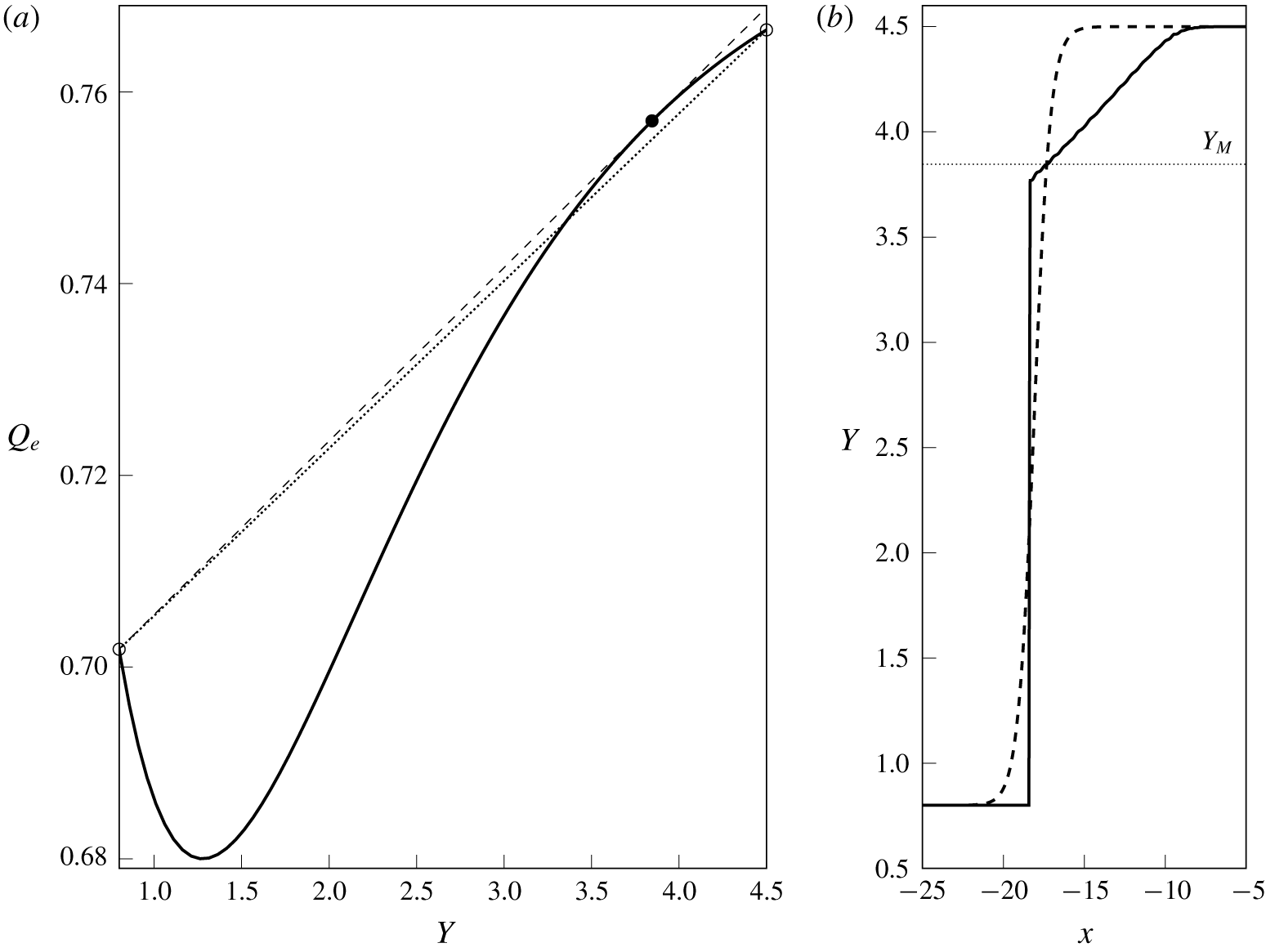
Compound-wave solution to the Riemann problem in the hydraulic limit. The parameters are  $a=1.25$ and
 $\unicode[STIX]{x1D6F1}=-1$, and the initial step goes from
 $Y_{-}=0.8$ to
 $Y_{+}=4.5$. (a) The flux function
 $Q_{e}(Y)$. Open dots show
 $Y_{\pm }$, and the filled dot is
 $Y_{M}$. The dashed line is the chord joining
 $Y_{-}$ to
 $Y_{M}$, and the dotted line is the chord joining
 $Y_{-}$ to
 $Y_{+}$, which intersects the curve and does not satisfy the entropy condition (3.7). (b) The width of the current,
 $Y$, at
 $t=1000$ (solid curve) and the initial condition (dashed curve) translated in
 $x$ for ease of comparison.

Figure 2 shows a numerical simulation of the hydraulic equation (2.12) with  $a=1.25$,
 $\unicode[STIX]{x1D6F1}=-1$ and an initial step chosen so that the entropy condition (3.7) is not satisfied. Starting from a smoothed step, the equation is integrated from
 $t=0$ using the Lax–Wendroff method with Neumann boundary conditions at either end of the computational domain. The solution
 $Y$ is plotted at
 $t=1000$ as the solid curve in figure 2(b). The dashed curve shows the initial step, translated in
 $x$ by
 $1000V_{S}$ for ease of comparison. The shock–rarefaction structure is clear, with the front steepening for
 $Y<Y_{M}$ and relaxing to a rarefaction for
 $Y>Y_{M}$, where
 $Y_{M}=3.85$ is given by the horizontal dotted line. The geometric viewpoint is illustrated in figure 2(a), which shows the flux function
 $Q_{e}(Y)$. The dotted line represents a shock propagating at
 $V_{S}(Y_{+},Y_{-})$, and intersects the curve
 $Q_{e}(Y)$ at
 $Y\approx 3.5$. This shock would therefore fail to satisfy the entropy condition (3.7). Instead the solution develops a shock that joins
 $Y_{-}$ with the intermediate value
 $Y_{M}$, chosen so that the shock speed
 $V_{S}(Y_{M},Y_{-})$ (dashed line in figure 2a) is tangential to
 $Q_{e}$ at
 $Y_{M}$. Thus,
 $Y_{M}$ is the maximum offshore distance of a front that can connect to
 $Y_{-}=0.8$ via a shock.
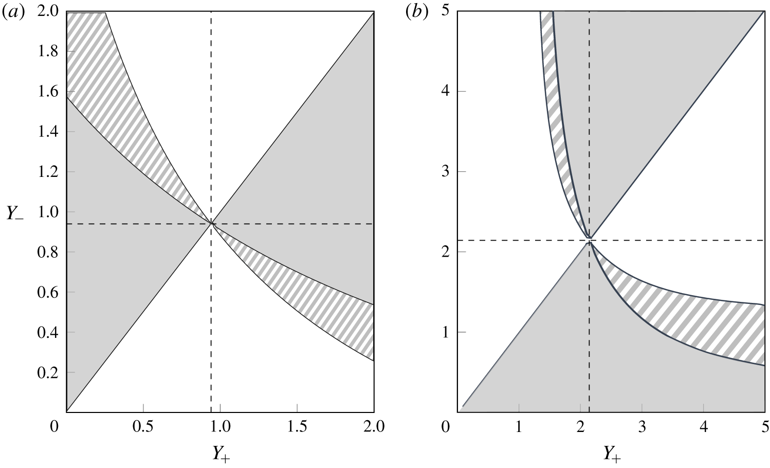
Diagram showing the resolution of the Riemann problem for (a)  $a=2$,
 $\unicode[STIX]{x1D6F1}=1$ and (b)
 $a=1.25$,
 $\unicode[STIX]{x1D6F1}=-1$. In both cases, the dashed lines mark
 $Y_{2}$. Shaded regions show where the initial step is resolved by a shock, white regions correspond to a rarefaction and striped regions correspond to a shock–rarefaction.

Figure 3 shows the classification diagram for the resolution of an initial step in terms of the parameters  $Y_{+}$ and
 $Y_{-}$. Shaded regions of the diagram correspond to initial steps that are resolved by a shock, white regions to steps that are resolved by a rarefaction and striped regions to a shock–rarefaction. Dashed lines show
 $Y_{2}$, the inflection point for
 $Q_{e}$, which divides the classification diagram into four quadrants. Note that the quadrant with
 $Y_{\pm }<Y_{2}$ displays the opposite behaviour to the quadrant with
 $Y_{\pm }>Y_{2}$. The qualitative structure of the classification diagram is the same for any
 $a>1$, although we note that as
 $a\rightarrow 1^{+}$,
 $Y_{2}\rightarrow \infty$ if
 $\unicode[STIX]{x1D6F1}=-1$, but
 $Y_{2}\rightarrow 0$ if
 $\unicode[STIX]{x1D6F1}=1$. If
 $a<1$ the flow is dominated by the Kelvin wave, which is stronger at the coast and so shocks occur when
 $Y_{+}>Y_{-}$. Figure 3 also shows that a shock–rarefaction requires
 $|Y_{+}-Y_{-}|$ to be finite. Indeed if one takes the weakly nonlinear limit of (2.18), with
 $Y=Y_{\infty }+\unicode[STIX]{x1D6E5}$ and
 $|\unicode[STIX]{x1D6E5}|\ll 1$, the resulting equation is the KdV equation unless
 $Y_{\infty }=Y_{2}$, in which case (at next order in
 $\unicode[STIX]{x1D6E5}$) one obtains the modified KdV. Thus compound-wave structures are necessarily a finite-amplitude effect.
Although we have focused on the Riemann problem, the classification diagrams in figure 3 can be used to interpret a wide range of initial conditions  $Y(x,0)$. By considering the sign of
 $\unicode[STIX]{x2202}Y/\unicode[STIX]{x2202}x$, one may place the initial condition just above or below the line
 $Y_{+}=Y_{-}$ and then, by considering the value of
 $Y$, identify which regions of the front will steepen into a shock, and which regions will lengthen into a rarefaction. Any front that crosses
 $Y=Y_{2}$ will form a compound-wave structure. If the flow remains smooth and
 $Q_{e}$ is convex, then adding higher-order terms to the hydraulic equation (2.12) makes little difference, and so figure 3 is also useful for understanding the behaviour of some fronts in the full QG system (2.1). However, in the case of a front that steepens, the gradient
 $\unicode[STIX]{x2202}Y/\unicode[STIX]{x2202}x$ increases and so higher-order dispersive terms become important.
4 The dispersive equation
Here, we consider the dispersive equation (2.18). We first discuss travelling-wave solutions, including the special cases of solitons, kinks and intrusions. These serve as a preliminary to applying El’s technique of ‘dispersive shock-fitting’ (El Reference El2005), which allows the Riemann problem to be classified.
4.1 Travelling-wave solutions to the dispersive equation
When higher-order dispersive terms are added to the hydraulic equation (2.12), shocks no longer form. Instead, wave-steepening leads to DSWs (also called undular bores in the context of water waves) which are a canonical and important structure in nonlinear dispersive wave dynamics (Hoefer & Ablowitz Reference Hoefer and Ablowitz2009). For the purposes of this work we need only note that a DSW is an expanding, slowly modulated waveform, with a linear wavetrain at one end and a solitary wave at the other. Thus to understand shock resolution in the dispersive equation it is necessary to understand the behaviour of both linear waves and solitary waves, which motivates the following, more general, discussion of travelling-wave solutions to (2.18).
First, we write (2.18) in potential form:
 $$\begin{eqnarray}\displaystyle (Y^{\prime })^{2} & = & \displaystyle \frac{2}{a^{2}}\frac{a^{3}\text{e}^{-2Y/a}-4a(\unicode[STIX]{x1D6F1}+a^{2})\text{e}^{-Y/a}+2\unicode[STIX]{x1D6F1}sY^{2}+\unicode[STIX]{x1D6FC}Y+E}{a-(a+2Y)\text{e}^{-2Y/a}}\nonumber\\ \displaystyle & = & \displaystyle \frac{2}{a^{2}}\frac{{\mathcal{V}}(Y;s,\unicode[STIX]{x1D6FC},E)}{{\mathcal{G}}(Y)}.\end{eqnarray}$$
Here, primes ( $^{\prime }$) denote differentiation with respect to the moving coordinate
 $\unicode[STIX]{x1D709}=x-st$,
 $s$ is the speed of the travelling wave and
 $\unicode[STIX]{x1D6FC}$ and
 $E$ are constants of integration (with
 $E$ the ‘energy’ of the orbit). Note that
 ${\mathcal{G}}\geqslant 0$, so that travelling-wave solutions exist whenever
 ${\mathcal{V}}\geqslant 0$ and we may often ignore
 ${\mathcal{G}}$ in our analysis.
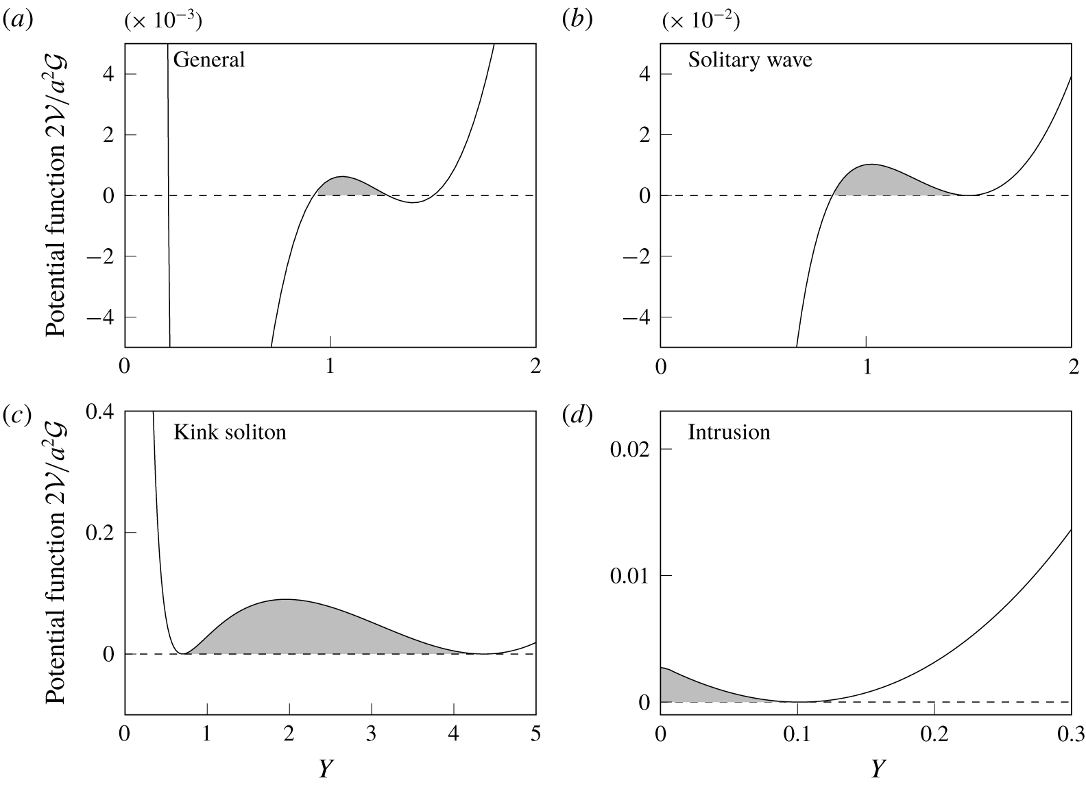
Configurations of the potential function (4.1). (a) The general case, (b) solitary wave case with a local minimum, (c) kink with two double roots and (d) intrusion. In each case, travelling waves exist in the shaded region.

Figure 4 shows four representative examples of (4.1). Figure 4(a) shows the general case, where the numerator  ${\mathcal{V}}$ has four roots. Double roots of
 ${\mathcal{V}}$ at
 $Y=Y_{\infty }$ correspond to linear or solitary waves propagating on the background
 $Y_{\infty }$ depending on whether they are maxima or minima of
 ${\mathcal{V}}$, respectively. Figure 4(b) shows a solitary wave of depression propagating on the background
 $Y_{\infty }=1.5$. There are two special configurations of
 ${\mathcal{V}}$: if
 ${\mathcal{V}}$ has two double roots then the travelling wave is a so-called kink soliton, as in figure 4(c), while if
 ${\mathcal{V}}(0)\geqslant 0$ and there exists a double root in
 $Y>0$, as in figure 4(d), then the solution is a model for a coastal intrusion (i.e. a constant-width current with a ‘nose’). These special cases are discussed in § 4.1.3.
4.1.1 Linear waves
Consider a small disturbance proportional to  $\exp [\text{i}(kx-\unicode[STIX]{x1D714}t)]$, propagating on a background
 $Y_{\infty }$. By making this ansatz in (2.18) we obtain the dispersion relation
 $$\begin{eqnarray}\unicode[STIX]{x1D714}=C(Y_{\infty })k-\frac{a^{2}}{4}\unicode[STIX]{x1D6F1}{\mathcal{G}}(Y_{\infty })k^{3},\end{eqnarray}$$
and the phase speed
 $$\begin{eqnarray}s_{L}=\frac{\unicode[STIX]{x1D714}}{k}=C(Y_{\infty })-\frac{a^{2}}{4}\unicode[STIX]{x1D6F1}{\mathcal{G}}(Y_{\infty })k^{2},\end{eqnarray}$$
which corresponds to advection by the background flow and a dispersive term with sign  $-\unicode[STIX]{x1D6F1}$. In § 6, we compare (4.2) with other dispersion relations that have previously been derived for long frontal waves.
4.1.2 Solitary waves
The potential equation (4.1) admits solitary-wave solutions for certain values of the parameters  $s$,
 $\unicode[STIX]{x1D6FC}$ and
 $E$. It is convenient to ignore
 ${\mathcal{G}}$, and seek the range of speeds
 $s$ for which solitary waves exist.
Thus, consider a solitary wave propagating on the background  $Y_{\infty }$. Then
 ${\mathcal{V}}(Y_{\infty })=0$ and
 ${\mathcal{V}}^{\prime }(Y_{\infty })=0$, which sets
 $E$ and
 $\unicode[STIX]{x1D6FC}$ as functions of
 $Y_{\infty }$ and
 $s$ in (4.1). Further,
 ${\mathcal{V}}(Y_{\infty })$ must be a local minimum. This requires
 $$\begin{eqnarray}\displaystyle \left.\begin{array}{@{}c@{}}s>C(Y_{\infty })\quad \text{when }\unicode[STIX]{x1D6F1}=1,\\ s<C(Y_{\infty })\quad \text{when }\unicode[STIX]{x1D6F1}=-1,\end{array}\right\} & & \displaystyle\end{eqnarray}$$
which, as expected, sets the minimum (maximum) speed for solitary waves on a current with positive (negative) PVa to be the long-wave speed  $C(Y_{\infty })$. A solitary wave of depression occurs if
 ${\mathcal{V}}$ has a root, say
 $Y_{S}$, in
 $[0,Y_{\infty })$. Thus a depression wave occurs if, in addition to (4.3),
 ${\mathcal{V}}(0)\leqslant 0$ or
 $$\begin{eqnarray}\displaystyle \left.\begin{array}{@{}c@{}}s<s_{0}\quad \text{when }\unicode[STIX]{x1D6F1}=1,\\ s>s_{0}\quad \text{when }\unicode[STIX]{x1D6F1}=-1,\end{array}\right\} & & \displaystyle\end{eqnarray}$$
where we have introduced the critical speed
 $$\begin{eqnarray}s_{0}=Y_{\infty }^{-2}\left[2a+\frac{3a^{3}\unicode[STIX]{x1D6F1}}{2}-2(1+a^{2}\unicode[STIX]{x1D6F1})(a+Y_{\infty })\text{e}^{-Y_{\infty }/a}+\frac{a^{2}\unicode[STIX]{x1D6F1}}{2}(a+2Y_{\infty })\text{e}^{-2Y_{\infty }/a}\right].\end{eqnarray}$$
The amplitude of the wave is  $Y_{\infty }-Y_{S}$. A solitary wave that travels close to speed
 $s_{0}$ extends from
 $Y_{\infty }$ to
 $Y=0^{+}$. For
 $s$ beyond
 $s_{0}$,
 ${\mathcal{V}}(0)>0$ and, provided there is no other root in
 $[0,Y_{\infty })$, the corresponding travelling-wave solution extends to the coast and can be used to model a coastal intrusion, as in figure 4(d).
Next, note that a solitary wave of elevation occurs if  ${\mathcal{V}}$ has a root
 $Y_{S}$ in
 $(Y_{\infty },\infty )$. As
 $Y\rightarrow \infty$,
 ${\mathcal{V}}\sim s\unicode[STIX]{x1D6F1}Y^{2}$, so that a sufficient condition for an elevation wave is
 $\unicode[STIX]{x1D6F1}s<0$. However, elevation waves may also exist for
 $\unicode[STIX]{x1D6F1}s>0$, provided
 $Y_{S}$ exists. The limiting case for the existence of the additional root occurs when
 ${\mathcal{V}}^{\prime }(Y_{S})=0$, so that
 ${\mathcal{V}}$ has two double roots and the corresponding travelling-wave solution is a kink soliton. Given
 $a$,
 $\unicode[STIX]{x1D6F1}$ and
 $Y_{\infty }$, we seek a pair
 $(s_{K},Y_{K})$ such that
 $V(Y_{K})=V^{\prime }(Y_{K})=0$, with
 $Y_{K}>Y_{\infty }$. The kink soliton connects the equilibria
 $Y_{\infty }$ and
 $Y_{K}$, and travels at speed
 $s_{K}$. Since the kink is the limiting case of an elevation wave,
 $Y_{K}$ is an upper bound on the soliton amplitude and
 $s_{K}$ is the maximum (minimum) speed for a solitary wave of elevation on a current with positive (negative) PVa.
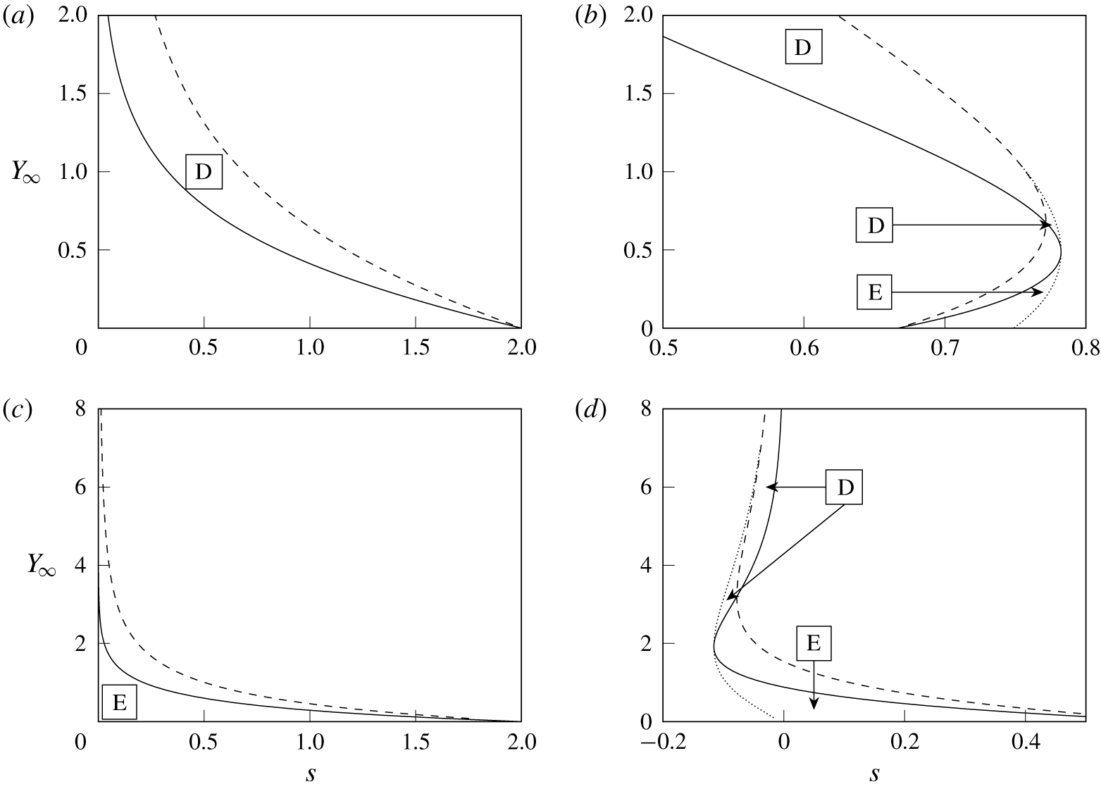
Possible solitary wave speeds  $s$ as a function of the background
 $Y_{\infty }$. The solid, dashed and dotted curves are
 $C$,
 $s_{0}$ and
 $s_{K}$, respectively. Waves of elevation exist in regions marked E, and waves of depression exist in regions marked D. The parameters
 $a$ and
 $\unicode[STIX]{x1D6F1}$ are chosen so that each plot shows a different regime: (a)
 $\unicode[STIX]{x1D6F1}=1$,
 $a=0.5$; (b)
 $\unicode[STIX]{x1D6F1}=1$,
 $a=1.5$; (c)
 $\unicode[STIX]{x1D6F1}=-1$,
 $a=0.5$; (d)
 $\unicode[STIX]{x1D6F1}=-1$,
 $a=1.5$.

By combining all of the above, we may determine the range of allowed solitary wave speeds  $s$ as a function of
 $\unicode[STIX]{x1D6F1}$,
 $a$ and the background state
 $Y_{\infty }$. We find that there are four regimes, depending on the value of
 $\unicode[STIX]{x1D6F1}$ and
 $a$. An example of each regime is shown in figure 5, where the limiting values
 $C$,
 $s_{0}$ and
 $s_{K}$ are plotted as functions of
 $Y_{\infty }$ as the solid, dashed and dotted curves, respectively. Depression waves exist in regions of the
 $(s,Y_{\infty })$-plane marked D, and elevation waves exist in regions marked E. The solitary waves are of vanishing amplitude close to the solid curve
 $C(Y_{\infty })$, and reach maximum amplitude at the dashed or dotted curve (or at
 $s=0$ in the case of figure 5(c), where the solitary wave has infinite amplitude). For small
 $a$, the curves
 $s_{0}$ and
 $C$ do not intersect and only one type of solitary wave is possible (figure 5a,c). For
 $a$ sufficiently large, the two curves intersect and so both elevation and depression waves (as well as kinks) exist, with depression waves existing for
 $Y_{\infty }>Y_{2}$ (figures 5b or 5d). The intersection between
 $s_{0}$ and
 $C$ occurs for the first time when
 $a=1$ if
 $\unicode[STIX]{x1D6F1}=1$, and when
 $a=2/\surd 3$ if
 $\unicode[STIX]{x1D6F1}=-1$. (The critical value of
 $a$ when
 $\unicode[STIX]{x1D6F1}=-1$ can be determined by considering the sign of
 $s_{0}-C$ for large
 $Y_{\infty }$.)
4.1.3 Special cases
We now discuss the two special cases mentioned above: the kink soliton and the coastal intrusion. Kink solitons require that  ${\mathcal{V}}$ has two double roots, say
 $Y_{\infty }$ and
 $Y_{K}$, which correspond to the two far-field states connected by the travelling wave. It turns out that this configuration is only possible if
 $a$ is sufficiently large (
 $a>1$ when
 $\unicode[STIX]{x1D6F1}=1$, and
 $a>2/\surd 3$ when
 $\unicode[STIX]{x1D6F1}=-1$). The propagation speed
 $s_{K}(Y_{\infty })$ is plotted as a dotted curve in figure 5(b,d). We find that
 $s_{K}(Y_{\infty })$ has a turning point at
 $Y_{2}$, the turning point for the long-wave speed
 $C(Y)$. Each
 $s_{K}$ is associated with two background states, one on either side of
 $Y_{2}$, and the kink soliton connects these two states. Thus the kink is a result of the non-convexity of the flux function
 $Q_{e}$, as in the modified KdV equation. Kink solitons are of particular interest because they are travelling-wave solutions that connect two different far-field states, and thus are analogous to shock-wave solutions to the hydraulic equation. However,
 $s_{K}$ does not lie between
 $C(Y_{\infty })$ and
 $C(Y_{K})$, so the propagation speed does not satisfy the entropy condition (3.7). The kink soliton is therefore sometimes referred to as a non-classical or under-compressive shock wave (El, Hoefer & Shearer Reference El, Hoefer and Shearer2017). Kinks will later be shown to play an important role in the Riemann problem when the initial step crosses
 $Y_{2}$.
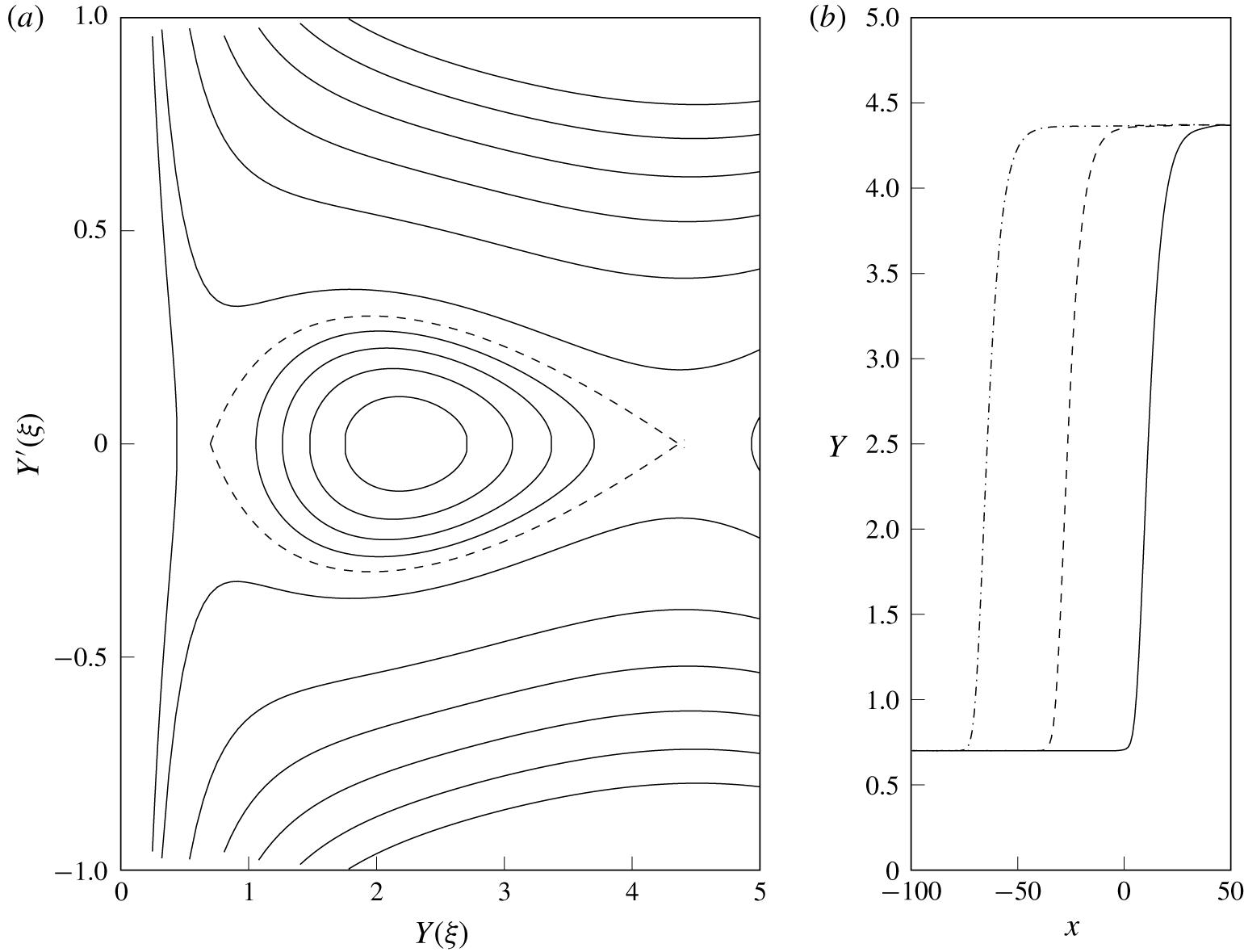
Kink soliton connecting  $Y_{\infty }=0.7$ with
 $Y_{K}=4.41$, with
 $a=1.5$,
 $\unicode[STIX]{x1D6F1}=-1$. (a) The phase portrait with
 $s=s_{K}=-0.076$. The dashed curve is the kink orbit, with curves inside corresponding to periodic waves. (b) Propagation of the kink soliton in (2.18). The solid, dashed and dash-dotted curves show the solution at
 $t=0$, 500 and 1000, respectively.

Figure 6 shows the kink soliton solution propagating on the background  $Y_{\infty }=0.7$ with
 $\unicode[STIX]{x1D6F1}=-1$ and
 $a=1.5$, which are the values used for the potential function in figure 4(c). The phase portrait for travelling-wave solutions propagating at speed
 $s_{K}=-0.076$ is shown in figure 6(a). There are saddle points at
 $Y_{\infty }$ and
 $Y_{K}=4.37$, and a centre at
 $Y\approx 2$. The kink soliton is represented by the heteroclinic orbit connecting the two saddle points, which is shown dashed. Closed orbits inside the dashed curve correspond to lower-energy periodic waves. Figure 6(b) shows a numerical solution to (2.18) when the kink soliton is used as an initial condition (solid curve). The dashed and dash-dotted curves show the solution at
 $t=500$ and
 $t=1000$, respectively, and confirm that the kink propagates at constant speed
 $s_{K}$.
Here and elsewhere, numerical results are obtained using a pseudo-spectral method, where the equation is Fourier-transformed in  $x$ and then advanced in time using an adaptive fourth-order Runge–Kutta scheme. The domain is truncated at some large value of
 $x$, and a corresponding step down from
 $Y_{K}$ to
 $Y_{\infty }$ is introduced to enforce the periodicity required by the spectral method. The domain is taken large enough so that the two steps do not interfere with each other. The equation is solved using the long-wave coordinates
 $X$ and
 $T$, but results are plotted in the original coordinates
 $x$ and
 $t$. In all results shown, the long-wave parameter
 $\unicode[STIX]{x1D716}=0.1$.
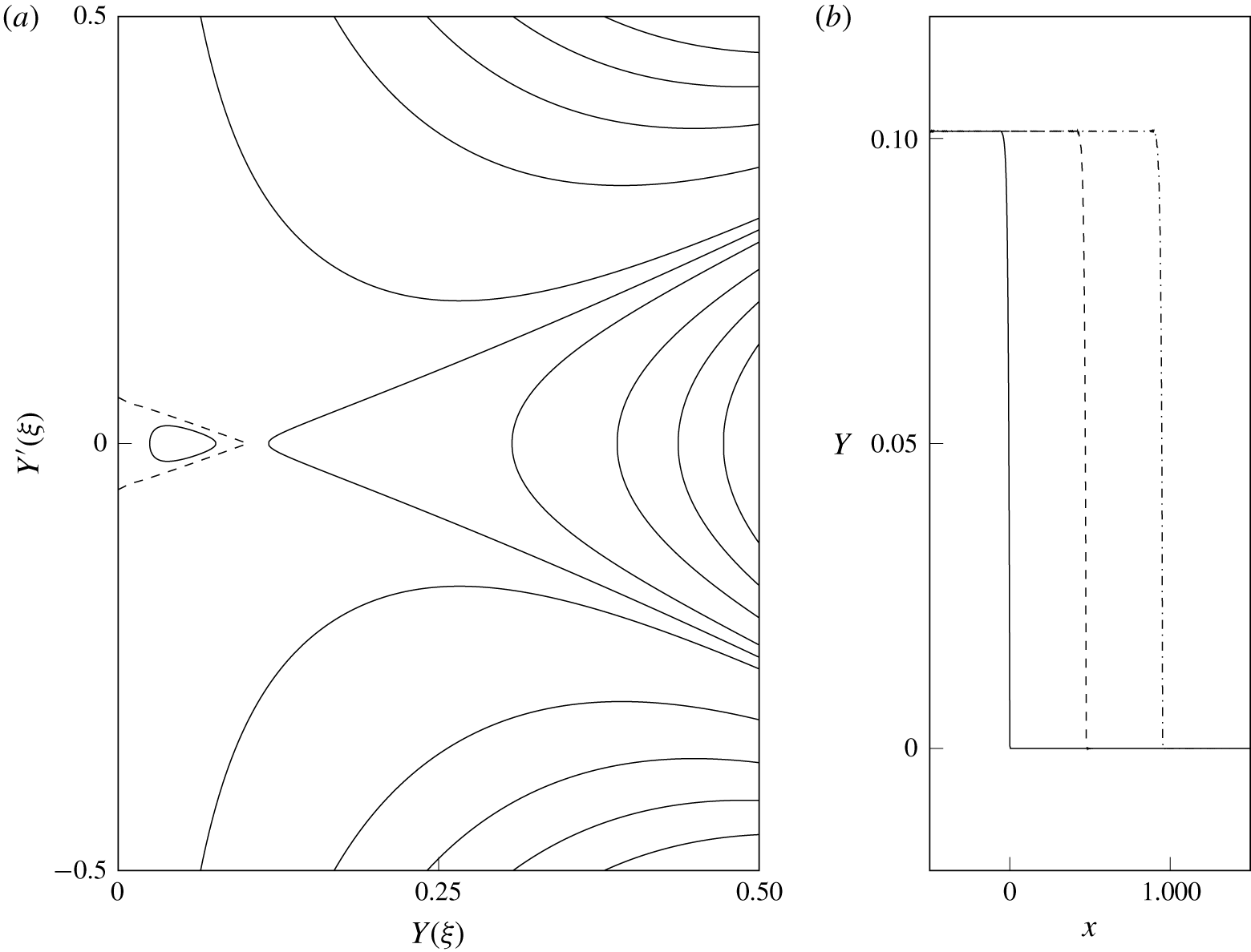
Coastal intrusion of permanent form, with  $a=1.05$ and
 $\unicode[STIX]{x1D6F1}=1$. (a) The phase portrait with
 $s=s_{K}=0.95$. The dashed curve is the intrusion orbit, with the curve inside corresponding to a periodic travelling wave. (b) Propagation of the intrusion, with the solution shown at
 $t=0$, 500 and 1000 (solid, dashed and dash-dotted curves, respectively).

If the condition (4.4) is not satisfied, the corresponding travelling-wave solution reaches  $Y=0$ and may be joined to a constant-width current to give a model for a coastal intrusion of permanent form. Letting
 $Y\rightarrow 0$ in (4.1) we see that the nose of the intrusion meets the coast at right angles unless
 ${\mathcal{V}}$ has a double root at zero; that is, unless the intrusion is a kink soliton with background
 $Y_{\infty }=0$. In this case, the front meets the coast with
 $$\begin{eqnarray}(Y^{\prime })^{2}=\frac{2\unicode[STIX]{x1D6F1}(as_{K}-1)}{a^{2}}.\end{eqnarray}$$
Such an intrusion is shown in figure 7, for  $\unicode[STIX]{x1D6F1}=1$ and
 $a=1.05$, which are the values used for figure 4(d). The phase portrait in figure 7(a) has a saddle point at
 $Y_{K}=0.101$, but since
 ${\mathcal{G}}(0)$ is infinite, the double root in
 ${\mathcal{V}}$ does not lead to a saddle point at
 $Y=0$. Figure 7(b) shows the evolution of the intrusion at
 $t=0$, 500 and 1000 (solid, dashed and dash-dotted curves, respectively). We performed other numerical experiments (not shown) using a solitary wave intrusion that meets the coast at right angles. The infinite gradient at
 $Y=0$ led to a build-up of spurious short waves, which quickly grew and disturbed the intrusion.
The intrusion of a PV front is discussed at length for a dam-break scenario in Stern & Helfrich (Reference Stern and Helfrich2002). The authors seek similarity solutions to the long-wave equations and find that the nose is always a rarefying intrusion, a result that is supported by numerical and laboratory experiments. Johnson et al. (Reference Johnson, Southwick and McDonald2017) also find that PV intrusions driven by a uniform source either rarefy or form shocks. Thus although intrusions of permanent form are valid solutions to the equations, at least in the QG limit, it is not clear what initial conditions would give rise to one.
4.2 The Riemann problem for the dispersive equation
El’s technique of dispersive shock-fitting is based on the approach of Gurevich & Pitaevskii (Reference Gurevich and Pitaevskii1973) to solving the Riemann problem for the KdV equation, but generalised to deal with a wider class of (non-integrable) equations. The key idea in the approach of Gurevich & Pitaevskii (Reference Gurevich and Pitaevskii1973) is that the Whitham equations (i.e. the period-averaged equations) governing the modulation of the DSW can be matched naturally to the hydraulic equation in the far field. Provided that the equation under consideration satisfies certain conditions, El’s technique allows one to obtain the propagation speeds of the DSW edges, the wavenumber at the linear edge and the conjugate wavenumber (i.e. the inverse half-width) and amplitude at the soliton edge. El (Reference El2005) gives a full explanation of the theory and the derivation of the necessary conditions, and Kamchatnov (Reference Kamchatnov2019) and Maiden et al. (Reference Maiden, Franco, Webb, El and Hoefer2020) adapt El’s technique to other initial conditions.
4.2.1 Applicability of El’s technique
For El’s technique to apply, the dispersive equation (2.18) must satisfy the following conditions:
(i) It admits a dispersionless (hydraulic) limit obtained by introducing the slow variables
$X=\unicode[STIX]{x1D716}x$ and $T=\unicode[STIX]{x1D716}t$. By construction, this is true.(ii) The linear dispersion relation
$\unicode[STIX]{x1D714}(k)$ is real-valued. This was shown in (4.2a).(iii) It possesses at least two conservation laws. This is required so that the Whitham system of averaged conservation laws can be formulated in principle, although El’s technique is designed to avoid this. These may be taken as the kinematic boundary condition (2.7b) and (2.19).
(iv) It supports periodic travelling-wave solutions, parameterised by three independent variables. These can be taken to be the constants of integration
$s$, $\unicode[STIX]{x1D6FC}$ and $E$ in the potential (4.1). The potential function must have at least three real zeros (in general (4.1) has four, as in figure 4a), and must exhibit quadratic behaviour in the linear- and solitary-wave limits. This condition allows the Whitham equations to be matched with the hydraulic equation at the edges of the DSW. The necessary quadratic behaviour is shown below.(v) The Whitham system corresponding to the two averaged conservation laws plus the wavenumber conservation law
$k_{t}+\unicode[STIX]{x1D714}_{x}=0$ is hyperbolic. Hyperbolicity cannot be checked without directly solving the Whitham system so this condition should be verified by, for example, comparison of theoretical results with numerical simulations. However, non-convexity of the flux function $Q_{e}$ implies that (2.18) is not genuinely nonlinear (the characteristic velocity $C$ is not monotonic), and in many cases this leads to non-strict hyperbolicity (El et al. Reference El, Hoefer and Shearer2017). The compound-wave structures discussed in § 3.1 carry over to the Whitham equations, and lead to richer behaviour than in the simple-wave case, where the solution is a DSW. El’s technique should therefore only be applied to initial steps that do not straddle $Y_{2}$, so that the flux function is convex. The effects of non-convexity are discussed in § 5.2.


It remains to show that the potential function (4.1) displays quadratic behaviour in the linear- and solitary-wave limits. Essentially, we would like to show that in these limits
 $$\begin{eqnarray}\frac{2}{a^{2}}\frac{{\mathcal{V}}(Y;s,\unicode[STIX]{x1D6FC},E)}{{\mathcal{G}}(Y)}\sim (Y-Y_{\infty })^{2}\unicode[STIX]{x1D6F7}(Y),\end{eqnarray}$$
where  $Y_{\infty }$ is the solitary- or linear-wave background and
 $\unicode[STIX]{x1D6F7}(Y)=O(1)$ for
 $|Y-Y_{\infty }|\ll 1$. In both limits,
 $\unicode[STIX]{x1D6FC}$ and
 $E$ may be written as functions of
 $s$ and
 $Y_{\infty }$, so may be taken as fixed. Unless
 $Y_{\infty }\ll 1$ and the front is close to the coast,
 ${\mathcal{G}}=O(1)$ and it is sufficient to check the behaviour of
 ${\mathcal{V}}(Y;s,Y_{\infty })$. Since
 $Y_{\infty }$ is a double root of
 ${\mathcal{V}}$, the potential function displays the quadratic behaviour (4.6) provided
 ${\mathcal{V}}^{\prime \prime }(Y_{\infty })$ is non-zero, i.e. by (4.3)
 $s$ is sufficiently far from the long-wave speed
 $C(Y_{\infty })$.
4.2.2 Dispersive shock-fitting
With these caveats about non-convexity and distance from the coast in mind, El’s technique proceeds as follows. The wavenumber and conjugate wavenumber at the linear- and solitary-wave edges of the DSW are found by solving the ordinary differential equations
 $$\begin{eqnarray}\displaystyle \left.\begin{array}{@{}c@{}}{\displaystyle \frac{\text{d}k}{\text{d}Y}}={\displaystyle \frac{\unicode[STIX]{x2202}\unicode[STIX]{x1D714}/\unicode[STIX]{x2202}Y}{C(Y)-\unicode[STIX]{x2202}\unicode[STIX]{x1D714}/\unicode[STIX]{x2202}k}},\\ {\displaystyle \frac{\text{d}\tilde{k}}{\text{d}Y}}={\displaystyle \frac{\unicode[STIX]{x2202}\tilde{\unicode[STIX]{x1D714}}/\unicode[STIX]{x2202}Y}{C(Y)-\unicode[STIX]{x2202}\tilde{\unicode[STIX]{x1D714}}/\unicode[STIX]{x2202}\tilde{k}}}.\end{array}\right\} & & \displaystyle\end{eqnarray}$$
Here,  $\tilde{k}$ is the conjugate wavenumber and
 $\tilde{\unicode[STIX]{x1D714}}=-\text{i}\unicode[STIX]{x1D714}(Y,\text{i}\tilde{k})$ is the conjugate dispersion relation for solitary waves. The fact that the solitary-wave propagation speed can be described by linear-wave dynamics can be seen by considering the exponential tail. If the tail is proportional to
 $\exp (\tilde{k}x-\tilde{\unicode[STIX]{x1D714}}t)$ then it obeys a linear dispersion relation
 $\tilde{\unicode[STIX]{x1D714}}$ as defined above, with propagation speed
 $s=\tilde{\unicode[STIX]{x1D714}}/\tilde{k}$ (Kamchatnov Reference Kamchatnov2019). The ordinary differential equations (4.7) are derived in El (Reference El2005) using the ansatz
 $k=k(Y)$ in the wavenumber conservation law, combined with the hydraulic equation (2.12) which is assumed to apply at the edge of the DSW. The general solutions to (4.7) are
 $$\begin{eqnarray}\displaystyle \left.\begin{array}{@{}c@{}}k^{2}(Y)={\displaystyle \frac{8\unicode[STIX]{x1D6F1}}{3a^{2}{\mathcal{G}}(Y)^{2/3}}}\displaystyle \int ^{Y}{\displaystyle \frac{C^{\prime }(\unicode[STIX]{x1D709})}{{\mathcal{G}}(\unicode[STIX]{x1D709})^{1/3}}}\,\text{d}\unicode[STIX]{x1D709},\\ \tilde{k}^{2}(Y)={\displaystyle \frac{-8\unicode[STIX]{x1D6F1}}{3a^{2}{\mathcal{G}}(Y)^{2/3}}}\displaystyle \int ^{Y}{\displaystyle \frac{C^{\prime }(\unicode[STIX]{x1D709})}{{\mathcal{G}}(\unicode[STIX]{x1D709})^{1/3}}}\,\text{d}\unicode[STIX]{x1D709}.\end{array}\right\} & & \displaystyle\end{eqnarray}$$
To connect (4.8) with the far-field solution, we apply the boundary conditions  $k=0$ at the soliton edge of the DSW, and
 $\tilde{k}=0$ at the linear-wave end. Then we may obtain
 $k_{\pm }$ and
 $\tilde{k}_{\mp }$, the wavenumber and conjugate wavenumber at the leading/trailing edge of the DSW, by evaluating (4.8) at
 $Y_{\pm }$. Bearing in mind the form of the dispersion relation (4.2a) and the restriction on soliton speed (4.3), it is clear that DSWs have solitary waves on the right when
 $\unicode[STIX]{x1D6F1}=1$ and on the left when
 $\unicode[STIX]{x1D6F1}=-1$. Thus if
 $\unicode[STIX]{x1D6F1}=1$ we have
 $$\begin{eqnarray}\displaystyle \left.\begin{array}{@{}c@{}}k_{-}^{2}={\displaystyle \frac{8}{3a^{2}{\mathcal{G}}(Y_{-})^{2/3}}}\displaystyle \int _{Y_{+}}^{Y_{-}}{\displaystyle \frac{C^{\prime }(Y)}{{\mathcal{G}}(Y)^{1/3}}}\,\text{d}Y,\\ \tilde{k}_{+}^{2}={\displaystyle \frac{8}{3a^{2}{\mathcal{G}}(Y_{+})^{2/3}}}\displaystyle \int _{Y_{+}}^{Y_{-}}{\displaystyle \frac{C^{\prime }(Y)}{{\mathcal{G}}(Y)^{1/3}}}\,\text{d}Y\end{array}\right\} & & \displaystyle\end{eqnarray}$$
for the trailing linear and leading solitary wavenumbers, while if  $\unicode[STIX]{x1D6F1}=-1$ we have
 $$\begin{eqnarray}\displaystyle \left.\begin{array}{@{}c@{}}k_{+}^{2}={\displaystyle \frac{8}{3a^{2}{\mathcal{G}}(Y_{+})^{2/3}}}\displaystyle \int _{Y_{+}}^{Y_{-}}{\displaystyle \frac{C^{\prime }(Y)}{{\mathcal{G}}(Y)^{1/3}}}\,\text{d}Y,\\ \tilde{k}_{-}^{2}={\displaystyle \frac{8}{3a^{2}{\mathcal{G}}(Y_{-})^{2/3}}}\displaystyle \int _{Y_{+}}^{Y_{-}}{\displaystyle \frac{C^{\prime }(Y)}{{\mathcal{G}}(Y)^{1/3}}}\,\text{d}Y\end{array}\right\} & & \displaystyle\end{eqnarray}$$
for the trailing solitary and leading linear wavenumbers. Note that since El’s method is restricted to initial steps that do not cross  $Y_{2}$,
 $C^{\prime }(Y)$ is single-signed and (4.9) is real provided
 $Y_{\pm }$ are taken from the shaded region in figure 3, i.e. provided that the corresponding step in the hydraulic equation leads to a shock rather than a rarefaction.
The propagation speeds of the solitary- and linear-wave ends of the DSW are
 $$\begin{eqnarray}s_{\pm }=\frac{\tilde{\unicode[STIX]{x1D714}}(Y_{\pm },\tilde{k}_{\pm })}{\tilde{k}_{\pm }},\quad s_{\mp }=\frac{\unicode[STIX]{x2202}\unicode[STIX]{x1D714}}{\unicode[STIX]{x2202}k}\bigg|_{Y_{\mp },k_{\mp }},\end{eqnarray}$$
when  $\unicode[STIX]{x1D6F1}=\pm 1$. Finally, the following inequalities must be verified:
 $$\begin{eqnarray}s_{-}<C_{-},\quad s_{+}>C_{+},\quad s_{+}>s_{-}.\end{eqnarray}$$
The first two of these conditions are analogous to the entropy condition (3.7), and ensure that characteristics from the external, hydraulic solution transfer information into the DSW. In fact, they are trivially satisfied by (4.9). The third condition checks that the DSW has positive width. We must also check that the solitary wave speed given by El’s technique is valid according to the discussion of § 4.1.2, where we identify the background  $Y_{\infty }$ with
 $Y_{\pm }$ when
 $\unicode[STIX]{x1D6F1}=\pm 1$.
5 Numerical results
Here, we present numerical solutions to the dispersive long-wave equation (2.18) and the full QG equation (2.1). The former are compared with predictions for propagation speed and solitary-wave amplitude that were derived in § 4.2.2 using El’s technique, while the QG equations are used to test the validity of the long-wave approximation.
5.1 Verification of El’s technique
We begin with numerical simulations of the dispersive equation. All computations are carried out using the pseudo-spectral method described in § 4.1.3.
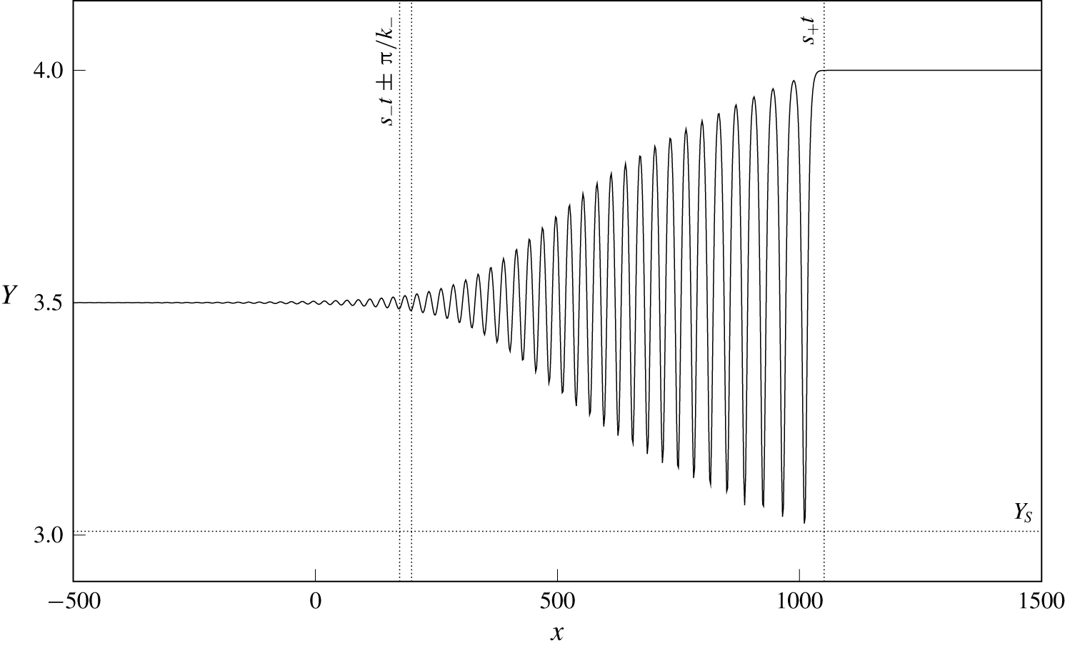
Numerical solution to the Riemann problem for the dispersive equation (2.18). The parameters are  $a=0.9$ and
 $\unicode[STIX]{x1D6F1}=1$ and the smoothed initial step is from
 $Y_{-}=3.5$ to
 $Y_{+}=4$. The solution is shown at
 $t=30\,000$. Dotted lines correspond to theoretical predictions from § 4.2.2.

Figure 8 shows the result for a current with positive PVa and  $a=0.9$. The Riemann problem is initialised with a smoothed step from
 $Y_{-}=3.5$ to
 $Y_{+}=4$, and the solution is shown at
 $t=30\,000$. Since
 $a<1$ and
 $\unicode[STIX]{x1D6F1}=1$, from figure 5 we know that only solitary waves of depression exist. Further, from § 4.2.2 we know that currents with positive PVa are led by a solitary wave. This is clearly visible in figure 8, along with the internal structure of the DSW. Dotted lines show predictions from El’s technique. The horizontal line at
 $Y=Y_{S}$ and the vertical line at
 $x=s_{+}t$ show good agreement between theory and numerics at the solitary-wave edge of the DSW. The two vertical lines on the left-hand side are at
 $x=s_{-}t\pm \unicode[STIX]{x03C0}/k_{-}$ and therefore span one wavelength at the trailing edge of the DSW. The numerical solution has a small-amplitude wave of the correct wavelength at
 $x=s_{-}t$ but, as is typical in simulations of such problems, the amplitude is clearly non-zero for
 $x<s_{-}t$. The amplitude discrepancy is likely due to higher-order (numerical) dispersive effects (Congy et al. Reference Congy, El, Hoefer and Shearer2019). The integration in figure 8 was continued until
 $t=50\,000$. At the point at which the integration was halted, the minimum value of
 $Y$ was still decreasing, but at a rate of
 $O(10^{-6})$ so that the DSW was, for all intents and purposes, fully developed. The minimum value of
 $Y$ and the mean propagation speed of the leading solitary wave agree with the theoretical predictions for
 $Y_{S}$ and
 $s_{+}$ to three decimal places.
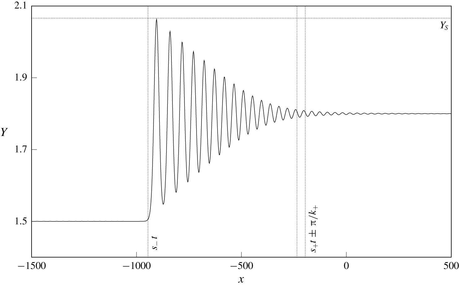
As figure 8, but for a current with negative PVa and  $a=1.25$. The initial step is from
 $Y_{-}=1.5$ to
 $Y_{+}=1.8$ and the solution is shown at
 $t=30\,000$.

Figure 9 shows a current with negative PVa and  $a=2$, with the initial step connecting
 $Y_{-}=1.5$ and
 $Y_{+}=1.8$. As predicted for currents with negative PVa, the DSW has a solitary wave on the left. Only elevation waves exist for the background
 $Y_{\infty }=Y_{-}<Y_{2}$. The solution is shown at
 $t=30\,000$, and the integration was continued until
 $t=50\,000$. Again, the solitary-wave amplitude and propagation speed agree with theoretical predictions to three decimal places while at the linear end of the DSW there is good agreement in wavenumber
 $k_{+}$ and, as above, small waves in
 $x>s_{+}t$.
5.2 Effects of non-convexity
If the initial step crosses the inflection point  $Y_{2}$ the flux function
 $Q_{e}$ is non-convex, so the hydraulic limit is not genuinely nonlinear and El’s technique cannot be directly applied. In this case, numerical results show that the Riemann problem is resolved by a compound-wave structure, as discussed for the modified KdV equation in El et al. (Reference El, Hoefer and Shearer2017) and the Miyata–Camassa–Choi equations in Esler & Pearce (Reference Esler and Pearce2011).
As figure 8, but for an initial step that crosses the inflection point  $Y_{2}$. The parameters are
 $a=2$ and
 $\unicode[STIX]{x1D6F1}=1$, and the solution is shown at
 $t=50\,000$. (a) Initial step down from
 $Y_{-}=1.2$ to
 $Y_{+}=0.6$. (b) Initial step up from
 $Y_{-}=0.6$ to
 $Y_{+}=1.2$. In both cases, the step is resolved by a compound-wave structure involving a kink soliton (see text).

Figure 10 shows two examples of compound-wave structures in a current with  $a=2$ and
 $\unicode[STIX]{x1D6F1}=1$. In both cases, the initial step is resolved by a combination of a kink soliton and a simple wave (DSW or rarefaction), with an expanding constant-width region that connects the two. For currents with positive PVa, the kink is faster than any solitary wave or rarefaction and so must be on the right. Thus in both cases the kink connects
 $Y_{+}$ to the (uniquely determined) intermediate value
 $Y_{K}$. The rightmost vertical line gives the predicted location of the kink,
 $x=s_{K}t$. As in Esler & Pearce (Reference Esler and Pearce2011), it seems that the simple-wave structure can be understood by applying El’s technique to the ‘secondary’ Riemann problem with an initial step from
 $Y_{-}$ to
 $Y_{K}$. In figure 10(a), where
 $Y_{K}>Y_{-}>Y_{2}$, we would expect this secondary step to be resolved by a DSW, led by a solitary wave of depression. This is indeed the case, and El’s technique captures the amplitude and speed at the leading edge of the DSW, as well as the wavenumber at the trailing edge. In figure 10(b),
 $Y_{-}<Y_{K}<Y_{2}$ so that the secondary step is resolved by a rarefaction over the region
 $C(Y_{-})<x/t<C(Y_{K})$.
Note that, in both cases shown in figure 10, the step ‘splits’ into a steadily propagating kink, which crosses the inflection point, and a secondary, simple-wave structure that lies within the convex region of the flux function. Thus the kink can be thought of as removing the non-convexity from the initial step. For the present equation the kink soliton exists provided the background state (here  $Y_{+}$) is less than some critical value (see the termination of the dotted curve
 $s_{K}$ in figure 5b,d). It is not clear how the initial step should be resolved if
 $Y_{+}$ is greater than the critical value. Numerical simulations suggest that the solution passes through
 $Y=0$, which is clearly unphysical. El et al. (Reference El, Hoefer and Shearer2017) introduced a new type of DSW, the so-called contact DSW, to resolve the Riemann problem in the modified KdV equation for steps where the kink does not exist, but the treatment of this case appears to involve solving the Whitham system and so is not pursued here. It is notable that, unlike for the modified KdV equation, the existence of the kink in the present model does not depend on the sign of the dispersion. Finally we note that for the initial step in figure 10(b),
 $C_{+}>C_{-}$. Thus in the hydraulic limit the Riemann problem would be resolved by a simple-wave rarefaction, and so the dispersive terms can dramatically modify even a smooth solution when the flux function is non-convex (see El et al. (Reference El, Hoefer and Shearer2017), comparing § 4 and figure 5.3). The classification diagram for the dispersive Riemann problem is therefore quite different from that for the hydraulic problem shown in figure 3.
5.3 Classification of the dispersive Riemann problem
Diagram showing the resolution of the dispersive Riemann problem for (a)  $a=2$,
 $\unicode[STIX]{x1D6F1}=1$ and (b)
 $a=1.5$,
 $\unicode[STIX]{x1D6F1}=-1$. Labels correspond to kinks, rarefactions and DSWs, with the superscript
 $\text{DSW}^{\pm }$ signifying elevation or depression solitary waves. The hatched regions of the diagram cannot be classified using El’s technique.

Figure 11 classifies the resolution of the initial step  $Y_{\pm }$ for the particular choice of parameters
 $a=2$,
 $\unicode[STIX]{x1D6F1}=1$ (figure 11a) and
 $a=1.5$,
 $\unicode[STIX]{x1D6F1}=-1$ (figure 11b). Hatched regions of the diagram show where the initial step cannot be classified using El’s technique. We have labelled the diagram following the notation of El et al. (Reference El, Hoefer and Shearer2017), whereby K, R and
 $\text{DSW}^{\pm }$ correspond to kinks, rarefactions and DSWs of elevation/depression, respectively. Compound-wave structures are denoted by a vertical bar (
 $|$) and should be read from left to right so that, for example,
 $\text{K}|\text{DSW}^{+}$ means that the initial step is resolved by a kink from
 $Y_{-}$ to
 $Y_{K}$, and a DSW with a solitary wave of elevation connecting
 $Y_{K}$ to
 $Y_{+}$. As discussed in § 4.2.2, DSWs that form on currents with positive PVa have solitary waves on the right, while those on currents with negative PVa have solitary waves on the left.
As in the hydraulic classification diagram in figure 3, for vortically dominated currents with  $a>1$ the
 $Y_{\pm }$ parameter space is split into four quadrants by the inflection point
 $Y_{2}$. Kelvin-wave-dominated flows with
 $a<1$ behave like the top-right (bottom-left) quadrant when the current has positive (negative) PVa, and so in both cases the step is resolved by a DSW when
 $Y_{+}>Y_{-}$. Steps that cross
 $Y_{2}$ are resolved by compound-wave structures like those in figure 10. If the step is such that a kink soliton exists then this leads (trails) the transition region for currents with positive (negative) PVa and connects the far-field states via the intermediate level
 $Y_{K}$. The kink creates a secondary step, which is resolved by a simple-wave structure connecting
 $Y_{K}$ to
 $Y_{-}$ when
 $\unicode[STIX]{x1D6F1}=1$, and
 $Y_{K}$ to
 $Y_{+}$ when
 $\unicode[STIX]{x1D6F1}=-1$. For example, consider a step in the upper-left quadrant of figure 11(a). The kink soliton connects
 $Y_{+}<Y_{2}$ to a unique
 $Y_{K}>Y_{2}$, and then the secondary step from
 $Y_{K}$ to
 $Y_{-}>Y_{2}$ is resolved by a rarefaction if
 $Y_{-}>Y_{K}$ (the region labelled
 $\text{R}|\text{K}$) or by a depression DSW if
 $Y_{-}<Y_{K}$ (the region labelled
 $\text{DSW}^{-}|\text{K}$). Thus the dividing line in the upper-left quadrant is
 $Y_{-}=Y_{K}(Y_{+})$. If the kink soliton does not exist then numerical simulations suggest that
 $Y$ tries to pass through the coast. We did not investigate the behaviour of the front any further in this case, and so this region has not been classified (rectangular hatched region with
 $Y_{+}>2.2$ in figure 11a). Finally, we note that El’s technique does not always produce a valid solution. That is, the value of
 $s$ predicted by (4.10) can lie outside the permitted range of solitary-wave speeds. This seems to only occur for larger initial steps (or secondary steps) that result in a depression DSW, and these regions are hatched in figure 11. Numerical simulations show that the step is still resolved by an expanding modulated wavetrain.
5.4 The full problem
The fully nonlinear free-boundary QG system (2.1) can be solved numerically to a high level of accuracy using the method of contour dynamics with surgery (Dritschel Reference Dritschel1988). We performed several simulations based on an adaptation of Dritschel’s algorithm. The appropriate Green’s function for (2.1) is the modified Bessel function  $K_{0}(\surd (x^{2}+y^{2})/a)$, and the wall is accounted for by including image contours with opposite-signed vorticity at
 $y=-Y(x,t)$.
Contour dynamic simulations of the Riemann problem in the full QG equations (2.1). Dotted lines show predictions of DSW parameters from El’s technique, and heavy dashed curves show the DSW envelope from the numerical solution of the dispersive long-wave equation in (a,b), and kink and rarefaction profiles in (b,c). The parameters in (a) are the same as in figure 8 ( $\text{DSW}^{-}$), with the solution shown at
 $t=650$. In (b),
 $a=2$ and
 $\unicode[STIX]{x1D6F1}=1$ with the initial step from
 $Y_{-}=0.6$ to
 $Y_{+}=1.5$ (
 $\text{DSW}^{+}|\text{K}$). The solution is shown at
 $t=1150$. In (c),
 $a=2$ and
 $\unicode[STIX]{x1D6F1}=-1$ with the initial step from
 $Y_{-}=4$ to
 $Y_{+}=0.3$ (
 $\text{K}|\text{R}$). The solution is shown at
 $t=750$.

Figure 12 shows three contour dynamic simulations initialised using a smoothed step. Figure 12(a) shows a run using the same parameters as figure 8, with the solution plotted at  $t=650$. The initial step has clearly begun to evolve into a
 $\text{DSW}^{-}$, with the leading edge located at approximately
 $s_{+}t$ (vertical dotted line). The dashed curves give the envelope of the solution to the dispersive equation at
 $t=650$, and show that agreement with the long-wave theory is better at the solitary-wave end than at the linear end, supporting the hypothesis that higher-order dispersive effects are important here. The lateral extent of the DSW is also much greater than predicted by the long-wave theory, where El’s technique gives
 $s_{-}t=4$. The contour dynamics algorithm places more resolution in regions of higher curvature, so that the presence of many small-amplitude waves (and the longer extent of the DSW) means that integrating the full QG equations for the same length of time as the dispersive equations is prohibitively expensive. As the long-wave theory predicts that the DSW develops over tens of thousands of time units, we were not able to continue any of our simulations for long enough to observe whether the leading solitary wave reaches the predicted amplitude
 $Y_{S}$. However, the amplitude of the wave was still increasing when integration was stopped.
Figure 12(b) shows a run with  $a=2$ and
 $\unicode[STIX]{x1D6F1}=1$, with the solution plotted at
 $t=1150$. As predicted by the long-wave theory the initial step evolves into a
 $\text{DSW}^{+}|\text{K}$, where the kink soliton connects
 $Y_{K}=0.46$ to
 $Y_{+}=1.5$. Both the kink and solitary-wave amplitude are captured well by the long-wave theory (horizontal dotted lines), as is the propagation speed
 $s_{K}$ (vertical dotted line). The DSW envelope from the dispersive equation again shows better agreement at the solitary-wave end, and the kink profile computed by solving the potential form (4.1) matches the QG solution almost perfectly (rightmost dashed curve). Thus the long-wave theory accurately predicts the existence and form of steadily propagating kink solitons in the full QG system. Note that the small-amplitude ripples in
 $x>900$ are a numerical artefact that arises due to the finite length of the computational domain.
Figure 12(c) shows an example of a kink–rarefaction with  $a=2$ and
 $\unicode[STIX]{x1D6F1}=-1$, with the solution plotted at
 $t=750$. Again there is excellent agreement between contour dynamics and the long-wave predictions for the shape and speed of the kink and rarefaction (dashed curves above and below
 $Y_{K}=0.7$, respectively). The effect of higher-order terms that are absent from the dispersive equation (2.18) is to smooth the transition between the two simple-wave structures, as can be seen at the trailing end of the rarefaction near
 $x=-50$. The wavetrain in
 $x>150$ is a transient remnant of the initial start-up and does not affect the kink–rarefaction.
In all of the cases presented here, the long-time behaviour of the full QG system closely follows the long-wave theory. That this holds for the most stringent test of the Riemann problem, where the initial condition violates the long-wave assumption, reflects the fact that the initial tendency of the frontal displacement – whether to lengthen or steepen – is due to the interaction between Kelvin wave flow and vorticity dynamics, which does not rely on the assumption of a slowly varying current. Once a disturbance has begun to develop, its intrinsic length scale increases and the long-wave theory becomes an appropriate model (Esler & Pearce Reference Esler and Pearce2011, p. 5).
6 Discussion and oceanographic context
A fully nonlinear, dispersive, long-wave model has been used to study the dynamics of PV fronts near a vertical coast in the QG limit. The model is the same as that developed by Pratt & Stern (Reference Pratt and Stern1986), but the focus here is on fronts that are sufficiently close to the coast that they feel the effects of the Kelvin wave flow and image vorticity. When vortical effects are dominant, the flux function in the leading-order long-wave (hydraulic) equation is non-convex and compound-wave structures (shock–rarefaction) exist. An example of this is shown in figure 2, and the qualitative behaviour of unforced long waves is completely described in figure 3. When higher-order dispersive terms are added to the hydraulic equation, shocks are replaced by DSWs. We have used El’s technique of dispersive shock-fitting (El Reference El2005) to find certain key parameters of DSWs that arise from an initial step, namely the propagation speed and wavenumber at either end of the DSW. El’s technique is valid only for initial steps that do not cross the inflection point  $Y_{2}$, but we find that in fact it can also be used to describe ‘secondary’ DSWs arising as part of a compound-wave structure (see figure 10). In the dispersive equation, these compound-wave structures combine either DSWs or rarefactions with a kink soliton. The Riemann problem for the dispersive equation is partially classified in figure 11. Section 5.4 compares the dispersive long-wave theory with contour dynamic simulations of the full QG system, and shows that the long-wave theory describes well the long-time evolution of the Riemann problem. The experiments of Pratt & Stern (Reference Pratt and Stern1986) show that DSW formation depends strongly on the form of the initial conditions, and that for other initial-value problems folding and eddy pinch-off can occur. However, in the present model boundary effects dominate curvature-driven induction and seem to have a stabilising effect, in many cases preventing the front from folding.
The influence of the coastal boundary on the propagation of long waves becomes apparent on considering the linear wave speed (4.2). In general, the propagation speed of a linear long wave on a PV front is
 $$\begin{eqnarray}s=Ak^{2}-B,\end{eqnarray}$$
for some dimensional constants  $A$ and
 $B$. In the present model, these are
 $$\begin{eqnarray}\displaystyle \left.\begin{array}{@{}c@{}}A_{W}=-{\displaystyle \frac{L_{R}^{3}\unicode[STIX]{x1D6F1}_{0}H}{4}}+{\displaystyle \frac{L_{R}^{2}\unicode[STIX]{x1D6F1}_{0}H}{4}}(L_{R}+2Y_{\infty })\text{e}^{-2Y_{\infty }/L_{R}},\\ B_{W}=L_{R}\unicode[STIX]{x1D6F1}_{0}H(\text{e}^{-2Y_{\infty }/L_{R}}-\text{e}^{-Y_{\infty }/L_{R}})-{\displaystyle \frac{Q_{0}}{L_{R}}}\text{e}^{-Y_{\infty }/L_{R}}.\end{array}\right\} & & \displaystyle\end{eqnarray}$$
A similar equation for a free front in the full shallow-water equations has been derived separately by Cushman-Roisin et al. (Reference Cushman-Roisin, Pratt and Ralph1993) and Nycander et al. (Reference Nycander, Dritschel and Sutyrin1993), but with  $A$ and
 $B$ given by
 $$\begin{eqnarray}\displaystyle \left.\begin{array}{@{}c@{}}A_{F}={\displaystyle \frac{\surd (g^{\prime }h_{2})^{3}-\surd (g^{\prime }h_{1})^{3}}{6f_{0}^{2}}},\\ B_{F}={\displaystyle \frac{{g^{\prime }}^{2}(h_{1}+h_{2})\unicode[STIX]{x1D6FD}}{2f_{0}^{2}}}.\end{array}\right\} & & \displaystyle\end{eqnarray}$$
Here, the Coriolis parameter  $f=f_{0}+\unicode[STIX]{x1D6FD}y$ is allowed to vary with latitude, and the front connects two far-field states of depth
 $h_{1}$ and
 $h_{2}$. In the QG limit
 $h_{1}\rightarrow h_{2}$,
 $A_{F}$ reduces to the constant term in
 $A_{W}$. Comparing (6.2) and (6.3) shows the effect of the coastal boundary on frontal waves, and the difference between the asymptotic regimes (2.4) and (2.5). When the ratio
 $Y_{\infty }/L_{R}$ is of order unity, the coastal boundary decreases the magnitude of the dispersive term
 $A$ significantly through the addition of the exponential term in
 $A_{W}$, due to the image effect. The boundary also gives rise to a background flow
 $B$ that is otherwise absent when
 $\unicode[STIX]{x1D6FD}=0$, and contains contributions from both the Kelvin-wave-driven flow and image vorticity. The treatment of boundary-influenced PV fronts in the full shallow-water equations is an important avenue for future work.
As discussed in § 4.2.2, the dispersion relation  $\unicode[STIX]{x1D714}(k)$ for linear waves can be transformed into a conjugate dispersion relation
 $\tilde{\unicode[STIX]{x1D714}}(\tilde{k})$ for solitary waves by assuming that the solitary wave has an exponential tail. In (6.1), this amounts to replacing
 $$\begin{eqnarray}A\rightarrow -A,\quad k\rightarrow \tilde{k},\end{eqnarray}$$
where  $\tilde{k}$ is the conjugate wavenumber, or inverse half-width, of the solitary wave. The propagation of finite-amplitude waves can therefore be understood using the same framework as linear dynamics. This result may be of interest to researchers who wish to obtain dispersion relations for meanders in a western boundary current, as was done for the Gulf Stream in Lee & Cornillon (Reference Lee and Cornillon1996) and for the Kuroshio Extension in Tracey et al. (Reference Tracey, Watts, Donohue and Ichikawa2012). We also note that Pratt & Stern (Reference Pratt and Stern1986) model the evolution of Gulf Stream meanders starting from a ‘top-hat’ frontal profile, which in the present model could be treated analytically using the adaptation of El’s technique described in Maiden et al. (Reference Maiden, Franco, Webb, El and Hoefer2020).
Another application of the ideas discussed here is the topographic arresting of coastal-trapped waves. Zhang & Lentz (Reference Zhang and Lentz2017) have recently shown that strong on-shore flow in the Hudson Valley is due to a standing meander formed when the background wind-driven alongshore flow is in the opposite sense to coastal-trapped wave propagation. As they point out, the resulting flow is similar to the dispersive supercritical leaps of topographic Rossby waves discussed in Johnson & Clarke (Reference Johnson and Clarke1999), as the coastal-trapped wave is controlled by the topographic perturbation (figure 15 of Zhang & Lentz (Reference Zhang and Lentz2017)). The basic dynamics does not depend on the background flow being wind-driven, and indeed figure 5 shows that free, stationary solitary waves exist in the present model when  $\unicode[STIX]{x1D6F1}=-1$ and the Kelvin wave flow opposes the image vorticity. The extension of this work to include topographic forcing is ongoing and follows the procedure laid out in El, Grimshaw & Smyth (Reference El, Grimshaw and Smyth2009).
Declaration of interests
The authors report no conflict of interest.