

1. Introduction
For the purpose of rotor design or validation, it is useful to relate the forces on a rotor to the fluid velocity near the blades. A control volume (CV) momentum analysis with a downstream control surface (CS) in the near wake would be the most straight-forward way to derive such a relationship. However, it is difficult to make convincing physical arguments about the pressure field in the near wake, and axial momentum theory draws our attention to the far wake, where we can expect zero gauge pressure and no further wake expansion. The velocities in that hypothetical far wake – which cannot be observed in reality due to diffusion – are then related to the velocities at the rotor by means of the Bernoulli equation, whose validity in a diffusive wake is questionable. Despite misgivings about these simplifications, when this approach is incorporated into blade-element momentum (BEM) codes, accurate predictions of peak power can be obtained.
Momentum theory is limited, however, by its inability to account for thrust coefficients in excess of unity, which do occur at off-design operating conditions. At present, this so-called high-thrust regime must be modelled empirically, e.g. Buhl (Reference Buhl2005). The present work is a step towards a more theoretical explanation of this operating regime, avoiding the conventional assumptions about the far wake and its relationship to the near wake.
Under the assumption of two-dimensional flow, the high-thrust regime has been recently addressed. Steiros & Hultmark (Reference Steiros and Hultmark2018) derived an expression for the drag on a nominally two-dimensional porous rectangular plate, which serves as a physical manifestation of the actuator disk concept used in wind turbine theory. Their tidy drag equation, expressed as a function of plate porosity (where porosity is inversely correlated with axial induction), agrees very well with experimental drag measurements, even at low porosity.
The present work seeks thrust expressions of yet greater generality, treating the complete three-dimensional flow field behind a real rotor with a finite number of blades. The cost of seeking such generality is that we will not arrive at a wholly predictive model like that of Steiros & Hultmark (Reference Steiros and Hultmark2018), but instead we will obtain candidate relationships between rotor drag and a known near-wake velocity field and its derivatives.
This approach is made possible by vortical impulse theory, or merely ‘impulse theory’, which is an alternative to axial momentum theory in which the equations of linear momentum conservation are recast to remove pressure and introduce vorticity, e.g. Noca (Reference Noca1997) and Wu, Ma & Zhou (Reference Wu, Ma and Zhou2015). Limacher & Wood (Reference Limacher and Wood2021) employed impulse theory to derive general expressions for the thrust on a steadily rotating turbine, with no assumptions about the far wake whatsoever. One of their key results serves as the starting point for the present analysis.
Physical arguments then lead to three simplifying assumptions about the structure of the near wake which yield thrust equations that are of both theoretical interest and possible practical utility. These expressions are then validated against experimental data obtained in the near wake of a rotating turbine in a water channel, using stereoscopic particle-image velocimetry (stereo-PIV) to characterize the three-dimensional velocity field on a stream-normal plane. Using these data, acquired for a range of tip speed ratios, we calculate thrust using the impulse-derived expressions, and compare these estimates with direct thrust measurements.
The use of PIV for force estimation remains an active area of research, e.g. Kurtulus, Scarano & David (Reference Kurtulus, Scarano and David2007), Mohebbian & Rival (Reference Mohebbian and Rival2012), Gharali & Johnson (Reference Gharali and Johnson2014), McClure & Yarusevych (Reference McClure and Yarusevych2019), Limacher, Morton & Wood (Reference Limacher, Morton and Wood2019) and Limacher et al. (Reference Limacher, McClure, Yarusevych and Morton2020). Instantaneous load estimation using impulse-based force expressions are particularly sensitive to temporal resolution (Limacher et al. Reference Limacher, McClure, Yarusevych and Morton2020), but this will not affect the present study, which is concerned only with mean thrust estimates. Spatial resolution issues are generally a lesser concern (Limacher et al. Reference Limacher, McClure, Yarusevych and Morton2020), but we will also show that the acquired resolution is sufficient.
Some near-wake rotor studies using PIV have employed a transverse (bisecting) interrogation plane, and have focused on tip vortex evolution and near-wake expansion, e.g. Whale et al. (Reference Whale, Papadopoulos, Anderson, Helmis and Skyner1996), Massouh & Dobrev (Reference Massouh and Dobrev2007), Yang, Sarkar & Hu (Reference Yang, Sarkar and Hu2011) and Lust, Flack & Luznik (Reference Lust, Flack and Luznik2018). Others have performed PIV on stream-normal planes, such as the investigation of yawed turbines in a turbulent boundary layer by Bastankhah & Porté-Agel (Reference Bastankhah and Porté-Agel2016), who considered planes as close as two diameters downstream. Velocity data on a near-wake plane have also been acquired by means of hot-wire anemometry, e.g. Ebert & Wood (Reference Ebert and Wood1997) and Massouh & Dobrev (Reference Massouh and Dobrev2007). However, none of these previous works made a systematic attempt to relate measured near-wake velocities to rotor thrust.
The rest of the paper is split into theoretical and experimental parts. In § 2 classical momentum theory is briefly reviewed, novel thrust expressions are derived from impulse theory and the differing results are discussed. In § 3, the key equations derived in § 2 are adapted for application to experimental data. In § 4, the experimental methodology is presented, and § 5 then presents the experimental results. A discussion is offered in § 6, and finally our conclusions are given in § 7.
2. Theory
In the equations to follow, all velocities will be normalized by the free-stream velocity,  $U_\infty$; all distances by the rotor radius,
 $R$; all vorticity components by the ratio
 $U_\infty /R$; and pressure by the free-stream dynamic pressure,
 $1/2 \rho U_\infty ^{2}$, where
 $\rho$ is fluid density. A cylindrical coordinate system will be used with
 $r$ denoting radial position,
 $\theta$ the azimuthal angle and
 $z$ the axial position. The three corresponding velocity components are
 $u_r$,
 $u_\theta$ and
 $u_z$. The origin lies on the rotor axis an infinitesimal distance behind the swept rotor plane. Following convention, we will express the axial velocity on this plane as
 $u_z(r,\theta,0) = 1 - a(r,\theta )$, where
 $a$ is the axial induction factor. Only the azimuthal and axial components of vorticity,
 $\omega _\theta$ and
 $\omega _z$, will be of concern in the present work.
Although a downstream-directed force on any body is most often referred to as drag, we will herein refer to it as ‘thrust’ in keeping with the convention in the wind turbine literature. Rotor thrust,  $T$, will be reported as a conventional thrust coefficient,
 \begin{equation} C_T = \frac{T}{\frac{1}{2} \rho {\rm \pi}R^{2} U_\infty^{2}}. \end{equation}
2.1. Brief review of classical momentum theory
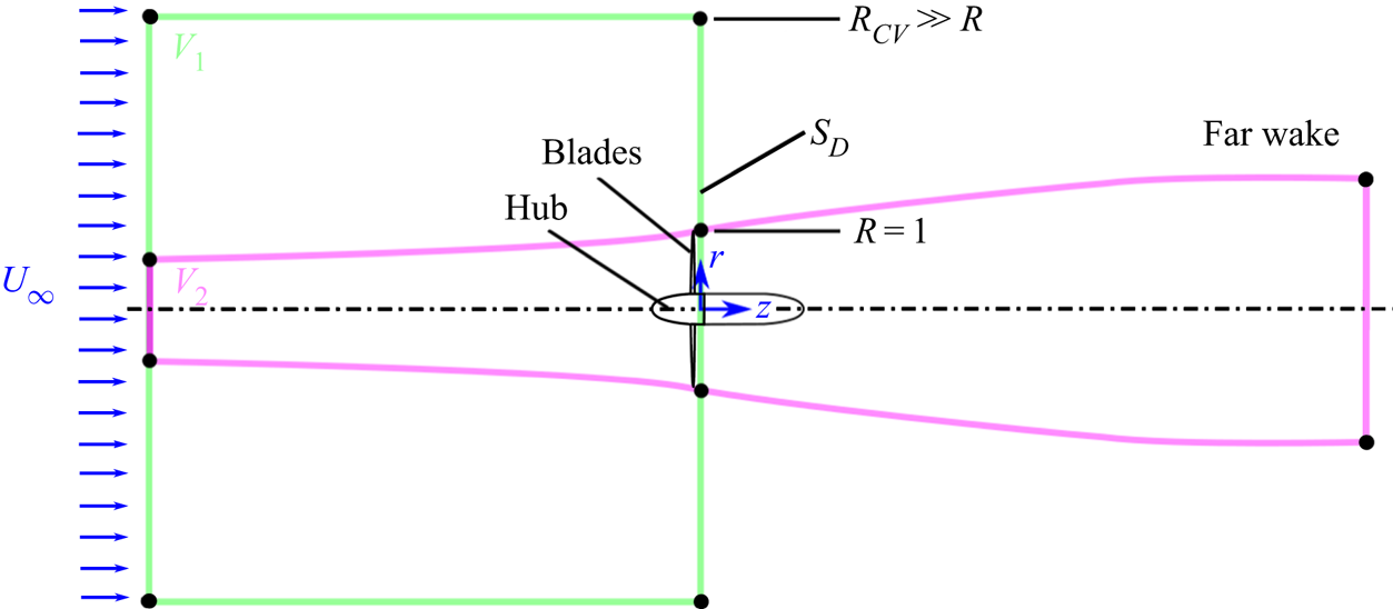
Consider a cylindrical CV encompassing a turbine rotor,  $V_1$, as depicted in figure 1, with one planar face well upstream of the rotor in the undisturbed free stream, and one face just downstream of the rotor,
 $S_D$, where
 $z=0$. The rotor's axis of rotation is colinear with the central axis of the CV, whose radius
 $R_{CV} \rightarrow \infty$, allowing us to assume that the axial velocity on the curved lateral boundary is equal to
 $U_\infty$. Assuming the flow to be incompressible and the flow inside the CV to be steady in a rotor-fixed frame of reference, conservation of mass and momentum in the CV leads to
 \begin{equation} C_T = \frac{1}{\rm \pi} \int_{S_D} \left( 2a(1-a) - p \right) {\rm d}S, \end{equation}
where  $p$ is the normalized gauge pressure.
Control volumes to be referenced in the present work. Here,  $V_1$ is a cylindrical CV of large radius, with its downstream face just behind the blades;
 $S_D$ is the circular downstream face of the bounding control surface of
 $V_1$;
 $V_2$ is a mean streamtube passing through the rotor, extending from the free stream to the far wake where wake expansion is presumed to have ceased.

Typically, this CV definition is not used in axial momentum theory, e.g. Sørensen (Reference Sørensen2016), as there is no obvious and direct way to infer the behaviour of the pressure field on  $S_D$. Instead, the flow is assumed to be circumferentially uniform, i.e.
 $a = a(r)$, and the mean streamtube passing through the rotor and extending from the free stream to the far wake is considered (
 $V_2$ in figure 1). This streamtube is assumed to be of circular cross-section for all
 $z$. It is then assumed that the gauge pressure and radial velocity are zero in the far wake, and that the Bernoulli equation holds on mean streamlines between the near and far wakes. Annular streamtubes – subsets of
 $V_2$ – are all assumed to expand uniformly, allowing us to infer that the axial induction in the far wake is twice that at the rotor; that is, the axial velocity in the far wake (at axial location
 $z = z_{w}$) is taken to be
 $u_z(r_{w},\theta,z_{w}) = 1-2a(r)$, where the locations
 $(r_w,\theta,z_w)$ and
 $(r,\theta,0)$ are connected by a mean streamsurface. These various assumptions allow the removal of pressure from (2.2) and lead to the following classical result:
 \begin{align} C_T &= \frac{1}{\rm \pi} \int_{S_{rot}} 4 a (1-a) \,{\rm d}S \nonumber\\ &= \frac{1}{\rm \pi} \int_0^{2{\rm \pi}} \int_{0}^{1} 4a(1-a) r \,{\rm d}r \,{\rm d}\theta, \end{align}
where  $S_{rot}$ is the swept plane of the rotor, located at
 $z = 0^{-}$ in the chosen coordinate system.
The integrand on the right-hand side of (2.3) is maximized when  $a=0.5$, and when
 $a=0.5$ everywhere on
 $S_{rot}$ we obtain
 $C_T = 1$. As a result, momentum theory cannot account for well-established observations of
 $C_T > 1$, and this high-thrust regime must be modelled empirically in BEM codes, e.g. Buhl (Reference Buhl2005). Although there are second-order modifications to momentum theory to reduce its limitations (for example, one could account for azimuthal velocities in the wake to arrive at what Bontempo & Manna (Reference Bontempo and Manna2017) call ‘generalized momentum theory’, replacing the far-wake zero gauge pressure assumption), the fundamental theoretical issue of high thrust remains unresolved. We are thus motivated to venture an entirely different approach.
2.2. Exact thrust expressions from vortical impulse theory
By applying vortical impulse theory to the CV  $V_1$ in figure 1, Limacher & Wood (Reference Limacher and Wood2021) derived the following expression for the thrust on a steadily rotating turbine in an unbounded, incompressible and steady free-stream flow (neglecting viscous terms on
 $S_D$):
 \begin{equation} C_T = \frac{1}{\rm \pi} \int_{S_D} \{u_\theta^{2} + u_r^{2} - a^{2} - r (1-a) \omega_\theta + r u_\theta \omega_z \} {\rm d}S, \end{equation}
where the two components of vorticity are defined as
 $$\begin{gather} \omega_z = \frac{1}{r} \frac{\partial}{\partial r}\left(r u_\theta\right) - \frac{1}{r} \frac{\partial u_r}{\partial \theta}, \end{gather}$$
 $$\begin{gather}\omega_\theta = \frac{\partial u_r}{\partial z} - \frac{\partial u_z}{\partial r}. \end{gather}$$
The only additional assumption inherent to the derivation of (2.4) is that the flow field within  $V_1$ appears steady in a frame of reference rotating with the blades. It is worth emphasizing that the underlying impulse theory is an exact expression of the conservation of linear momentum, and thus the stated assumptions are rather minor restrictions on the generality of (2.4). For example, no assumption of circumferential uniformity has been made, nor has any circumferential averaging of parameters been implied, in direct contrast to conventional momentum-based analyses. Rather, all parameters in (2.4) through (2.6) are free to vary on
 $S_D$ as functions of
 $r$ and
 $\theta$, i.e. on
 $S_D$ we have
 $u_\theta = u_\theta (r,\theta,0)$,
 $u_r = u_r(r, \theta,0)$, etc.
Although the generality of (2.4) is a virtue of the present approach, we are interested in making simplifications to reveal the conditions under which more well-known expressions from wind turbine theory can be recovered. A key outcome of Limacher & Wood (Reference Limacher and Wood2021) was to present a sufficient set of conditions under which (2.4) collapses to the thrust expression inherent to blade-element theory, wherein the total blade force is taken to be the spanwise integral of the sectional Kutta–Joukowsky force. One of those conditions is that the trailing vorticity be aligned with streamlines on  $S_D$ in the frame of reference rotating with the blades, which may be expected when the flow over the blades remains attached at high Reynolds numbers. This will be the first physical proposition to be considered.
This proposition also happens to solve a practical measurement problem. Using stereo-PIV, all three velocity components on  $S_D$ will be available, but axial velocity gradients will not, and thus the
 $\omega _\theta$-term in (2.4) cannot be resolved. However, when vortex lines and streamlines (in the rotating frame) are aligned on
 $S_D$, we have
 \begin{equation} \frac{u_\theta - \lambda r}{1-a} = \frac{\omega_\theta}{\omega_z}, \end{equation}
where  $\lambda = \varOmega R/U_\infty$ is the tip speed ratio, and
 $\varOmega$ is the dimensional rotation rate of the rotor. This relation allows
 $\omega _\theta$ to be removed from (2.4), yielding
 \begin{equation} C_{T} = \frac{1}{\rm \pi} \int_{S_D} \{ u_r^{2} + u_\theta^{2} - a^{2} + \lambda r^{2} \omega_z \} {\rm d}S, \end{equation}
which can be evaluated using stereo-PIV data on  $S_D$. The validity of this thrust expression, specifically in the high-thrust regime of turbine operation, will be considered in the experimental portion of this work.
As a second proposition, we may simply neglect the  $\partial u_r/\partial z$-contribution to the
 $\omega _\theta$-term in (2.4). Setting
 $\partial u_r/\partial z = 0$ on
 $S_D$ yields
 \begin{equation} C_T = \frac{1}{\rm \pi} \int_{S_D} \left\{u_\theta^{2} + u_r^{2} - a^{2} - r (1-a) \frac{\partial a}{\partial r} + r u_\theta \omega_z \right\} {\rm d}S, \end{equation}
where  $\partial a/\partial r = - \partial u_z/\partial r$ has been substituted. This assumption is plausible at first glance, because one might expect the expansion rate of the mean streamtube passing through the rotor to be maximal at the rotor plane. That is, as Sørensen (Reference Sørensen2016) explains, the rate of streamtube expansion increases as one approaches the rotor from upstream, and decreases as one moves downstream from the rotor towards the non-expanding far wake. However, even for the idealized case of an actuator disk, Sørensen (Reference Sørensen2016) shows that
 $\partial u_r/\partial z$ takes on significant values in the rotor tip region. Whether this has a noteworthy effect on the associated force contribution is a matter for experimental validation.
Since classical thrust expressions do not involve velocity derivatives, we are motivated to manipulate the remaining derivative in (2.9) to remove explicit dependence on  $\partial a/\partial r$, which is achieved by integration by parts. We express the area integral over
 $S_D$ as a double integral over
 $r$ and
 $\theta$, substituting
 ${\rm d}S = r \,{\rm d}r \,{\rm d}\theta$. For the unbounded case, we take the limits on the
 $r$-integral to be
 $0$ to
 $\infty$ and the
 $\partial a/\partial r$-term becomes
 \begin{align} -\int_0^{2{\rm \pi}} \int_0^{\infty} r^{2} (1-a) \frac{\partial a}{\partial r} {\rm d}r\, {\rm d}\theta &= \int_0^{2{\rm \pi}} \left\{ r^{2} a\left. \left(\frac{a}{2} - 1\right) \right|_0^{\infty}\right.\nonumber\\ &\quad \left. + \int_0^{\infty} \left(2a(1-a) + a^{2} \right) r \,{\rm d}r \right\} {\rm d}\theta. \end{align}
The first term inside the  $\theta$-integral on the right-hand side vanishes, since
 $a$ decays rapidly with radius from the edge of the rotor in an unbounded flow (faster than
 $a \propto r^{-2}$). Substituting the remaining terms into (2.9), we obtain
 \begin{equation} C_T = \frac{1}{\rm \pi} \int_{S_D} \{u_\theta^{2} + u_r^{2} + 2a(1-a) + r u_\theta \omega_z \} {\rm d}S. \end{equation}
This result is of clear theoretical interest, as the appearance of the  $2a(1-a)$ term prompts us to ask: Under what conditions will (2.11) reduce to conventional results of momentum theory?
To start, we may note that the  $\omega _z$-term vanishes in the special case of circumferential uniformity (i.e.
 $\partial /\partial \theta \equiv 0$), which is typically assumed in momentum theory. This is shown as follows:
 \begin{equation} \int_{S_D} r u_\theta \omega_z \,{\rm d}S = 2{\rm \pi} \int_0^{\infty} r u_\theta \frac{\partial }{\partial r}(r u_\theta)\,{\rm d}r = \left. {\rm \pi}r^{2} u_\theta^{2} \right|_0^{\infty} = 0. \end{equation}
One obtains the third expression from the second by integration by parts, and the whole expression vanishes because the circulation around any contour outside the wake must be zero. When the flow is not circumferentially uniform, this term cannot be so easily dismissed. In the experiment to be presented, however, it will be evaluated and will be shown to be negligible for the cases considered.
Although the validity of neglecting  $\partial u_r/\partial z$ on
 $S_D$ is yet to be tested, it is less dubious further downstream. Note that (2.9) and (2.11) are both instantiations of our second physical proposition that
 $\partial u_r/\partial z = 0$ on the downstream CS, but nothing in their derivation requires the CS to be directly behind the rotor. If we move it to the far wake and call this new surface
 $S_W$, we can invoke the typical assumption in momentum theory that
 $u_r \equiv 0$ on
 $S_W$, from which
 $\partial u_r/\partial z \equiv 0$ follows. We then obtain
 \begin{equation} C_T = \frac{1}{\rm \pi} \int_{S_W} \{u_\theta^{2} + 2u_z(1-u_z) \} {\rm d}S, \end{equation}
which is identical to what one finds through a conventional momentum balance. The second term is the momentum flux from the large cylindrical CV with  $S_W$ as its downstream CS, and the first term is equivalent to the pressure contribution on
 $S_W$ when wake swirl is considered (McCutchen Reference McCutchen1985; Wood Reference Wood2007).
Our success in recovering a result of a classical momentum balance, expressed in terms of far-wake velocities, corroborates the approach taken thus far. However, we must return our attention to the near wake, with the goal of expressing the thrust in terms of velocities just downstream of the rotor. If we are to recover the familiar  $4a(1-a)$ integrand in (2.3) under some circumstances, we might presume that the
 $\partial u_r/\partial z$-term contribution is, in fact, significant, and that it is of similar magnitude to (and of the same sign as) the
 $\partial a/\partial r$-term in (2.9), from which the
 $2a(1-a)$ term in (2.11) was extracted. This leads us to our third proposition, to be presented in the next subsection.
2.3. A third physical proposition, its thrust expression and a comparison with classical momentum theory
The thrust expressions thus far derived are exact, meaning that the expressions follow directly from the conservation of linear momentum when the corresponding physical propositions strictly hold (alignment of streamlines and vortex lines, or  $\partial u_r/\partial z \rightarrow 0$ on
 $S_D$). The following derivation, based on a third physical proposition, does not attain to quite the same rigour as the first two, and some speculation must be introduced. This third proposition nonetheless warrants consideration, because the resulting thrust expression offers a possible explanation for the high-thrust regime, and it also results in an experimentally based thrust estimate which more closely matches the measured thrust than any other expression thus far presented.
Outside of the wake, we expect the flow to be irrotational, meaning  $\partial u_r/\partial z = -\partial a/\partial r$. We now hypothesize that within the wake the opposite is true, i.e.
 $\partial u_r/\partial z = \partial a/\partial r$. This corresponds to local strain rates of zero, suggesting that the trailing vortex cores are purely ‘rolling’ structures that exhibit no shear. This zero-strain-rate hypothesis is our third physical proposition about the near wake.
Since we are making opposite assertions over different regions of the flow, we must express the transition between them. Let us define  $k(r,\theta )$ as a smooth function such that
 \begin{equation} \omega_\theta = \frac{\partial u_r}{\partial z} + \frac{\partial a}{\partial r} = k(r,\theta) \frac{\partial a}{\partial r}, \end{equation}
everywhere on  $S_D$, and
 $k \in [0,2]$. Where
 $k=0$, the flow is irrotational; where
 $k=2$, the flow is strain-rate free.
The  $\omega _\theta$-contribution in the general thrust equation (2.4) then becomes
 \begin{align} C_{T,\omega_\theta} &={-}\frac{1}{\rm \pi} \int_0^{2{\rm \pi}} \int_0^{\infty} r^{2}(1-a)\omega_\theta \,{\rm d}r \,{\rm d}\theta, \nonumber\\ &={-}\frac{1}{\rm \pi} \int_0^{2{\rm \pi}} \int_0^{\infty} r^{2}(1-a)k \frac{\partial a}{\partial r} {\rm d}r \,{\rm d}\theta. \end{align}
Integrating by parts, the inner  $r$-integral becomes
 \begin{align} -\int_0^{\infty} r^{2}(1-a)\omega_\theta \,{\rm d}r &= \left. -r^{2}a(1-a) \right|_0^{\infty} + \int_0^{\infty} 2 r a(1-a) \,{\rm d}r - \int_0^{\infty} r^{2} k a \frac{\partial a}{\partial r} {\rm d}r \nonumber\\ &\quad + \int_0^{\infty} r^{2} a(1-a)\frac{{\rm d} k}{{\rm d} r} {\rm d}r. \end{align}
The second-last integral can be integrated by parts again, and after algebraic manipulation we obtain
 \begin{align} -\int_0^{\infty} r^{2}(1-a)\omega_\theta \,{\rm d}r &= \left.-r^{2} k a \left( 1 - \frac{a}{2} \right) \right |_0^{\infty} + \int_0^{\infty} ( 2a (1-a) + a^{2} ) r k \,{\rm d}r \nonumber\\ &\quad + \int_0^{\infty} r^{2} a \left(1 - \frac{a}{2} \right) \frac{{\rm d} k}{{\rm d} r} {\rm d}r. \end{align}
The first term on the right-hand side vanishes because the flow is irrotational at infinity; that is,  $k=0$ as
 $r \rightarrow \infty$.
Evaluation of the second and third integrals, however, would require precise knowledge of how the flow transitions from the irrotational to strain-rate-free conditions. In absence of such information, we lean on theoretical expectations to proceed. Our express intention is to recover something which approaches the classical thrust expression in (2.3) for low thrust, but which is capable of yielding thrust estimates in excess of one for highly loaded rotors.
With that aim in mind, let us make the rather simplistic assumption that  $k=2$ everywhere within the wake, and
 $k=0$ everywhere outside it. Defining the radius at the outer edge of the tip vortices to be
 $r = R_e$ – with the expectation that
 $R_e \gtrapprox 1$ – we set
 $k = 2$ when
 $r < R_e$, and
 $k = 0$ when
 $r > R_e$, and assume that
 $k$ varies smoothly between
 $R_e^{-}$ and
 $R_e^{+}$. The second integral in (2.17) then reduces to
 \begin{equation} \int_0^{\infty}
(2a (1-a) + a^{2}) r k \,{\rm d}r = \int_0^{R_e}
(4a (1-a) + 2a^{2}) r \,{\rm d}r,
\end{equation}
recovering the familiar  $4a(1-a)$ term from classical analyses.
The limits on the last integral in (2.17) can changed to be from  $r = R_e^{-}$ to
 $r = R_e^{+}$, because
 $dk/dr = 0$ has been assumed everywhere else. Taking
 $a$ to be constant on
 $R_e^{-} \leqslant r \leqslant R_e^{+}$ (i.e. —
 $\partial a/\partial r| \ll |{\rm d}k/{\rm d}r|$ at
 $r = R_e$),
 $a (1- a/2)$ can be moved out of the integral, which then reduces to
 \begin{equation} \int_{R_e^{-}}^{R_e^{+}} r^{2} a \left(1 - \frac{a}{2} \right) \frac{{\rm d} k}{{\rm d} r} {\rm d}r = R_e^{2} a_e \left( 1 - \frac{a_e}{2} \right)\int_{R_e^{-}}^{R_e^{+}} \frac{{\rm d} k}{{\rm d} r} {\rm d}r ={-} 2 R_e^{2} a_e \left( 1 - \frac{a_e}{2} \right), \end{equation}
where  $a_e = a(R_e, \theta )$. Combining the preceding five equations, we obtain
 \begin{equation} C_{T,\omega_\theta} =
\frac{1}{\rm \pi}\int_0^{2{\rm \pi}} \left\{ \int_0^{R_e} (
4a(1-a) + 2a^{2} ) k r \,{\rm d}r - 2 R_e^{2} a_e
\left( 1 - \frac{a_e}{2} \right) \right\} {\rm d}\theta .
\end{equation}
It is usually assumed that  $a=0$ for
 $r>1$ in classical treatments, and, to proceed, we may assume that
 $a_e = 0$, causing the second term on the right-hand side of (2.20) to vanish. Realistically, the obstruction of the rotor causes some acceleration of fluid beyond the free-stream velocity around the periphery of the swept disk, but this gives a zero crossing of
 $a$ somewhere near the wake's edge, once again making the assumption of
 $a_e = 0$ plausible.
Given the crudeness of the assumption that  $k$ abruptly changes from
 $k=2$ to
 $k=0$, there is little to be gained in arguing about the precise location of
 $R_e$ so as to evaluate
 $a_e = a(R_e,\theta )$. Rather, we will proceed by neglecting the second term in (2.20), satisfied that the form of the resulting expression conforms to our theoretical expectations.
When this is done, and the remaining terms on the right-hand side of (2.20) are substituted for the  $\omega _\theta$-term in (2.4), we obtain
 \begin{align} C_T &= \frac{1}{\rm \pi}
\int_0^{2{\rm \pi}} \int_0^{\infty} \{u_\theta^{2} +
u_r^{2} - a^{2} + r u_\theta \omega_z \} r \,{\rm d}r
\,{\rm d}\theta \nonumber\\ &\quad + \int_0^{2{\rm \pi}}
\int_0^{R_e} \{ 4a(1-a) + 2a^{2}\} r \,{\rm d}r
\,{\rm d}\theta. \end{align}
Having recovered the familiar  $4a(1-a)$ integrand, the squared velocity terms in (2.21) appear as second-order corrections to the classical results of momentum theory, allowing for a thrust coefficient that grows monotonically with increasing
 $a$ and allowing
 $C_T >1$ for
 $a > 0.5$. This is perhaps made clearer if we approximate
 $R_e \approx 1$, and define
 $S_d \subset S_D$ as the projection of the swept rotor plane on
 $S_D$, defined by
 $\theta \in [0, 2{\rm \pi} ]$ and
 $r \in [0,1]$ at
 $z = 0$. Under the assumption that
 $a \approx 0$ for
 $r>1$, we then obtain
 \begin{equation} C_T = \frac{1}{\rm \pi} \int_{S_D} \{u_\theta^{2} + u_r^{2} + a^{2} + r u_\theta \omega_z \} {\rm d}S + \frac{1}{\rm \pi} \int_{S_d} 4a(1-a) \,{\rm d}S. \end{equation}
The classical thrust expression in (2.3) is recovered if the first integral on the right-hand side of (2.22) is neglected. (The integral over  $S_d$ in (2.22), located at
 $z = 0$, is expected to closely approximate the integral over
 $S_{rot}$ in (2.3), located at
 $z = 0^{-}$, as no discontinuity in
 $a$ is expected in the neighbourhood of
 $z=0$.) If valid, (2.22) suggests that momentum theory, and the BEM codes based on it, will underpredict thrust at typical operating values of
 $a$. In fact, underprediction of experimentally measured thrust has been observed for BEM codes across a wide range of tip speed ratios in Krogstad & Eriksen (Reference Krogstad and Eriksen2013).
The novel corrective terms in (2.22) may be interpreted as accounting for wake expansion in a manner not captured by classical momentum theory. The contribution of  $u_r^{2}$ is obviously associated with expansion, but so is the
 $a^{2}$-contribution, since the latter was derived from a term involving
 $\partial u_r/\partial z$.
The various thrust equations derived here in § 2 stand as competing hypotheses. We are unaware of any experiments that have specifically tested their inherent physical assumptions, and neither will we attempt such direct validation in the experimental portion of this work. Rather, we will employ the thrust expressions resulting from each physical proposition, using stereo-PIV data to furnish thrust estimates therefrom, and we will compare those estimates with direct thrust measurements. In this way, we will attempt to corroborate, if not fully validate, at least one of the three physical propositions.
3. Thrust expressions to be applied to the experimental dataset
To summarize the theoretical development in the previous section, three different propositions regarding the near-wake flow field were made. These propositions, and their associated thrust expressions, are as follows:
(i) when we assume that mean streamlines and vortex lines in the near wake are aligned in a frame of reference rotating with the blades, we obtain (2.8);
(ii) when assume that
 $\partial u_r/\partial z \approx 0$ just behind the rotor, we obtain (2.9); and
(iii) when we assume that the trailing vortex cores are rolling structures that exhibit zero-strain rates in their cores, we obtain (2.21).

In an experiment, the flow cannot be resolved out to  $r \rightarrow \infty$, and so the outer bound on the
 $r$-integrals in the three noted equations must be some finite
 $r = R_o$. For the derivations in § 2 to strictly hold, we would strive for
 $R_{o} \gg 1$ such that
 $u_z(R_{o},\theta,0) = U_\infty$. The effect of
 $u_z(R_{o},\theta,0) \neq U_\infty$, either due to insufficiently large
 $R_o$ or due to blockage, is discussed in § 6.2. In the present experiment, there is a limit on the inner radius as well, due to the presence of a central hub. Moreover, the illumination necessary for PIV creates bright near-body reflections that prevent acquisition of accurate velocity data in the vicinity of the hub, so we define the inner radius
 $R_i$ as the innermost location where velocity data can be reliably acquired.
Firstly, a thrust estimate from the classical expression in (2.3) will be acquired according to
 \begin{equation} C_{T,0} = \frac{1}{\rm \pi} \int_0^{2{\rm \pi}} \int_{R_i}^{1} 4a(1-a) r \,{\rm d}r \,{\rm d}\theta. \end{equation}
Our first impulse-based thrust expression for experimental validation, associated with proposition (i), is
 \begin{equation} C_{T,1} = \frac{1}{\rm \pi} \int_0^{2{\rm \pi}} \int_{R_i}^{R_o} \{ u_r^{2} + u_\theta^{2} - a^{2} + \lambda r^{2} \omega_z \} r \,{\rm d}r \,{\rm d}\theta. \end{equation}
Proposition (ii) leads to
 \begin{equation} C_{T,2} = \frac{1}{\rm \pi} \int_0^{2{\rm \pi}} \int_{R_i}^{R_o} \left\{u_\theta^{2} + u_r^{2} - a^{2} - r (1-a) \frac{\partial a}{\partial r} + r u_\theta \omega_z \right\} r \,{\rm d}r \,{\rm d}\theta. \end{equation}
Recall also that this expression was integrated by parts to remove the velocity derivative and arrive at (2.11). For the finite-domain case where we cannot assume  $a = 0$ at
 $r = R_o$, the first
 $\theta$-integral on the right-hand side of (2.10) must not be omitted, and we have a modified version of (2.11)
 \begin{align} C_{T,2a} &= \frac{1}{\rm \pi}
\int_0^{2{\rm \pi}} \int_{R_i}^{R_o} \{u_\theta^{2} +
u_r^{2} + 2a(1-a) + r u_\theta \omega_z \} r \,{\rm
d}r \,{\rm d}\theta \nonumber\\ &\quad + \frac{1}{\rm \pi}
\int_0^{2{\rm \pi}} \left\{ r^{2} a \left.\left(\frac{a}{2} -
1\right) \right|_{R_i}^{R_o} \right\} {\rm
d}\theta, \end{align}
where  $C_{T,2}$ and
 $C_{T,2a}$ incorporate the same physical assumptions, such that when applied to experimental data, they should differ only due to numerical errors in the evaluation of the derivative
 $\partial a/\partial r$. These two expressions will be compared as a check on the sufficiency of the spatial resolution of the acquired velocity field.
Proposition (iii) requires us to make an assumption about where the flow transitions from being strain-rate free to irrotational, and we denoted the radial location of this transition as  $R_e$. The best theoretical agreement with classical momentum theory is obtained when we assume that
 $R_e = 1$, which yields
 \begin{align} C_{T,3} &= \frac{1}{\rm \pi}
\int_0^{2{\rm \pi}} \int_{R_i}^{R_o} \{u_\theta^{2} +
u_r^{2} - a^{2} + r u_\theta \omega_z \} r \,{\rm d}r
\,{\rm d}\theta \nonumber\\ &\quad +
\frac{1}{\rm \pi}\int_0^{2{\rm \pi}} \int_{R_i}^{1} \{ 4a(1-a)
+ 2a^{2} \} r \,{\rm d}r \,{\rm d}\theta.
\end{align}
In the experimental data to be presented below, collected at a small distance downstream of the rotor, the tip vortices can be observed to extend beyond  $r=1$, and
 $R_e = 1$ might be called into question. To show that this choice has a small effect on the thrust estimates, we define an alternative expression in which we set
 $R_e = R_o$, at the outer edge of the domain to be observed. Changing the upper limit on the second
 $r$-integral in (3.5) from
 $r=1$ to
 $r = R_o$, the two integrals can be combined to yield
 \begin{equation} C_{T,3a} = \frac{1}{\rm \pi} \int_0^{2{\rm \pi}} \int_{R_i}^{R_o} \{u_\theta^{2} + u_r^{2} + a^{2} + r u_\theta \omega_z + 4a(1-a) \} r \,{\rm d}r \,{\rm d}\theta. \end{equation}
4. Methodology
4.1. Experimental apparatus
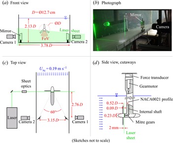
A stereo-PIV investigation on a stream-normal plane just behind a turbine rotor was undertaken in a water channel facility at Princeton University. Figure 2 shows top-, front- and side-view sketches and a photograph of the experimental set-up. The illuminated plane was  $0.09D$ behind the trailing edge of the turbine blades, where
 $D = 127$ mm is the turbine diameter. This was judged to be as close as practically possible without encountering severe reflections from the blades in the acquired images.
Experimental set-up; (a) front-view sketch, showing the FoV for stereo-PIV data capture; (b) photograph of the set-up, showing the laser sheet intersecting the transparent hub just behind the blades; (c) top-view sketch, showing arrangement of mirrors and cameras, and the  $60^{\circ }$ angle between the cameras’ optical axes; (d) side view with cutaways, showing internal shafts driving the rotor, and showing the mounting of the gearmotor and force transducer above the waterline. Sketches are not to scale.

The sampled field of view (FoV) is below the axis of the rotor where both cameras have optical access, as shown in figure 2. Individual sectors of the velocity field are measured sequentially, and a complete  $360^{\circ }$ velocity field is reconstructed using the stitching method described in § 4.5.
A Litron NANO L50-50PIV dual-pulse laser was used for illumination, with the beam manipulated into a  $2$ mm-thick sheet using standard sheet optics. Two LaVision sCMOS CLHS cameras were mounted about
 $2.76D$ downstream of the illuminated plane, oriented with their viewing axes normal to the acrylic channel walls to prevent optical distortion. The viewing axes were redirected upstream using
 $76$ mm square mirrors mounted inside the channel, achieving a
 $60^{\circ }$ angle between the two views. Image capture and laser firing were synchronized using a LaVision PTU X programmable timing unit. Particle image-pair acquisition was triggered once per rotation based on the motor encoder signal using a programmable OSOYOO Due R3 microcontroller. The flow was seeded with silver-coated hollow glass spheres of mean diameter
 $14\ \mathrm {\mu }{\rm m}$ (Potters Industries, S5000-S3).
The rotor was driven by a gearmotor with a 3.7 : 1 gear ratio (Phidgets 3265_0) mounted above the waterline using shafts internal to the supporting apparatus. This apparatus consisted of a cylindrical fuselage ( $0.23D$ in diameter) with an elliptical aft body, and a vertical sting with an airfoil cross-section (NACA0024 near the fuselage, transitioning to a NACA0021 profile above) whose chord length was
 $60$ mm, or
 $0.47D$. Both the fuselage and the sting, as well as auxiliary mounting components above the waterline, were fabricated using the fusion deposition modelling (FDM) method of three-dimensional (3-D) printing.
The investigated turbine rotor is modelled after that of McTavish, Feszty & Nitzsche (Reference McTavish, Feszty and Nitzsche2014), which they designed specifically for the low-Reynolds-number environment of a water channel. In the present study, the rotor hub diameter has been increased from their value of  $0.1D$ to
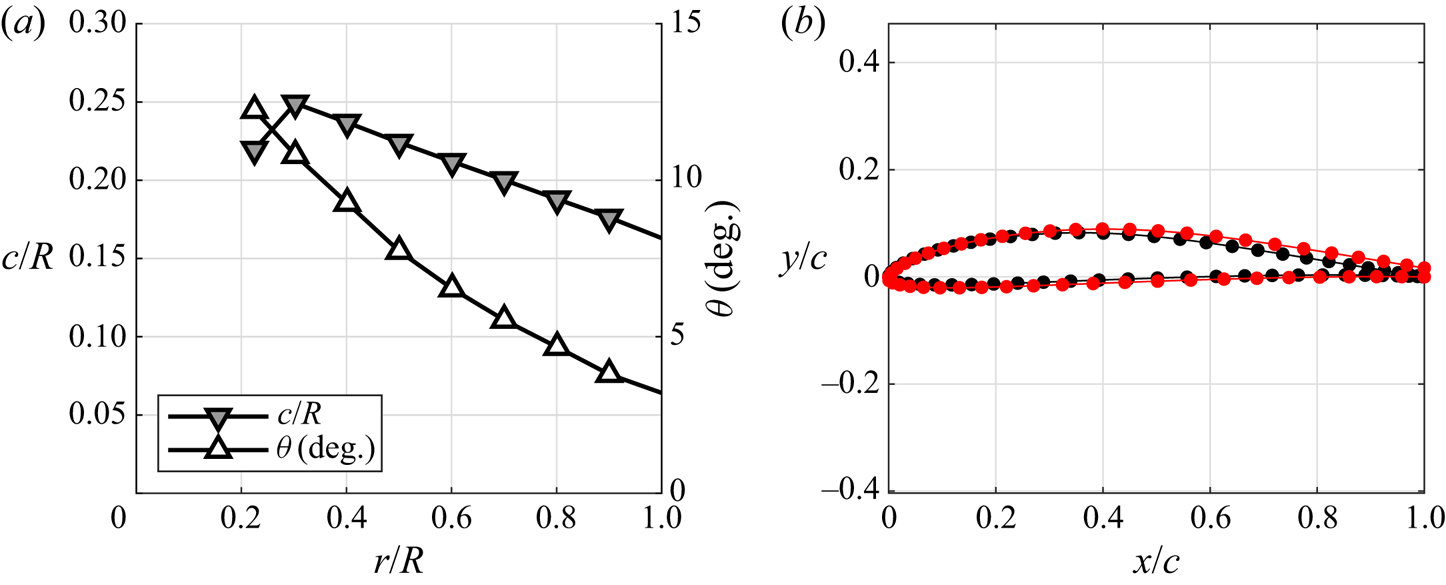
 $0.23D$ to accommodate the internal components needed to drive the rotor. The chord and twist distributions of the blades are shown in figure 3(a).
(a) Chord and twist distributions –  $c/R$ and
 $\theta$, respectively – of the rotor blades; (b) standard Eppler E387 airfoil cross-section (black markers) and the modified E387 airfoil with a trailing edge of finite thickness (red markers), truncated for ease of manufacture by 3-D printing.

The rotor was fabricated using the stereolithography apparatus method of 3-D printing to achieve a smoother surface finish than is possible using FDM. The three blades and the hub were printed separately and then friction-fit together. A polymer known by the tradename WaterShed 11122XC was chosen for its translucence to minimize reflections at the surface that may saturate particle images and prevent the acquisition of adequate particle-image correlations near the hub and blades. A modified Eppler E387 airfoil cross-section was used for the blades, where the trailing edge has been truncated to have sufficient thickness for 3-D printing. The modified airfoil cross-section is shown in figure 3(b) alongside the standard Eppler E387 airfoil, as obtained from the online airfoil database maintained by the Applied Aerodynamics Group at University of Illinois at Urbana-Champaign (UIUC). (https://m-selig.ae.illinois.edu/ads/coord_database.html.)
The entire rotor, fuselage and sting assembly was mounted to a six-axis force transducer (ATI Mini40) above the waterline, which itself was rigidly mounted to the water channel frame.
4.2. Motor control
In the present work, tip speed ratios of  $\lambda = \{4.37, 5.25, 6.12, 7.00, 7.87, 8.75, 9.62, 10.50\}$ were investigated. The free-steam velocity was held fixed at
 $U_\infty = 0.19\ {\rm m}\ {\rm s}^{-1}$ for all tip speed ratios and the rotor speed was set to
 $\varOmega = \{125, 150, 175, 200, 225, 250, 275, 300\}$ r.p.m.
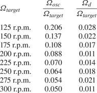
The gearmotor speed was controlled using closed-loop feedback of an encoder signal (Anaheim Automation ENC-A4TS-0360-197-H-M). Extant motor speed variations can be characterized as the superposition of an oscillation at the rotor frequency, possibly caused by uneven friction in the drivetrain, and a non-stationary slow drift. This superposition can be expressed as
 \begin{equation} \varOmega = \varOmega_{target} + \varOmega_{osc} \sin (2{\rm \pi} f_{rot} t) \pm \varOmega_d, \end{equation}
where  $\varOmega _{target}$ is the target speed,
 $\varOmega _{osc}$ is the oscillating component at the frequency of rotation, and
 $\varOmega _d$ is treated as a random error due to the slow drift.
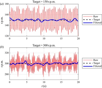
Examples of the r.p.m. signals acquired by numerical differentiation of the encoder signal (using the method of central differences) are shown as red lines in figure 4(a) and 4(b). Applying a modified-Gaussian low-pass filter, as defined in Limacher et al. (Reference Limacher, Morton and Wood2019), with passband and stopband frequencies of  $0.2f_{rot}$ and
 $0.3f_{rot}$, we obtain estimates of the slow drift, shown as blue lines on the same figure.
Examples of the motor-speed signal, acquired by numerical differentiation of the raw encoder signal. The red lines are the raw signals, the dashed black lines are the target r.p.m., and the blue lines are the low-pass filtered signal highlighting the non-stationary long-term drift: (a) 150 r.p.m. target; (b) 300 r.p.m. target.

Calculating the standard deviation of the r.p.m. signal over ten rotor cycles,  $\sigma _{10cyc}$, we estimate the oscillatory amplitude as
 $\varOmega _{osc} = \sqrt {2} \sigma _{10cyc}$, and the instantaneous uncertainty associated with the long-term drift is characterized as twice the standard deviation of the low-pass filtered signal over a 20 s sample. Values of
 $\varOmega _{osc}$ and
 $\varOmega _d$ are reported in table 1.
Characterization of the motor-speed variability. Here,  $\varOmega _{osc}$ represents the amplitude of the oscillatory component at the frequency of rotation;
 $\varOmega _d$ represents the instantaneous uncertainty associated with the non-stationary slow drift of the mean motor speed.

4.3. Direct force measurements
The measured rotor thrusts were small, amounting to approximately  $0.2N$ for a thrust coefficient of
 $C_T = 1$. This is at the low end of the
 $0N$ to
 $20N$ measurement range of the ATI Mini40 force transducer, and it was deemed necessary to perform an in-house calibration over the range from
 $0N$ to
 $0.4N$. In addition, to obtain repeatable results, it was found necessary to apply a constant pre-load in the downstream direction of a few Newtons using an elastic band. Unrepeatable results in absence of this preload were attributed to static friction internal to the transducer. Over this range of forces, linear regression revealed a linearity error of about
 $0.6\,\%$, and a zero-offset error of
 $0.0008N$. This value is less than the measurement resolution of
 $0.005N$, indicating that the zero offset is effectively zero. After normalization, the thrust coefficient resolution is
 $0.022$.
Another challenge to the use of the Mini40 transducer is the non-stationary drift in the signal over long times. Leaving the unloaded transducer over 30 minutes, this drift could be as high as  $0.05N$, which is significant for our purposes. Only relative changes in thrust over short times were deemed trustworthy. To address this challenge, we performed two types of thrust test. In the first, which we call a ‘ramp-up test’, we started recording thrust with the water channel and the rotor off; after 45 s, we ramped up the water channel speed to
 $0.19\ {\rm m}\ {\rm s}^{-1}$ and turned the rotor on at
 $\varOmega = 250$ r.p.m.; taking the mean thrust over at least 25 s, and repeating this test four times, we established a repeatable reference thrust,
 $T_{250}$, for subsequent trials. To determine the thrust at all other rotor speeds, we began trials with the channel on and the rotor at
 $250$ r.p.m., then changed the rotor set point to the new desired value and measured the change in mean thrust,
 $\Delta T_\varOmega$, allowing the thrust at each speed to be calculated as
 $T_\varOmega = T_{250} + \Delta T_\varOmega$. Due to this summation, the zero-order uncertainty due to sensor resolution is increased by a factor of
 $\sqrt {2}$ (Moffat Reference Moffat1988), resulting in an uncertainty contribution of
 $\delta C_{T,a} = 0.031$ in the thrust coefficients. In the reported results, this uncertainty will be added to two standard deviations of individual thrust measurements to yield a total uncertainty estimate.
Ten repeated trials for each rotor speed were conducted, five of which were conducted after the rotor apparatus was disassembled and reassembled. The thrust on the fuselage and sting were also characterized using five ramp-up tests with a bladeless rotor (a hub only), and this thrust has been subtracted from all measured thrust values to give the measured rotor thrust coefficients reported in § 5.
All force data were acquired at a sampling rate of  $200$ Hz.
4.4. The PIV methodology
For each sector, 200 image pairs were captured with both cameras, with an interframe time of  $2$ ms. Mean velocity fields were calculated from particle-image pairs in LaVision's DaVis 10 software using the sum-of-correlations method (Meinhart, Wereley & Santiago Reference Meinhart, Wereley and Santiago2000), wherein all 200 cross-correlation maps are averaged before the correlation peak is identified and used to calculate velocity. This method reduces random error in the calculated mean velocities by effectively weighting sharper correlation peaks more strongly. By contrast, if each correlation map were used to calculate a particle displacement and these displacements were averaged, a single erroneous vector from a diffuse correlation peak could greatly skew the mean value.
By using 200 correlation maps ( $N = 200$) to compute the mean velocity field, the uncertainty in local mean velocity components is made acceptably low. If instantaneous deviations from the true mean (whether physical or spurious) are normally distributed with a standard deviation of
 $\sigma$, then repeated experiments would yield calculated means with a standard deviation about the true mean of
 $\sigma /\sqrt {N}$ (Moffat Reference Moffat1988) – in this case,
 $0.07 \sigma$ – and we may presume the error in our measured mean velocities to be of the order of
 $1\,\%$. When those velocity data are used as inputs to the thrust expressions given in § 3, the integration operations reduce uncertainty in the thrust estimates even further and this source of error can be neglected.
PIV calibration was performed using a 3-D calibration plate (LaVision 106-10), with  $2.2$ mm-diameter marks separated by
 $10$ mm on each plane, and the two planes separated by
 $2$ mm. The calibration was refined using the planar self-calibration function in LaVision DaVis 10 (Wieneke Reference Wieneke2005), applied on over
 $900$ particle-image pairs for the free-stream flow with the experimental apparatus removed. The mean free-stream velocity of
 $U_\infty = 0.19\ {\rm m}\ {\rm s}^{-1}$ was also obtained from this dataset.
To correct for variations in laser sheet brightness over the field of view, each image underwent local brightness normalization over a  $300$ pixel region. The brightness of the second image of each image pair was normalized to the brightness of the first to correct for any difference in energy between the two laser pulses. A min/max filter over a length of four pixels was also applied.
Multi-pass correlations were employed, performing one pass with a window size of  $64 \times 64$ pixels and
 $50\,\%$ overlap, and a second pass with
 $32 \times 32$ pixels and
 $75\,\%$ overlap. The resulting vectors are spaced in the
 $x$- and
 $y$-directions by
 $0.00655R$.
In vector post-processing, vectors with a correlation value of less than  $0.5$ were removed. Universal outlier detection (Westerweel & Scarano Reference Westerweel and Scarano2005) was also employed on
 $5 \times 5$ vector regions to remove spurious vectors. Vectors rejected in these ways were replaced by interpolation. No additional smoothing was applied, as Limacher et al. (Reference Limacher, McClure, Yarusevych and Morton2020) found that even modest spatial filtering can cause impulse-based force expressions to underestimate drag.
4.5. Velocity field processing
As shown in figure 2, only the lower portion of the rotor is visible to both cameras, allowing a  $36^{\circ }$-sector with an outer radius of
 $1.2R$ to be captured at any given moment. To reconstruct the complete
 $360^{\circ }$ flow field, 15 of these sectors were captured, each separated by
 $24^{\circ }$ from its neighbours, yielding
 $12^{\circ }$ of overlap on either side of each sector. In the reconstruction, the velocity fields in the overlapping regions were taken as a linearly varying weighted average of the two adjacent sectors.
For ease of plotting and thrust calculations, the PIV data, acquired on a Cartesian grid, are linearly interpolated onto a circular grid, with equal radial and angular spacing of  $\Delta r = 0.0039R$ and
 $\Delta \theta = 0.0031$ rad between data points. Using these stitched and interpolated velocity fields, the equations presented in § 3 will be used to estimate thrust. In all of those equations, the integrand takes the form
 $r f(r,\theta )$, and the integrals will be approximated using a midpoint integration method
 \begin{equation} \int_0^{2{\rm \pi}} \int_{r_1}^{r_2} f(r,\theta) r \,{\rm d}r \,{\rm d}\theta \approx \Delta \theta \Delta r \sum_i \sum_j f_{ij} r_{ij}. \end{equation}
Although the turbine extracts energy from the flow for most of the investigated tip speed ratios, its rotation is driven by a motor. This is made possible by the small magnitude of power extracted, which is readily dissipated by the friction of the drivetrain, or by the electrical resistance internal to the motor. To confirm that the system extracts positive energy over at least some of the investigated tip speed ratio range, we will calculate the power coefficient,  $C_P$, using the near-wake velocity data. Applying the conservation of angular momentum to the volume
 $V_1$, and calculating power as torque multiplied by rotational speed, we obtain
 \begin{equation} C_P ={-}\frac{2\lambda}{\rm \pi} \int_0^{2{\rm \pi}} \int_{R_i}^{R_{CV}} (1-a)u_\theta r^{2} \,{\rm d}r \,{\rm d}\theta, \end{equation}
which is numerically approximated using discrete data according to (4.2). The calculated  $C_P$ curve serves as a check on the reasonability of the velocity data, and we can verify that the measured thrust curve is consistent with the power regime in which the rotor operates.
Where the laser sheet intersects the translucent rotor hub, the background brightness in the images is significant. To avoid biased correlations that will introduce error into the calculations of force and power, all data within  $r \leqslant R_i = 0.28 R$ will be omitted.
5. Results
5.1. Velocity fields
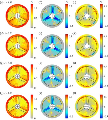
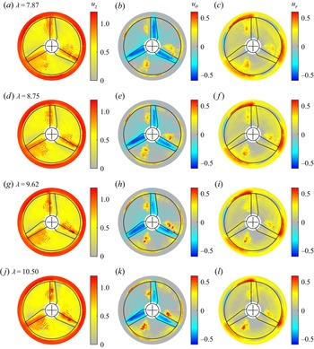
Figures 5 and 6 show the three components of the acquired velocity fields for each of the eight different tip speed ratios. Rotor rotation is counterclockwise in these plots. The axial and azimuthal velocity plots show patterns consistent with the presence of three blades just upstream of the investigated plane, featuring: accelerated axial flow ahead of the blades; a notable velocity deficit aft of the blades; and pronounced azimuthal velocity directly downstream of the blades. These observations are consistent with the expected sense of the bound blade circulation. Extrema in the radial velocity magnitude occur around the periphery of the swept disk, including both inward and outward velocity peaks. These features are consistent with the formation of tip vortices, and their changing blade-relative position with increasing tip speed ratio is consistent with decreasing helical vortex pitch.
Three components of the velocity field in the near wake of the turbine for tip speed ratios of  $4.37$,
 $5.25$,
 $6.12$ and
 $7.00$, arranged in rows from top to bottom. (a,d,g,j) Axial velocity fields; (b,e,h,k) azimuthal velocity fields; (c, f,i,l) radial velocity fields. Blade rotation is counterclockwise, as are positive azimuthal velocities. Positive radial velocities are directed outwards. The outline of the normal projection of the blades onto the interrogated plane, and the circle traced by the tips at
 $r = 1$, are shown in black on each panel.

Three components of the velocity field in the near wake of the turbine for tip speed ratios of  $7.87$,
 $8.75$,
 $9.62$ and
 $10.50$, arranged in rows from top to bottom. (a,d,g,j) Axial velocity fields; (b,e,h,k) azimuthal velocity fields; (c, f,i,l) radial velocity fields. Blade rotation is counterclockwise, as are positive azimuthal velocities. Positive radial velocities are directed outwards. The outline of the normal projection of the blades onto the interrogated plane, and the circle traced by the tips at
 $r = 1$, are shown in black on each panel.

Other less expected features include an oscillatory pattern in the axial velocity field in the region ahead of the blades. The persistence of this feature through the averaging of 200 PIV correlation maps suggests that it is repeatable, and may be attributed to mechanical vibrations of the structural apparatus at an integer multiple of the rotational frequency.
In roughly the same regions, significant positive azimuthal velocity and outwards radial velocity is also observed. The spatial arrangement of these features most clearly shows the mild circumferential flow asymmetries in the mean fields that arise due to temporal variability of the motor speed, as discussed above in § 4.2. These features cannot be dismissed as measurement errors. They are clearly not random errors, as they persist through phase averaging. They also cannot be due to optical distortions in, for example, the acrylic walls of the water channel, because they do not appear in every sampled sector from which the stitched fields were reconstructed.
We will now demonstrate that these unexpected features do not affect our conclusions regarding the validity of our three propositions. However, it is important to consider their origin. In particular, the in-plane velocity features could be physically explained by the presence of a streamwise vortex generated by the pump that drives the flow. When no flow conditioning is applied, such a vortex is clearly observable spanning the length of the water channel, but it is not readily apparent when a honeycomb and flow screens are placed in the plenum upstream of the test section. If a less coherent vortex remains after flow conditioning, it may have escaped detection in the free-stream flow characterization due to a tendency to wander spatially. With a steadily operating rotor present, this hypothetical vortical feature may be driven to oscillate more regularly, generating artifacts that survive phase averaging of the velocity field.
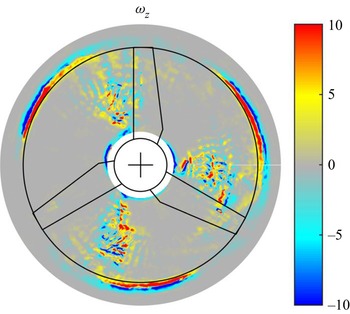
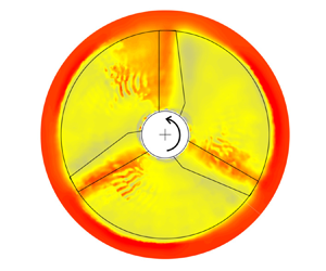
A sample contour plot of  $\omega _z$ at
 $\lambda = 7$, shown in figure 7, exhibits a speckled pattern in the same region as the observed velocity artifacts. This pattern is reminiscent of characteristic random noise in instantaneous PIV-acquired vorticity fields, but should not be attributed to random error in this case because it is not consistent throughout the domain. Rather, this pattern suggests relatively high local turbulence intensities around the observed anomalies, consistent with the presence of an incoherent streamwise vortex. The regions of highest vorticity magnitude are found near the periphery of the swept disk.
Contour plot of vorticity for  $\lambda = 7.87$.

Assuming the anomalous flow features to be physical, it is necessary to consider their effect on the thrust estimates to be presented in § 5.3. In § 5.4, the contributions of individual terms in the thrust expressions are presented, and it is demonstrated that these flow features do not affect the conclusions to be drawn.
5.2. Power coefficients
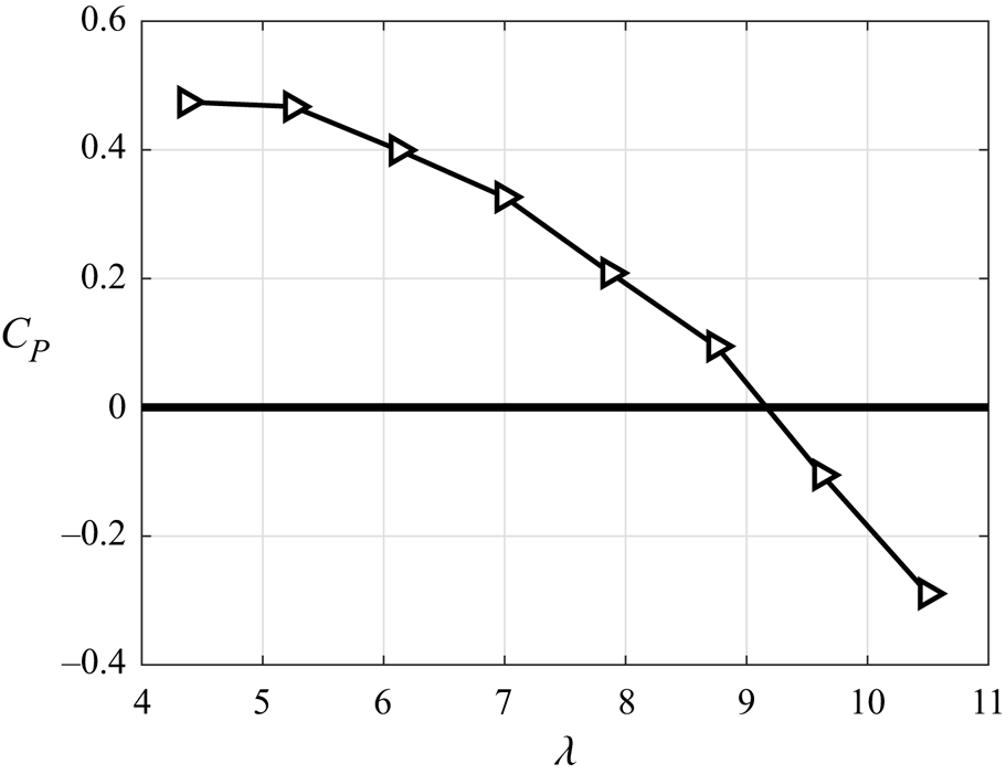
The power coefficient, calculated using (4.3), is plotted vs tip speed ratio in figure 8, with peak performance occurring at the lowest investigated tip speed ratio of  $4.37$. The maximum
 $C_{P,max} = 0.474$ seems impressive for a turbine operating at a diameter-based Reynolds number of
 $Re = DU_\infty /\nu = 1.23 \times 10^{4}$ (where
 $\nu$ is kinematic viscosity), but recall that this rotor was designed specifically for small water channel environments (McTavish et al. Reference McTavish, Feszty and Nitzsche2014). By interpolation, the natural runaway condition of this rotor (where
 $C_P = 0$) is at a tip speed ratio just above nine, and energy must be put into the flow to drive the rotation at the two highest tip speed ratios under investigation.
Power coefficient,  $C_P$, as calculated using (4.3), vs tip speed ratio,
 $\lambda$. The rotor reaches its runaway condition at a tip speed ratio just above
 $9.0$, above which energy must be put into the flow to drive the rotation.

5.3. Measured and calculated thrust coefficients
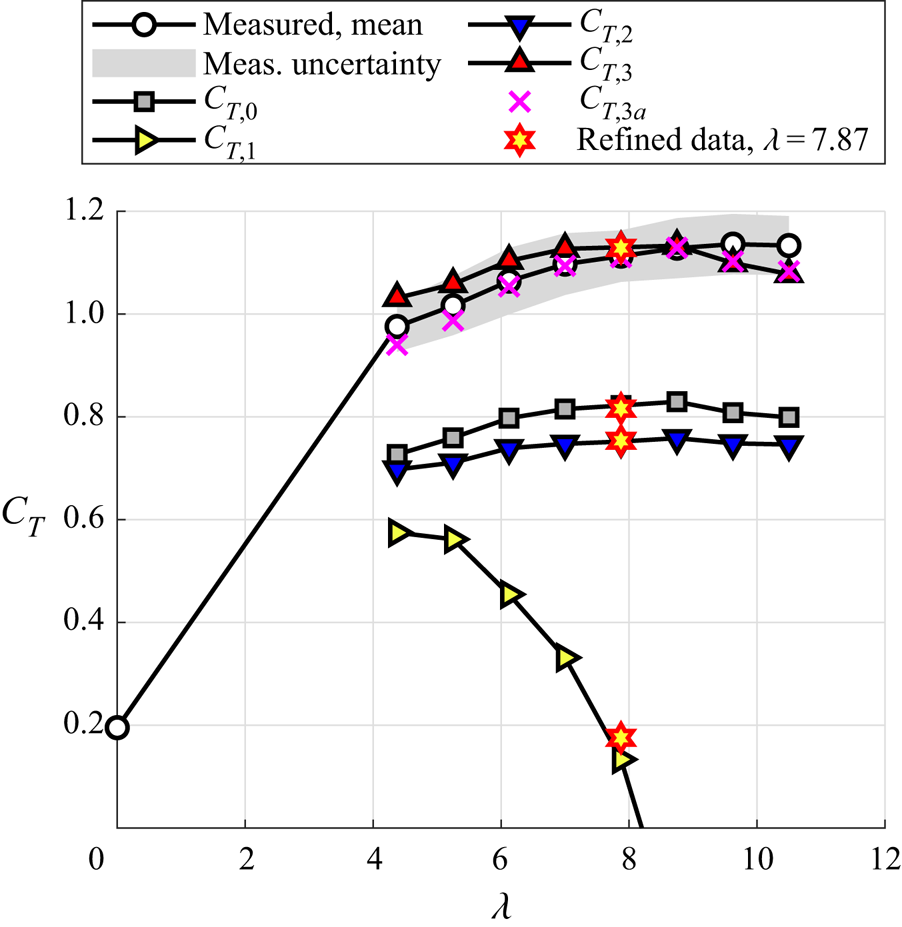
The measured and calculated thrust coefficients are plotted together in figure 9. The narrow grey band around the mean measurements denotes an estimate of uncertainty, defined here as twice the standard deviation of the individual measurements at each tip speed ratio, plus the zero-order uncertainty associated with the force sensor resolution. The trend of gently increasing  $C_T$, with a magnitude just above unity, is consistent with a turbine operating on the so-called ‘backside’ of the curve, i.e. at tip speed ratios between the power optimum and the runaway condition, e.g. Krogstad & Adaramola (Reference Krogstad and Adaramola2011).
Comparison of measured and calculated thrust using (3.1), (3.2), (3.3), (3.5) and (3.6), denoted as  $C_{T,0}$,
 $C_{T,1}$,
 $C_{T,2}$,
 $C_{T,3}$ and
 $C_{T,3a}$, respectively, plotted vs tip speed ratio,
 $\lambda$. The estimates furnished by (3.4) – denoted as
 $C_{T,2a}$ in the text – have not been shown here, because they differ from
 $C_{T,2}$ by
 ${<}0.1\,\%$ for all
 $\lambda$. The thrust estimates labelled as ‘refined data’ (yellow-filled red stars) for
 $\lambda = 7.87$ were calculated from reprocessed PIV data using
 $16\times 16$ windows instead of
 $32 \times 32$. There is one refined-data marker for each of the four thrust expressions
 $C_{T,0}$ through
 $C_{T,3}$; these markers overlap closely with the corresponding data points in the thrust curves calculated with the original data, showing the minimal effect of improved spatial resolution.

The classical thrust expression from momentum theory underpredicts the mean measured thrust curve by  $25\,\%$ to
 $30\,\%$, averaging
 $28\,\%$. Such underprediction is expected for a turbine operating above its optimal tip speed ratio. Recall that, for any value of
 $a$, it is impossible to attain
 $C_T > 1$ from (3.1), and the rectification of this shortcoming of momentum theory is an ultimate aim of this work.
The first impulse-based thrust estimate,  $C_{T,1}$, yields the poorest estimate of all those presented. It drastically underpredicts the measured thrust magnitude, and fails even to capture the thrust trend. The trend is, however, remarkably similar to the trend of
 $C_P$ vs
 $\lambda$ in figure 7. This observation might indicate that the derivation of
 $C_{T,1}$ contains an implicit assumption about the relationship between thrust and useful work, as discussed further in § 6.3.
 $C_{T,2}$ from (3.3) captures the measured thrust trend, but underpredicts its magnitude by
 $31\,\%$ to
 $35\,\%$, with an average of
 $33\,\%$ across tip speed ratios. Equation (3.3) contains a term dependent on
 $\partial a/\partial r$, and we must consider whether the observed thrust underprediction is due to a failure to capture this gradient accurately. In (3.4), this derivative term has been removed by integration by parts, and the resulting estimate – denoted as
 $C_{T,2a}$ in (3.4) – differs from
 $C_{T,2}$ by
 ${<}0.1\,\%$ for all
 $\lambda$. This similarity suggests that the data's spatial resolution is sufficient to avoid numerical errors in the derivative estimate. Since
 $C_{T,2a}$ would be indistinguishable from
 $C_{T,2}$ on figure 9, the former has been omitted for clarity.
One further check on the spatial resolution has been undertaken. The stereo-PIV data were reprocessed using a final window size of  $16 \times 16$ pixels instead of
 $32 \times 32$, again with
 $75\,\%$ overlap, halving the spacing between neighbouring vectors. This was done for only one tip peed ratio,
 $\lambda = 7.87$, and the results are plotted as yellow-filled red stars in figure 9. There is one marker for each of the four thrust expressions,
 $C_{T,0}$ through
 $C_{T,3}$, and these markers overlap closely with the corresponding data points in the thrust curves calculated with the original data, again corroborating the sufficiency of the spatial resolution.
The value of  $C_{T,3}$ shows good agreement with the measured thrust curve in figure 9, differing from it by
 $5.7\,\%$ at worst. Given the approximations that were made, the observed agreement cannot serve as an unequivocal validation of the inherent physical hypothesis, but it certainly affirms the consideration of strain rates in trailing vortex cores as worthy of further consideration. Also,
 $C_{T,3a}$ differs from
 $C_{T,3}$ only in terms of where the abrupt transition between the assumed strain-rate-free and irrotational conditions occurs: the transition is taken to lie at
 $r = R_o = 1.2$ in
 $C_{T,3a}$, and at
 $r = 1$ in
 $C_{T,3}$. This choice has only a small impact on the resulting force estimates, and
 $C_{T,3a}$ is also in good agreement with the measured thrust coefficients across all
 $\lambda$.
5.4. Individual thrust contributions and error sensitivity
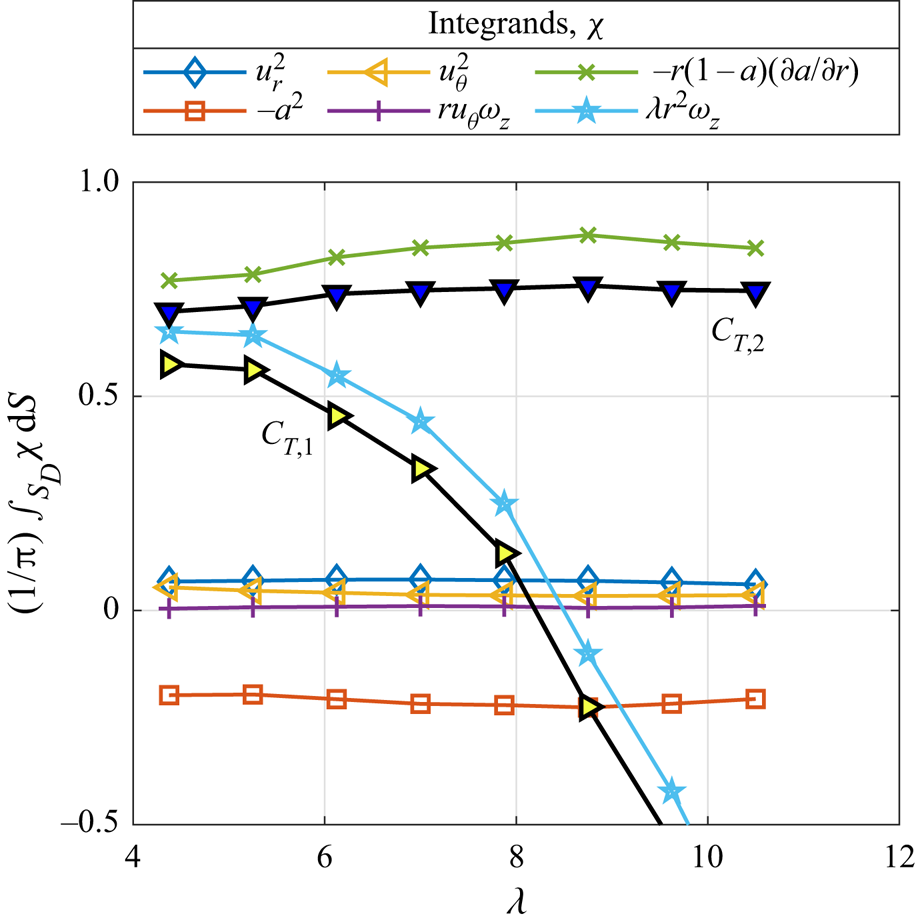
The individual contributions of each term in (3.2) and (3.3) are plotted in figure 10, to help give a better understanding of the reasons for the observed discrepancies between the measured thrust coefficients and  $C_{T,1}$ and
 $C_{T,2}$. The squared velocity contributions are common to both equations. Of these, only the
 $-a^{2}$-contributions are of significant magnitude, varying between
 $-0.21$ and
 $-0.24$, whereas the
 $u_r^{2}$ contributions have a mean value of
 $0.068$. The
 $u_\theta ^{2}$-contribution is lesser still. Although it is not apparent due its small magnitude, the
 $u_\theta ^{2}$-contribution does decrease with increasing tip speed ratio as expected.


The  $r u_\theta \omega _z$-contribution is also small, despite significant circumferential velocity magnitudes directly behind the blades, as seen in figures 5 and 6. This is explained by the relatively low vorticity magnitudes in the same areas, as shown for
 $\lambda = 7.87$ in figure 7.
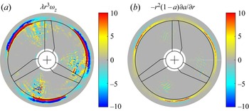
For  $\lambda = 7.87$, figures 11(a) and 11(b) present the spatial distribution of contributions to the vortical terms for
 $C_{T1}$ and
 $C_{T2}$ –
 $\lambda r^{3} \omega _z$ and
 $-r^{2} a (\partial a/\partial r)$, respectively, where the integrands given in the legend of figure 10 have been multiplied by
 $r$ because
 ${\rm d}S = r \,{\rm d}r \,{\rm d}\theta$. Both
 $C_{T1}$ and
 $C_{T2}$ are dominated by their vortical terms, which in turn are dominated by contributions around the periphery of the swept disk. The ‘speckled’ regions ahead of the blades in figure 11(a), which are observable for all
 $\lambda$, are amplifications of the speckled pattern in the vorticity plot in figure 7. However, the contribution of the region within
 $r < 0.95$ to
 $C_{T,1}$ is always positive, so omitting the anomalous features would only worsen the thrust estimates. Figure 11(b) shows that the vortical component of
 $C_{T,2}$ is not as sensitive as
 $C_{T,1}$ to the anomalous flow features ahead of the blades, and the magnitude of the contribution within
 $r < 0.95$ is
 $< 0.1$ for all
 $\lambda$. Thus, we conclude that anomalous flow features in figures 5, 6, and 7 are not to blame for the discrepancies between measured and calculated thrusts.


The dominance of the vortical term's contribution to  $C_{T,1}$ raises the issue of error sensitivity. The derivation of
 $C_{T,1}$ attempts to capture the dynamic effect of both
 $\omega _\theta$ and
 $\omega _z$ in one expression dependent on the latter, but at these tip speed ratios – if vortex lines and streamlines are really coincident – the helical pitch of the wake would be short, and
 $\omega _\theta$ would be the greater component of vorticity. Thus, by using (3.2), we are attempting to estimate a large quantity by multiplying (by a large factor) a smaller quantity that is prone to high uncertainties when acquired using PIV. Although this is plausible, we discuss in § 6.3 why a physical explanation remains more likely.
We likewise conclude that the inaccuracy of  $C_{T,2}$ is due to the inadequacy of the physical assumption that underlies it, since we have already demonstrated that the spatial resolution was sufficient to avoid errors in the numerical evaluation of the derivative
 $\partial a/\partial r$.
Indeed, we must note that the physical assumptions inherent to  $C_{T,2}$ and
 $C_{T,3}$ are mutually exclusive – either the
 $\partial u_r/\partial z$-term is negligible, or it is not. The fact that
 $C_{T,3}$ performs so well suggests that it is not, in fact negligible. This failure was foreshadowed, if not outright predicted, from the manipulation of
 $C_{T,2}$ that led to the expression for
 $C_{T,2a}$ in (3.4). The appearance of the
 $2a(1-a)$ integrand in that equation hinted that the neglect of the
 $\partial u_r/\partial z$-term might leave us incapable of recovering the classical
 $4a(1-a)$ integrand under typical operating conditions – conditions for which classical expressions have furnished adequate predictions for engineering purposes, even if underpredictions of the order of
 $10\,\%$ are commonplace (Krogstad & Eriksen Reference Krogstad and Eriksen2013).
To strengthen the claim that both  $C_{T,1}$ and
 $C_{T,2}$ fail for physical reasons, two sources of error must be addressed. In §§ 6.1 and 6.2, we argue that nonlinearities in the thrust expressions and blockage effects are sufficiently small that they do not affect the general trends in the thrust estimates, nor the conclusions to be drawn.
6. Discussion
6.1. Nonlinear contributions to thrust
The PIV investigation has yielded mean velocity components on the near-wake plane,  $S_D$, and these mean quantities have been used in the estimation of thrust using the equations in § 3. Since these equations contain products and squares of the velocity components and their gradients, there is a possibility for nonlinear contributions akin to Reynolds stresses.
The most likely contributor to time variations in the velocity components is the variability in the motor speed. However, we expect this effect to be small by order-of-magnitude arguments. Let us express each parameter instantaneously as  $m(t) = M + m^{\prime }(t)$, where
 $m$ is the parameter of interest,
 $M$ is its mean value and
 $m^{\prime }$ is its zero-mean varying component. Taking the long-time mean of
 $m^{2}$ over
 $N$ rotor cycles, we obtain
 \begin{equation} \overline{m^{2}} = \frac{1}{N\tau} \int_0^{N\tau} m(t)^{2} \,{\rm d}t = M^{2} + \frac{1}{N\tau}\int_0^{N\tau} m^{\prime}(t)^{2} \,{\rm d}t = M^{2} + \overline{m^{\prime 2}}, \end{equation}
where the overline denotes long-time averaging. Here,  $\tau$ is the period of rotation, and
 $N$ is the number of cycles over which averaging is performed, taken to be large.
Assuming that  $m^{\prime }/M$ is of similar order to the rotor-speed oscillation amplitude,
 $\varOmega _{osc}/\varOmega _{target}$ (see table 1), the associated nonlinear contributions of the squared terms will be of order
 $O(\varOmega _{osc}^{2}/\varOmega _{target}^{2})$, which is less than
 $5\,\%$ even for the worst case at
 $125$ r.p.m., or
 $\lambda = 4.37$. Terms containing a product of two parameters will yield nonlinear contributions of equal or lesser relative magnitude, being maximized in the special case of perfect correlation between the two parameters’ variations. This level of error is acceptable for our present purposes, and is not sufficiently large to explain the discrepancies between the measured and calculated thrusts reported in § 5.
Nonlinearities due to turbulence may be even less significant, with a free-stream turbulence level of  ${<}2.5\,\%$ over the sampled FoV. However, it must be acknowledged that local turbulent fluctuations behind the rotor could, in fact, be more significant than those observed in the unobstructed free stream. To minimize the amplification of perturbations,
 $S_D$ was placed as close as practically possible to the rotor, minimizing the distance over which convective instabilities can grow. Unfortunately, a direct evaluation of nonlinear contributions is not feasible. Instantaneous velocity fields acquired by PIV tend to be noisy – sufficiently noisy that one cannot distinguish physical and non-physical fluctuations. In future studies, perhaps using a smaller FoV or a different velocimetry technique, the significance of local fluctuations, and their concomitant thrust contributions, would be worthy of investigation.
6.2. The effect of blockage on the impulse-based thrust estimates
Equation (2.4) was derived in Limacher & Wood (Reference Limacher and Wood2021) under the assumption that the axial velocity on the curved lateral boundary of  $V_1$ is equal to the free stream. This assumption will become invalid if blockage is significant, or if the radius of the CV is not sufficiently large. Revisiting the derivation of (2.4), we can estimate the order of magnitude of the associated error in the present experiment.
When  $u_z \neq 1$ on the lateral boundary of
 $V_1$, which we denote
 $S_L$, additional terms on the right-hand side of (2.4) are required (Limacher & Wood Reference Limacher and Wood2021). Denoting the sum of these terms as
 $C_{T,b}$, we have
 \begin{equation} C_{T,b} = \frac{2}{\rm \pi} \int_{S_D} a \,{\rm d}S - \frac{2}{\rm \pi} \int_{S_L} \boldsymbol{n} \boldsymbol{\cdot} \boldsymbol{u} u_z \,{\rm d}S. \end{equation}
Notice that, when  $u_z = 1$ on
 $S_L$,
 $u_z$ can be moved outside the second integral, and conservation of mass yields
 \begin{equation} \int_{S_L} \boldsymbol{n} \boldsymbol{\cdot} \boldsymbol{u} \,{\rm d}S = \int_{S_D} a \,{\rm d}S, \end{equation}
by which  $C_{T,b} = 0$. In the present experiment, we can estimate the magnitude of
 $C_{T,b}$ by replacing
 $u_z$ with the azimuthally averaged axial velocity at the outer edge of the investigated domain,
 $u_{ze}$. That is,
 \begin{align} C_{T,b} &\approx \frac{2}{\rm \pi} \int_{S_D} a \,{\rm d}S - \frac{2 u_{ze}}{\rm \pi} \int_{S_L} \boldsymbol{n} \boldsymbol{\cdot} \boldsymbol{u}\,{\rm d}S \nonumber\\ & \approx \frac{2}{\rm \pi} (1 - u_{ze}) \int_0^{2{\rm \pi}} \int_{R_i}^{R_{o}} a r \,{\rm d}r \,{\rm d}\theta, \end{align}
where
 \begin{equation} u_{ze} = \frac{1}{2{\rm \pi}} \int_0^{2{\rm \pi}} u_z(R_{o},\theta,0) \,{\rm d}\theta. \end{equation}
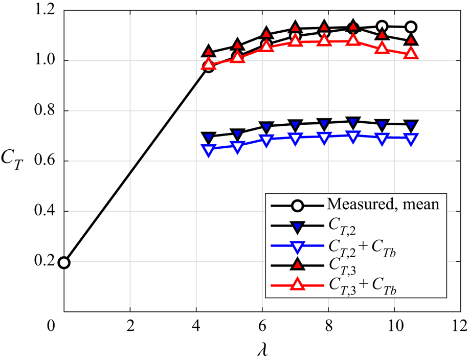
With  $u_{ze} > 1$ for all tip speed ratios considered, the correction given by (6.4) is negative, decreasing the thrust estimate when applied, and thus blockage cannot explain the discrepancy between
 $C_{T,2}$ and the measured thrust. Moreover, the correction is small, amounting to approximately
 $5\,\%$ of the measured thrust curve for all tip speed ratios. The values of
 $C_{T,2}$ and
 $C_{T,2} + C_{T,b}$ are plotted alongside the mean measured thrust curve in figure 12.
Thrust curves showing the estimated effect of blockage on the impulse-based thrust calculation. The correction  $C_{T,b}$ comes from (6.4). Blockage does not account for the discrepancy between
 $C_{T,2}$ and the mean measured thrust curve.

The parameters  $C_{T,3}$ and
 $C_{T,3} + C_{T,b}$ are also plotted in figure 12. The negative correction
 $C_{T,b}$ tends to improve the agreement between the calculated and measured thrust at low tip speed ratios, but it exacerbates the disagreement at the highest tip speed ratio, resulting in
 $C_{T,3} + C_{T,b}$ being
 $10\,\%$ below the measured thrust coefficient at the highest tip speed ratio. In any case, this correction does not invalidate the conclusion that the zero-strain-rate hypothesis is the most promising of those presented.
6.3. A physical explanation for the inaccuracy of $C_{T,1}$

As tip speed ratio is increased from the power optimum to the runaway condition, thrust is expected to increase as power decreases. Classical treatments cannot capture this trend, because they inherently assume that all generated thrust does useful work. In the 1-D limit, where  $a$ is constant over the swept disk of the rotor, it is assumed that
 $C_P = (1-a) C_T$. Noting the qualitative similarity between the plots of
 $C_P$ and
 $C_{T,1}$ vs
 $\lambda$ – figures 8 and 9, respectively – one might conclude that a similar assumption is inherent to the derivation of
 $C_{T,1}$.
The explicit assumption leading to  $C_{T,1}$ is the alignment of mean vortex lines and streamlines in the rotating frame of reference. This led, in Limacher & Wood (Reference Limacher and Wood2021), to the recovery of the Kutta–Joukowsky (KJ) equation for blade-element thrust. That equation is itself based on an idealized flow configuration – it is typically derived for an isolated airfoil in an unbounded flow – so it is not surprising that the assumptions leading to it preclude the possibility of parasitic drag.
Although the error-amplification explanation offered in § 5.4 is plausible, the correlation between  $C_{T,1}(\lambda )$ and
 $C_P(\lambda )$ suggests that
 $C_{T,1}$ fails for a physical reason. Since the high-thrust regime is usually associated with a turbulent wake state, we may conclude that turbulent diffusion creates a misalignment of mean vortex lines and streamlines, invalidating both
 $C_{T,1}$ and the KJ equation that can be derived from it.
6.4. Application to BEM theory
Although  $C_{T,3}$ is able to predict thrust better than the classical expression from momentum theory, it requires further simplification for implementation in BEM models. The full equation for
 $C_{T,3}$, given in (3.5), requires knowledge of
 $\omega _z(r,\theta,0)$ and
 $u_r(r,\theta,0)$ on a plane extending beyond the rotor radius, whereas BEM models depend only on
 $u_\theta$ and
 $a$ on
 $r \in [0,1]$.
First, we can invoke the assumption that  $a =0$ for
 $r>1$, allowing us to start from (3.6). Second, our results suggest that we can likely neglect the
 $\omega _z$-term for most operating conditions, although further investigation of its significance at lower tip speed ratios (
 $\lambda <4$) is warranted.
As for the contribution of  $u_r^{2}$, it may be related to that of
 $a^{2}$. In Limacher & Wood (Reference Limacher and Wood2021), it was shown that, for a circumferentially uniform flow through an actuator disk
 \begin{equation} \int_{S_D} \{u_r^{2} - a^{2}\}{\rm d}S = 0. \end{equation}
This does not strictly hold for a rotor, and it was not satisfied in our results, but the  $u_r^{2}$-contribution was small across the tip speed ratios considered, and an approximate relationship to the
 $a^{2}$-contribution could provide adequate accuracy for the purposes of BEM.
In sum, the assumption of zero strain rates in trailing vortex cores, coupled with the additional simplifications just noted, yield the following practical thrust equation:
 \begin{equation} C_T = \int_{S_D} \{u_\theta^{2} + ka^{2} + 4a(1-a) \} {\rm d}S, \end{equation}
where  $k$ is a factor to be determined empirically or theoretically.
Since BEM models do predict peak power with acceptable accuracy, it is sensible to retain the classical expression of  $C_P = 4a(1-a)^{2}$. In so doing, we avoid the assumption that all generated thrust does useful work, with the squared-velocity terms in (6.7) serving as estimates of the parasitic component of the rotor drag.
7. Conclusions
The present work contributes to a reconsideration of wind turbine theory through the lens of vortical impulse theory. Contrary to momentum theory, impulse theory expresses linear momentum conservation in terms of velocity and vorticity, rather than velocity and pressure, and this removal of pressure facilitates direct treatment of the near wake. The high-thrust regime that remains theoretically unexplained by momentum theory – occurring between the power-optimal tip speed ratio and the runaway speed – is a specific focus of this work.
Starting from a general impulse-based thrust expression for steadily rotating turbines in an unbounded, incompressible flow, simplified expressions were derived by invoking three distinct physical assumptions, which are: (i) the alignment of mean streamlines and vortex lines in the rotor-fixed frame of reference; (ii) the insignificance of  $\partial u_r/\partial z$ in the immediate vicinity of the rotor; and (iii) zero-strain rates in the cores of the trailing vortices.
From a theoretical perspective, the last proposition is the most intriguing, as its corresponding thrust expression includes the familiar  $4a(1-a)$ integrand from classical turbine theory, plus novel squared-velocity terms that permit a monotonic increase in thrust across all induction factors,
 $a \in [0,1]$.
Experimentally, the thrust expressions resulting from the three physical propositions were tested using stereo-PIV data on a stream-normal plane just behind a rotor, operating in a water channel. The acquired velocity fields were used as inputs to discretized versions of the various impulse-derived thrust expressions, and the zero-strain-rate hypothesis gave the best agreement with the directly measured thrust, yielding a worst-case error of  $5.7\,\%$ relative to the measured thrust, or
 $10\,\%$ after approximate blockage correction. We thus have the satisfying result that the best-performing expression for experimental thrust estimation is simultaneously the most theoretically appealing. These results offer motivation for future experimental (or numerical) studies to investigate strain rates in the near wake of rotors.
Possible sources of error were investigated to estimate their plausible significance, all of which were deemed minor. Increased spatial resolution was shown to have minimal effect on the force estimates, and insufficient resolution could not explain the discrepancies between measured and calculated forces using the first two propositions. Tunnel blockage was also considered, but its estimated significance, as determined from velocity data at the edge of the investigated domain, is only about  $5\,\%$ of the measured thrust. Nonlinear contributions to the mean thrust due to rotor-speed variability have been argued to be small (
 ${<}5\,\%$) by means of an order-of-magnitude analysis. However, one cannot dismiss altogether the possibility of nonlinear contributions due to turbulence, and future work is recommended to directly investigate their significance.
The failure of the thrust expressions derived from the first two physical propositions was attributed to the invalidity of the propositions themselves. The first proposition, regarding streamline and vortex line alignment, appears to imply that most of the generated thrust does useful work. This assumption, which is also inherent to classical momentum theory, is clearly invalid in the high-thrust regime considered herein. The second and third propositions are mutually exclusive, and the experimental results suggest that proposition (ii) should be discarded in favour of proposition (iii).
The thrust expression arising from proposition (iii) cannot be directly implemented in BEM codes, because it depends on the radial velocity and axial vorticity. A brief discussion is offered as to how this general thrust expression might be simplified, recovering a useful thrust expression that, like existing BEM models, depends only on circumferential and axial velocities in the vicinity of the rotor.
Funding
The authors would like to acknowledge the financial support of the following grants: NSF CBET 1652583, and ONR Grant N00014-17-1-2309 (Program Manager P. Chang). The lead author also acknowledges receipt of an NSERC Post-Doctoral Fellowship award.
Declaration of interests
The authors report no conflicts of interest.