The bryozoan genus Cauloramphus Norman, 1903, is distributed worldwide with at least 25 living species in the genus (Dick et al., Reference Dick, Lidgard, Gordon and Mawatari2009, Reference Dick, Mawatari, Sanner and Grischenko2011). In some regions of the world, such as the North Pacific, it is one of the most speciose anascan genera (Grischenko et al., Reference Grischenko, Dick and Mawatari2007). However, currently only one species of Cauloramphus has been recorded from around the United Kingdom. Cauloramphus spinifer (Johnston, 1832) has a circumpolar Arctic–boreal distribution (Dick & Mawatari, Reference Dick, Mawatari, Mawatari and Okada2004) and has been commonly recorded on rocky shores in the British Isles, from the mid-shore to the shallow sublittoral, encrusting substrata such as stones, shells and kelp holdfasts (Hayward & Ryland, Reference Hayward and Ryland1998). This description of the distribution has not changed since Hincks’ (Reference Hincks1880) work was published at the height of the Victorian period of marine invertebrate exploration. Localities listed by Hincks for C. spinifer (as Membranipora spinifera) are all ‘between tide marks’, despite the fact that there is a mention that Alder found examples of this species offshore around the Northumberland coast.

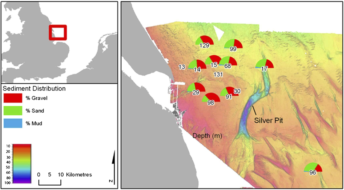
During April and May 2009 a Regional Environmental Characterization (REC) survey of the Humber area of the North Sea was carried out aboard the MV ‘Sea Profiler’. One hundred and forty seabed samples were acquired using a mini Hamon grab and preserved in 4% formaldehyde solution in seawater. The samples were later transferred to 70% industrial methylated spirits for processing. Thirteen of the samples, all of which were located further than 5.5 km offshore, contained Cauloramphus spinifer. Their depths ranged from 14.9 m at Station 98 to a maximum of 53.1 m at Station 17 located on the edge of Silver Pit, a palaeo-tunnel valley situated within the survey area (Figure 1).

Fig. 1.

Map of the Humber area of the North Sea indicating the locations and depths of samples containing Cauloramphus spinifer with associated sediment composition charts (Stations 13, 30 and 131 do not have sediment data).

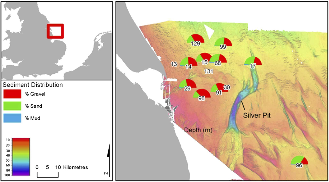
The sediment type for all the stations with Cauloramphus spinifer present was similar, comprising mixtures of gravel and sand (Figure 1). All stations with particle size data available were classified as sandy-gravel, except Stations 91 and 98 which were gravelly muddy-sand and Station 129 which was muddy sandy-gravel. This reflects the mode of life of Bryozoa. As sedentary encrusting fauna they require substrate such as stones, shells or shell fragments to attach to and any excess of fine particles will hinder the colony's ability to filter feed.

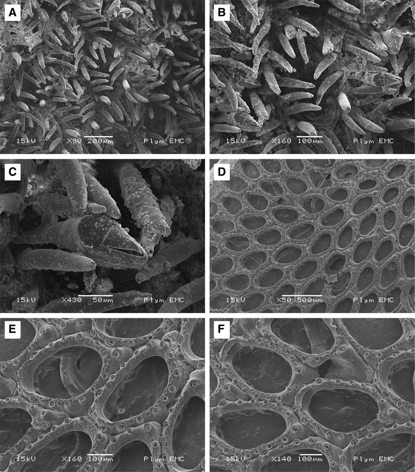
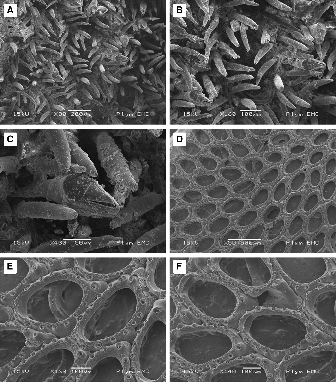
The specimens were identified using the key developed by Hayward & Ryland (Reference Hayward and Ryland1998), and further investigation showed that the specimens from the REC were not compatible with published descriptions of any other Cauloramphus species (Dick et al., Reference Dick, Grischenko and Mawatari2005, Reference Dick, Mawatari, Sanner and Grischenko2011; Grischenko et al., Reference Grischenko, Dick and Mawatari2007). The opesia is oval and takes up most of the frontal surface. Specimens have 12–16 spines, which overarch the opesia. Stalked avicularia occur singularly, lateral to the orifice, between spines. The avicularian peduncle is approximately the same length as the spines; the rostrum is situated at the top edge of the peduncle pointing inwards and the mandible points upwards. Ooecia were present, visible as a simple cap-like structure at the distal end of the zooid as discussed by Ostrovsky et al. (Reference Ostrovsky, Dick and Mawatari2007). These characteristics are consistent with the description of C. spinifer published by Hayward & Ryland (Reference Hayward and Ryland1998) and De Blauwe (Reference De Blauwe2009) for UK waters but the spines are more numerous than on specimens described in the Kurile Islands (Mawatari, Reference Mawatari1956) and Alaska (Grischenko et al., Reference Grischenko, Dick and Mawatari2007).

Dried specimens were prepared for scanning electron microscope (SEM) examination by coating in gold. Further specimens were bleached for one hour in sodium hypochlorite 1% ww, then rinsed with water to remove the spines before air drying and coating. Scanning electron micrographs (Figure 2) were taken using a JEOL 5600LV SEM which show details of the spines, avicularia and ooecia.

Fig. 2.

Cauloramphus spinifer. (A) Group of zooids, unbleached; (B) close-up of zooid showing details of spines and avicularia, unbleached; (C) detail of stalked aviculairum; (D) Colony, bleached; (E) close-up of bleached zooids showing connecting pores; (F) close-up of zooids showing ooecia.

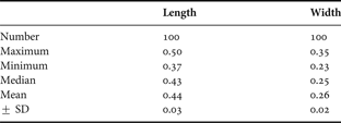
Measurements of zooids were taken at ×50 magnification using a Zeiss Stemi 2000 stereoscopic microscope fitted with an ocular micrometer. Twenty zooids per colony from five separate colonies were measured. Length-ranges were 0.37–0.50 mm and widths were 0.23–0.35 mm (Table 1), and between the colonies lengths and widths showed little variation. These measurements agree very closely with those recorded by Hayward & Ryland (Reference Hayward and Ryland1998) from British waters, 0.40–0.52 mm length and 0.26–0.3 mm width. However, there seems to be a geographical variation with the measurements from the UK being smaller than the sizes recorded by Grischenko et al. (Reference Grischenko, Dick and Mawatari2007) from Hokkaido, Japan, 0.47–0.60 mm length and 0.30–0.40 mm width and Shunatova & Ostrovsky (Reference Shunatova and Ostrovsky2001) from the White Sea, 0.45–0.65 mm length and 0.30–0.35 mm width. The larger size of the zooids from the White Sea can be explained due to the lower sea temperatures occurring in this area. Zooid size has been shown to conform to Bergmann's rule where body size is inversely linked with sea temperature. Many authors have shown that the ultimate size of zooids in cheilostome bryozoans is controlled to a significant extent by the temperature at which the zooid was budded. This has been recorded both in the natural environment (Okamura & Bishop, Reference Okamura and Bishop1988; O'Dea & Okamura, Reference O'Dea and Okamura2000; O'Dea, Reference O'Dea2003; Lombardi et al., Reference Lombardi, Cocito, Occhipinti-Ambrogi and Hiscock2006) and in experimental laboratory conditions (O'Dea & Jackson, Reference O'Dea and Jackson2002; Amui-Vedel et al., Reference Amui-Vedel, Hayward and Porter2007). The difference in zooid size between the REC samples and the zooids from Japan is harder to explain as the sea temperatures in Hokkaido range between 21.1°C and −1.4°C (Grischenko et al., Reference Grischenko, Dick and Mawatari2007), which is similar to the temperature range in the North Sea. The lowest temperature recorded in the North Sea near the REC site is 1.5°C in 1986, however, since the start of this century the lowest recorded temperature has not fallen below 4.5°C (www.cefas.defra.gov.uk). Although maximum and minimum temperatures do not allow an accurate assessment of the temperature regime under which the zooids were budded, the lower minimum temperatures in Hokkaido may mean that the bryozoans there generally experience lower mean annual temperatures which would explain the size difference. However, as pointed out in Lombardi et al. (Reference Lombardi, Cocito, Occhipinti-Ambrogi and Hiscock2006) the possibility that the difference is due to the presence of a cryptic species should be considered.

Table 1.

Cauloramphus spinifer zooid length and width measurements in mm. Measurements taken from five separate colonies, 20 zooids per colony.

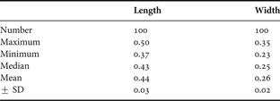
SD, standard deviation.

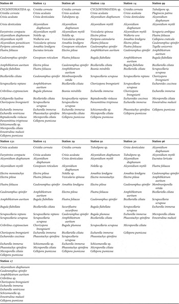
There were many other bryozoan species present in the samples alongside Cauloramphus spinifer (Table 2). In all 47 species of ctenostome, cheilostome and cyclostomes, bryozoans were present in the thirteen samples. The sample with the most abundant bryozoan diversity was Station 68 with 26 species present. Station 17, the deepest of the stations on the edge of Silver Pit, had relatively poor bryozoan abundance, only ten species. The ctenostome bryozoan Alcyonidium diaphanum (Hudson, 1778) and the cheilostome bryozoan Escharella immersa (Fleming, 1828) were associated with Cauloramphus spinifer in every sample. Amphiblestrum auritum (Hincks, 1877) and Cellepora pumicosa (Pallas, 1766), both cheilostome Bryozoa, were present in all but one of the samples considered. Also worthy of note is Cribrilina cryptooecium Norman, 1903, a cheilostome bryozoan listed as occurring commonly in association with Cauloramphus spinifer (Hayward & Ryland, Reference Hayward and Ryland1998). It was present in two stations, Station 68 and Station 131, which were 28.1 m and 22.5 m respectively. This indicates that associations known to occur in shallower water still occur at increased depth.

Table 2.

Species lists of Bryozoa found in samples containing Cauloramphus spinifer. Columns arranged in order of abundance of Bryozoa per site.

It has previously been considered that C. spinifer was not found below the depth of the kelp bed (Hayward & Ryland, Reference Hayward and Ryland1998). Little & Kitching (Reference Little and Kitching2001) stated the normal depth limit for kelp beds in western Europe is 17–20 m below chart datum where light becomes a growth limiting factor. However, off south-west Ireland the lower limit of kelp has been reported as approaching 30 m (Edwards, Reference Edwards1980). This is possible in clear, less turbid water where light penetrates further. Seven out of the thirteen samples containing C. spinifer were below 20 m depth, with a maximum recorded depth of 53.1 m, therefore constituting new bathymetric records for this species.

Although depth is often used as a defining factor in the distribution of marine species it is not the only, or necessarily most important, factor that influences distributions, and there is no reason why depth per se should control bryozoan distributions (Taylor et al., Reference Taylor, Gordon and Batson2004). Distributions of bryozoans are controlled by a group of interrelated factors such as nutrients, temperature, water chemistry, substrate and currents (Hageman et al., Reference Hageman, Bone, McGowran and James1995). These environmental factors vary with depth and so these depth-correlated factors as a set of environmental conditions will play roles in defining the boundaries of a species distribution. We could, therefore, expect to find Cauloramphus spinifer at depth wherever the factors combine to produce a favourable set of environmental conditions.

The finding of these specimens significantly extends the known depth-range of this species. As the REC survey was carried out in order to provide wider geographical information to enhance the results of localized environmental impact assessments, it is possible that this depth-range has not been recorded before due to lack of sampling. Potentially, with further sampling effort more examples of Cauloramphus spinifer will be found at depths below the kelp bed.