1 Introduction
Fluid flow through strongly deformable media is an important feature of many natural systems. One prominent mechanism is flow through pipe-like conduits embedded in a viscously deformable solid matrix. The two primary geophysical applications for this class of model are found in magma dynamics and subglacial hydrology. Solitary waves were recognized as solutions to the equations governing magma dynamics where the matrix is mantle rock and the fluid is silicate melt (Scott & Stevenson Reference Scott and Stevenson1984; Olson & Christensen Reference Olson and Christensen1986; Helfrich & Whitehead Reference Helfrich and Whitehead1990). These waves are localized ‘bumps’ of excess fluid above a background state that travel with constant speed and permanent form. They arise when viscous closure of the conduit walls at the upstream end of the wave is balanced by opening at the downstream end.
Solitary waves in deformable conduits have been produced with laboratory experiments where a variety of fluids have been used to model the two phases (Olson & Christensen Reference Olson and Christensen1986; Scott, Stevenson & Whitehead Reference Scott, Stevenson and Whitehead1986; Lowman, Hoefer & El Reference Lowman, Hoefer and El2014; Meyer, Hewitt & Neufeld Reference Meyer, Hewitt and Neufeld2017). Most analytical work has since focused on a closely related model of fluid flow through deformable permeable media, although the one-dimensional model is identical to the conduit model in the case of a linear solid rheology and laminar fluid flow for a certain parameter range. In the permeable media model, questions concerning the formation of dispersive wave trains and nonlinear stability of the wave forms have been addressed (Barcilon & Richter Reference Barcilon and Richter1986; Barcilon & Lovera Reference Barcilon and Lovera1989; Spiegelman Reference Spiegelman1993a,Reference Spiegelmanb; Simpson & Weinstein Reference Simpson and Weinstein2008; Simpson, Weinstein & Rosenau Reference Simpson, Weinstein and Rosenau2008; Lowman & Hoefer Reference Lowman and Hoefer2013b).
While solitary waves have been a prominent research topic in magma dynamics, the discussion in subglacial hydrology has been limited despite the similarity between the governing equations. The primary difference between the mechanical components of these systems is that magma dynamics typically assumes laminar flow through a Newtonian matrix, whereas subglacial hydrology models assume turbulent flow through a power-law material. We show that both models can be included in a single description.
In subglacial hydrology, the idealized conduit is a circular or semi-circular channel through which water flows at or near the base of a glacier. The classical theory of these channels by Röthlisberger (Reference Röthlisberger1972) and Nye (Reference Nye1976) has since been extended to include other types of drainage elements such as linked cavities that open due to sliding of the overlying ice and macroporous water sheets (Creyts & Schoof Reference Creyts and Schoof2009; Hewitt Reference Hewitt2011; Hewitt, Schoof & Werder Reference Hewitt, Schoof and Werder2012; Schoof, Hewitt & Werder Reference Schoof, Hewitt and Werder2012). However, the only discussion of solitary waves in this context is by Meyer et al. (Reference Meyer, Hewitt and Neufeld2017).
Other wave-like phenomena on the glacier surface and in subglacial drainage systems have been studied (Fowler Reference Fowler1982; Hewitt & Fowler Reference Hewitt and Fowler2008; Schoof et al. Reference Schoof, Hewitt and Werder2012). Since glacier acceleration due to basal sliding is strongly influenced by water pressure variations at the base, certain classes of surface waves likely correspond to waves in the subglacial drainage system. In this vein, a solitary mass-transport wave on the Greenland Ice Sheet was recently observed using geodetic measurements by Adhikari, Ivins & Larour (Reference Adhikari, Ivins and Larour2017). The hypothesized mechanism of wave formation included enhanced subglacial activity due to influx of meltwater, although no precise connection was drawn.
The discussion of waves has not been limited to Earth’s ice–water system. Porosity waves were proposed to be an efficient mechanism for water transport through Europa’s icy crust to its subsurface ocean by Kalousová et al. (Reference Kalousová, Souček, Tobie, Choblet and Čadek2014) who used a permeable media model similar to the one discussed above. Of course, this idea could be extended to the icy moons Ganymede and Enceladus, which also possess subsurface water bodies (Spohn & Schubert Reference Spohn and Schubert2003). Given that some of these bodies potentially support life, understanding the dynamics of these large scale ice–water systems has become increasingly important (Spencer & Nimmo Reference Spencer and Nimmo2013).
In this paper, we present a unified treatment of fluid flow through viscously deformable conduits (§§ 2–3), demonstrate the formation of solitary wave trains with numerical experiments (§ 4), prove the existence of solitary wave solutions for a wide range of parameters (§ 5.1) and explore rheology-dependent flattening of the waves (§ 5.2). While phase change is important in all of the above applications and is often included in computational studies, we only explore it here briefly in the context of subglacial hydrology since the solutions do not travel with constant speed and permanent form (§ 6).
2 Generalized model
We consider a two phase system where the fluid flows through a pipe-like conduit embedded in a viscously deformable solid matrix. For simplicity, we will assume a radially symmetric conduit of circular cross-section with an infinitely thick outer wall. This assumption is reasonable in most geophysical applications where the radius of the conduit is small compared to the length scale of the solid matrix. As stated above, we will neglect mass transfer between the phases. This assumption is often reasonable in magma dynamics when the melt is in thermal and chemical equilibrium with the wall rock. However, in glaciology it is not widely applicable because phase change drives many important processes such as glacial outburst floods and basal sliding (Fowler Reference Fowler1999; Hewitt Reference Hewitt2013). We revisit this assumption and explore the existence of solitary wave-like phenomena in a subglacial channel model with discharge-dependent melting after the forthcoming analysis (§ 6).
We let  $x$ be the along-conduit coordinate,
 $S$ the cross-sectional area of the conduit,
 $Q$ the volumetric fluid flux,
 $p_{s}$ the solid pressure and
 $p_{f}$ the fluid pressure. Instead of working with these two pressures separately, we define an effective pressure as
 $N=p_{s}-p_{f}$. We assume that the solid is incompressible and deforms according to a power-law rheology of the form
 $$\begin{eqnarray}\dot{\unicode[STIX]{x1D716}}=\hat{A}\unicode[STIX]{x1D70F}_{e}^{n-1}\unicode[STIX]{x1D70F},\end{eqnarray}$$
where  $\unicode[STIX]{x1D70F}_{e}^{2}={\textstyle \frac{1}{2}}\text{tr}(\unicode[STIX]{x1D70F}^{2})$ is the second invariant of the deviatoric stress tensor
 $\unicode[STIX]{x1D70F}$,
 $\dot{\unicode[STIX]{x1D716}}$ is the strain rate tensor, the constant
 $\hat{A}>0$ depends on material properties and the stress exponent
 $n\geqslant 1$ is taken to be constant. Equation (2.1) with
 $n=3$ is known as Glen’s law in glaciology (Glen Reference Glen1958; Cuffey & Paterson Reference Cuffey and Paterson2010). Fluid flow is modelled by either a laminar or turbulent parameterization defined by (2.4), which is general enough to encompass both models. The primary assumptions in deriving (2.2)–(2.4) are that (I) surface tension between the phases is negligible and (II) the slope of the solid–fluid interface is small (Nye Reference Nye1976; Lowman & Hoefer Reference Lowman and Hoefer2013a; Evatt Reference Evatt2015). Conservation of mass and momentum for the solid and fluid phases is then satisfied through the following set of equations:
 $$\begin{eqnarray}\displaystyle & \displaystyle \frac{\unicode[STIX]{x2202}S}{\unicode[STIX]{x2202}t}=-\frac{\unicode[STIX]{x2202}Q}{\unicode[STIX]{x2202}x}, & \displaystyle\end{eqnarray}$$
 $$\begin{eqnarray}\displaystyle & \displaystyle \frac{\unicode[STIX]{x2202}Q}{\unicode[STIX]{x2202}x}=KS|N|^{n}\text{sgn}(N), & \displaystyle\end{eqnarray}$$
 $$\begin{eqnarray}\displaystyle & \displaystyle Q=\unicode[STIX]{x1D6FE}S^{\unicode[STIX]{x1D6FC}}\left|\unicode[STIX]{x1D713}_{0}+\frac{\unicode[STIX]{x2202}N}{\unicode[STIX]{x2202}x}\right|^{\unicode[STIX]{x1D6FD}}\text{sgn}\left(\unicode[STIX]{x1D713}_{0}+\frac{\unicode[STIX]{x2202}N}{\unicode[STIX]{x2202}x}\right). & \displaystyle\end{eqnarray}$$
Equation (2.2) is a continuity equation, while (2.3) and (2.4) ensure conservation of momentum for the solid and fluid, respectively. The term  $S|N|^{n}\text{sgn}(N)$ in (2.3) represents viscous closure of the conduit walls and is derived directly from the Stokes equations by Evatt (Reference Evatt2015), although the original derivation is due to Nye (Reference Nye1953). Equations (2.2)–(2.4) are a generalized version of those derived by Nye (Reference Nye1976) with melting neglected.
All derivations of the viscous closure rate assume that the solid flows only in the radial direction and is azimuthally symmetric, which has recently been called into question (Dallaston & Hewitt Reference Dallaston and Hewitt2014; Meyer et al. Reference Meyer, Fernandes, Creyts and Rice2016). For our model, the main effect would be to perturb the conduit cross-section away from a circular shape. The evolution of circular and non-circular conduits has been explored by Dallaston & Hewitt (Reference Dallaston and Hewitt2014) in the context of subglacial hydrology. Since this is unlikely to have an effect of the formation of solitary waves, we do not pursue this further. Above,  $K=2\hat{A}n^{-n}$ is the ice flow-law coefficient,
 $\unicode[STIX]{x1D713}_{0}>0$ is the hydraulic gradient and
 $(\unicode[STIX]{x1D6FC},\unicode[STIX]{x1D6FD},\unicode[STIX]{x1D6FE})$ are positive constants in the fluid flow parameterization. Below we will assume that
 $\unicode[STIX]{x1D713}_{0}$ is constant for simplicity, although spatially varying hydraulic gradients are important in many applications (Fowler Reference Fowler1999).
3 Scaling
In order to scale the system (2.2)–(2.4), we introduce the following non-dimensional variables and characteristic units, denoted with primes and tildes, respectively.
 $$\begin{eqnarray}x=\tilde{x}x^{\prime },\quad t=\tilde{t}t^{\prime },\quad S=\tilde{S}S^{\prime },\quad Q=\tilde{Q}Q^{\prime },\quad N={\tilde{N}}N^{\prime }.\end{eqnarray}$$
The characteristic units are defined up to an arbitrary choice of  $\tilde{S}$ as follows:
 $$\begin{eqnarray}\left.\begin{array}{@{}c@{}}\tilde{Q}=\unicode[STIX]{x1D6FE}\tilde{S}^{\unicode[STIX]{x1D6FC}}\unicode[STIX]{x1D713}_{0}^{\unicode[STIX]{x1D6FD}},\\ \tilde{x}=[\tilde{Q}(K\tilde{S}\unicode[STIX]{x1D713}_{0}^{n})^{-1}]^{1/n+1},\\ {\tilde{N}}=\tilde{x}\unicode[STIX]{x1D713}_{0},\\ \tilde{t}=\tilde{S}\tilde{x}\tilde{Q}^{-1}.\end{array}\right\}\end{eqnarray}$$
With the definitions in (3.2), equations (2.2)–(2.4) simplify to the following non-dimensional form after dropping primes:
 $$\begin{eqnarray}\displaystyle & \displaystyle \frac{\unicode[STIX]{x2202}S}{\unicode[STIX]{x2202}t}=-\frac{\unicode[STIX]{x2202}Q}{\unicode[STIX]{x2202}x}, & \displaystyle\end{eqnarray}$$
 $$\begin{eqnarray}\displaystyle & \displaystyle \frac{\unicode[STIX]{x2202}Q}{\unicode[STIX]{x2202}x}=S|N|^{n}\text{sgn}(N), & \displaystyle\end{eqnarray}$$
 $$\begin{eqnarray}\displaystyle & \displaystyle Q=S^{\unicode[STIX]{x1D6FC}}\left|1+\frac{\unicode[STIX]{x2202}N}{\unicode[STIX]{x2202}x}\right|^{\unicode[STIX]{x1D6FD}}\text{sgn}\left(1+\frac{\unicode[STIX]{x2202}N}{\unicode[STIX]{x2202}x}\right). & \displaystyle\end{eqnarray}$$
We assume the following throughout:
 $$\begin{eqnarray}n\geqslant 1,\quad \unicode[STIX]{x1D6FC}>1,\quad \unicode[STIX]{x1D6FD}>0.\end{eqnarray}$$
Equation (3.4) may be written as  $N=S^{-(1/n)}|\unicode[STIX]{x2202}Q/\unicode[STIX]{x2202}x|^{1/n}\text{sgn}(\unicode[STIX]{x2202}Q/\unicode[STIX]{x2202}x)$. Taking the
 $x$-derivative of (3.5), and using this identity along with (3.3), we obtain
 $$\begin{eqnarray}\frac{\unicode[STIX]{x2202}S}{\unicode[STIX]{x2202}t}+\frac{\unicode[STIX]{x2202}}{\unicode[STIX]{x2202}x}\left\{S^{\unicode[STIX]{x1D6FC}}\left[1-\frac{\unicode[STIX]{x2202}}{\unicode[STIX]{x2202}x}\left(\text{sgn}\left(\frac{\unicode[STIX]{x2202}S}{\unicode[STIX]{x2202}t}\right)\left|S^{-1}\frac{\unicode[STIX]{x2202}S}{\unicode[STIX]{x2202}t}\right|^{1/n}\right)\right]^{\unicode[STIX]{x1D6FD}}\right\}=0,\end{eqnarray}$$
where we have temporarily assumed  $Q\geqslant 0$ for simplicity. In the case
 $(\unicode[STIX]{x1D6FC},\unicode[STIX]{x1D6FD},n)=(2,1,1)$, this is the classical conduit equation of magma dynamics where the fluid flow is laminar and the solid rheology is linear (Olson & Christensen Reference Olson and Christensen1986; Lowman & Hoefer Reference Lowman and Hoefer2013a; Lowman et al. Reference Lowman, Hoefer and El2014). The following nonlinear dispersive wave equation is closely related to (3.7) and was studied by Simpson et al. (Reference Simpson, Weinstein and Rosenau2008).
 $$\begin{eqnarray}\frac{\unicode[STIX]{x2202}\unicode[STIX]{x1D719}}{\unicode[STIX]{x2202}t}+\frac{\unicode[STIX]{x2202}}{\unicode[STIX]{x2202}x}\left\{\unicode[STIX]{x1D719}^{\unicode[STIX]{x1D6FC}}\left[1-\frac{\unicode[STIX]{x2202}}{\unicode[STIX]{x2202}x}\left(\unicode[STIX]{x1D719}^{-m}\frac{\unicode[STIX]{x2202}\unicode[STIX]{x1D719}}{\unicode[STIX]{x2202}t}\right)\right]\right\}=0.\end{eqnarray}$$
In (3.8),  $\unicode[STIX]{x1D719}$ is the porosity of the solid matrix, and
 $m$ is a rheological constant. In the special case
 $m=1$, equation (3.8) is also identical to (3.7) with the choice
 $(\unicode[STIX]{x1D6FC},\unicode[STIX]{x1D6FD},n)=(2,1,1)$. However, equations (3.7) and (3.8) are distinct if any nonlinear rheology or turbulence parameterization is included.
The parameter choices  $(\unicode[STIX]{x1D6FD},n)=({\textstyle \frac{1}{2}},3)$ are associated with the subglacial channel equations in the absence of melting (Nye Reference Nye1976). The values
 $\unicode[STIX]{x1D6FC}={\textstyle \frac{5}{4}}$ and
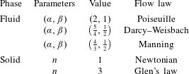
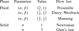
 $\unicode[STIX]{x1D6FC}={\textstyle \frac{4}{3}}$ are often chosen in this case, corresponding to the Darcy–Weisbach and Manning parameterizations of turbulent water flow, respectively (Clarke Reference Clarke2003). Since the mechanical component of nearly all subglacial hydrology models is closely related to (3.3)–(3.5), the analysis presented herein is widely applicable. As we will show, solitary wave solutions to (3.7) exist in both the magmatic and glacial parameter regimes. We explore the effect of these different parameter choices in the following section. We provide a summary of these parameters and related flow laws in table 1.
Summary of the solid and fluid flow laws discussed in the text.
4 Numerical results
In order to construct a reference solution for comparison with the full nonlinear equations, we consider the simplification  $\unicode[STIX]{x2202}N/\unicode[STIX]{x2202}x\approx 0$. Using the resulting identity
 $Q=S^{\unicode[STIX]{x1D6FC}}$ from (3.5), this reduces (3.3) to a kinematic wave equation for
 $S$.
 $$\begin{eqnarray}\frac{\unicode[STIX]{x2202}S}{\unicode[STIX]{x2202}t}+\unicode[STIX]{x1D6FC}S^{\unicode[STIX]{x1D6FC}-1}\frac{\unicode[STIX]{x2202}S}{\unicode[STIX]{x2202}x}=0.\end{eqnarray}$$
Equation (4.1) shows that the system is purely hyperbolic in the absence of pressure variations associated with viscous deformation of the conduit. We make the parameterization  $S=S(x(t(\unicode[STIX]{x1D70F})),t(\unicode[STIX]{x1D70F}))$, which upon substitution in (4.1) leads to the equivalent system of ordinary differential equations
 $$\begin{eqnarray}\displaystyle & \displaystyle \frac{\text{d}S}{\text{d}\unicode[STIX]{x1D70F}}=0, & \displaystyle\end{eqnarray}$$
 $$\begin{eqnarray}\displaystyle & \displaystyle \frac{\text{d}x}{\text{d}\unicode[STIX]{x1D70F}}=\unicode[STIX]{x1D6FC}S^{\unicode[STIX]{x1D6FC}-1}, & \displaystyle\end{eqnarray}$$
 $$\begin{eqnarray}\displaystyle & \displaystyle \frac{\text{d}t}{\text{d}\unicode[STIX]{x1D70F}}=1,\quad t(0)=0. & \displaystyle\end{eqnarray}$$
Following previous studies, we set up a Riemann problem to find an initial condition that develops into a step shock (Spiegelman Reference Spiegelman1993b; Lowman & Hoefer Reference Lowman and Hoefer2013b). We let  $\unicode[STIX]{x1D70F}_{s}$ be the time of shock formation with characteristics
 $x(\unicode[STIX]{x1D70F}_{s})=x_{s}$, where
 $x_{s}=x_{\ast }$ is the position of the shock. Then we have
 $$\begin{eqnarray}S(x_{s},\unicode[STIX]{x1D70F}_{s})=\left\{\begin{array}{@{}ll@{}}1\quad & x_{s}<x_{\ast },\\ S_{0}\quad & x_{s}\geqslant x_{\ast },\end{array}\right.\end{eqnarray}$$
where  $S_{0}<1$ denotes the magnitude of reduction in conduit size. With these initial data, the solutions of (4.2)–(4.3) are given by
 $$\begin{eqnarray}\displaystyle & S(x,\unicode[STIX]{x1D70F})=S(x_{s},\unicode[STIX]{x1D70F}_{s}), & \displaystyle\end{eqnarray}$$
 $$\begin{eqnarray}\displaystyle & x(\unicode[STIX]{x1D70F})=x_{s}+\unicode[STIX]{x1D6FC}S(x_{s},\unicode[STIX]{x1D70F}_{s})^{\unicode[STIX]{x1D6FC}-1}(\unicode[STIX]{x1D70F}-\unicode[STIX]{x1D70F}_{s}). & \displaystyle\end{eqnarray}$$
Substitution of (4.6)–(4.7) into (4.5) results in
 $$\begin{eqnarray}\left.\begin{array}{@{}c@{}}S(x(\unicode[STIX]{x1D70F}),\unicode[STIX]{x1D70F})=\left\{\begin{array}{@{}ll@{}}1\quad & x(\unicode[STIX]{x1D70F})<\unicode[STIX]{x1D707}_{1}(\unicode[STIX]{x1D70F})\\ S_{0}\quad & x(\unicode[STIX]{x1D70F})>\unicode[STIX]{x1D707}_{2}(\unicode[STIX]{x1D70F})\\ \left(\unicode[STIX]{x1D6FC}^{-1}{\displaystyle \frac{x(\unicode[STIX]{x1D70F})-x_{\ast }}{\unicode[STIX]{x1D70F}-\unicode[STIX]{x1D70F}_{s}}}\right)^{1/\unicode[STIX]{x1D6FC}-1}\quad & \unicode[STIX]{x1D707}_{1}(\unicode[STIX]{x1D70F})\leqslant x(\unicode[STIX]{x1D70F})\leqslant \unicode[STIX]{x1D707}_{2}(\unicode[STIX]{x1D70F})\quad (\text{for }\unicode[STIX]{x1D70F}<\unicode[STIX]{x1D70F}_{s})\end{array}\right.\\ \unicode[STIX]{x1D707}_{1}(\unicode[STIX]{x1D70F})=x_{\ast }+\unicode[STIX]{x1D6FC}(\unicode[STIX]{x1D70F}-\unicode[STIX]{x1D70F}_{s}),\quad \unicode[STIX]{x1D707}_{2}(\unicode[STIX]{x1D70F})=x_{\ast }+\unicode[STIX]{x1D6FC}S_{0}^{\unicode[STIX]{x1D6FC}-1}(\unicode[STIX]{x1D70F}-\unicode[STIX]{x1D70F}_{s}).\end{array}\right\}\end{eqnarray}$$
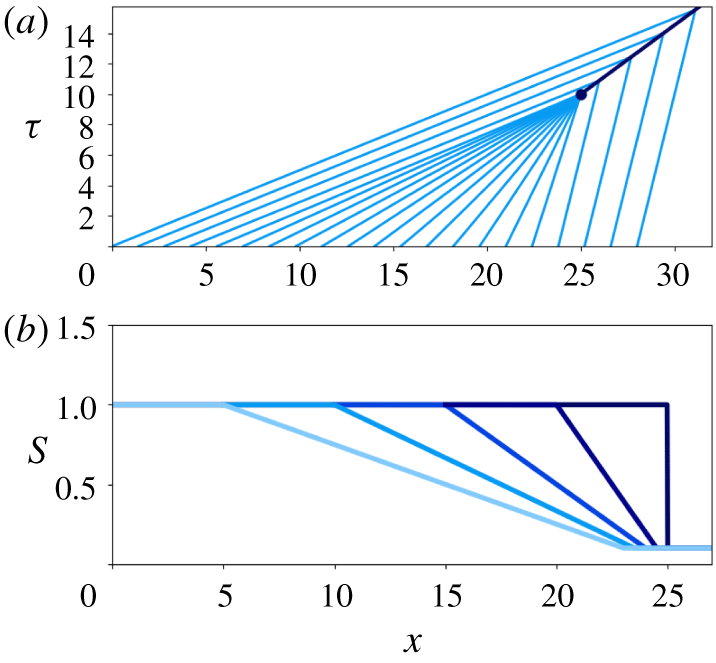
(a) Characteristics of (4.8) with  $(\unicode[STIX]{x1D6FC},\unicode[STIX]{x1D70F}_{s},x_{\ast },S_{0})=(2,10,25,0.05)$. The initial time and location of the shock is marked with a dark circle. (b) Evolution of the initial condition (light) into the step shock (dark) at
 $\unicode[STIX]{x1D70F}=\unicode[STIX]{x1D70F}_{s}$.
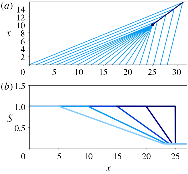
An example solution (4.8) to the approximation (4.1) and its characteristics are depicted in figure 1. We use a mixed finite element method to solve (3.3)–(3.5) with an initial condition  $S(x,0)$ given by (4.8) (appendix A). This initial condition is smoothed very slightly by convolution with a Gaussian in order to remove the sharp edges at
 $x=\unicode[STIX]{x1D707}_{\ell }$ in (4.8). The corresponding initial conditions are
 $Q(x,0)=S(x,0)^{\unicode[STIX]{x1D6FC}}$ and
 $N(x,0)$ is obtained from (3.4). We enforce the Dirichlet boundary condition
 $(S_{D},N_{D},Q_{D})=(1,0,1)$ at
 $x=0$ to be consistent with the approximate solution (4.8). Details on the weak formulation, time integration and implementation are provided in appendix A.
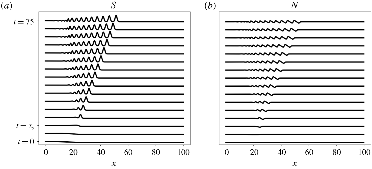
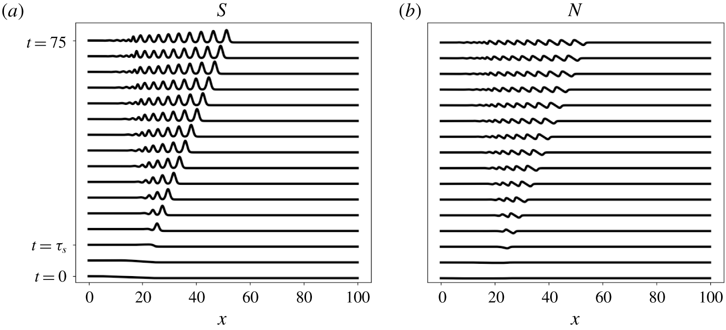
Numerical solution of the full nonlinear equations for  $x\in [0,100]$,
 $t\in [0,75]$, with the parameter choice
 $(\unicode[STIX]{x1D6FC},\unicode[STIX]{x1D6FD},n)=(2,1,1)$. The time steps shown are equally spaced, in intervals of 5 from
 $t=0$ to
 $t=75$.
 $S(x,t)$ is pictured in (a) and
 $N(x,t)$ is in (b). The initial condition is provided by (4.8) with parameters
 $(\unicode[STIX]{x1D70F}_{s},x_{\ast },S_{0})=(10,25,0.05)$. Note that a dispersive wave train begins to form at
 $t=\unicode[STIX]{x1D70F}_{s},$ rather than a step shock as predicted by the approximation (4.1).
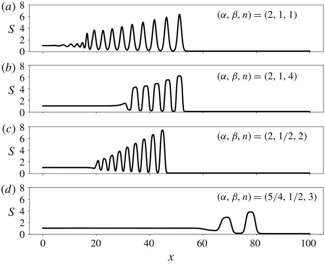
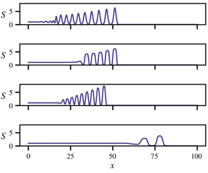
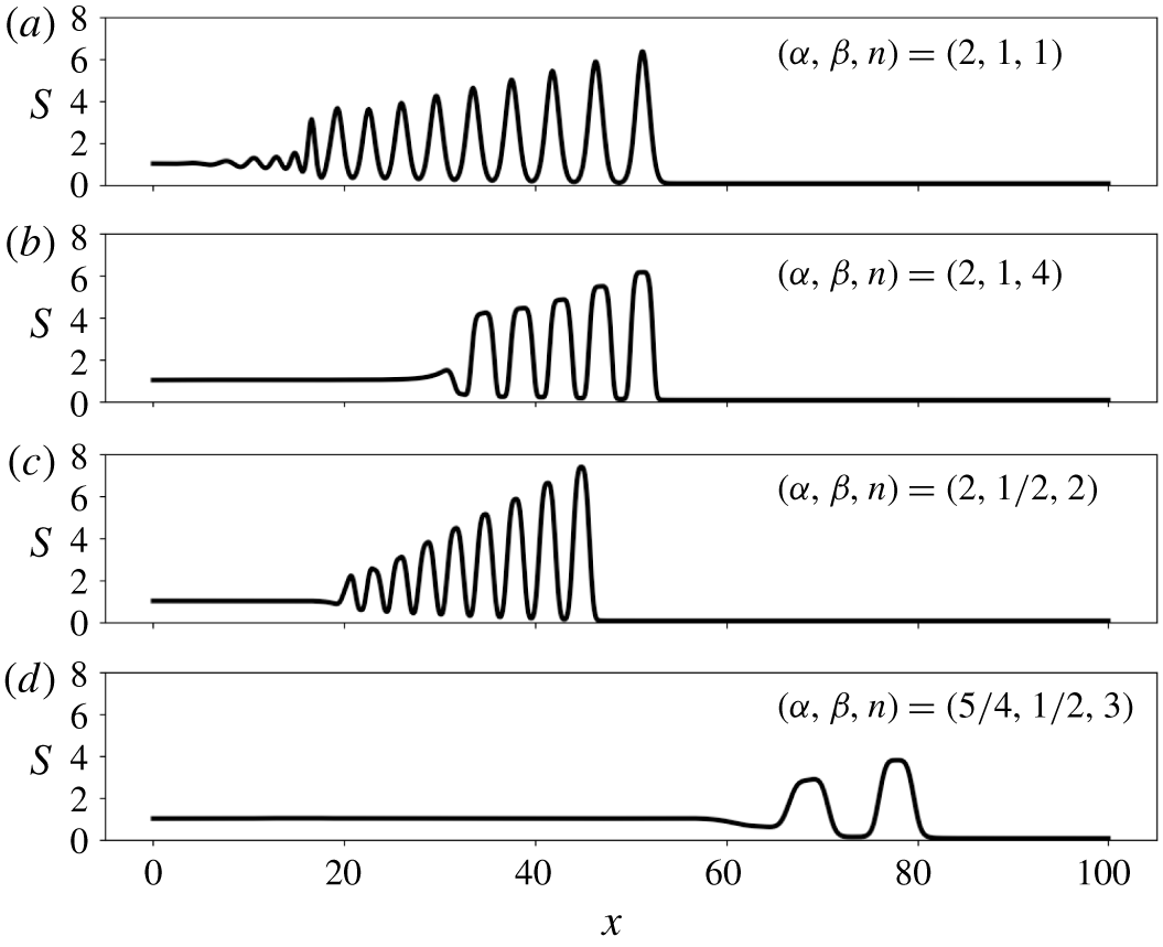
Numerical experiments with initial data provided by (4.8).  $S(x,t)$ is plotted with various parameter choices at time
 $t=75.$ The initial condition is provided by (4.8) with parameters
 $(\unicode[STIX]{x1D70F}_{s},x_{\ast },S_{0})=(10,25,0.05)$. The effect of increasing
 $n$ on wave peak flatness is seen between (a) and (b). Different wave speeds, amplitudes and widths are observed as
 $\unicode[STIX]{x1D6FC}$ and
 $\unicode[STIX]{x1D6FD}$ vary. The rank ordering is lost near the trailing edge of the wave train in (a) (Lowman & Hoefer Reference Lowman and Hoefer2013b). The parameters in (a) are typical in magma dynamics and those in (d) are typical in subglacial hydrology.
Instead of developing into a travelling step shock as predicted by (4.8), a rank-ordered wave train in  $S$ begins to form at
 $t=\unicode[STIX]{x1D70F}_{s}$ for all explored values of
 $(\unicode[STIX]{x1D6FC},n,\unicode[STIX]{x1D6FD})$ demonstrating the dispersive nature of the governing equations (figure 2) (Spiegelman Reference Spiegelman1993b; Lowman & Hoefer Reference Lowman and Hoefer2013b). In a frame moving with the leading
 $S$ wave, we can see from figure 2 that it behaves like a solitary wave in the sense that it travels on the background
 $S_{0}$ with constant speed and permanent shape once it has formed. These dispersive shock waves have been analysed by Lowman & Hoefer (Reference Lowman and Hoefer2013b) in the magma parameter regime and produced in laboratory experiments by Scott et al. (Reference Scott, Stevenson and Whitehead1986) and Maiden et al. (Reference Maiden, Lowman, Anderson, Schubert and Hoefer2016). A related class of periodic waves has also been analysed (Maiden & Hoefer Reference Maiden and Hoefer2016) and produced in experiments (Olson & Christensen Reference Olson and Christensen1986), although these do not decay in amplitude like the dispersive shock waves studied here.
For each  $S$ wave, there is a corresponding
 $N$ wave with a minimum in front of the
 $S$ peak and maximum behind it. The minimum corresponds to fluid overpressure (
 $p_{f}>p_{s}$) that forces the conduit walls in front of the wave to open. Likewise, the maximum corresponds to underpressure (
 $p_{s}>p_{f}$) that forces the conduit walls behind the wave to close. Since these extrema are equal in absolute value but opposite in sign, a self-reinforcing
 $S$ wave is able to propagate.
Numerical experiments show that the wave train associated with subglacial hydrology parameters (figure 3d) differs from the laminar flow examples (figure 3a,b) in wave amplitude, width, peak flatness, speed and frequency. We can also see that the solid rheology controls the flatness of the wave peaks. Increasing the stress exponent  $n$, corresponding to a more plastic matrix, leads to flatter wave peaks. This phenomenon is explored in detail in § 5.2. While the value of
 $n$ has no effect on wave speed in the dimensionless equations, the length scale
 $\tilde{x}$ (3.2) and dimensional wave speed are different for each parameter choice. Further, the rank ordering is lost near the trailing edge of the wave train in the magma parameter regime (figure 3a). Lowman & Hoefer (Reference Lowman and Hoefer2013b) showed that dispersive shock waves eventually ‘implode’ if the initial downstream conduit size
 $S_{0}$ is small enough, as in this case. For the same
 $S_{0}$, the other parameters do not exhibit this behaviour over the same time interval (figure 3b–d).
5 Travelling wave solutions
5.1 Existence of solitary wave solutions
The numerical results point towards the existence of solitary wave solutions to the governing equations (3.3)–(3.5) for a wide range of parameters. Here, we show that they exist for all parameters satisfying the assumptions in (3.6). While we use a phase plane argument below, there is an equivalent variational formulation of the problem (appendix B). Seeking travelling wave solutions, we define  $\unicode[STIX]{x1D709}=x-ct$,
 $c>0$, and make the ansatzes
 $S=S(\unicode[STIX]{x1D709}),N=N(\unicode[STIX]{x1D709})$ and
 $Q=Q(\unicode[STIX]{x1D709})$. Under this assumption, the governing equations reduce to the system of ordinary differential equations
 $$\begin{eqnarray}\displaystyle & \displaystyle c\frac{\text{d}S}{\text{d}\unicode[STIX]{x1D709}}=\frac{\text{d}Q}{\text{d}\unicode[STIX]{x1D709}}, & \displaystyle\end{eqnarray}$$
 $$\begin{eqnarray}\displaystyle & \displaystyle \frac{\text{d}Q}{\text{d}\unicode[STIX]{x1D709}}=S|N|^{n}\text{sgn}(N), & \displaystyle\end{eqnarray}$$
 $$\begin{eqnarray}\displaystyle & \displaystyle \frac{\text{d}N}{\text{d}\unicode[STIX]{x1D709}}=\text{sgn}(Q)|Q|^{1/\unicode[STIX]{x1D6FD}}S^{-(\unicode[STIX]{x1D6FC}/\unicode[STIX]{x1D6FD})}-1. & \displaystyle\end{eqnarray}$$
Equation (5.1) implies that  $cS+\unicode[STIX]{x1D705}=Q$ for some constant
 $\unicode[STIX]{x1D705}$. Seeking solitary wave solutions, we enforce the boundary condition
 $$\begin{eqnarray}\lim _{|\unicode[STIX]{x1D709}|\rightarrow \infty }(S,N,Q)=(1,0,1),\end{eqnarray}$$
which requires that the integration constant  $\unicode[STIX]{x1D705}=1-c$. We set
 $Q=cS+(1-c)$ and substitute this into (5.3) to obtain the following problem that may be studied in the
 $(S,N)$ phase plane:
 $$\begin{eqnarray}\displaystyle & \displaystyle \frac{\text{d}S}{\text{d}\unicode[STIX]{x1D709}}=\frac{1}{c}S|N|^{n}\text{sgn}(N), & \displaystyle\end{eqnarray}$$
 $$\begin{eqnarray}\displaystyle & \displaystyle \frac{\text{d}N}{\text{d}\unicode[STIX]{x1D709}}=\text{sgn}(cS+1-c)|cS+1-c|^{1/\unicode[STIX]{x1D6FD}}S^{-(\unicode[STIX]{x1D6FC}/\unicode[STIX]{x1D6FD})}-1=:P(S;\unicode[STIX]{x1D6FC},\unicode[STIX]{x1D6FD},c). & \displaystyle\end{eqnarray}$$
Solutions to (5.5) and (5.6) that satisfy the boundary condition (5.4) necessarily exist on homoclinic orbits that pass through the fixed point  $(S,N)=(1,0)$. Below, we derive a function
 ${\mathcal{H}}(S,N)$ that is constant on solutions of (5.5)–(5.6). We will show that closed level curves of
 ${\mathcal{H}}$ passing through the point
 $(S,N)=(1,0)$ exist for all parameters satisfying (3.6) when
 $c>\unicode[STIX]{x1D6FC}$. Dividing (5.5) by (5.6) yields the separable equation
 $$\begin{eqnarray}\frac{\text{d}S}{\text{d}N}=\frac{1}{c}\frac{S}{P(S)}\text{sgn}(N)|N|^{n}.\end{eqnarray}$$
We integrate (5.7) to obtain an algebraic relation between  $S$ and
 $N$ in phase space. If they exist, solitary wave solutions satisfy the condition
 ${\mathcal{H}}(S,N)=0$ for
 $$\begin{eqnarray}{\mathcal{H}}(S,N)={\mathcal{I}}_{P}(S)-\frac{1}{c(n+1)}|N|^{n+1},\end{eqnarray}$$
where
 $$\begin{eqnarray}{\mathcal{I}}_{P}(S)=\int _{1}^{S}S_{\ast }^{-1}P(S_{\ast })\,\text{d}S_{\ast }.\end{eqnarray}$$
For our motivating cases  $\unicode[STIX]{x1D6FD}\in \{1,{\textstyle \frac{1}{2}}\}$, analytical expressions for
 ${\mathcal{I}}_{P}$ are given by
 $$\begin{eqnarray}\displaystyle & \displaystyle {\mathcal{I}}_{P}(S)|_{\unicode[STIX]{x1D6FD}=1}=\frac{c}{1-\unicode[STIX]{x1D6FC}}S^{1-\unicode[STIX]{x1D6FC}}-\frac{1-c}{\unicode[STIX]{x1D6FC}}S^{-\unicode[STIX]{x1D6FC}}-\ln (S)+\frac{1-c}{\unicode[STIX]{x1D6FC}}-\frac{c}{1-\unicode[STIX]{x1D6FC}} & \displaystyle\end{eqnarray}$$
 $$\begin{eqnarray}\displaystyle & \displaystyle {\mathcal{I}}_{P}(S)|_{\unicode[STIX]{x1D6FD}=\frac{1}{2}}=\text{sgn}(cS+1-c){\mathcal{I}}_{0}(S)+2{\mathcal{I}}_{0}\left(1-\frac{1}{c}\right)\mathbf{1}_{(0,1-(1/c))}(S)-\ln (S)+C,\qquad & \displaystyle\end{eqnarray}$$
where  $\mathbf{1}_{B}$ is the indicator function for a set
 $B$,
 $$\begin{eqnarray}{\mathcal{I}}_{0}(S)=\frac{c^{2}}{2-2\unicode[STIX]{x1D6FC}}S^{2-2\unicode[STIX]{x1D6FC}}+\frac{2(1-c)c}{1-2\unicode[STIX]{x1D6FC}}S^{1-2\unicode[STIX]{x1D6FC}}-\frac{(1-c)^{2}}{2\unicode[STIX]{x1D6FC}}S^{-2\unicode[STIX]{x1D6FC}},\end{eqnarray}$$
and the integration constant  $C$ is chosen so that
 ${\mathcal{I}}_{P}(1)=0$. Since
 ${\mathcal{H}}$ is continuous and monotonically decreasing in
 $|N|$, the existence of solitary wave solutions is determined by the roots and extrema of
 ${\mathcal{I}}_{P}$;
 $P(1)=0$ implies that a stationary point of
 ${\mathcal{I}}_{P}$ exists at
 $S_{1}=1$ for all
 $c$. For
 $c>\unicode[STIX]{x1D6FC}$ there exists an additional root
 $S_{2}>(c/\unicode[STIX]{x1D6FC})^{1/(\unicode[STIX]{x1D6FC}-1)}>1$ of
 $P$ corresponding to another stationary point of
 ${\mathcal{I}}_{P}$. This can be seen by noting that roots of
 $P(S)$ are roots of the function
 $f(S)=S^{\unicode[STIX]{x1D6FC}}-cS+c-1$. For roots
 $P$, we have that
 $$\begin{eqnarray}{\mathcal{I}}_{P}^{\prime \prime }(S)|_{P(S)=0}=\frac{1}{\unicode[STIX]{x1D6FD}S^{2}}(cS^{1-\unicode[STIX]{x1D6FC}}-\unicode[STIX]{x1D6FC}).\end{eqnarray}$$
For  $c>\unicode[STIX]{x1D6FC}$,
 ${\mathcal{I}}^{\prime \prime }(1)>0$ and
 ${\mathcal{I}}^{\prime \prime }(S_{2})<0$. Since
 ${\mathcal{I}}_{P}\rightarrow -\infty$ as
 $S\rightarrow \infty$, this implies that there exists a second root
 $A>S_{2}$ of
 ${\mathcal{I}}_{P}$. Therefore, there exists a closed curve in phase space connecting
 $(1,0)$ and
 $(A,0)$ when
 $c>\unicode[STIX]{x1D6FC}$. Solitary wave solutions with amplitude
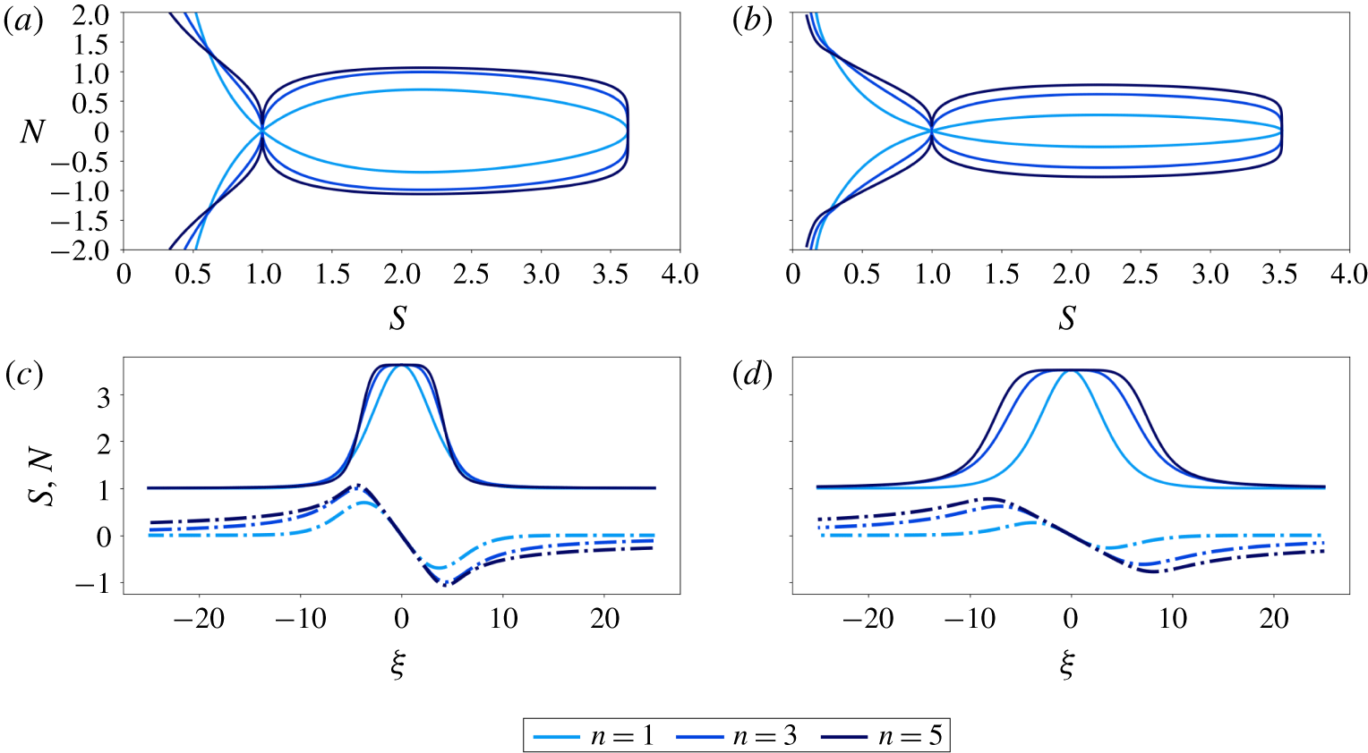
 $A$ exist on this homoclinic orbit (figure 4). For
 $c<\unicode[STIX]{x1D6FC}$, the second root of
 $P$ satisfies
 $S_{2}<1$ and
 ${\mathcal{I}}_{P}^{\prime \prime }(1)<0$. Therefore, when
 $c<\unicode[STIX]{x1D6FC}$ there is no root
 $A>1$ of
 ${\mathcal{I}}_{P}$ and no solitary waves exist. Thus, the solitary wave speed is bounded below by
 $\unicode[STIX]{x1D6FC}$.
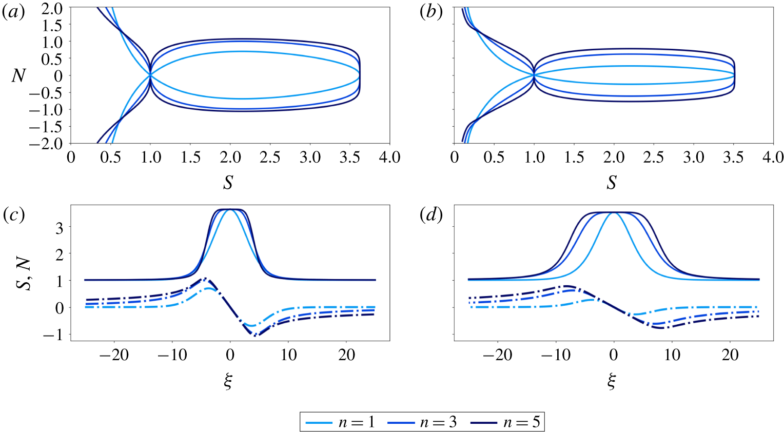
Panels (a,b) show how the shape of the homoclinic orbits change as  $n$ is varied for fixed
 $(\unicode[STIX]{x1D6FC},\unicode[STIX]{x1D6FD},c)$. Homoclinic orbits are the level curves
 ${\mathcal{H}}(S,N)=0$, as defined in (5.8). Analytical expressions for
 ${\mathcal{I}}_{P}$ are given by (5.10) for (a) and (5.11)–(5.12) for (b). Panels (c,d) show solutions of the system (5.5)–(5.6) for various values of
 $n$, integrated from
 $\unicode[STIX]{x1D709}=0$ to
 $|\unicode[STIX]{x1D709}|=25$ with initial condition
 $(S(0),N(0))=(A,0)$.
 $S$ is solid and
 $N$ is dashed. For (a,c) the wave speed is
 $c=3.15$ and the parameter choices
 $(\unicode[STIX]{x1D6FC},\unicode[STIX]{x1D6FD})=(2,1)$ correspond to laminar pipe flow. For (b,d), the wave speed is
 $c=1.4$ and the parameter choices
 $(\unicode[STIX]{x1D6FC},\unicode[STIX]{x1D6FD})=(1.25,0.5)$ correspond to the Darcy–Weisbach law for turbulent pipe flow. These wave speeds are chosen so that the amplitudes of the turbulent and laminar waves are approximately the same.
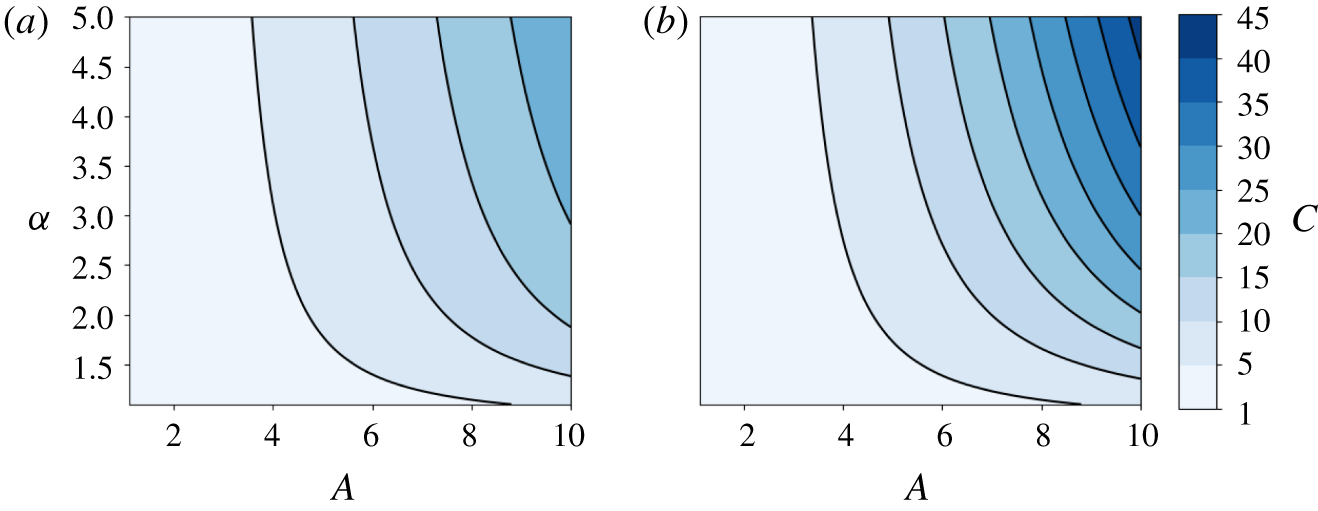
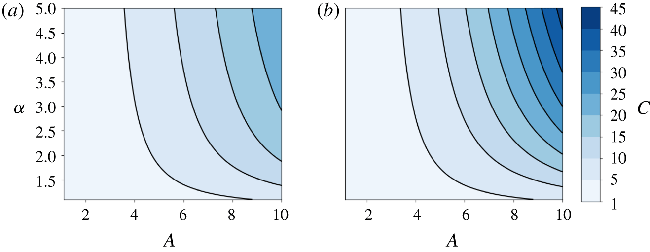
Dispersion relations for (a) turbulent ( $\unicode[STIX]{x1D6FD}={\textstyle \frac{1}{2}}$) and (b) laminar (
 $\unicode[STIX]{x1D6FD}=1$) flow. For the same
 $A$ and
 $\unicode[STIX]{x1D6FC}$, the laminar waves always travel faster than the turbulent waves.
We obtain dispersion relations from the condition
 $$\begin{eqnarray}{\mathcal{I}}_{P}(A;\unicode[STIX]{x1D6FC},\unicode[STIX]{x1D6FD},c)=0.\end{eqnarray}$$
For  $\unicode[STIX]{x1D6FD}=1$, we solve (5.14) for
 $c$ and obtain
 $$\begin{eqnarray}c(A,\unicode[STIX]{x1D6FC})|_{\unicode[STIX]{x1D6FD}=1}=\frac{(\unicode[STIX]{x1D6FC}-1)(\unicode[STIX]{x1D6FC}A^{\unicode[STIX]{x1D6FC}}\ln (A)-A^{\unicode[STIX]{x1D6FC}}+1)}{A^{\unicode[STIX]{x1D6FC}}-\unicode[STIX]{x1D6FC}A+\unicode[STIX]{x1D6FC}-1}.\end{eqnarray}$$
Equation (5.15) is equivalent to equation (8) of Scott & Stevenson (Reference Scott and Stevenson1984). Dispersion relations can be obtained numerically for general  $\unicode[STIX]{x1D6FD}$. The wave speed is an increasing function of
 $A$ and
 $\unicode[STIX]{x1D6FC}$ for both laminar and turbulent flows, although the dependence is weaker in the latter (figure 5). Thus, solitary waves travel slower in the turbulent flow regime than in the laminar flow regime. This explains the discrepancy in wave speed between the laminar (figure 3a,b) and turbulent (figure 3c) flow experiments explored in the previous section. From (5.14) we see that the non-dimensional wave speed does not depend on the stress exponent
 $n$. We observed this numerically in figure 3(a,b) as the leading waves travelled at the same speed for different values of
 $n$. However, we note that the dimensional wave speed depends on
 $n$ indirectly through the length scale
 $\tilde{x}$ in (3.2).
To find solitary wave profiles, we solve for  $N(S)$ on the homoclinic orbit (where
 ${\mathcal{H}}=0$) and integrate (5.5) to obtain the implicit relation
 $$\begin{eqnarray}\unicode[STIX]{x1D709}(S)=\int _{S}^{A}S_{\star }^{-1}c[c(n+1){\mathcal{I}}_{P}(S_{\star })]^{-n/(n+1)}\,\text{d}S_{\star },\end{eqnarray}$$
where we have assumed that  $\unicode[STIX]{x1D709}>0$. Solitary wave profiles can be computed directly from (5.16) by quadrature. Example profiles are shown in figure 4.
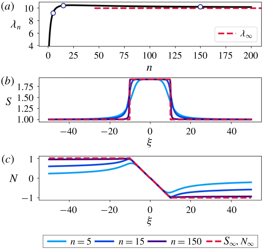
We define the half-width  $\unicode[STIX]{x1D706}_{n}$ of a wave for any given
 $n>0$ as the location of the absolute maximum in pressure,
 $$\begin{eqnarray}\unicode[STIX]{x1D706}_{n}:=\text{arg max}_{\unicode[STIX]{x1D709}>0}|N(\unicode[STIX]{x1D709})|=\unicode[STIX]{x1D709}(S_{2};n),\end{eqnarray}$$
where  $\unicode[STIX]{x1D709}(S)$ is defined in (5.16). Equation (5.17) follows from
 $|N|$ being maximized at
 $S=S_{2}$ in phase space.
5.2 Asymptotically square waves
Numerical results show that the flatness of the  $S$ wave peaks increases with the stress exponent
 $n$ (figures 3 and 4). In the perfectly plastic limit
 $n\rightarrow \infty$, these solutions approach square waves asymptotically. We evaluate (5.16) at an arbitrary
 ${\hat{S}}\in (1,A)$ and make the change of variables
 $u={\mathcal{I}}_{P}$. Furthermore, we define
 $\unicode[STIX]{x1D700}=(n+1)^{-1}$. Then, equation (5.16) becomes
 $$\begin{eqnarray}\unicode[STIX]{x1D709}({\hat{S}};\unicode[STIX]{x1D700})=\int _{0}^{u({\hat{S}})}\frac{c^{\unicode[STIX]{x1D700}}(u/\unicode[STIX]{x1D700})^{\unicode[STIX]{x1D700}-1}}{P({\mathcal{I}}_{P}^{-1}(u))}\,\text{d}u.\end{eqnarray}$$
Integration by parts shows that the function  ${\textstyle \frac{1}{2}}|u/\unicode[STIX]{x1D700}|^{\unicode[STIX]{x1D700}-1}$ converges to the Dirac delta in the distributional sense as
 $\unicode[STIX]{x1D700}\rightarrow 0$ (
 $n\rightarrow \infty$). Therefore, we have that
 $$\begin{eqnarray}\lim _{\unicode[STIX]{x1D700}\rightarrow 0}\unicode[STIX]{x1D709}({\hat{S}};\unicode[STIX]{x1D700})=\frac{1}{|P(A)|}=:\unicode[STIX]{x1D706}_{\infty }\end{eqnarray}$$
for all  ${\hat{S}}\in (1,A)$. Since
 $S$ is bounded above by
 $A$, below by
 $1$ and is continuous for every
 $n>0$, this implies that
 $$\begin{eqnarray}S_{\infty }(\unicode[STIX]{x1D709}):=\lim _{n\rightarrow \infty }S(\unicode[STIX]{x1D709};n)=\left\{\begin{array}{@{}ll@{}}A\quad & |\unicode[STIX]{x1D709}|<\unicode[STIX]{x1D706}_{\infty },\\ 1\quad & |\unicode[STIX]{x1D709}|>\unicode[STIX]{x1D706}_{\infty }.\end{array}\right.\end{eqnarray}$$
We see that  $\unicode[STIX]{x1D706}_{\infty }=\lim _{n\rightarrow \infty }\unicode[STIX]{x1D706}_{n}$ so that our definition of wave half-width in (5.17) is consistent with the true half-width in the limit of a perfectly plastic matrix. Given the limiting behaviour of
 $S$, we determine from (5.6) that in the limit
 $n\rightarrow \infty$,
 $N$ approaches the ramp function
 $$\begin{eqnarray}N_{\infty }(\unicode[STIX]{x1D709})=\left\{\begin{array}{@{}ll@{}}-{\displaystyle \frac{1}{\unicode[STIX]{x1D706}_{\infty }}}\unicode[STIX]{x1D709}\quad & |\unicode[STIX]{x1D709}|\leqslant \unicode[STIX]{x1D706}_{\infty },\\ \text{sgn}(-\unicode[STIX]{x1D709})\quad & |\unicode[STIX]{x1D709}|>\unicode[STIX]{x1D706}_{\infty }.\end{array}\right.\end{eqnarray}$$
Solitary wave solutions may be well approximated by  $S_{\infty }$ and
 $N_{\infty }$ for large
 $n$. Furthermore,
 $\unicode[STIX]{x1D706}_{n}$ approaches
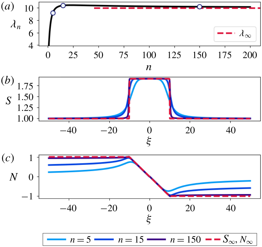
 $\unicode[STIX]{x1D706}_{\infty }$ rather quickly (figure 6). However, the approximation for
 $N$ is only accurate near the origin since
 $N_{\infty }$ does not satisfy the boundary condition (5.4). Equations (5.6) and (5.19) show that waves associated with turbulent flow (
 $\unicode[STIX]{x1D6FD}={\textstyle \frac{1}{2}}$) will be wider than those associated with laminar flow (
 $\unicode[STIX]{x1D6FD}=1$) for the same value of
 $\unicode[STIX]{x1D6FC}$ (figure 4). These results establish
 $\unicode[STIX]{x1D706}_{\infty }$ as a useful approximation of wave half-width in the case of a nearly plastic matrix.
(a) The wave half-width  $\unicode[STIX]{x1D706}_{n}$ from (5.16) and (5.17) is computed for
 $n\in [1,200]$ by quadrature with the parameter choice
 $(\unicode[STIX]{x1D6FC},\unicode[STIX]{x1D6FD},c)=(2,{\textstyle \frac{1}{2}},2.5)$. Dashed line corresponds to
 $\unicode[STIX]{x1D706}_{\infty }$. Points on the curve correspond to
 $n$ values shown in (b,c). (b) Plots of
 $S$ as
 $n$ increases, along with the square wave
 $S_{\infty }$. (c) Plots of
 $N$ as
 $n$ increases, along with the ramp function
 $N_{\infty }$.
6 The effect of discharge-dependent melting
In our search for solitary wave solutions, we neglected the effect of phase change on conduit evolution. Melting of ice at the conduit walls is always included in models of subglacial channel evolution (Röthlisberger Reference Röthlisberger1972; Nye Reference Nye1976; Fowler Reference Fowler1999; Clarke Reference Clarke2003; Hewitt et al. Reference Hewitt, Schoof and Werder2012). In this case, the dimensional governing equations (2.2)–(2.3) for channel evolution are modified to
 $$\begin{eqnarray}\displaystyle & \displaystyle \frac{\unicode[STIX]{x2202}S}{\unicode[STIX]{x2202}t}=-\frac{\unicode[STIX]{x2202}Q}{\unicode[STIX]{x2202}x}+\frac{1}{\unicode[STIX]{x1D70C}_{f}l}Q\left(\unicode[STIX]{x1D713}_{0}+\frac{\unicode[STIX]{x2202}N}{\unicode[STIX]{x2202}x}\right), & \displaystyle\end{eqnarray}$$
 $$\begin{eqnarray}\displaystyle & \displaystyle \frac{\unicode[STIX]{x2202}Q}{\unicode[STIX]{x2202}x}=KS|N|^{n}\text{sgn}(N)-\frac{\unicode[STIX]{x1D70C}_{f}-\unicode[STIX]{x1D70C}_{s}}{\unicode[STIX]{x1D70C}_{f}\unicode[STIX]{x1D70C}_{s}l}Q\left(\unicode[STIX]{x1D713}_{0}+\frac{\unicode[STIX]{x2202}N}{\unicode[STIX]{x2202}x}\right), & \displaystyle\end{eqnarray}$$
where  $l$ is the latent heat,
 $\unicode[STIX]{x1D70C}_{f}$ is the fluid density and
 $\unicode[STIX]{x1D70C}_{s}$ is the solid density (Nye Reference Nye1976). The melt rate, proportional to
 $Q(\unicode[STIX]{x1D713}_{0}+(\unicode[STIX]{x2202}N/\unicode[STIX]{x2202}x))$, is derived by neglecting heat advection and assuming that the fluid in the channel and the solid at the channel walls are always at the melting point (Nye Reference Nye1976). We non-dimensionalize (6.1)–(6.2) using the scaling in (3.1)–(3.2). After dropping primes on the dimensionless variables, equations (6.1)–(6.2) become
 $$\begin{eqnarray}\displaystyle & \displaystyle \frac{\unicode[STIX]{x2202}S}{\unicode[STIX]{x2202}t}=-\frac{\unicode[STIX]{x2202}Q}{\unicode[STIX]{x2202}x}+mQ\left(1+\frac{\unicode[STIX]{x2202}N}{\unicode[STIX]{x2202}x}\right), & \displaystyle\end{eqnarray}$$
 $$\begin{eqnarray}\displaystyle & \displaystyle \frac{\unicode[STIX]{x2202}Q}{\unicode[STIX]{x2202}x}=S|N|^{n}\text{sgn}(N)-\left(\frac{\unicode[STIX]{x1D70C}_{f}}{\unicode[STIX]{x1D70C}_{s}}-1\right)mQ\left(1+\frac{\unicode[STIX]{x2202}N}{\unicode[STIX]{x2202}x}\right), & \displaystyle\end{eqnarray}$$
where we have defined the dimensionless melt rate parameter
 $$\begin{eqnarray}\displaystyle m=\frac{{\tilde{N}}}{\unicode[STIX]{x1D70C}_{f}l}. & & \displaystyle\end{eqnarray}$$
In the limit  $m\rightarrow 0$, equations (6.3)–(6.4) reduce to (3.3)–(3.4). The equation for the discharge
 $Q$ (3.5) remains unchanged. Solutions to (6.3)–(6.4) and (3.5) exhibit wave-like behaviour for the non-zero values of
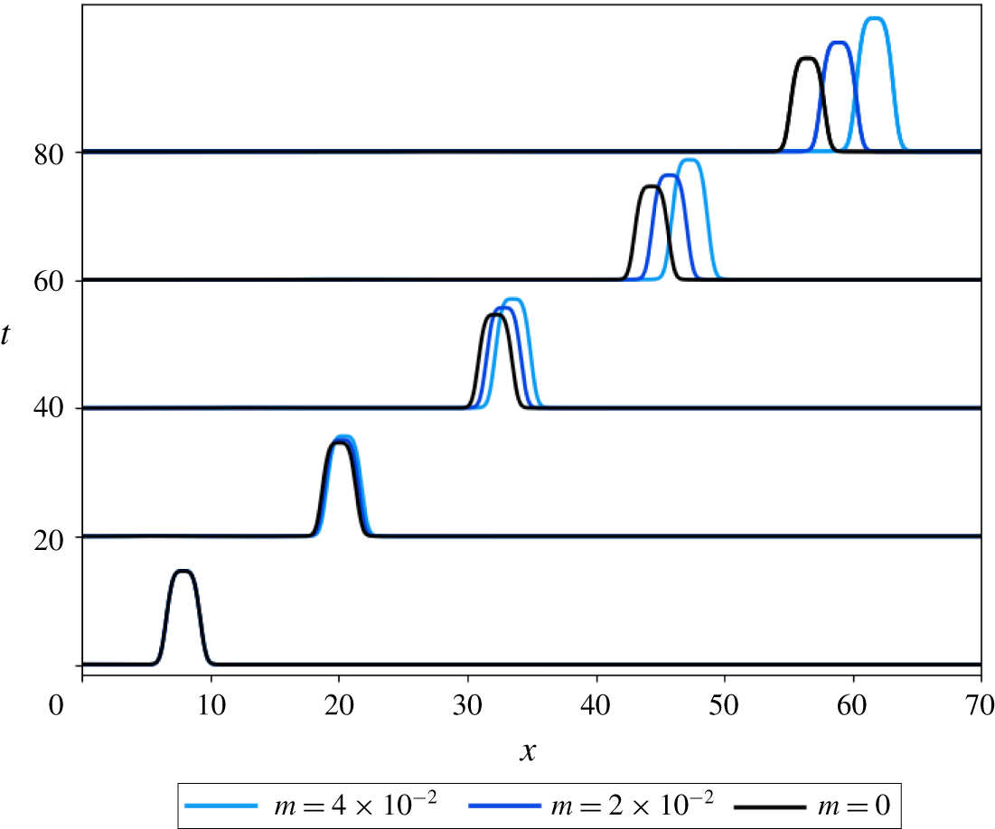
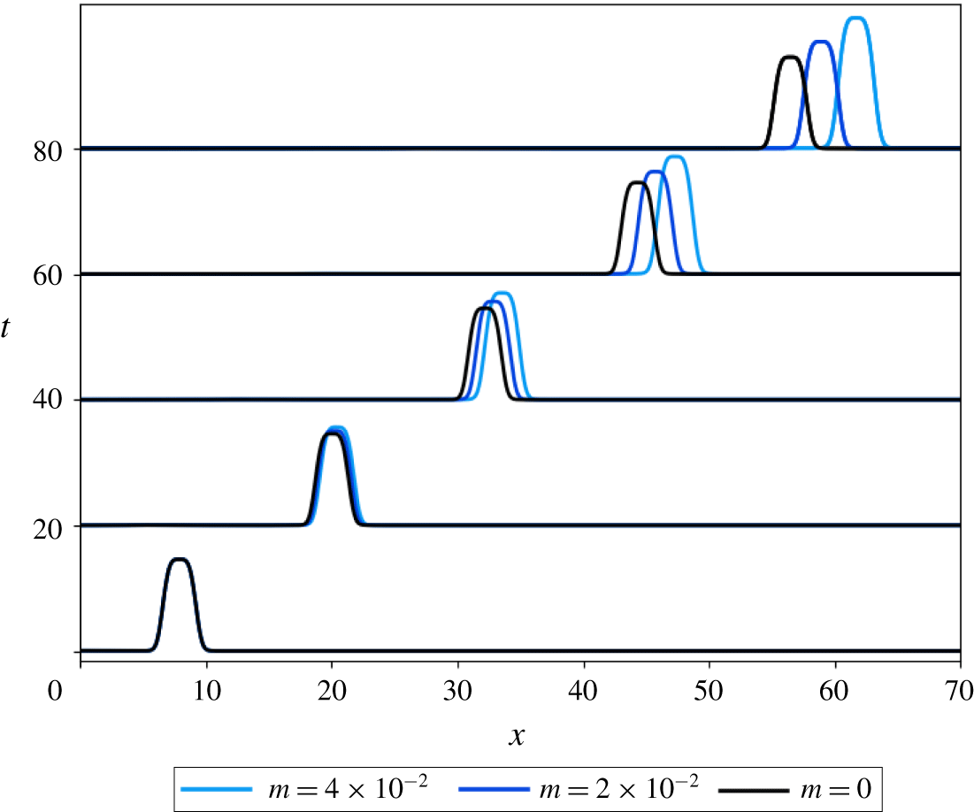
 $m$ explored here. To demonstrate this numerically, we study the evolution of a solitary wave solution to the
 $m=0$ equations for some positive values of
 $m$ (figure 7). The waves with melting included resemble the solitary wave except that they grow and accelerate over time. This phenomenon is a result of the feedbacks among discharge, melting, channel size and dispersion. Melting is strongest at the wave peak where discharge is large. Concentration of melting at the peak leads to a growth in amplitude. This in turn causes the wave to travel more quickly due to the dispersion relation discussed in the previous section (figure 5). We find that solutions with larger
 $m$ grow and accelerate more rapidly (figure 7). In the magma equations, Spiegelman (Reference Spiegelman1993b) found that a uniform melt rate can lead to damping of the waves as the background porosity grows. We expect that damping will also occur in this model if the background conduit size becomes large enough. This scenario can be expected if either the initial background conduit size
 $S_{0}$ or melt rate parameter
 $m$ is sufficiently large because the melt rate is
 ${\sim}mS_{0}^{\unicode[STIX]{x1D6FC}}$ away from the wave peak.
Numerical solution of (6.3)–(6.4) and (3.5) for two choices of positive melt rate parameter  $m$ (blue) compared to the no-melting case where
 $m=0$ (black). We set
 $\unicode[STIX]{x1D70C}_{f}/\unicode[STIX]{x1D70C}_{s}-1=0.1$ in (6.4) for all examples and choose the parameters
 $(\unicode[STIX]{x1D6FC},\unicode[STIX]{x1D6FD},n)=({\textstyle \frac{5}{4}},{\textstyle \frac{1}{2}},3)$. The initial condition is a solitary wave solution to the
 $m=0$ equations with amplitude
 ${\sim}4.8$ and background conduit size
 $S_{0}=0.005$. The solution with larger
 $m$ (light blue) grows and accelerates faster than the one with smaller
 $m$ (dark blue). The
 $m>0$ solutions remain localized like the
 $m=0$ solution.
7 Discussion
The governing equations (3.3)–(3.5) describe a broad class of models for fluid flow through deformable conduits with a wide range of geophysical applications. We have shown that solitary wave solutions and dispersive shock waves are a common feature of models described by these equations. While similar solutions have received much attention in the magma dynamics community, their presence has only recently been discussed in subglacial hydrology (Meyer et al. Reference Meyer, Hewitt and Neufeld2017) even though the governing equations were derived decades ago by Nye (Reference Nye1976). Moreover, since nearly all subglacial hydrology models are related to these governing equations, solitary wave-like solutions are expected to be a common feature of these models.
Solitary wave solutions are a natural consequence of fluid flow in viscously deformable media. It is less obvious whether they should manifest in natural systems. For example, a typical parameter set in subglacial hydrology is  $\unicode[STIX]{x1D6FE}=0.1~\text{Pa}^{-(1/2)}~\text{s}^{-1}~\text{m}$,
 $K=10^{-24}~\text{Pa}^{-n}~\text{s}^{-1}$,
 $\unicode[STIX]{x1D713}_{0}=100~\text{Pa}~\text{m}^{-1}$,
 $\tilde{S}=1~\text{m}^{2}$,
 $\unicode[STIX]{x1D6FD}={\textstyle \frac{1}{2}}$,
 $n=3$ and
 $\unicode[STIX]{x1D6FC}=5/4$. These quantities lead to a length scale of
 $\tilde{x}\approx 30~\text{km}$. From figure 4(d), we see that the wave half-width for
 $\unicode[STIX]{x1D6FD}={\textstyle \frac{1}{2}}$ and
 $n=3$ is
 $\unicode[STIX]{x1D706}_{3}|_{\unicode[STIX]{x1D6FD}={\textstyle \frac{1}{2}}}\approx 10$ so that the dimensional wave half-width is
 ${\sim}300~\text{km}$. It is unlikely that a channel long enough to support such a solitary wave exists beneath the Greenland or Antarctic ice sheets (Chandler et al. Reference Chandler, Wadham, Lis, Cowton, Sole, Bartholomew, Telling, Nienow, Bagshaw and Mair2013; Siegfried et al. Reference Siegfried, Fricker, Carter and Tulaczyk2016). This unreasonably large length scale may be the reason behind the lack of discussion of these waves in the context of subglacial hydrology. Even if the waves were of a reasonable scale, the necessary condition of a persistent fluid overpressure is also unlikely because this would cause separation between the ice and bed, leading to leakage of water out of the channel (Hewitt et al. Reference Hewitt, Schoof and Werder2012). Even so, the observations by Adhikari et al. (Reference Adhikari, Ivins and Larour2017) provide a motivating example of where solitary waves may be important in glaciology. However, our results suggest it is unlikely that the observed wave was related to a solitary wave in a subglacial channel.
The original model from Nye (Reference Nye1976) allows mass transfer between water in the conduit and the surrounding ice. Phase change drives many important processes in subglacial hydrology such as glacial outburst floods (Fowler Reference Fowler1999) and freezing of ice to the base of the ice sheets (Creyts & Clarke Reference Creyts and Clarke2010; Bell et al. Reference Bell, Ferraccioli, Creyts, Braaten, Corr, Das, Damaske, Frearson, Jordan and Rose2011, Reference Bell, Tinto, Das, Wolovick, Chu, Creyts, Frearson, Abdi and Paden2014). We have shown numerically that solitary wave-like solutions also exist when a discharge-dependent melt rate is included, although the waves grow and accelerate over time (figure 7). A further generalization of the model would be to consider a viscoelastic solid rheology, although elasticity is typically neglected in subglacial hydrology. Solitary waves in viscoelastic porous media have been explored previously and may be relevant in shallow magmatic systems (Grimshaw, Helfrich & Whitehead Reference Grimshaw, Helfrich and Whitehead1992; Connolly & Podladchikov Reference Connolly and Podladchikov1998; Yarushina, Podladchikov & Connolly Reference Yarushina, Podladchikov and Connolly2015).
The solitary wave solutions explored here may be used as time-dependent benchmark solutions for code verification in a wide range of settings. Previous studies have demonstrated the utility of solitary wave solutions as computational benchmarks in magma dynamics since one only needs to measure the change in speed and shape of the wave over time (Simpson & Spiegelman Reference Simpson and Spiegelman2011; Keller, May & Kaus Reference Keller, May and Kaus2013). Since the governing equations (2.2)–(2.4) are closely related to nearly all subglacial hydrology models, these solutions may be widely applicable as computational benchmarks. We provide example benchmark tests and convergence results in the appendix A.
A previously unrecognized feature of (3.3)–(3.5) is the rheology-dependent flattening property: increasing the stress exponent  $n$, corresponding to a more plastic matrix, results in flatter
 $S$ wave peaks. The property is robust in the sense that it holds true for any choice of parameters (
 $\unicode[STIX]{x1D6FC},\unicode[STIX]{x1D6FD}$) and results in asymptotically square waves in the limit of a perfectly plastic matrix. Laboratory experiments with shear-thinning fluids would be useful in testing the physical veracity of this property.
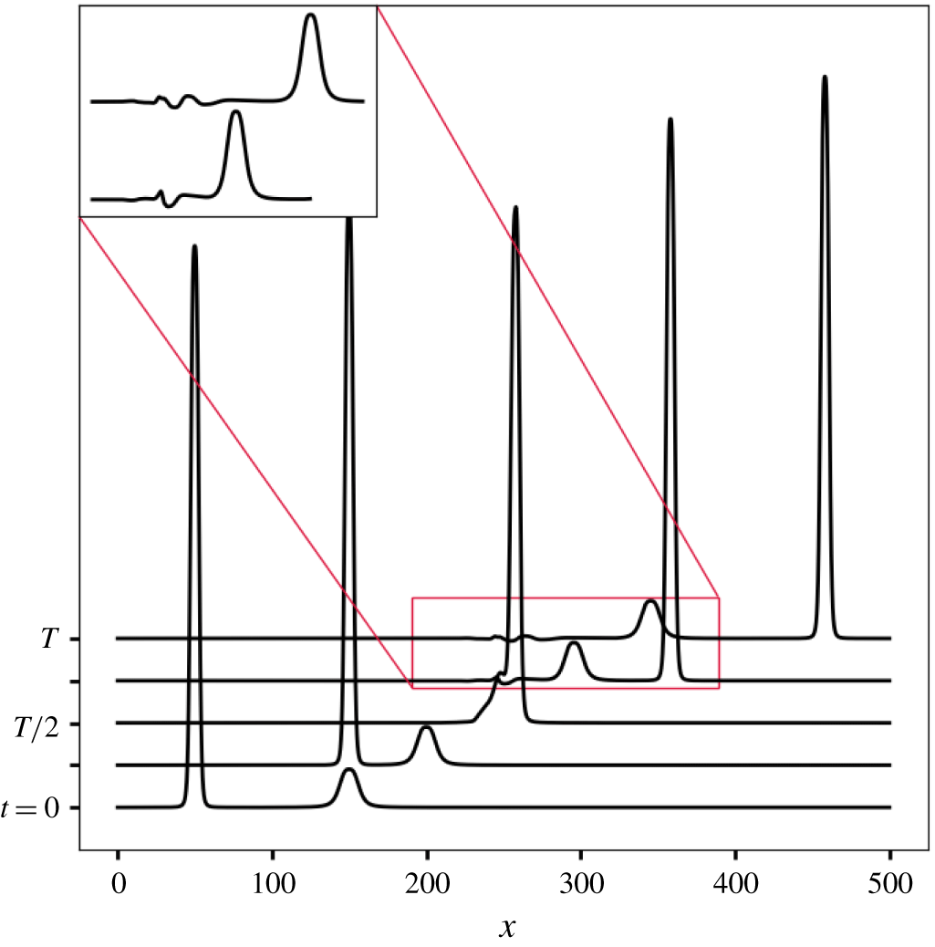
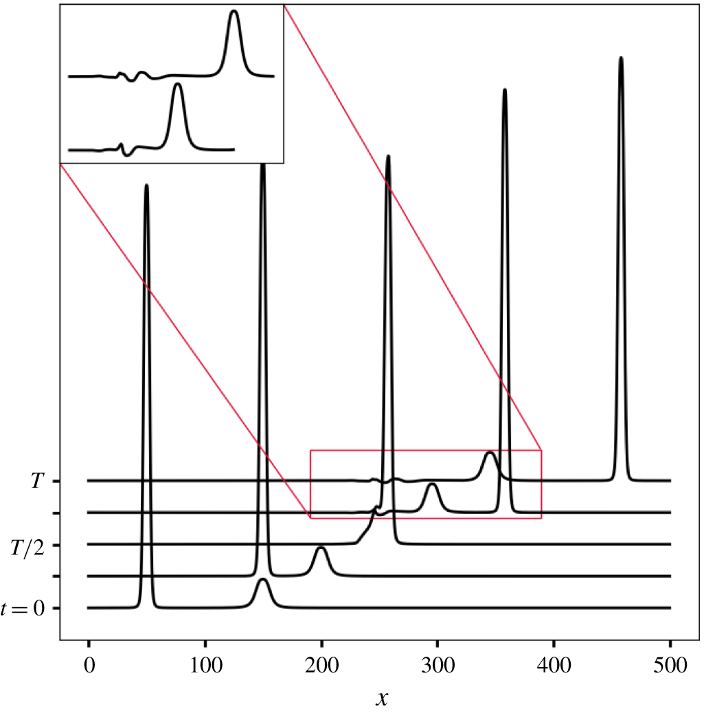
Asymptotic stability of solitary wave solutions to the magma equation (3.8) has been established by Simpson & Weinstein (Reference Simpson and Weinstein2008). We expect that the solitary waves explored here are also dynamically stable. In numerical experiments we observe that solitary waves are preserved after collision, although a small dispersive tail is generated behind the slower wave (figure 8). Energy loss during solitary wave collision has previously been observed in the  $(\unicode[STIX]{x1D6FC},\unicode[STIX]{x1D6FD},n)=(2,1,1)$ case (Lowman et al. Reference Lowman, Hoefer and El2014) and in the closely related magma equation (3.8) (Barcilon & Richter Reference Barcilon and Richter1986), indicating that these solutions are not solitons. Rigorous investigation of nonlinear stability of the solitary waves is left for future work.
Numerical experiment of two solitary waves colliding. We choose the parameters  $(\unicode[STIX]{x1D6FC},\unicode[STIX]{x1D6FD},n)=(2,1,2)$ and wave speeds
 $c={\textstyle \frac{5}{2}}$ (shorter) and 5 (taller). The final time is
 $T=80$ and the solution is plotted in increments of
 $T/4$. We choose a mesh spacing
 $h={\textstyle \frac{1}{20}}$ and time step
 $\unicode[STIX]{x0394}t={\textstyle \frac{1}{400}}$. A dispersive tail is generated behind the waves after collision. The inset provides a closer view of the dispersive tail.
Acknowledgements
A.G.S. thanks J. Kingslake for discussion regarding glaciological applications of these results. Partial support for this work was provided by NSF EAR-1520732 (M.S.) and a graduate fellowship from Columbia University’s Department of Earth and Environmental Sciences (A.G.S.). T.T.C. was supported by a Vetlesen Foundation grant, NSF-1643970 and NASA-NNX16AJ95G.
Declaration of interests
The authors report no conflict of interest.
Appendix A. Finite element method
Here, we outline a finite element method for solving the non-dimensional governing equations (3.3)–(3.5) with  $x\in [0,L]$ and
 $t\in [0,T]$. We make the spatial approximation
 $(S(\cdot ,t),N(\cdot ,t),Q(\cdot ,t))\in (\mathbb{P}_{2}\times \mathbb{P}_{1}\times \mathbb{P}_{2})$ for all
 $t\in [0,T]$, where
 $\mathbb{P}_{1}$ and
 $\mathbb{P}_{2}$ are the spaces of piecewise linear and quadratic functions, respectively. We define the homogeneous subspaces
 $$\begin{eqnarray}\mathbb{P}_{k,0}=\{p\in \mathbb{P}_{k}|\;p(0)=0\},\end{eqnarray}$$
to account for Dirichlet boundary conditions on  $(S,N,Q)$ at
 $x=0$. Multiplying (3.3)–(3.5) by test functions
 $(\unicode[STIX]{x1D711}_{S},\unicode[STIX]{x1D711}_{N},\unicode[STIX]{x1D711}_{Q})\in (\mathbb{P}_{2,0}\times \mathbb{P}_{1,0}\times \mathbb{P}_{2,0})$ and integrating generates the weak forms
 $$\begin{eqnarray}\displaystyle & \displaystyle F_{1}=\int _{0}^{L}\left[\frac{\unicode[STIX]{x2202}S}{\unicode[STIX]{x2202}t}+S|N|^{n}\text{sgn}(N)\right]\unicode[STIX]{x1D711}_{S}\,\text{d}x, & \displaystyle\end{eqnarray}$$
 $$\begin{eqnarray}\displaystyle & \displaystyle F_{2}=\int _{0}^{L}S|N|^{n}\text{sgn}(N)\unicode[STIX]{x1D711}_{N}\,\text{d}x+\int _{0}^{L}\!Q\frac{\unicode[STIX]{x2202}\unicode[STIX]{x1D711}_{N}}{\unicode[STIX]{x2202}x}\,\text{d}x-[Q\unicode[STIX]{x1D711}_{N}]_{x=L}, & \displaystyle\end{eqnarray}$$
 $$\begin{eqnarray}\displaystyle & \displaystyle F_{3}=\int _{0}^{L}[Q-S^{\unicode[STIX]{x1D6FC}}\unicode[STIX]{x1D6F9}|\unicode[STIX]{x1D6F9}|^{\unicode[STIX]{x1D6FD}-1}]\unicode[STIX]{x1D711}_{Q}\,\text{d}x, & \displaystyle\end{eqnarray}$$
where  $\unicode[STIX]{x1D6F9}=1+\unicode[STIX]{x2202}N/\unicode[STIX]{x2202}x.$ We integrated the left side of (3.4) by parts and the boundary term
 $[Q\unicode[STIX]{x1D711}_{N}]_{x=0}$ vanished because
 $\unicode[STIX]{x1D711}_{N}\in \mathbb{P}_{1,0}.$ We define
 $F=F_{1}+F_{2}+F_{3}$ and solve the nonlinear variational problem
 $$\begin{eqnarray}F(S,N,Q;\unicode[STIX]{x1D711}_{S},\unicode[STIX]{x1D711}_{N},\unicode[STIX]{x1D711}_{Q})=0\end{eqnarray}$$
using the finite element package FEniCS (Logg et al. Reference Logg, Mardal and Wells2012; Alnaes et al. Reference Alnæs, Blechta, Hake, Johansson, Kehlet, Logg, Richardson, Ring, Rognes and Wells2015). We integrate (A 2) in time with the trapezoidal rule. The boundary conditions are described in the main text (§ 4). Convergence of the numerical scheme is detailed in figures 9 and 10, following the approach of Simpson & Spiegelman (Reference Simpson and Spiegelman2011).
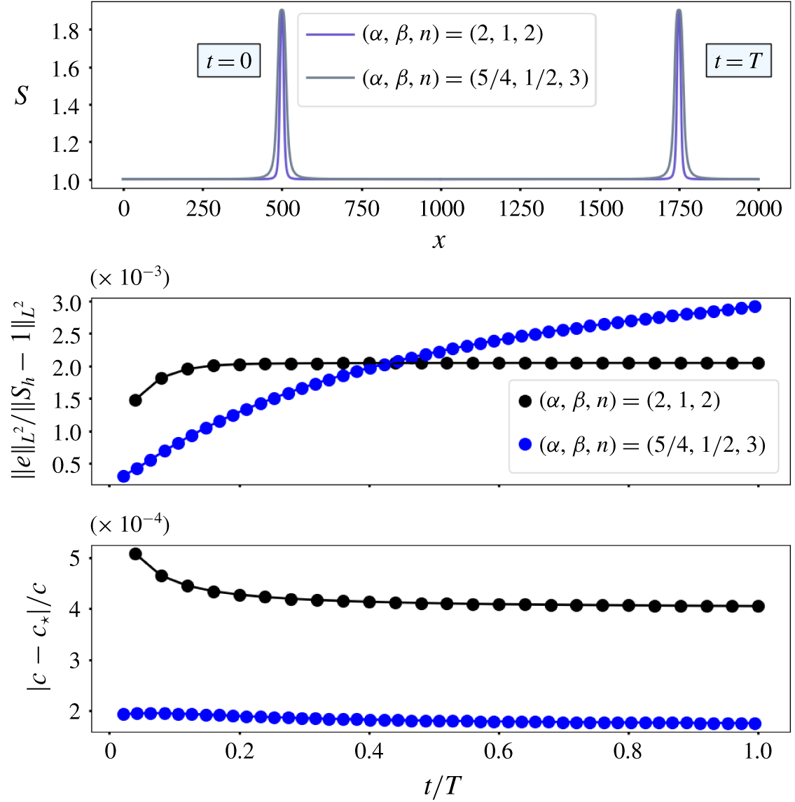
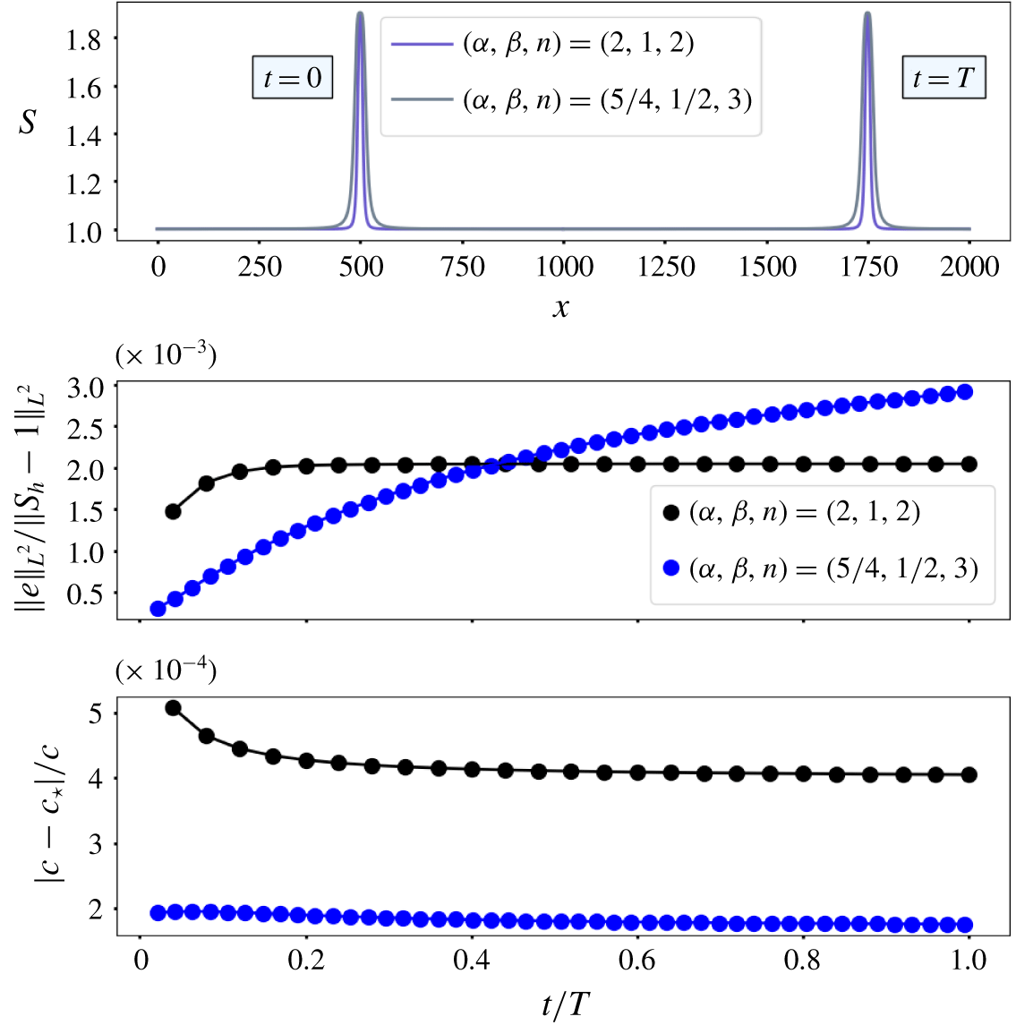
Numerical solution of (3.3)–(3.5) with solitary wave solutions  $S_{a}(\unicode[STIX]{x1D709})$ of (5.1)–(5.3) provided as initial conditions. The numerical scheme is given in appendix A. The parameters chosen are
 $(\unicode[STIX]{x1D6FC},\unicode[STIX]{x1D6FD},n,c)=(2,1,2,{\textstyle \frac{5}{2}})$ for laminar flow and
 $(\unicode[STIX]{x1D6FC},\unicode[STIX]{x1D6FD},n,c)=({\textstyle \frac{5}{4}},{\textstyle \frac{1}{2}},3,1.3223)$ for turbulent flow. The domain length is
 $L=2000$. The initial condition travels with nearly constant speed and shape until the final time
 $T=500$ for laminar flow and
 $T=945$ for turbulent flow. The time step
 $\unicode[STIX]{x0394}t$ is chosen so that
 $c\unicode[STIX]{x0394}t/h={\textstyle \frac{1}{2}}$ where
 $h={\textstyle \frac{1}{2}}$ is the mesh spacing and
 $S_{h}$ is the associated numerical solution. We plot the relative speed error
 $|c-c_{\star }|/c$ over time, where the numerical wave speed
 $c_{\star }$ minimizes the shape error
 $\Vert S_{a}(x-c_{\star }t)-S_{h}(x,t)\Vert _{L^{2}}=\Vert e\Vert _{L^{2}}$, which is also shown. Additional details on computing the errors are available in Simpson & Spiegelman (Reference Simpson and Spiegelman2011). The shape error for the laminar waves approaches a fixed value over time. The shape error for the turbulent waves does not approach a fixed value within the simulation time.
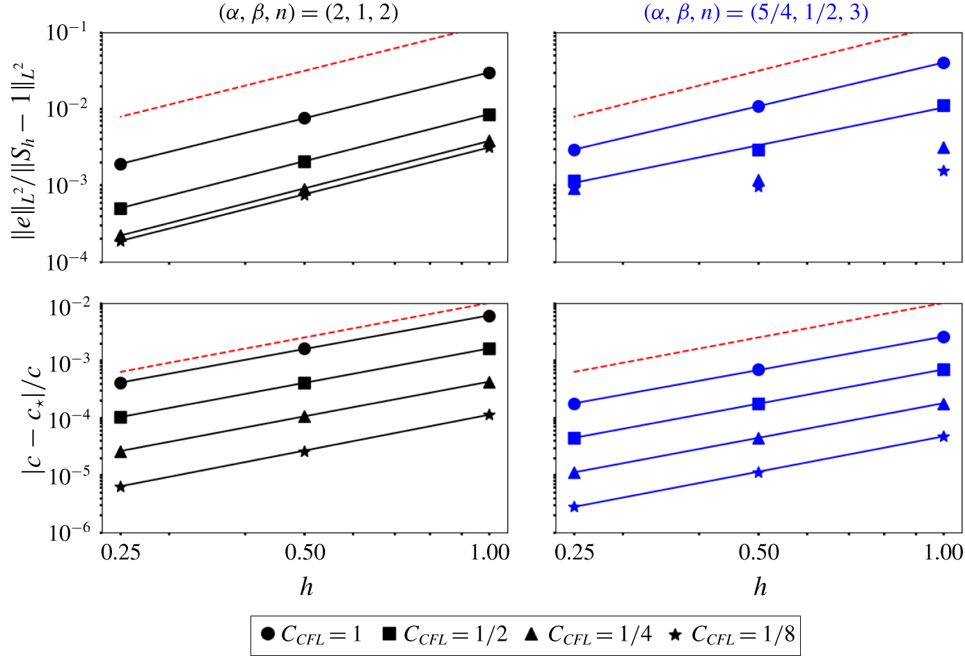
Relative speed and shape errors at time  $T=500$ (laminar) and
 $T=945$ (turbulent) for a range of mesh spacings
 $h$ and CFL numbers
 $C_{CFL}=(c\unicode[STIX]{x1D6FF}t)/h$. The shape error
 $\Vert e\Vert _{L^{2}}$ is defined in figure 9. The parameters chosen are
 $(\unicode[STIX]{x1D6FC},\unicode[STIX]{x1D6FD},n,c)=(2,1,2,{\textstyle \frac{5}{2}})$ for laminar flow and
 $(\unicode[STIX]{x1D6FC},\unicode[STIX]{x1D6FD},n,c)=({\textstyle \frac{5}{4}},{\textstyle \frac{1}{2}},3,1.3223)$ for turbulent flow. The domain length is
 $L=2000$. The red dashed lines denote quadratic convergence in
 $h$. The shape error converges at an approximately quadratic rate as
 $h$ is refined for the laminar flow parameters. The shape error for the turbulent parameters converges at a nearly quadratic rate in
 $h$ for the larger CFL numbers, but stalls for the smaller CFL numbers at small
 $h$. The numerical wave speed
 $c_{\star }$ converges to
 $c$ quadratically as
 $\unicode[STIX]{x0394}t$ and
 $h$ are refined for both laminar and turbulent flow parameters.

Appendix B. Variational formulation
Here we provide a variational characterization of solitary wave solutions to
 $$\begin{eqnarray}\displaystyle & S_{t}+Q_{x}=0, & \displaystyle\end{eqnarray}$$
 $$\begin{eqnarray}\displaystyle & Q=S^{\unicode[STIX]{x1D6FC}}|1+N_{x}|^{\unicode[STIX]{x1D6FD}}\text{sgn}(1+N_{x}), & \displaystyle\end{eqnarray}$$
 $$\begin{eqnarray}\displaystyle & N=-|S^{-1}S_{t}|^{p}\text{sgn}(S_{t}), & \displaystyle\end{eqnarray}$$
where  $p=1/n$ and the subscripts denote differentiation. We seek solutions
 $S(x,t)\equiv S(x-ct)$ to (B 1)–(B 3) that satisfy the conditions at infinity
 $$\begin{eqnarray}\lim _{|x|\rightarrow \infty }S(x,t)=1,\quad \lim _{|x|\rightarrow \infty }S_{x}(x,t)=0.\end{eqnarray}$$
Inserting the ansatz, integrating once and using the conditions in (B 4), we obtain
 $$\begin{eqnarray}c-1-cS+S^{\unicode[STIX]{x1D6FC}}\frac{|1+c^{p}S^{\unicode[STIX]{x1D6FC}}(\text{sgn}(S_{x})|S^{-1}S_{x}|^{p})_{x}|^{\unicode[STIX]{x1D6FD}}}{\text{sgn}(1+c^{p}S^{\unicode[STIX]{x1D6FC}}(\text{sgn}(S_{x})|S^{-1}S_{x}|^{p})_{x})}=0.\end{eqnarray}$$
Rearranging and multiplying by  $S^{-((\unicode[STIX]{x1D6FC}/\unicode[STIX]{x1D6FD})+1)}$ results in
 $$\begin{eqnarray}S^{-1}P(S)-c^{p}S^{-1}(\text{sgn}(S_{x})|S^{-1}S_{x}|^{p})_{x}=0,\end{eqnarray}$$
where  $P$ is defined in (5.6). Equation (B 6) is the Euler–Lagrange equation for the functional
 $$\begin{eqnarray}{\mathcal{E}}[S]=\int _{-\infty }^{+\infty }{\mathcal{I}}_{P}(S)+\frac{c^{p}}{p+1}|S^{-1}S_{x}|^{p+1}\,\text{d}x,\end{eqnarray}$$
where  ${\mathcal{I}}_{P}$ is defined in (5.9). Thus, solitary wave solutions to (B 1)–(B 3) are critical points of the functional
 ${\mathcal{E}}$. The form of
 ${\mathcal{E}}$ mirrors the phase plane energy function
 ${\mathcal{H}}$ (5.8). Numerical tests show that
 ${\mathcal{E}}$ is not time invariant for general solutions of (B 1).