1. Introduction
It is known that the conductive state of a thin liquid film heated from below is subject to two kinds of monotonic Marangoni instability, the short-wave cellular instability (Pearson Reference Pearson1958) and the long-wave deformational instability (Sternling & Scriven Reference Sternling and Scriven1964; Smith Reference Smith1966). The latter type of instability dominates in very thin films or under microgravity conditions.
The manifestations of the Marangoni instabilities in multilayer fluid systems are much more diverse (for a review, see Nepomnyashchy, Simanovskii & Legros (Reference Nepomnyashchy, Simanovskii and Legros2012)). The instabilities can develop for heating both from below and from above, and it can be both monotonic and oscillatory (Nepomnyashchy & Simanovskii Reference Nepomnyashchy and Simanovskii2007).
A specific kind of a multilayer fluid system is a droplet on a liquid substrate (‘liquid lens’). The processes in that system have important applications in engineering, including liquid-phase microextraction (Yamini, Rezazadeh & Seidi Reference Yamini, Rezazadeh and Seidi2019), droplet-based microfluidics (Labanieh et al. Reference Labanieh, Nguyen, Zhao and Kang2015), oil-spill cleanup (Ju et al. Reference Ju, Yang, Li, Cheng and Shi2019), droplet-based floating electrodes (Chen et al. Reference Chen, Zhou, Li, Zhu, Handschuh-Wang, Zhu, Zhou, Liu, Gan and Zhou2018) and DNA studies (Shimazaki et al. Reference Shimazaki, Shiratori, Harada, Nakagawa, Tanaka and Uematsu2021). In some experiments, oscillatory convection flows in a droplet generated by the thermocapillary effect and buoyancy were observed (Rybalko, Magome & Yoshikawa Reference Rybalko, Magome and Yoshikawa2004; Song et al. Reference Song, Moon, Lee, Kim and Pak2014; Buffone Reference Buffone2019). Recently, instabilities of the flow in a floating droplet, similar to those formerly found in a two-layer film, have been revealed by numerical simulations in Nepomnyashchy & Simanovskii (Reference Nepomnyashchy and Simanovskii2021).
In applications, it can be important to control the instability, i.e. to eliminate it or support a definite kind of the flow. The most widespread tool for excitation and suppression of instabilities is vibration (Gershuni & Lyubimov Reference Gershuni and Lyubimov1998). In the case of Marangoni instability caused by heating, the temporal modulation of heating intensity can be a more efficient way for instability excitation and control (Gershuni, Nepomnyashchy & Velarde Reference Gershuni, Nepomnyashchy and Velarde1992; Or & Kelly Reference Or and Kelly2002; Smorodin et al. Reference Smorodin, Mikishev, Nepomnyashchy and Myznikova2009). Specifically, in the case of an oscillatory Marangoni instability, the modulation of the substrate temperature can lead to the parametric excitation of Marangoni waves (Nepomnyashchy & Simanovskii Reference Nepomnyashchy and Simanovskii2015). In the supercritical parameter region, the action of heating modulation on the nonlinear Marangoni wave either creates a two-frequency quasiperiodic motion or leads to frequency locking (Nepomnyashchy & Simanovskii Reference Nepomnyashchy and Simanovskii2020). The influence of a temporal parameter modulation on the droplet instabilities has not yet been studied.
The direct solution of equations governing droplet dynamics is rather difficult, because in addition to the calculation of flow fields, it is necessary to track interfaces and compute the motion of the triple line. For that goal, one applies numerical methods, e.g. the boundary integral method (Manga & Stone Reference Manga and Stone1995), the volume of fluid method (Scardovelli & Zaleski Reference Scardovelli and Zaleski1999) and the level set method (Smith, Ottino & de la Cruz Reference Smith, Ottino and de la Cruz2004). A significant simplification of the mathematical model can be achieved in the case of a slender droplet by means of the long-wave approximation (Oron, Davis & Bankoff Reference Oron, Davis and Bankoff1997). Still, the description of the triple-line motion is technically difficult due to numerous boundary and matching conditions (Kriegsmann & Miksis Reference Kriegsmann and Miksis2003; Huth et al. Reference Huth, Jachalski, Kitavtsev and Peschka2015). Those difficulties can be avoided by means of the precursor model similar to that developed in the case of a droplet on a solid surface (Craster & Matar Reference Craster and Matar2006).
In the present paper, the dynamics of a droplet on a liquid substrate under the action of a temporal cooling modulation on the bottom is investigated. The long-wave approximation and precursor model are applied. We show that the temporal modulation can significantly change the shape of the droplet and lead to the appearance of rhombic droplets.
The structure of the paper is as follows. The formulation of the problem is given in § 2. In § 3, the numerical approach as well as droplet oscillations under the action of temporally modulated heating are described. Section 4 contains concluding remarks.
2. Formulation of the problem
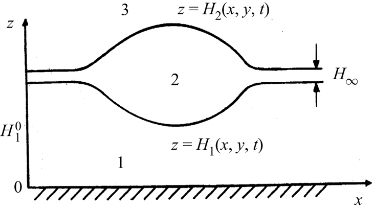
We consider a droplet of liquid 2 that floats on a layer of liquid 1, and it is in contact with the gas phase 3 (see figure 1). The gravity acceleration is  $g$. The
 $m$th fluid has density
 $\rho _m$, dynamic viscosity
 $\eta _m$ and thermal conductivity
 $\kappa _m$. The deformable interfaces are described by equations
 $z=H_1(x,y,t)$ and
 $z=H_2(x,y,t)$.
Geometric configuration of the region and coordinate axes.
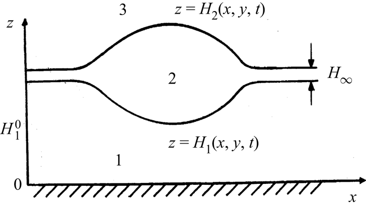
In order to avoid technical difficulties with the description of the triple-line dynamics, we apply the precursor model that presents the droplet and the liquid substrate as a two-layer film.
Following Craster & Matar (Reference Craster and Matar2006), we assume that outside the droplet, liquid 1 is separated from the gas phase by an ultrathin precursor film of liquid 2. The balance between forces on the triple line is achieved by an appropriate choice of the disjoining pressure. Far from the droplet, the equilibrium thickness of layer 1 is  $H_1^{0}$, and the thickness of the precursor film is
 $H_2-H_1=H_{\infty }$ (see figure 1).
Let us emphasize that the precursor model can be applied in different cases. If the spreading coefficient  $S=\sigma _{31}-\sigma _{12}-\sigma _{23}<0$ (partial wetting), using an artificial precursor is just a computational approach. When
 $S>0$ but the Hamaker constant
 $A_2$, which characterizes the interaction of fluids 1 and 3 through the film of fluid 2, is positive, an ultrathin film of fluid 2 is created rather than a macroscopic layer of fluid 2 (pseudopartial wetting). From the macroscopic point of view, both cases are identical.
We do not consider the flow and the heat transfer in the gas. The viscous stresses at the upper boundary are neglected. It is assumed that the temperature of the gas phase is  $T_g$, and the heat exchange coefficient at the liquid–gas interface is
 $q$. The temperature of the solid substrate is
 $T_s(x,y,t)$. The case
 $T_s>T_g$ (
 $T_s< T_g$) corresponds to heating (cooling) the system from the side of the substrate. Below we consider the case of cooling, where the liquid substrate itself is stable, and the instability is caused by the presence of the liquid lens.
Assuming that the temperature differences in the system are not too large, we disregard the dependence of liquid parameters on the temperature, with the following exception. Because the Marangoni convection is caused by the dependence of the interfacial tension coefficients on the temperature, that dependence has to be taken into account. The interfacial tension coefficients on the lower and upper surfaces of the droplets,  $\sigma _1\equiv \sigma _{12}$ and
 $\sigma _2\equiv \sigma _{23}$, are linear functions of temperature
 $T$:
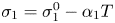 $\sigma _1=\sigma _1^{0}-\alpha _1 T$ and
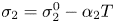 $\sigma _2=\sigma _2^{0}-\alpha _2 T$, where
 $\alpha _1$ and
 $\alpha _2$ are constants.
Later on, we consider a slender droplet, i.e. the slopes of both droplet interfaces are small. Thus, the droplet looks as a thin film of liquid 2 with variable thickness sandwiched between fluids 1 and 3. Therefore, one may expect that the droplet can be subject to long wave instabilities similar to those found in the case of layers. In the present paper, we concentrate on the analysis of that kind of instabilities. In this case, we can apply the mathematical model governing the long-wave dynamics of non-isothermal liquid layers that has been derived using the lubrication approximation in Pototsky et al. (Reference Pototsky, Bestehorn, Merkt and Thiele2005) (see also Nepomnyashchy & Simanovskii Reference Nepomnyashchy and Simanovskii2007, Reference Nepomnyashchy and Simanovskii2010, Reference Nepomnyashchy and Simanovskii2012). Let us note that this approach does not allow us to reveal short-wave instabilities (e.g. a fingering instability of the triple line) characterized by a horizontal scale different from that determined by the droplet size, if any.
In the framework of the long-wave approach, shapes of interfaces  $z=H_1$ and
 $z=H_2$ depend on the scaled horizontal coordinates
 $X=\epsilon x$ and
 $Y=\epsilon y$,
 $\epsilon \ll 1$, rather than on
 $x$ and
 $y$. Also, it is assumed that they depend on the scaled time variable
 $\tau =\epsilon ^{\textbf {2}} t$. A comprehensive description of the long-wave approach can be found in Oron et al. (Reference Oron, Davis and Bankoff1997).
The problem is presented in the non-dimensional form using the equilibrium thickness of the lower layer,  $H_1^{0},$ as the vertical length scale. The choice of the horizontal scale
 $L^{*}$ is arbitrary (Nepomnyashchy & Simanovskii Reference Nepomnyashchy and Simanovskii2012). We choose
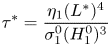 \begin{equation} \tau^{*}=\frac{\eta_1(L^{*})^{4}}{\sigma_1^{0}(H_1^{0})^{3}} \end{equation}
as a time scale and
 \begin{equation} p^{*}=\frac{\sigma_1^{0}H_1^{0}}{(L^{*})^{2}} \end{equation}
as a pressure scale.
The non-dimensional parameters of the problem are defined as follows:
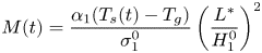 \begin{equation} M(t)=\frac{\alpha_1(T_s (t)-T_g)}{\sigma_1^{0}}\left(\frac{L^{*}}{H_1^{0}}\right)^{2} \end{equation}
is the modified Marangoni number, which is a function of the horizontal coordinates,
 \begin{equation} Bi=\frac{qH_1^{0}}{\kappa_2} \end{equation}
is the Biot number,  $\eta =\eta _1/\eta _2$,
 $\kappa =\kappa _1/\kappa _2$,
 $\sigma =\sigma _2^{0}/\sigma _1^{0}$,
 $\alpha =\alpha _2/\alpha _1$,
 $\rho =\rho _2/\rho _1$ and
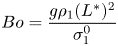 \begin{equation} Bo=\frac{g\rho_1(L^{*})^{2}}{\sigma_1^{0}} \end{equation}
is the Bond number.
In the framework of the lubrication approximation, the velocity and pressure fields are enslaved to the deformations of interfaces. The temporal evolution of those deformations is governed by the volume conservation equations:
 $$\begin{gather} h_{1\tau}+\boldsymbol{\nabla}\boldsymbol{\cdot}\boldsymbol{q}_1=0,\quad h_{2\tau}+ \boldsymbol{\nabla}\boldsymbol{\cdot}\boldsymbol{q}_2=0, \end{gather}$$
 $$\begin{gather}\boldsymbol{q}_1=f_{11}\boldsymbol{\nabla} p_1+f_{12}\boldsymbol{\nabla} p_2+\boldsymbol{q}_1^{\rm T},\quad \boldsymbol{q}_2=f_{21}\boldsymbol{\nabla} p_1+f_{22}\boldsymbol{\nabla} p_2+\boldsymbol{q}_2^{\rm T}. \end{gather}$$
All the quantities in (2.6a,b), (2.7a,b) are non-dimensional;  $h_j=H_j/H_1^{0}$,
 $p_j=P_j/p^{*}$,
 $j=1,2$.
The expressions for mobilities  $f_{ij}$,
 $i,j=1,2$, are
 $$\begin{gather} f_{11}={-}\frac{1}{3}h_1^{3},\quad f_{12}={-}\frac{1}{2}h_1^{2}(h_2-h_1), \end{gather}$$
 $$\begin{gather}f_{21}=\frac{1}{6}h_1^{3}-\frac{1}{2}h_1^{2}h_2,\quad f_{22}= (h_2-h_1)\left[h_1^{2}\left(\frac{1}{2}-\frac{\eta}{3}\right) +h_1h_2\left({-}1+\frac{2\eta}{3}\right)-\frac{\eta}{3}h_2^{2}\right]. \end{gather}$$
The expressions for pressures,
 $$\begin{gather} p_1={-}\nabla^{2}h_1-\sigma\nabla^{2}h_2+Boh_1+Bo\rho(h_2-h_1)+w_1(h_1,h_2), \end{gather}$$
 $$\begin{gather}p_2={-}\sigma\nabla^{2}h_2+Bo\rho h_2+w_2(h_1,h_2), \end{gather}$$
include the contributions of the Laplacian pressures, hydrostatic pressures and disjoining pressures.
Fisher & Golovin (Reference Fisher and Golovin2005) have suggested the following expressions for the disjoining pressures in a two-layer film:
 \begin{equation} w_1=\frac{a_0-a_1-a_2}{h_2^{3}}+\frac{a_1}{h_1^{3}},\quad w_2=\frac{a_0-a_1-a_2}{h_2^{3}}+\frac{a_2}{(h_2-h_1)^{3}}, \end{equation}
where  $a_0$,
 $a_1$ and
 $a_2$ are non-dimensional Hamaker constants. Because the thickness of liquid layer 1 is always macroscopic, we can take
 $w_1=0$. In layer 2, we apply the following expression for the disjoining pressure:
 \begin{equation} w_2=\frac{a}{(h_2-h_1)^{3}}\left[1-\left(\frac{h_{\infty}}{h_2-h_1}\right)^{3}\right], \end{equation}
where  $a$ is the non-dimensional Hamaker constant, which is related to the dimensional Hamaker constant
 $A$ as
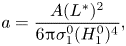 \begin{equation} a=\frac{A(L^{*})^{2}}{6{\rm \pi}\sigma_1^{0}(H_1^{0})^{4}}, \end{equation}
and 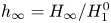 $h_{\infty }=H_{\infty }/H_1^{0}$ (for details, see Craster & Matar (Reference Craster and Matar2006) and Pototsky, Oron & Bestehorn (Reference Pototsky, Oron and Bestehorn2019)).
The non-dimensional expressions for the rates of the thermocapillary flows are
 \begin{align} \boldsymbol{q}_1^{\rm T}&={-}\frac{h_1^{2}}{2}\boldsymbol{\nabla}\{M[1+d(\alpha\kappa-Bi h_1\}, \end{align}
 \begin{align} \boldsymbol{q}_2^{\rm T} &={-}\frac{\eta\alpha\kappa}{2}h_2^{2}\boldsymbol{\nabla} (Md) \nonumber\\ &\quad +\frac{(2h_2-h_1)h_1}{2}\boldsymbol{\nabla}\{M[{-}1+Bi h_1d-\alpha\kappa(1-\eta)d]\}, \end{align}
where
 \begin{equation} d=[\kappa+Bi(1-\kappa)h_1+Bi\kappa h_2]^{{-}1}. \end{equation}
3. Nonlinear simulations
3.1. Numerical approach
In the present section, we describe the results of numerical simulations performed in the framework of system (2.6a,b)–(2.16). The evolution equations were discretized by central differences for spatial derivatives and solved using an explicit scheme. In the framework of this scheme, the fields on the next time step have been calculated through the corresponding fields on the previous time step. The convergence of that approach with the decrease of the mesh size was formerly studied by Nepomnyashchy & Simanovskii (Reference Nepomnyashchy and Simanovskii2015). Periodic boundary conditions have been applied on the boundaries of the computational region  $L \times L$,
 $L=240$. Periodic boundary conditions correspond to an infinite system of droplets moving synchronously.
Recall that in the present paper we assume that the characteristic horizontal scale of the surface deformations is significantly larger than the thicknesses of the droplet and the substrate layer. The computations have been performed in the computational region, using a grid of  $80\times 80$.
Actually, the fields  $h_1$ and
 $h_2$ are rather smooth; thus the
 $80\times 80$ grid gives a good resolution of large-scale wave patterns. The choice of parameters in the present paper has been done after some trial simulations on
 $100\times 100$ and
 $120\times 120$ grids.
Some additional convergence tests on  $60\times 60$,
 $80\times 80$ and
 $100\times 100$ grids can be found in figure 4 of Nepomnyashchy & Simanovskii (Reference Nepomnyashchy and Simanovskii2015), and no qualitative changes have been observed.
The simulations have been carried out during at least  $10^{6}$ non-dimensional time units. In all the simulations, the change of the fields
 $h_m$,
 $m=1,2$, was less than
 $0.3\,\%$. The time step typically changed between 0.00125 and 0.005, which is significantly below the linear scheme stability boundary. No quantitative changes have been observed for simulations made with different time steps.
We used two kinds of initial conditions. First, we applied the initial conditions
 \begin{equation} h_1(X,Y,0)=1;\quad h_2(X,Y,0)=h_-{+}h_+\exp\{-[(X-L/2)^{2}+(Y-L/2)^{2}]/R^{2}\}, \end{equation}
i.e. a droplet of liquid 2 with a Gaussian shape was imposed on a flat layer of liquid 1. In some other simulations, we used the shape of the droplet obtained in the previous simulations carried out for a different set of parameters as the initial condition, and continued simulations for the new set of parameters.
The system under consideration is characterized by five non-dimensional parameters that correspond to the ratios of physical parameters and three other parameters that describe the external actions on the system (non-dimensional temperature difference, heat transfer on the liquid–gas interface and gravity). It looks impossible to analyse the influence of all those parameters. Therefore, we restrict ourselves to the investigation of a particular system of liquids, as is usually done in the case of multilayer systems.
In the present paper, we perform computations for the system of fluorinert FC70 (liquid 1) and silicone oil 10 (liquid 2). This system of liquids was used in microgravity experiments (see, e.g. Géoris et al. Reference Géoris, Hennenberg, Lebon and Legros1999). We applied the following set of liquid parameters that was formerly used in simulations of Marangoni instability in two-layer systems (Nepomnyashchy & Simanovskii Reference Nepomnyashchy and Simanovskii2012):  $\eta =3.04$,
 $\kappa =0.522$,
 $\alpha =2$,
 $\rho =0.482$,
 $\sigma =2.6$.
 $h_-=1.02$,
 $h_+=1$,
 $R=60$,
 $h_{\infty }=0.01$,
 $Bo=0$ and
 $Bi=20$. The value of
 $a_2$ is chosen equal to
 $3\times 10^{-6}$ (see Nepomnyashchy & Simanovskii Reference Nepomnyashchy and Simanovskii2021).
Note that in the absence of gravity, a liquid layer with a deformable interface is subject to a monotonic Marangoni instability for arbitrary small  $M>0$, i.e. for arbitrary weak heating from below (Sternling & Scriven Reference Sternling and Scriven1964). That instability is not saturable, and it leads to the rupture of the substrate layer. The temperature disturbance caused by the droplet acts as a ‘seed’ of instability. Therefore, in the presence of the temperature gradient, one can expect the existence of a stable configuration containing a droplet on a layer flat on the infinity only if
 $M<0$, i.e. by cooling from below.
3.2. Nonlinear regimes in the absence of modulation
In the present subsection, we describe briefly some results of numerical simulations carried out for  $M={\rm const.}$ (for details, see Nepomnyashchy & Simanovskii (Reference Nepomnyashchy and Simanovskii2021)).
It is known that in the absence of gravity and the thermocapillary effect ( $M=Bo=0$), both interfaces of an equilibrium droplet are spherical caps. The exact formulas that follow from the balance of interfacial tensions on the triple line are given, for example, by Princen (Reference Princen1969). In the long-wave limit, these interfaces become paraboloids:
 \begin{equation} h_1=1+a(r^{2}-r_0^{2}),\quad h_2=1-\frac{a}{\sigma}(r^{2}-r_0^{2});\quad r< r_0, \end{equation}
where  $r$ is the radial coordinate,
 $a$ is a constant and
 $r_0$ is the droplet's radius. The paraboloidal surface profiles satisfy (2.6a,b)–(2.11). They correspond to constant pressures in the droplet and in the substrate and to zero flow rates.
For moderate values of  $|M|$ the droplet is stationary and axisymmetric. The isolines
 $h_1(X,Y)$ and
 $h_2(X,Y)$ are perfectly circular. However, the shapes of the interfaces change drastically. While in the case
 $M=0$ the second derivatives
 ${{\rm d}}^{2}h_1/{{\rm d}}r^{2}$ and
 ${{\rm d}}^{2}h_2/{{\rm d}}r^{2}$ are of different signs, at
 $M<0$ they are typically of the same sign, at least for sufficiently large
 $Bi|M|$. Indeed, in the latter case the terms
 $\boldsymbol {q}_1^{\rm T}$ and
 $\boldsymbol {q}_2^{\rm T}$ prevail in expression (2.7a,b). At large
 $Bi|M|$, the leading-order terms in expressions (2.15) and (2.16) are proportional to
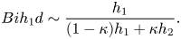 \begin{equation} Bih_1d\sim\frac{h_1}{(1-\kappa)h_1+\kappa h_2}. \end{equation}
Therefore, the flow rates vanish when  $h_1/h_2={\rm const}$. In other words, the lower surface of the droplet
 $z=h_1(r)$ is adjusted to its upper surface
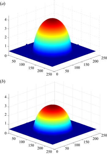
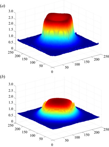
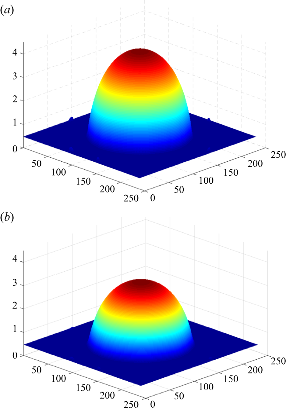
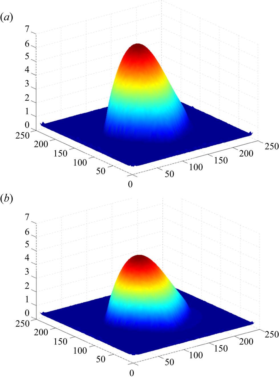
 $z=h_2(r)$ in such a way that the temperature at the interface between the droplet and the substrate is nearly constant, so that the thermocapillary stress that creates thermocapillary flows is diminished. Let us emphasize that although the interfaces of the droplet and the substrate are motionless, there are thermocapillary flows in both the droplet and the substrate. The stresses created by those flows determine the shapes of the droplet surfaces, which are close to parabolic ones (see figure 2).
The stationary shapes of (a) interface  $h_2(X,Y)$ and (b) interface
 $h_1(X,Y)$ for
 $M=-2$,
 $Bo=0$,
 $Bi=20$,
 $\tau =10^{6}$.
With an increase of cooling from below or heating from above, the droplet becomes oscillatory unstable.
The long-wave oscillatory instability of this type was formerly found in a system of two flat liquid layers (Nepomnyashchy & Simanovskii Reference Nepomnyashchy and Simanovskii2007). Because we consider here only the long-wave instability of a flat droplet, we expect that the physical origin of the droplet's instability is essentially the same as in the case of layers, i.e. it is caused by the interaction between deformations of both interfaces mediated by the thermocapillary flow, which is generated by those deformations. Qualitatively, by heating from above, Newton's law at the upper droplet surface creates a certain kind of negative feedback, which in the case of two interfaces can lead to an ‘overstability’, i.e. an oscillatory instability. Note that oscillatory Marangoni instabilities by heating from above have been observed also in some other problems (see Nepomnyashchy et al. Reference Nepomnyashchy, Simanovskii and Legros2012).
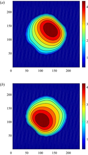
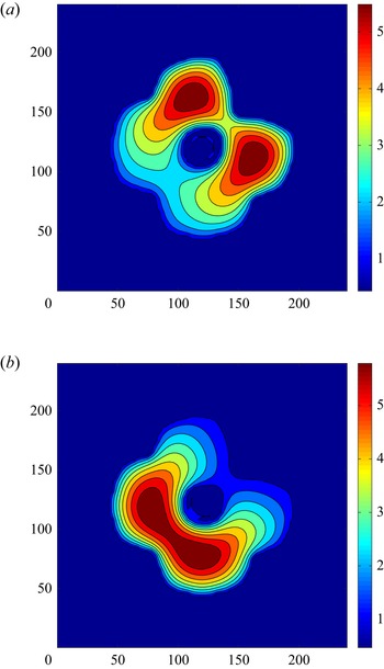
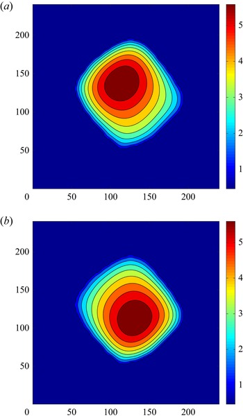
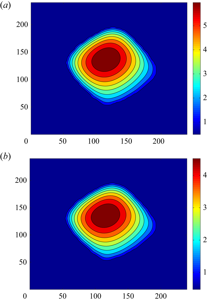
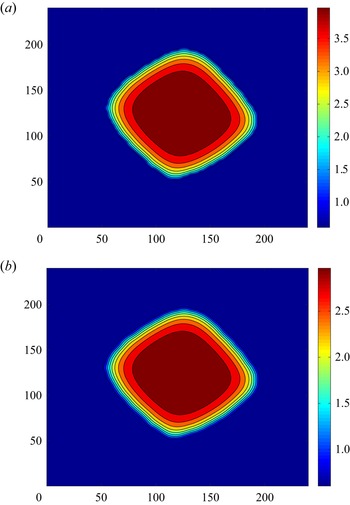
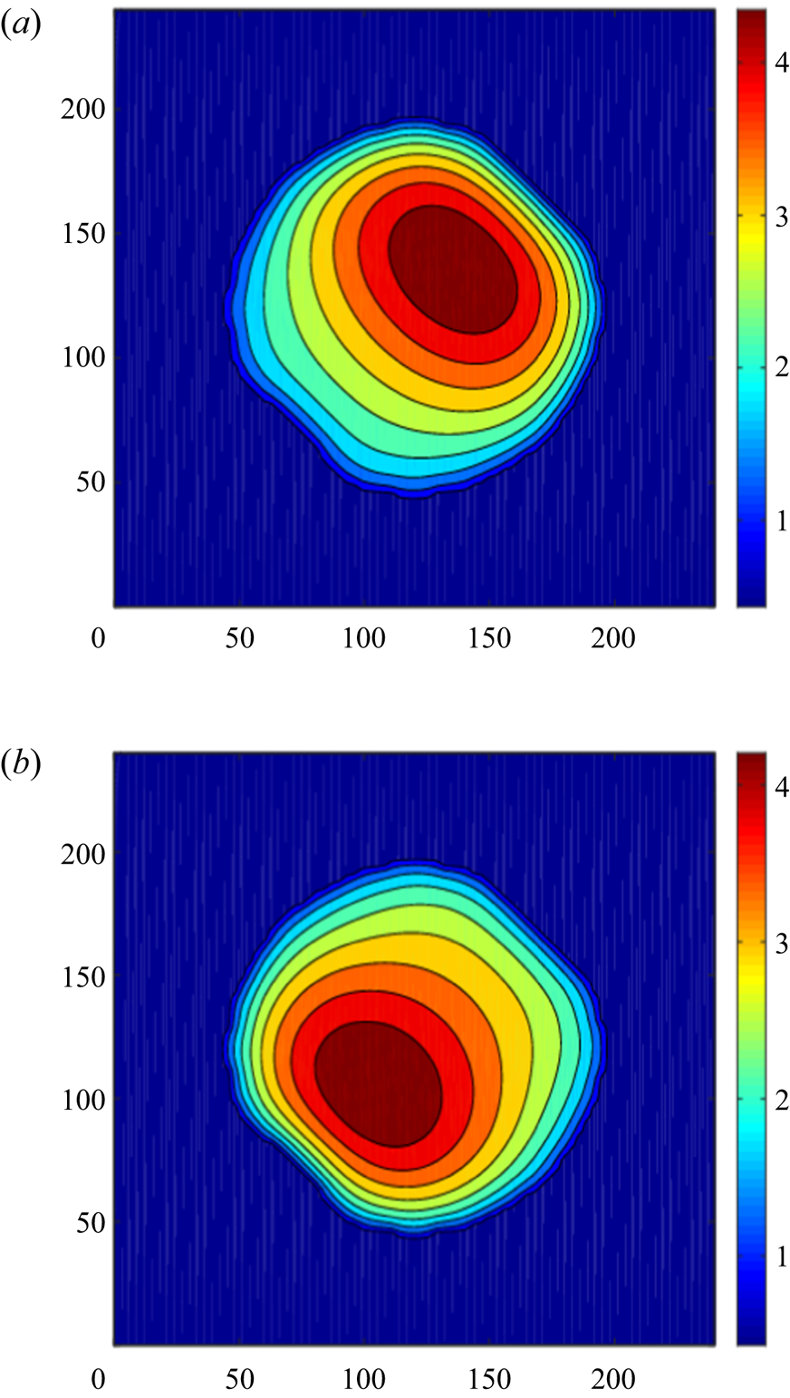
At  $M\leq -2.25$ we observe periodic oscillations characterized by the violation of the rotational symmetry, which corresponds to the azimuthal wavenumber
 $m=1$ (see figure 3). The oscillations are characterized by the symmetry
 \begin{equation} h_m(X,Y,\tau+T/2)=h_m(L-Y,L-X,\tau),\quad m=1,2, \end{equation}
where  $T$ is the period of oscillations. In other words, after a half-period, the shape of the droplet is reflected with respect to the axis
 $X+Y=L$. Therefore, the quantities
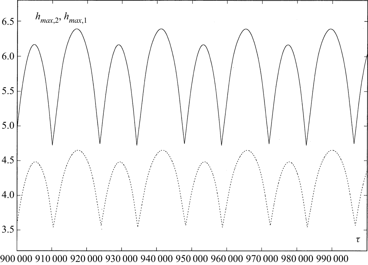
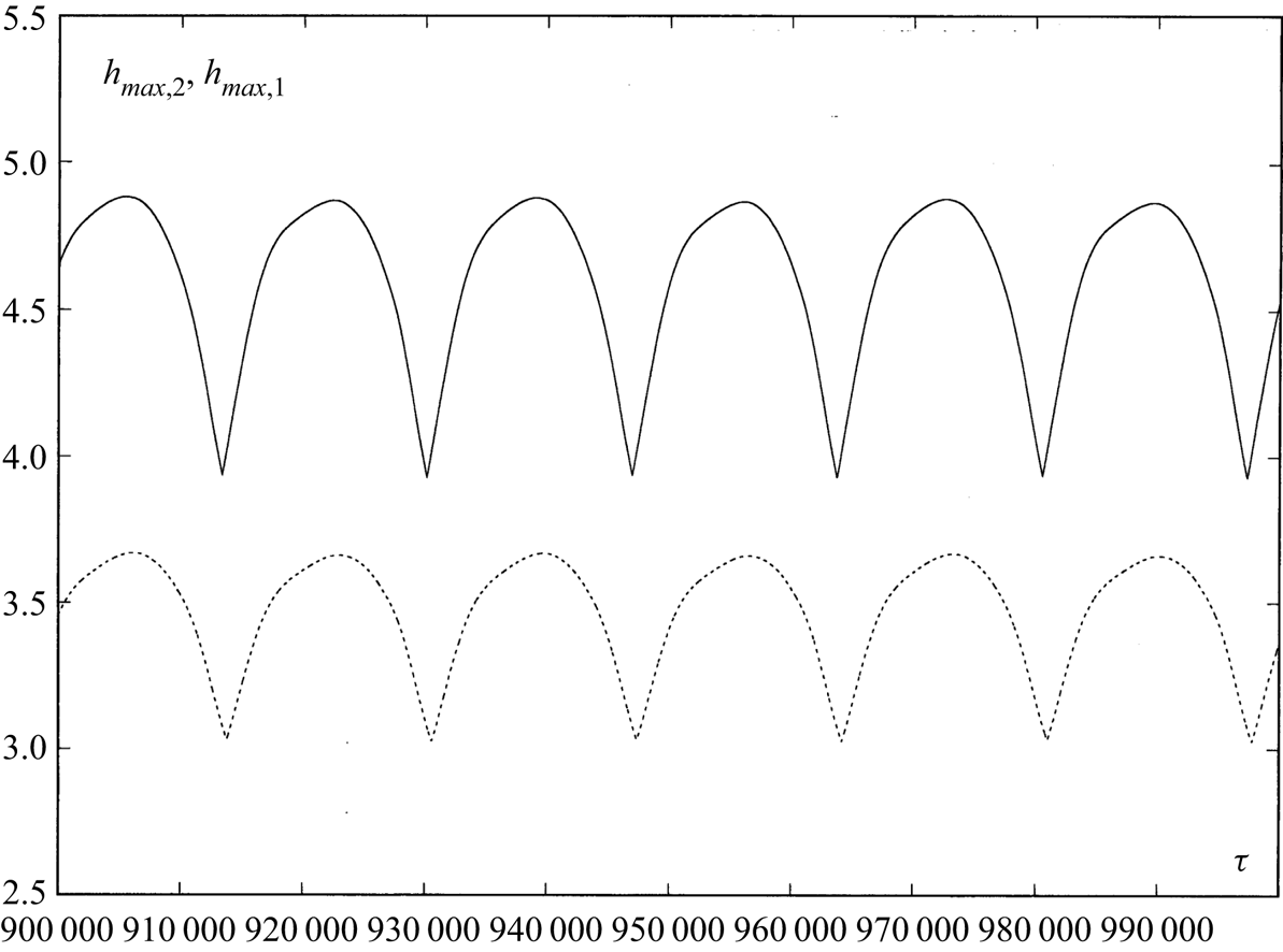
 $h_{max,m}(\tau )=\max h_m(X,Y,\tau )$ and
 $h_{min,m}(\tau )=\min h_m(X,Y,\tau )$ are periodic in time with period
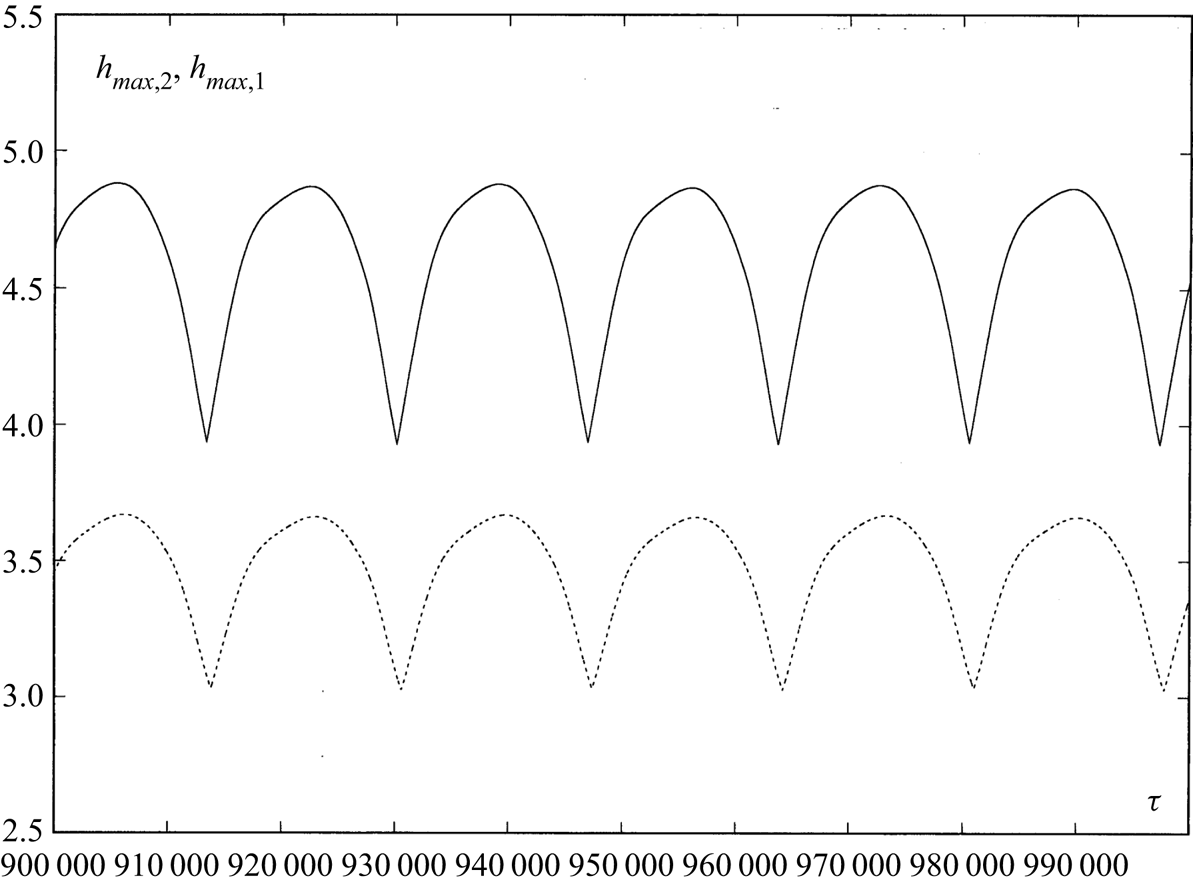
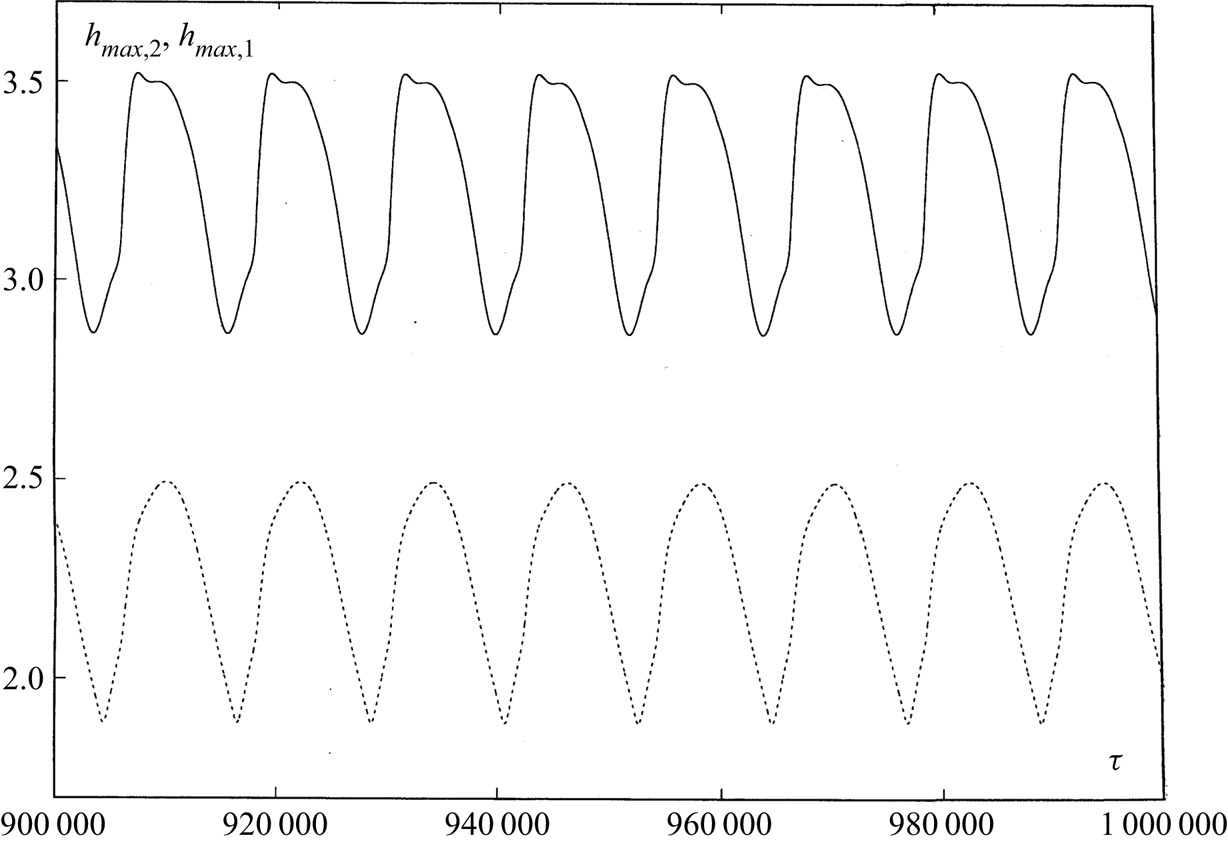
 $T/2$. The temporal evolution of
 $h_{max,1}$ and
 $h_{max,2}$ is shown in figure 4. The type of oscillations described above is observed up to
 $|M|=2.75$.
A snapshot of the fields of  $h_2(X,Y,\tau )$ at (a)
 $\tau =7\times 10^{5}$ and (b)
 $\tau =7.15\times 10^{5}$ for
 $M=-2.5$,
 $Bo=0$,
 $Bi=20$.
The oscillations of  $h_{max,2}(\tau )$ (solid line) and
 $h_{max,1}(\tau )$ (dashed line) for
 $M=-2.5$,
 $Bo=0$,
 $Bi=20$.
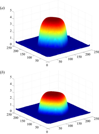
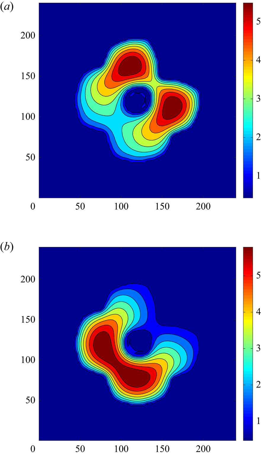
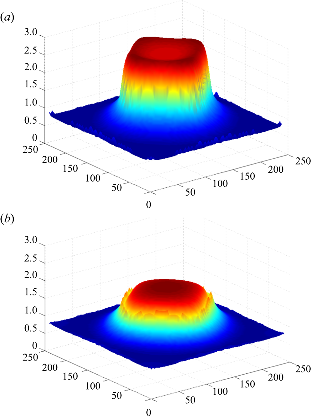
At higher values of  $|M|$, the intensive Marangoni convection leads to a significant change of the droplet shape: a trough near the centre of the droplet is developed and the components with
 $m=3$ and
 $m=4$ become visible (see figure 5). Let us note that the structures presented in figure 5 have also been obtained on
 $100\times 100$ and
 $120\times 120$ grids. The spatial symmetry with respect to the axis
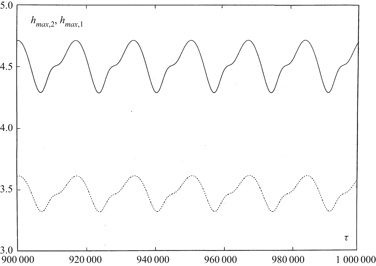
 $X=Y$ is retained, but the symmetry of oscillations (3.4) is violated; therefore the oscillation period of
 $h_{max,m}$ and
 $h_{min,m}$ becomes equal to the full period
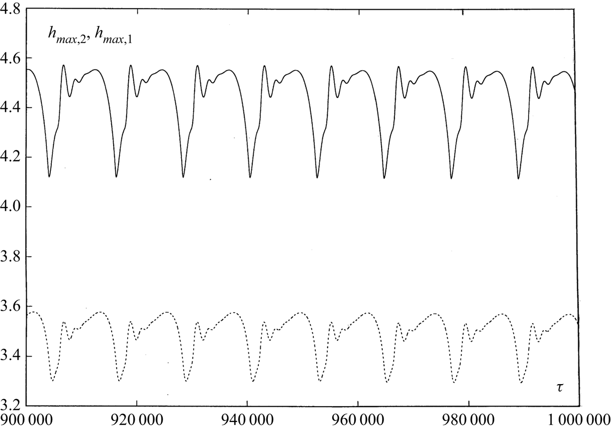
 $T$. The temporal evolution of
 $h_{max,1}$ and
 $h_{max,2}$ is shown in figure 6.
A snapshot of the fields of  $h_2(X,Y,\tau )$ at (a)
 $\tau =6.9\times 10^{5}$ and (b)
 $\tau =7\times 10^{5}$ for
 $M=-4$,
 $Bo=0$,
 $Bi=20$.
The oscillations of  $h_{max,2}(\tau )$ (solid line) and
 $h_{max,1}(\tau )$ (dashed line) for
 $M=-4$,
 $Bo=0$,
 $Bi=20$.
3.3. Time-periodic oscillations
We apply time-periodic modulation of the Marangoni number  $M$, determined by the formula
 \begin{equation} M(\tau)=\bar{M}(1+A\sin\omega\tau),\quad \omega=2{\rm \pi}/T, \end{equation}
where  $A$ is the amplitude and
 $\omega$ is the frequency of modulation.
First, we explore the influence of heating modulation (3.5) on a stationary droplet of liquid 2 on a layer of liquid 1.
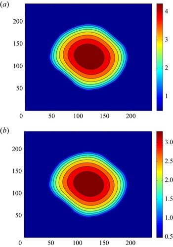
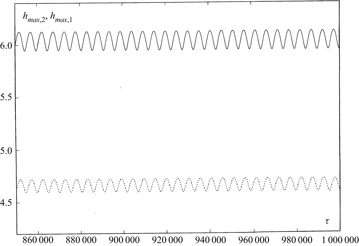
Let us take the round stationary droplet shown in figure 2 as initial condition and consider its evolution under the action of temporal modulation with  $\bar {M}=-2.5$ and
 $\omega =0.000375$. The oscillations of
 $h_{max,m}(\tau )$,
 $m=1,2$, of the initially round droplet are shown in figure 7 and a snapshot of the fields of
 $h_2(X,Y,\tau )$ and
 $h_1(X,Y,\tau )$ is presented in figure 8.
The oscillations of  $h_{max,2}(\tau )$ (solid line) and
 $h_{max,1}(\tau )$ (dashed line) for
 $\bar {M}=-2.5$,
 $Bo=0$,
 $Bi=20$,
 $A=0.25$,
 $\omega =0.000375$.
A snapshot of the fields of (a)  $h_2(X,Y,\tau )$ and (b)
 $h_1(X,Y,\tau )$ for
 $\bar {M}=-2.5$,
 $Bo=0$,
 $Bi=20$,
 $A=0.25$,
 $\omega =0.000375$,
 $\tau =1\times 10^{6}$.
One can see that the shape of oscillations created by heating modulation with  $\bar {M}=-2.5$ is quite different from those generated by the internal instability of the thermocapillary flow at
 $M=-2.5$ (compare figures 7 and 4; 8 and 3). The basic effect is a change of the droplet's shape.
If we use as initial conditions the periodic oscillations of the droplet shown in figure 8 and switch off modulation putting  $A=0$, we get a steady non-round droplet similar to those presented in figure 8. As found in Nepomnyashchy & Simanovskii (Reference Nepomnyashchy and Simanovskii2021), the threshold of the appearance of spontaneous droplet oscillations depends on the shape of the droplet. For a round droplet, the threshold value of oscillatory instability is
 $|M_c|\approx 2.25<2.5$, while for the steady droplet,
 $|M_c|>2.5$. That is why we observe periodic oscillations with the period of the external heating modulation, rather than a superposition of oscillations with two different frequencies, external and internal ones.
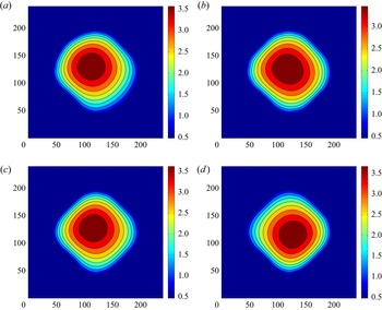
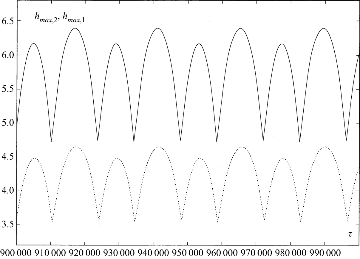
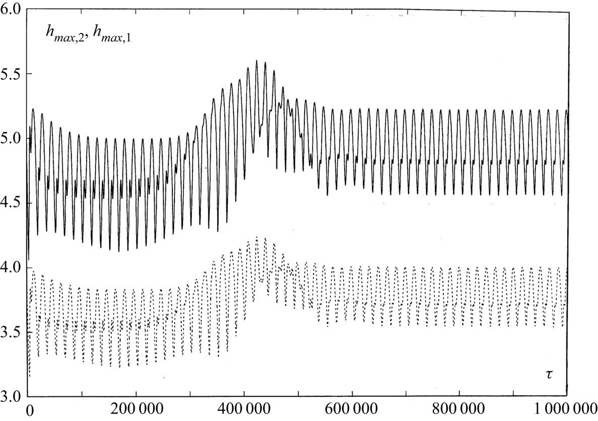
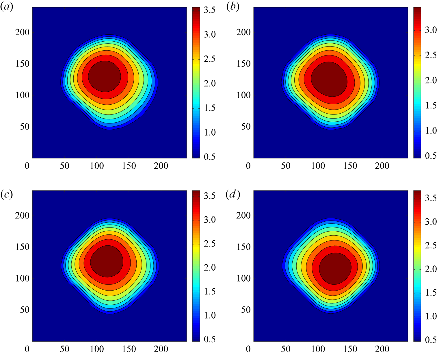
If we use initial conditions corresponding to figure 8 and increase the amplitude of modulation taking  $A=0.5$, we get a further change of the droplet's shape: the droplet becomes ‘rhombic’. The transient process of the change of oscillations and the evolution of the droplet's shape are shown in figures 9 and 10.
The oscillations of  $h_{max,2}(\tau )$ (solid line) and
 $h_{max,1}(\tau )$ (dashed line) for
 $\bar {M}=-2.5$,
 $Bo=0$,
 $Bi=20$,
 $A=0.5$,
 $\omega =0.000375$; as initial conditions we use the structure shown in figure 10.
The fields of  $h_2(X,Y,\tau )$ for
 $\bar {M}=-2.5$,
 $Bo=0$,
 $Bi=20$,
 $A=0.5$,
 $\omega =0.000375$: (a)
 $\tau =100$; (b)
 $\tau =1000$; (c)
 $\tau =4000$; (d)
 $\tau =10\,000$.
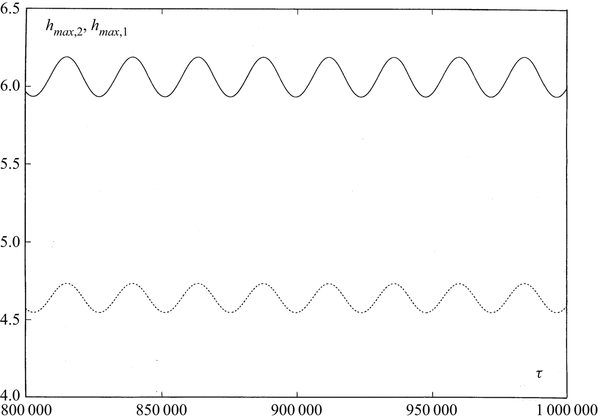
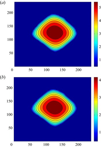
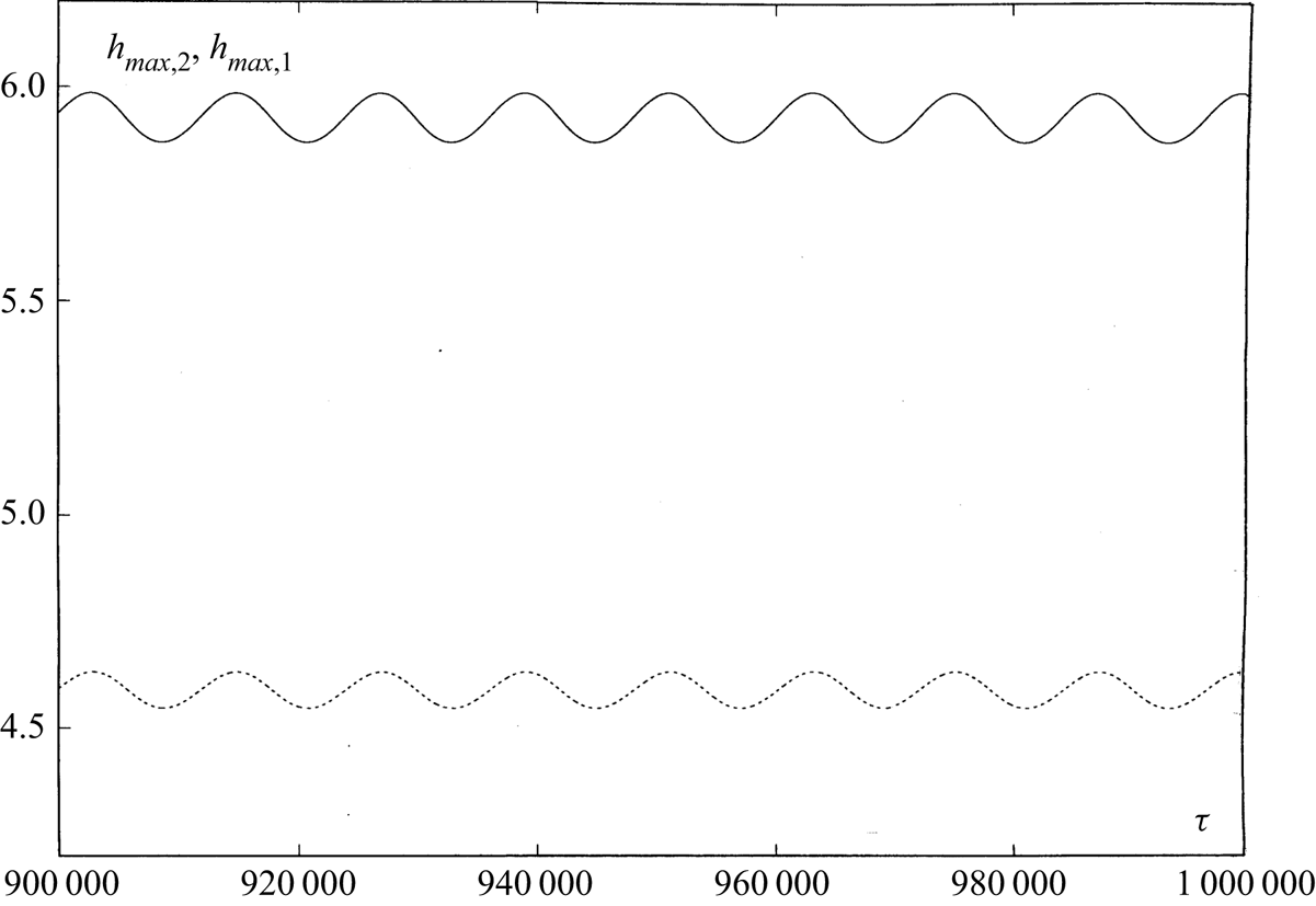
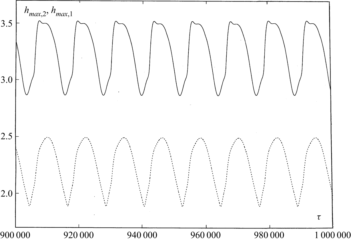
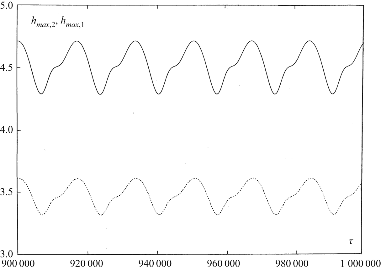
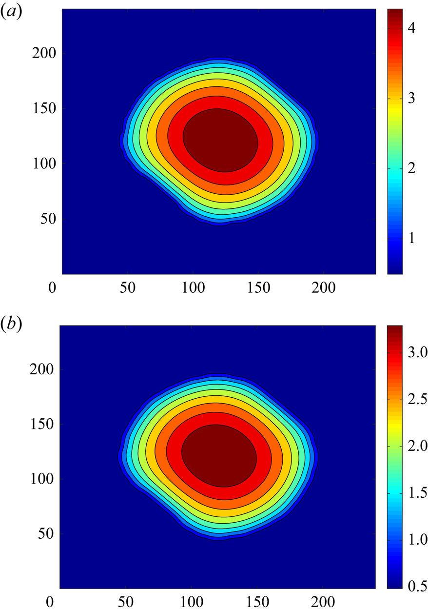
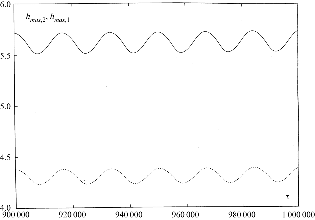
With a decrease of the amplitude of modulation (we take  $A=0.25$), the periodic oscillations of the rhombic droplet become of a rather simple form (see figure 11). A snapshot of the fields of
 $h_2(X,Y,\tau )$ and
 $h_1(X,Y,\tau )$ is shown in figure 12. Thus, for the same values of parameters (
 $\bar {M}=-2.5$,
 $Bo=0$,
 $Bi=20$,
 $A=0.25$ and
 $\omega =0.000375$), we get droplets of different shape from different initial conditions. The characteristics of oscillations are strongly influenced by the droplet's shape. Indeed, the response of the system to an external perturbation depends on the set of eigenfrequencies and eigenfunctions of own droplet oscillations, which is determined by the droplet's shape.
The oscillations of  $h_{max,2}(\tau )$ (solid line) and
 $h_{max,1}(\tau )$ (dashed line) for
 $\bar {M}=-2.5$,
 $Bo=0$,
 $Bi=20$,
 $A=0.25$,
 $\omega =0.000375$.
A snapshot of the fields of (a)  $h_2(X,Y,\tau )$ and (b)
 $h_1(X,Y,\tau )$ for
 $\bar {M}=-2.5$,
 $Bo=0$,
 $Bi=20$,
 $A=0.25$,
 $\omega =0.000375$,
 $\tau =1\times 10^{6}$.
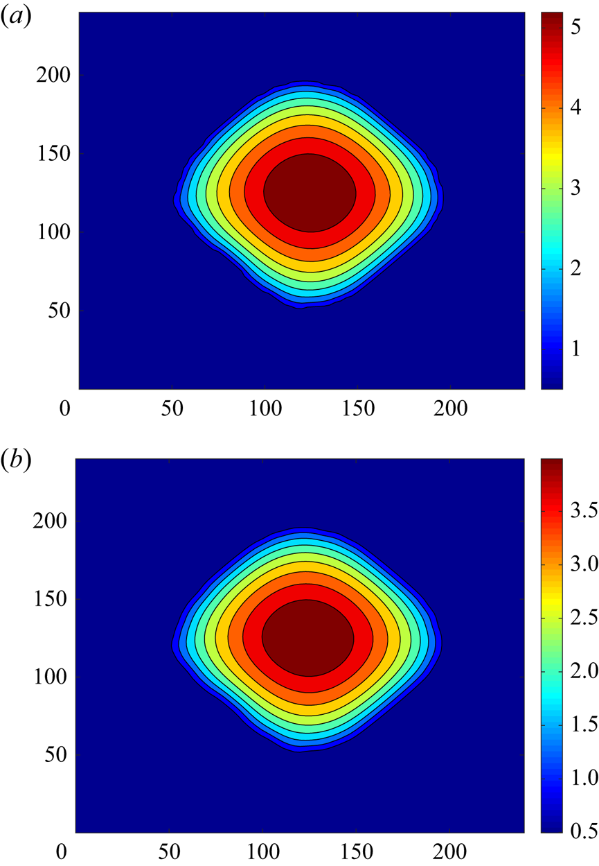
If we use as initial conditions the periodic oscillations of the rhombic droplet (see figure 12) and switch off modulation, i.e. take  $A=0$, we get a steady rhombic droplet similar to those presented in figure 12. Therefore, there is no competition of frequencies. The rhombic droplet oscillates exactly with the imposed period of oscillations whatever it is. Note that in the case
 $M=-2.5$ and
 $A=0$, we get tristability: (i) periodic oscillations of the round droplet obtained in the absence of modulation and two different shapes of a steady droplet, namely (ii) steady round droplet and (iii) steady rhombic droplet.
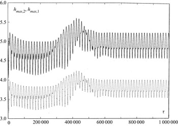
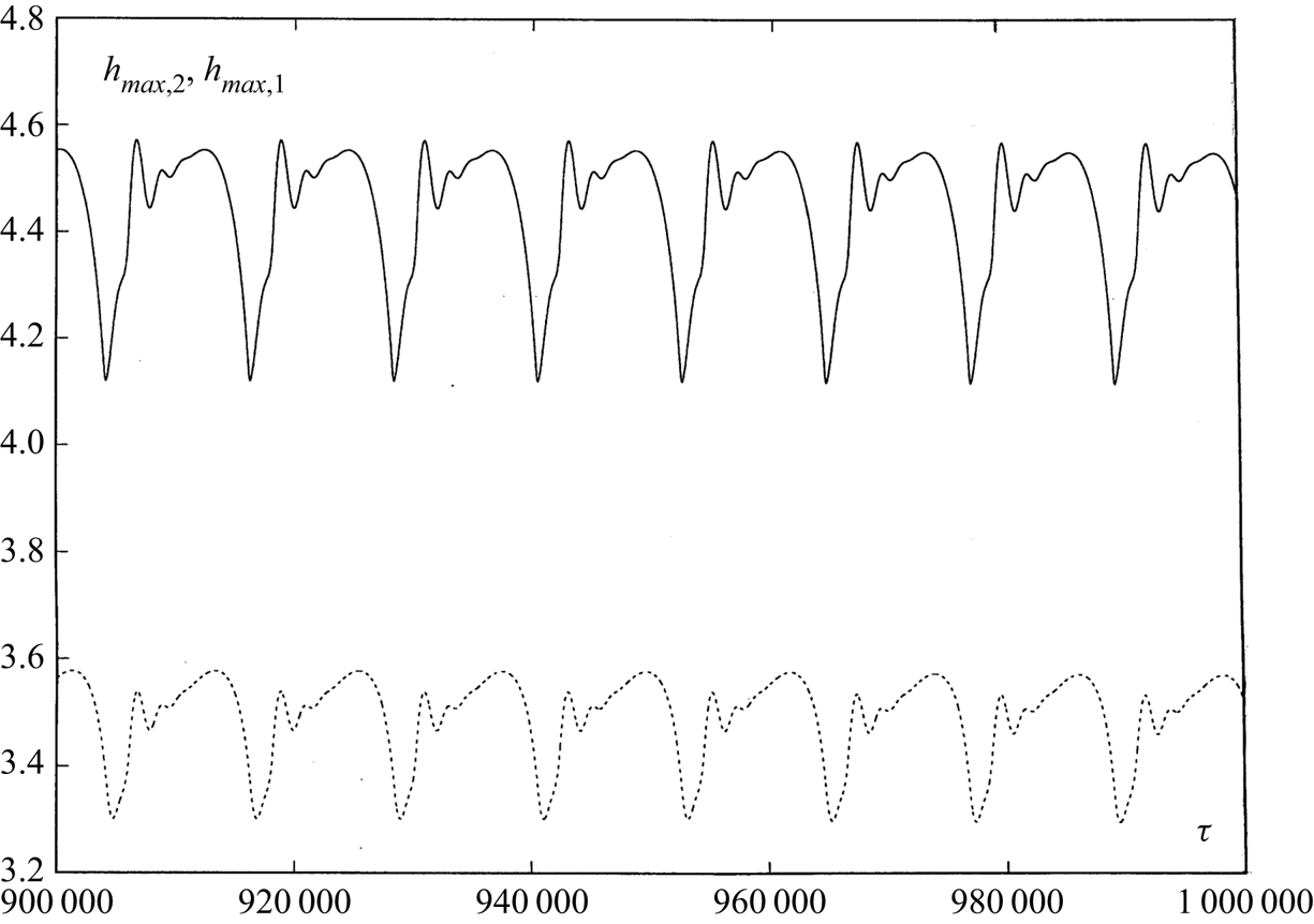
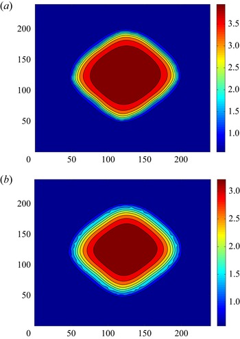
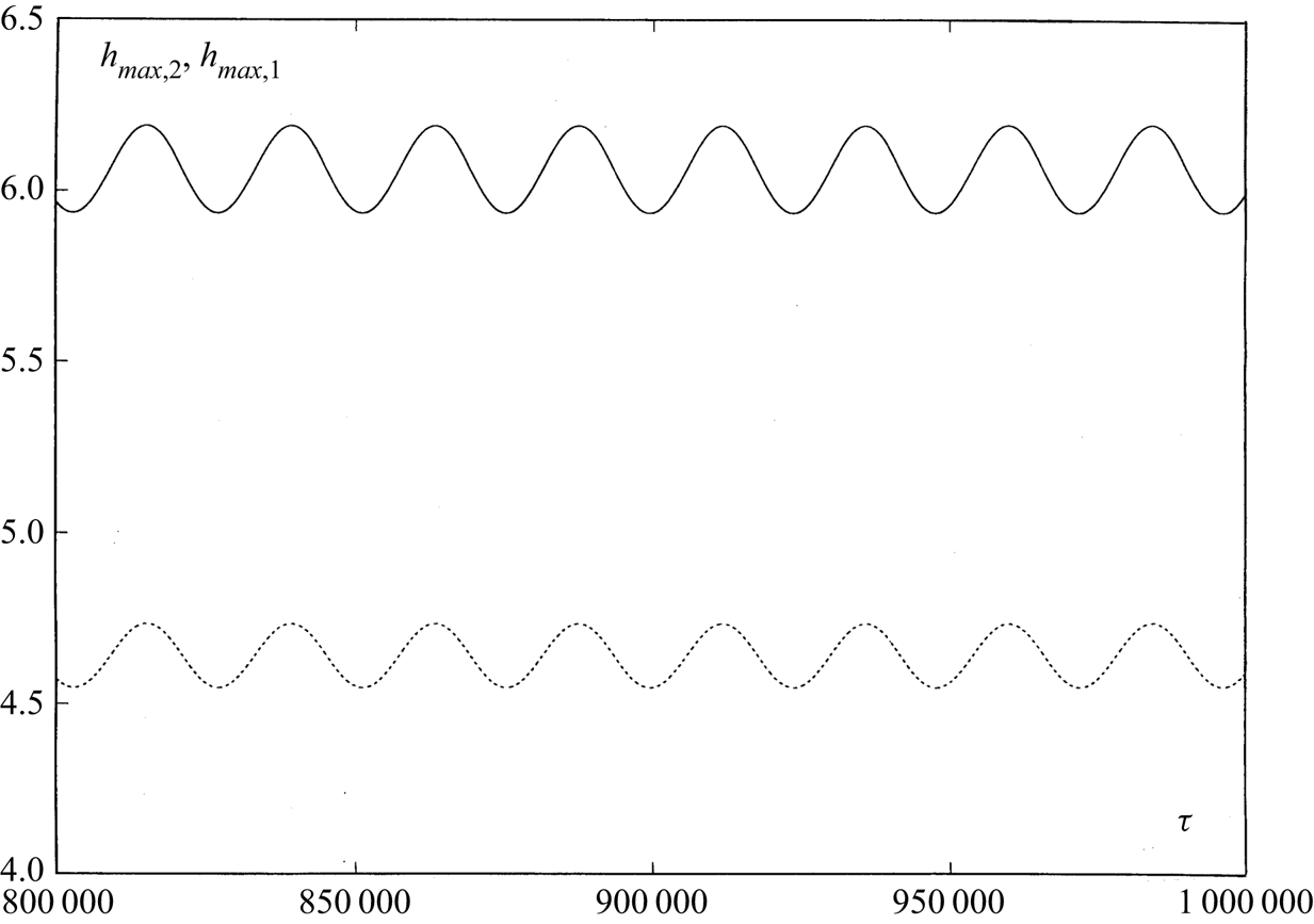
Now, let us increase cooling from below. For  $M=-4$, the round droplet oscillates even without modulation – it has its own frequency (see figures 5 and 6). When we add modulation with another frequency, generally we can get oscillations with two different frequencies. However, if we impose a heating modulation with the ‘main frequency’
 $\omega =0.00026$ close to the frequency of spontaneous oscillations, we observe periodic oscillations of a rhombic droplet shown in figure 13. A snapshot of the fields of
 $h_2(X,Y,\tau )$ and
 $h_1(X,Y,\tau )$ is presented in figure 14.
The oscillations of  $h_{max,2}(\tau )$ (solid line) and
 $h_{max,1}(\tau )$ (dashed line) for
 $\bar {M}=-4$,
 $Bo=0$,
 $Bi=20$,
 $A=0.25$,
 $\omega =0.00026$.
A snapshot of the fields of (a)  $h_2(X,Y,\tau )$ and (b)
 $h_1(X,Y,\tau )$ for
 $\bar {M}=-4$,
 $Bo=0$,
 $Bi=20$,
 $A=0.25$,
 $\omega =0.00026$,
 $\tau =1\times 10^{6}$.
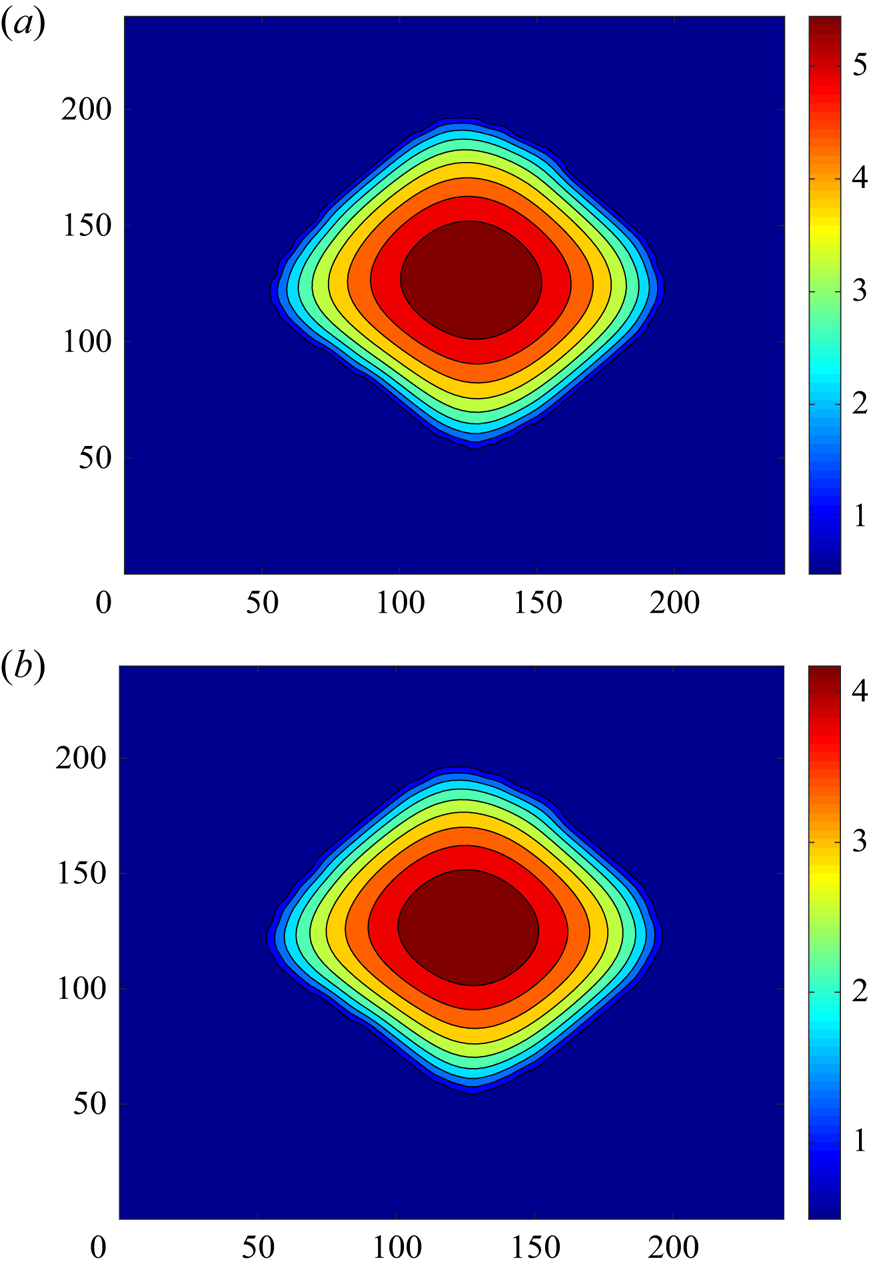
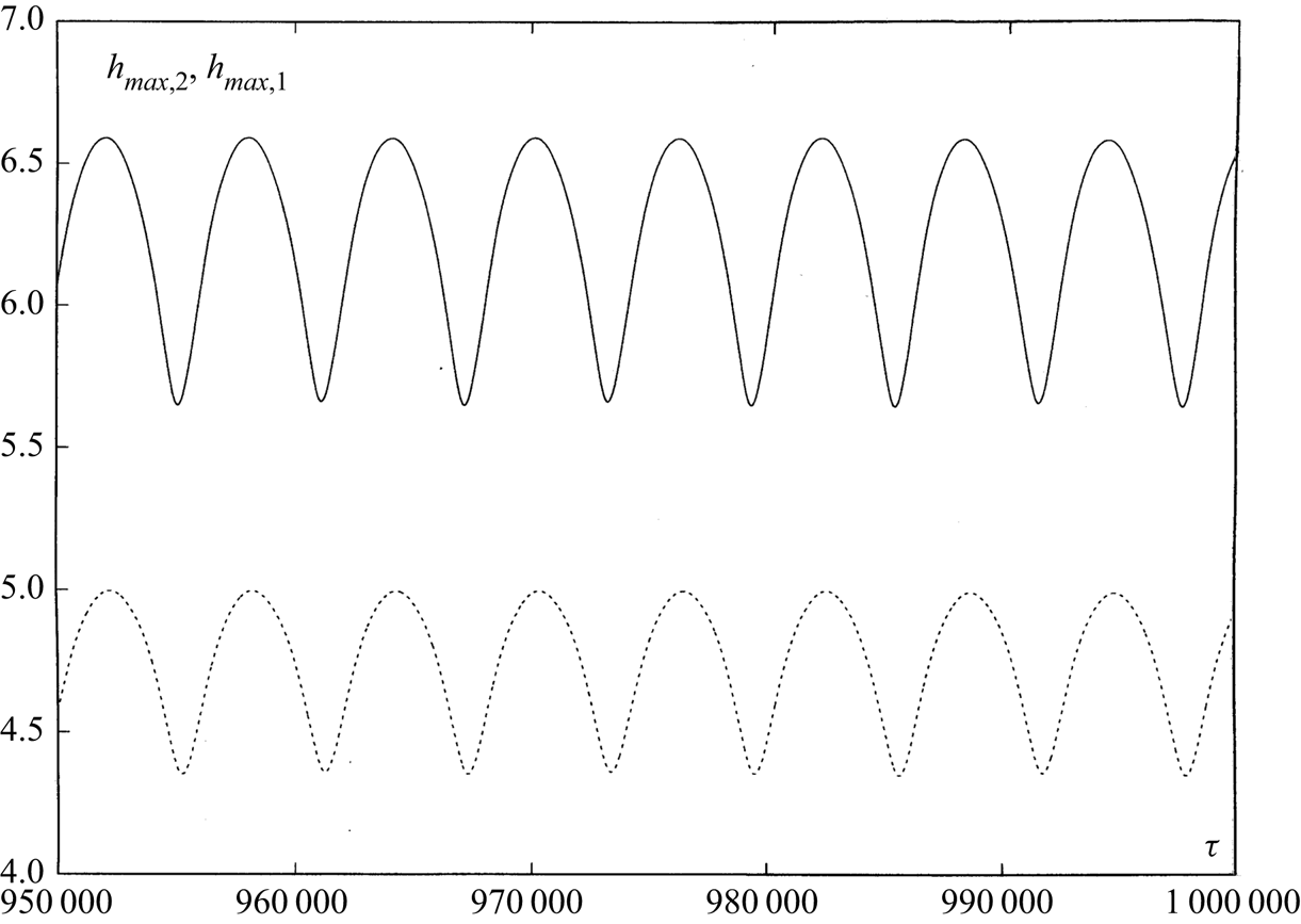
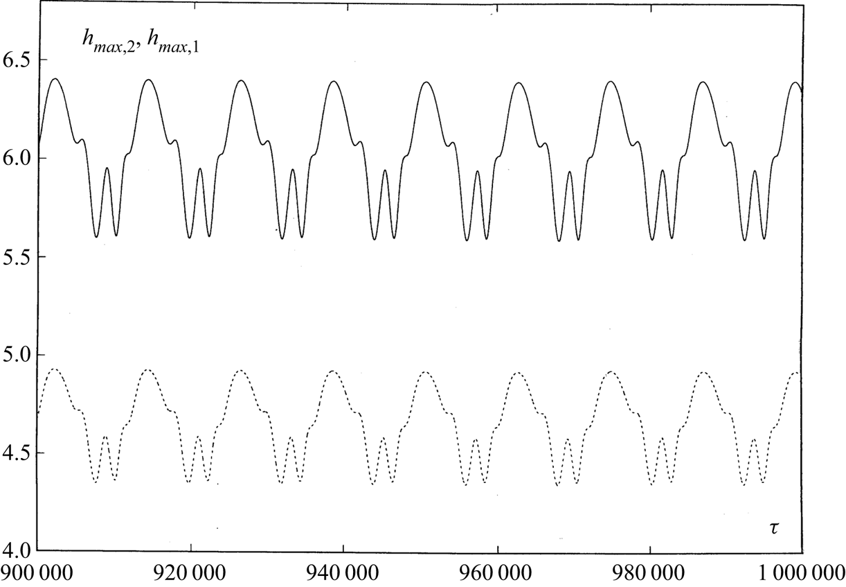
Periodic oscillations of the rhombic droplet with different amplitudes of modulation have been obtained also for the frequency  $\omega _{1} =2 \omega$. Oscillations of
 $h_{max,m}(\tau )$,
 $m=1,2$, for
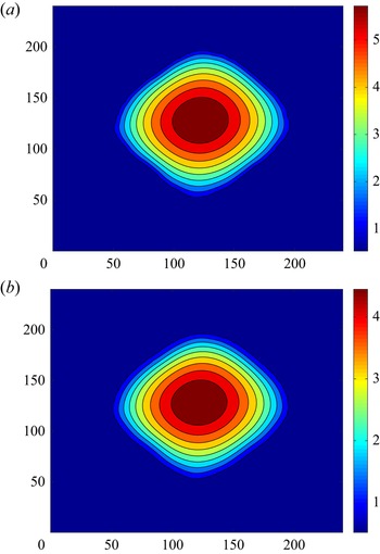
 $A=0.75$ are shown in figure 15 and a snapshot of the fields of
 $h_2(X,Y,\tau )$ and
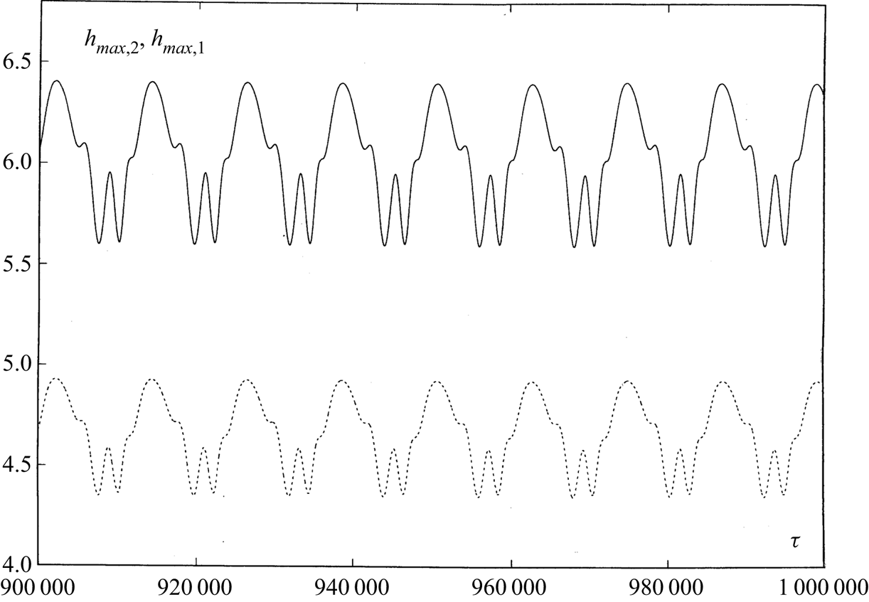
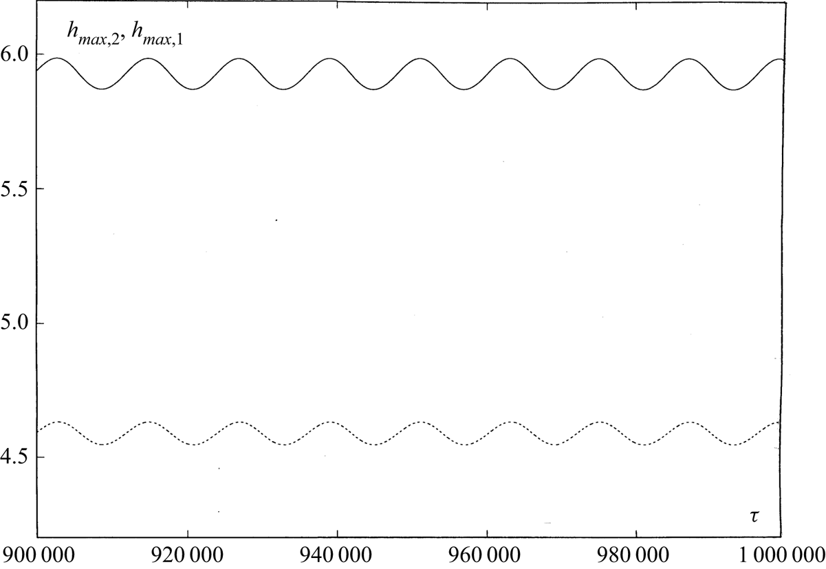
 $h_1(X,Y,\tau )$ is presented in figure 16. With a decrease of the amplitude of modulation, oscillations of
 $h_{max,m}(\tau )$,
 $m=1,2$, are simplified (see figure 17).
The oscillations of  $h_{max,2}(\tau )$ (solid line) and
 $h_{max,1}(\tau )$ (dashed line) for
 $\bar {M}=-4$,
 $Bo=0$,
 $Bi=20$,
 $A=0.75$,
 $\omega =0.00052$.
A snapshot of the fields of (a)  $h_2(X,Y,\tau )$ and (b)
 $h_1(X,Y,\tau )$ for
 $\bar {M}=-4$,
 $Bo=0$,
 $Bi=20$,
 $A=0.75$,
 $\omega =0.00052$,
 $\tau =1\times 10^{6}$.
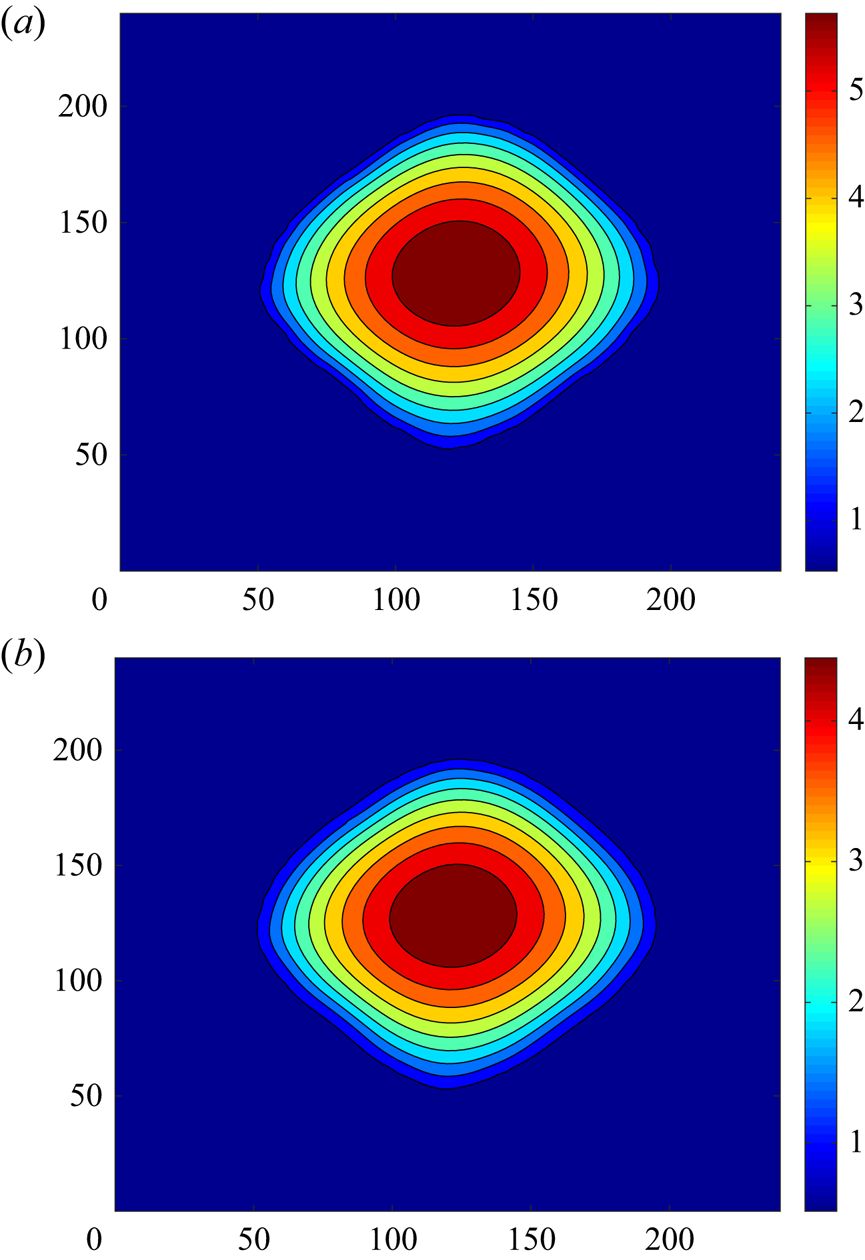
The oscillations of  $h_{max,2}(\tau )$ (solid line) and
 $h_{max,1}(\tau )$ (dashed line) for
 $\bar {M}=-4$,
 $Bo=0$,
 $Bi=20$,
 $A=0.1$,
 $\omega =0.00052$.
3.4. Non-periodic versus periodic oscillations
Now, let us consider temporal modulation for  $\bar {M}=-4$ with the frequency
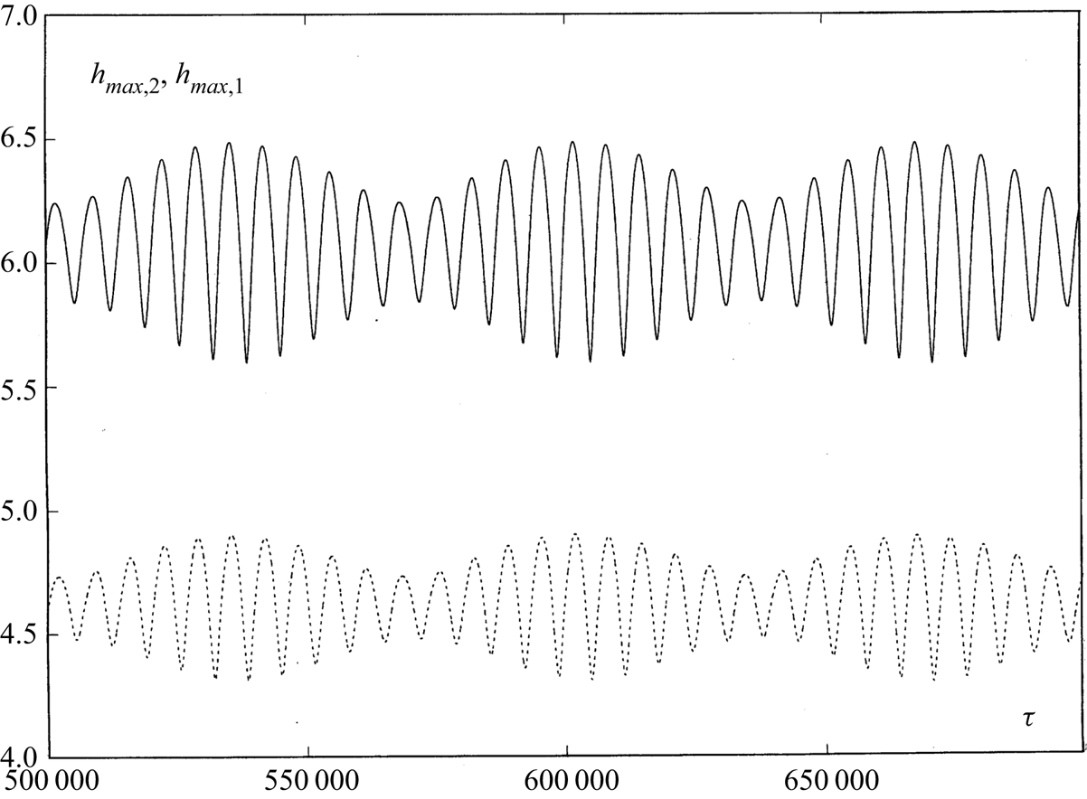
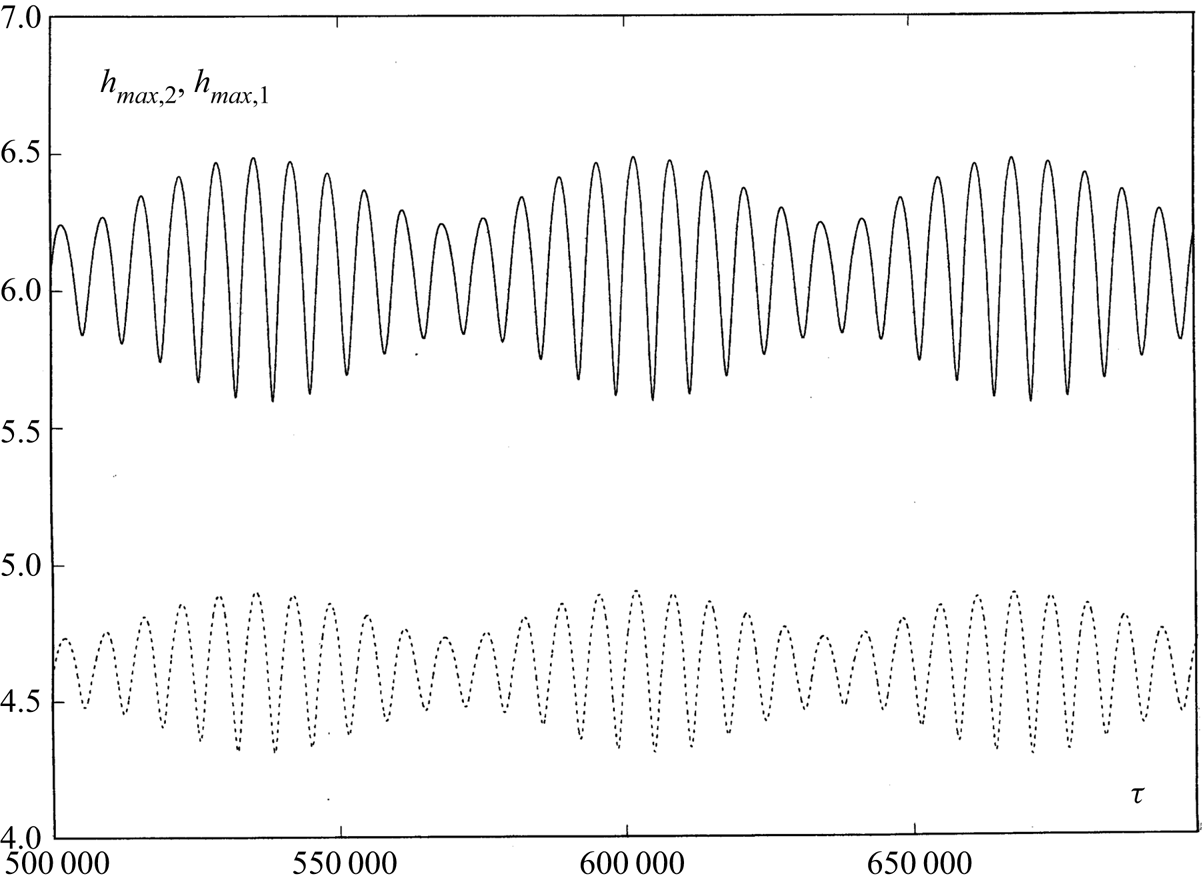
 $\omega _{2}=4 \omega$. In that case, we do not observe a synchronization of internal oscillations to the external modulation, and the motion is quasiperiodic. An example of the quasiperiodic oscillations of
 $h_2(X,Y,\tau )$ and
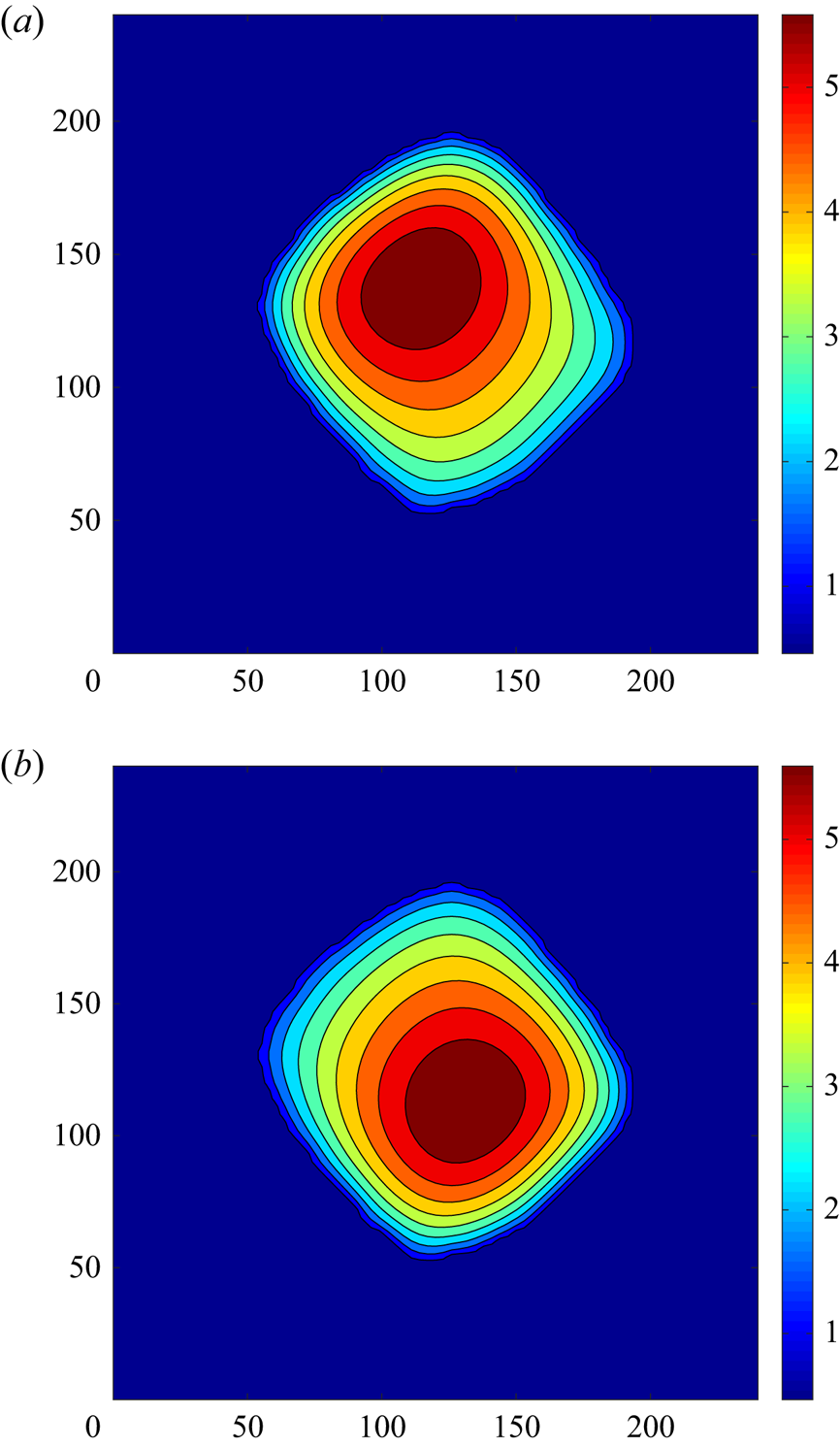
 $h_1(X,Y,\tau )$ is presented in figure 18. Snapshots of the fields of
 $h_2(X,Y,\tau )$ at different instants of time are shown in figure 19. Note that observed oscillations of the rhombic droplet take place along the other diagonal of the computational region than those shown in figure 5.
The oscillations of  $h_{max,2}(\tau )$ (solid line) and
 $h_{max,1}(\tau )$ (dashed line) for
 $\bar {M}=-4$,
 $Bo=0$,
 $Bi=20$,
 $A=0.1$,
 $\omega =0.00104$.
A snapshot of the fields of  $h_2(X,Y,\tau )$ at (a)
 $\tau =540\,000$ and (b)
 $\tau =560\,000$ for
 $\bar {M}=-4$,
 $Bo=0$,
 $Bi=20$,
 $A=0.1$,
 $\omega =0.00104$.
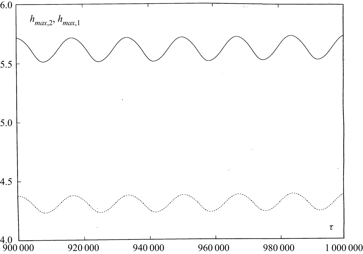
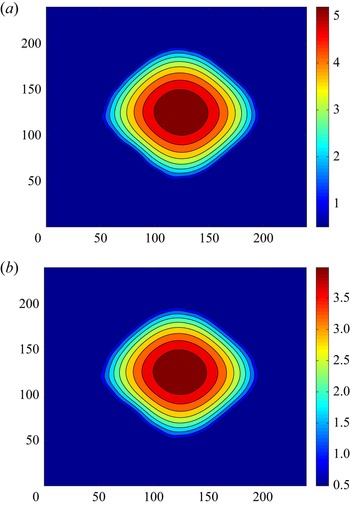
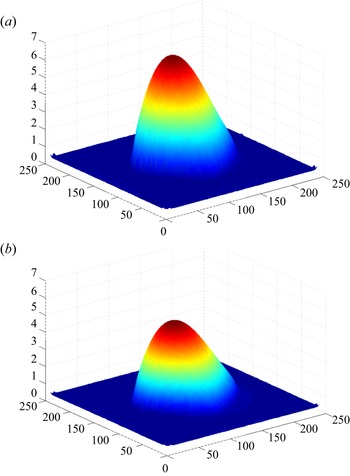
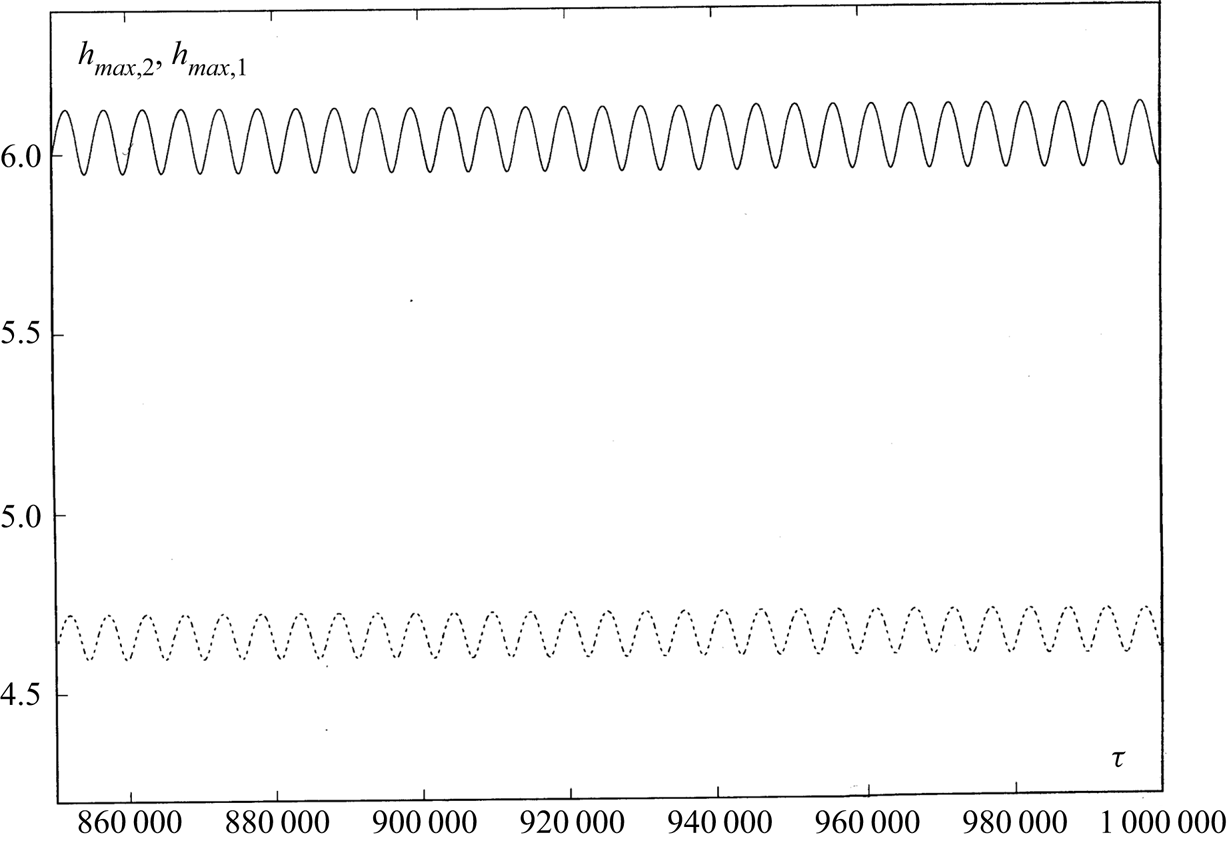
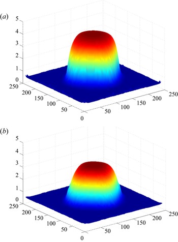
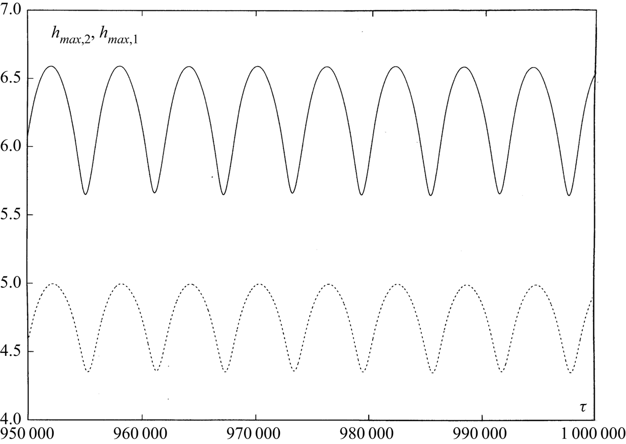
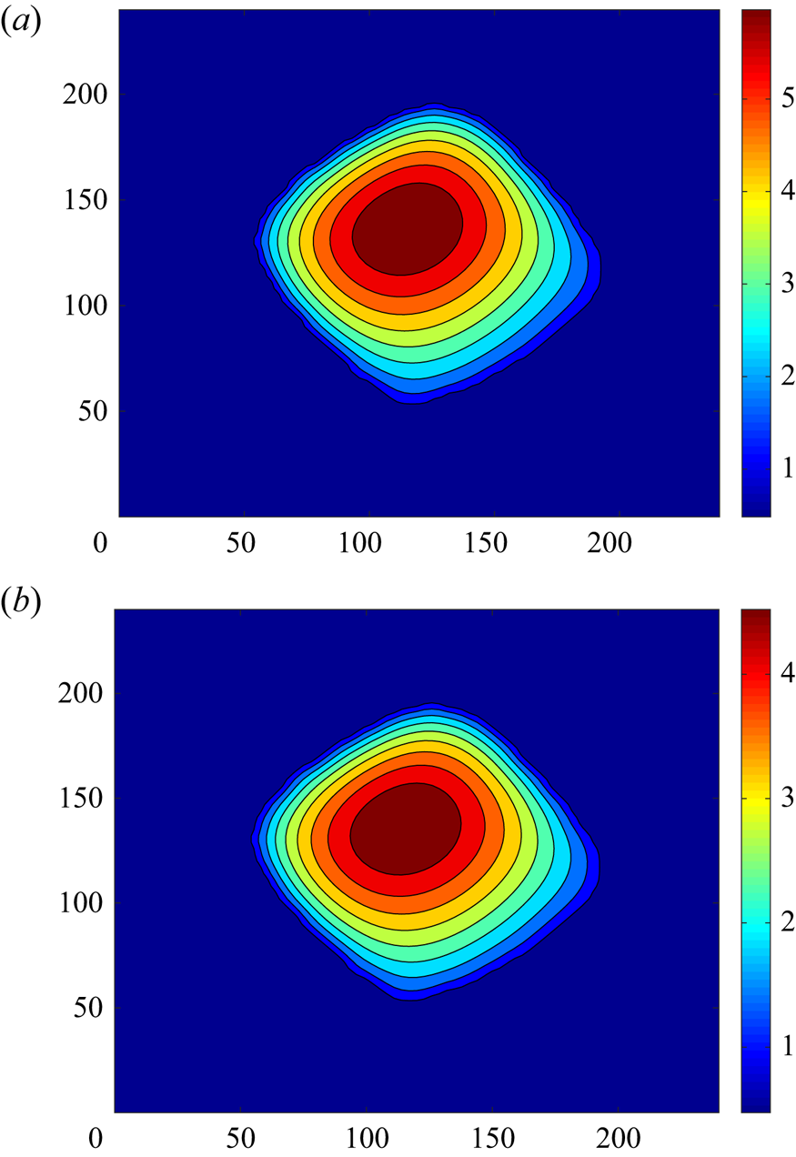
With an increase of the amplitude, the modulation frequency ‘wins’ and we get periodic oscillations of the rhombic droplet (see figure 20). A snapshot of the fields of  $h_2(X,Y,\tau )$ and
 $h_1(X,Y,\tau )$ is shown in figure 21 and the shapes of interfaces are presented in figure 22. The periodic oscillations of the rhombic droplet on
 $\omega _{2} = 4 \omega$ have been also obtained for larger values of the amplitude of modulation (
 $A=0.5$ and
 $A=0.75$; see figure 24).
The oscillations of  $h_{max,2}(\tau )$ (solid line) and
 $h_{max,1}(\tau )$ (dashed line) for
 $\bar {M}=-4$,
 $Bo=0$,
 $Bi=20$,
 $A=0.25$,
 $\omega =0.00104$.
A snapshot of the fields of (a)  $h_2(X,Y,\tau )$ and (b)
 $h_1(X,Y,\tau )$ for
 $\bar {M}=-4$,
 $Bo=0$,
 $Bi=20$,
 $A=0.25$,
 $\omega =0.00104$,
 $\tau =1\times 10^{6}$.
The shapes of (a) interface  $h_2(X,Y,\tau )$ and (b) interface
 $h_1(X,Y,\tau )$ for
 $\bar {M}=-4$,
 $Bo=0$,
 $Bi=20$,
 $A=0.25$,
 $\omega =0.00104$,
 $\tau =1\times 10^{6}$.
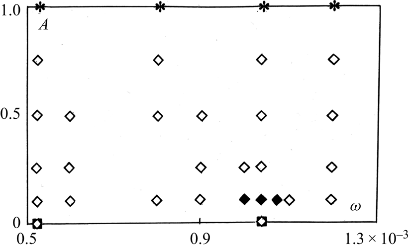
If we take as initial conditions the snapshot corresponding to quasiperiodic oscillations presented in figure 18 and increase the frequency (we take  $\omega =0.0012$), the modulation frequency wins and we get periodic oscillations of the rhombic droplet shown in figure 23. The diagram of regimes in the plane
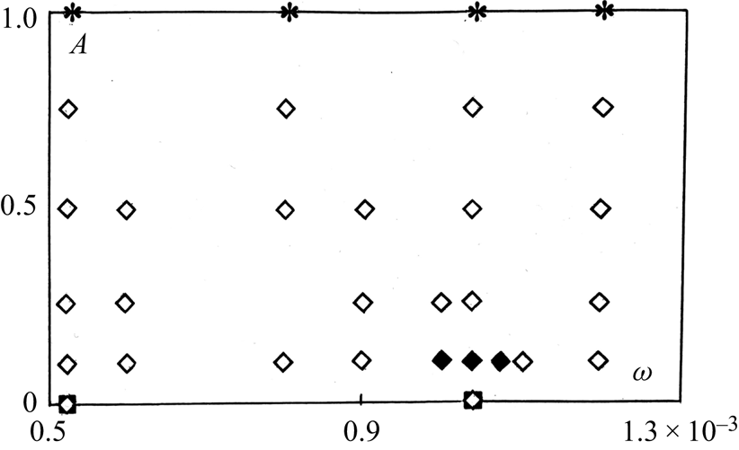
 $(\omega, A)$ is constructed in figure 24.
The oscillations of  $h_{max,2}(\tau )$ (solid line) and
 $h_{max,1}(\tau )$ (dashed line) for
 $\bar {M}=-4$,
 $Bo=0$,
 $Bi=20$,
 $A=0.1$,
 $\omega =0.0012$.
The diagram of flow regimes in the plane  $(\omega, A)$ for
 $M=-4$,
 $Bo=0$,
 $Bi=20$. White diamonds, periodic oscillations; black diamonds, beatings; black squares, steady states; asterisks, irregular oscillations.
3.5. The influence of gravity on droplet dynamics
Now, let us consider the action of gravity on the droplets. If we take the rhombic droplet shown in figure 16 as the initial condition (frequency  $\omega _{1} =2 \omega$), under the action of gravity (
 $Bo=0.05$) the amplitude of periodic oscillations decreases (cf. figures 25 and 15) and the droplet is essentially flattened. A snapshot of the fields of
 $h_2(X,Y,\tau )$ and
 $h_1(X,Y,\tau )$ is shown in figure 26 and the shapes of interfaces are presented in figure 27.
The oscillations of  $h_{max,2}(\tau )$ (solid line) and
 $h_{max,1}(\tau )$ (dashed line) for
 $\bar {M}=-4$,
 $Bo=0.05$,
 $Bi=20$,
 $A=0.75$,
 $\omega =0.00052$.
A snapshot of the fields of (a)  $h_2(X,Y,\tau )$ and (b)
 $h_1(X,Y,\tau )$ for
 $\bar {M}=-4$,
 $Bo=0.05$,
 $Bi=20$,
 $A=0.75$,
 $\omega =0.00052$,
 $\tau =1\times 10^{6}$.
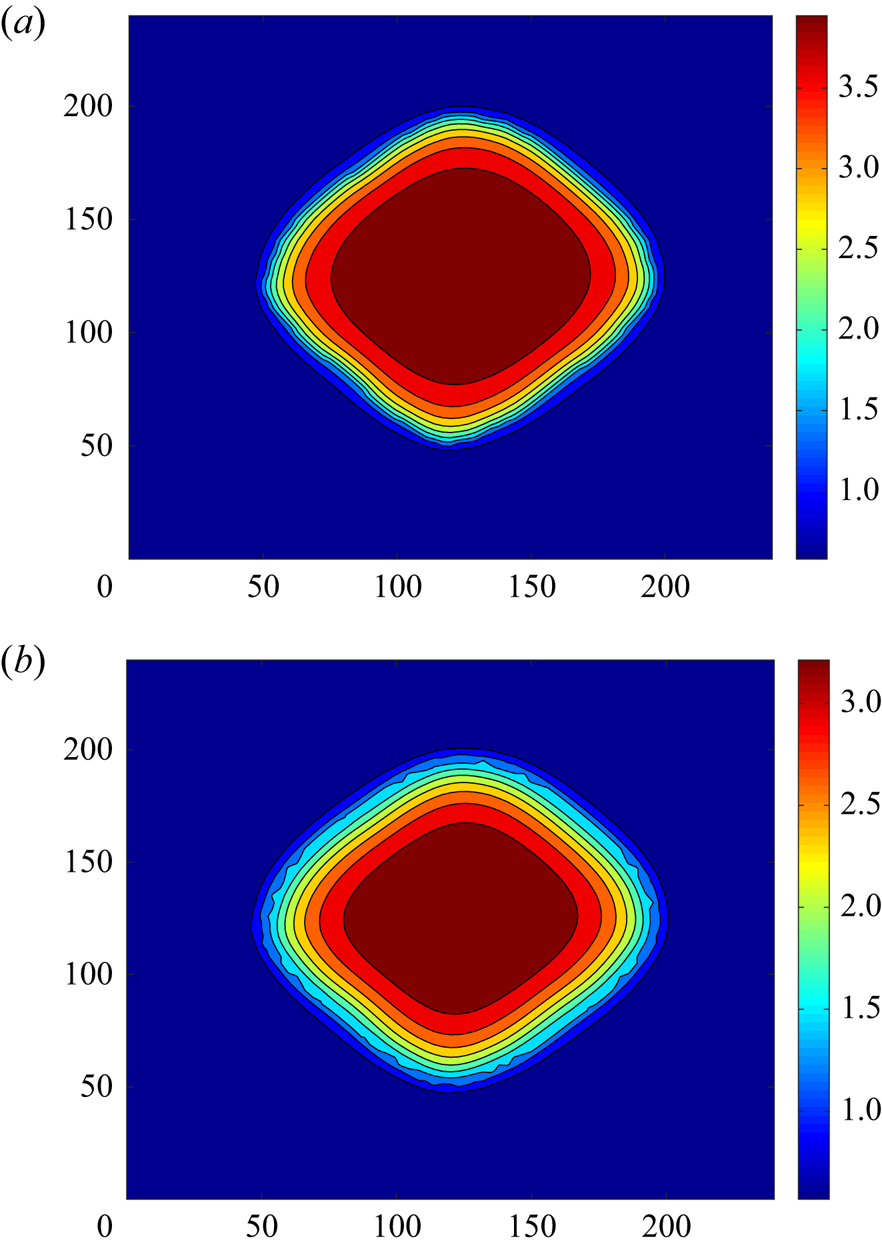
The shapes of (a) interface  $h_2(X,Y,\tau )$ and (b) interface
 $h_1(X,Y,\tau )$ for
 $\bar {M}=-4$,
 $Bo=0.05$,
 $Bi=20$,
 $A=0.75$,
 $\omega =0.00052$,
 $\tau =1\times 10^{6}$.
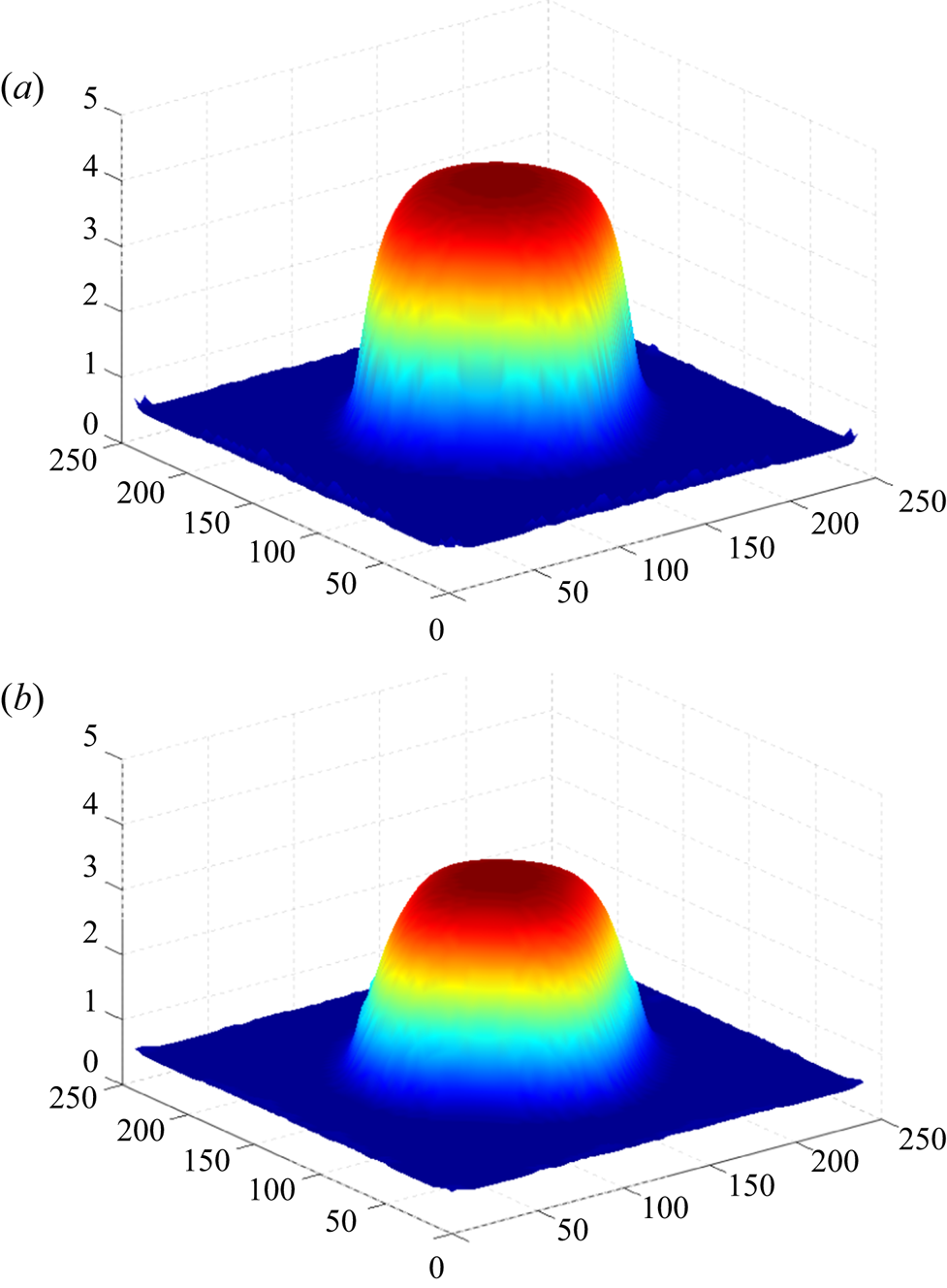
With an increase of gravity (we take  $Bo=0.2$), the amplitude of periodic oscillations essentially decreases (cf. figures 28 and 25). The shapes of interfaces
 $h_2(X,Y,\tau )$ and
 $h_1(X,Y,\tau )$ are presented in figure 29. Let us emphasize that the dependence of the liquid–gas interface height on the distance from the droplet centre becomes non-monotonic, so that this interface resembles an ‘inkpot’. The upper boundary of the droplet oscillates in the vertical direction around a nearly flat position. During part of the period, it is bent down forming an inkpot, and during another part of the period it is bent up, and thus there is no inkpot. Let us note that it is quite natural when a flat surface of the droplet with a small stationary value of
 ${\partial ^{2} h}/{\partial z^{2}}$ at the droplet's top point starts to oscillate, then during a part of the time
 ${\partial ^{2} h}/{\partial z^{2}}>0$ in the top point (and we get an inkpot) and during the rest of the time
 ${\partial ^{2} h}/{\partial z^{2}}<0$ (and there is no inkpot). Thus, the basic effect of the temporal heating modulation is a change of the droplet's shape.
The oscillations of  $h_{max,2}(\tau )$ (solid line) and
 $h_{max,1}(\tau )$ (dashed line) for
 $\bar {M}=-4$,
 $Bo=0.2$,
 $Bi=20$,
 $A=0.75$,
 $\omega =0.00052$.
The shapes of (a) interface  $h_2(X,Y,\tau )$ and (b) interface
 $h_1(X,Y,\tau )$ for
 $\bar {M}=-4$,
 $Bo=0.2$,
 $Bi=20$,
 $A=0.75$,
 $\omega =0.00052$,
 $\tau =1\times 10^{6}$.
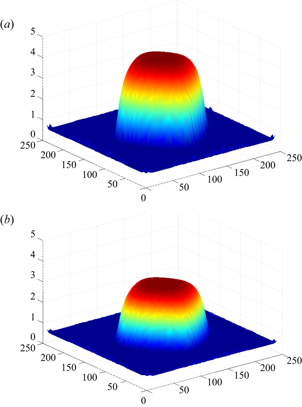
If we take the rhombic droplet shown in figures 21 and 22 as the initial condition (frequency  $\omega _{2} =4 \omega$), under the action of gravity (
 $Bo=0.05$) the amplitude of periodic oscillations decreases and the droplet is essentially flattened. A snapshot of the fields of
 $h_2(X,Y,\tau )$ and
 $h_1(X,Y,\tau )$ is shown in figure 30 and the shapes of interfaces are presented in figure 31. For sufficiently large
 $Bo$ (
 $Bo>1.2$), a ‘frozen’ steady structure develops in the system.
A snapshot of the fields of (a)  $h_2(X,Y,\tau )$ and (b)
 $h_1(X,Y,\tau )$ for
 $\bar {M}=-4$,
 $Bo=0.05$,
 $Bi=20$,
 $A=0.25$,
 $\omega =0.00104$,
 $\tau =1\times 10^{6}$.
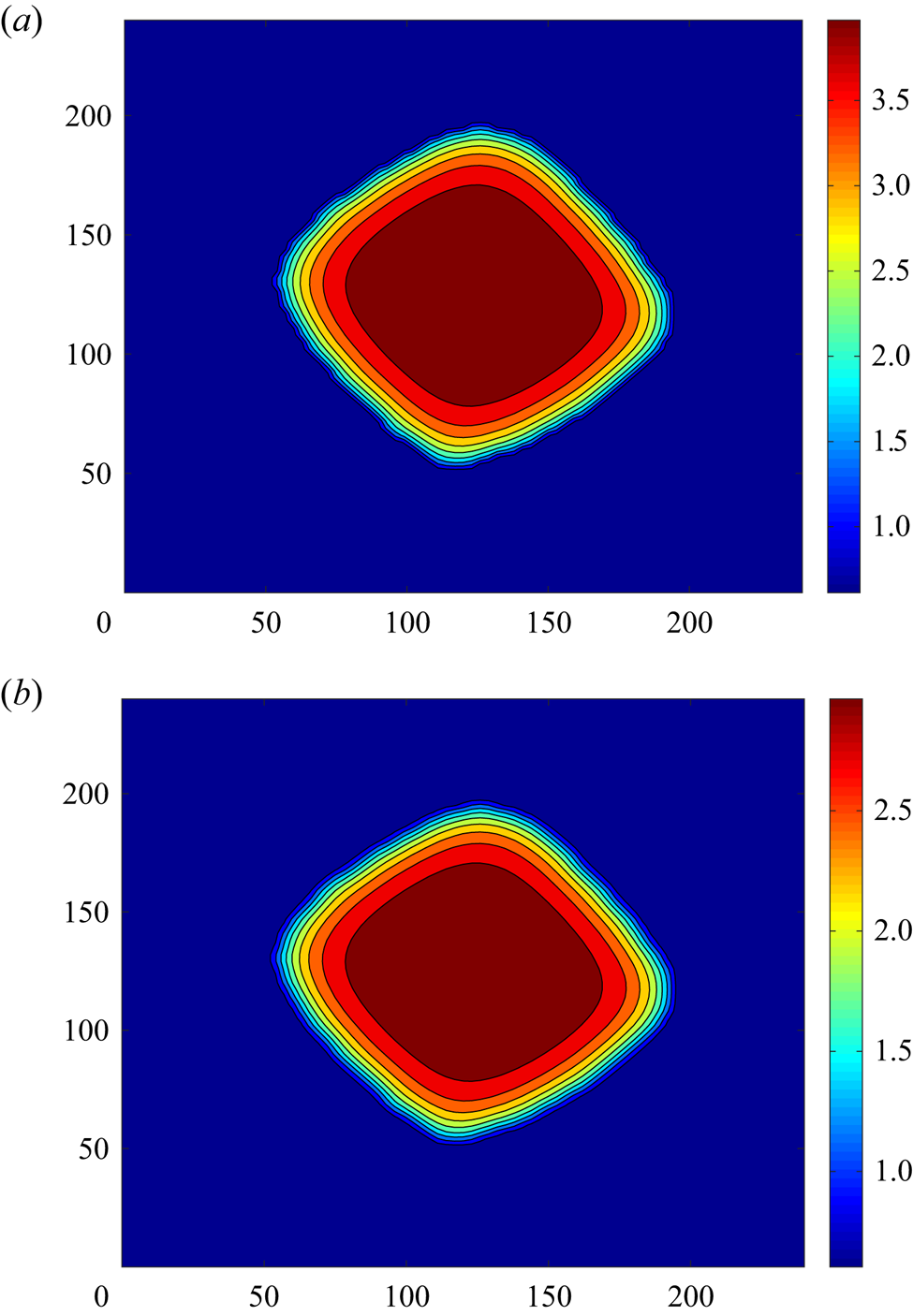
The shapes of (a) interface  $h_2(X,Y,\tau )$ and (b) interface
 $h_1(X,Y,\tau )$ for
 $\bar {M}=-4$,
 $Bo=0.05$,
 $Bi=20$,
 $A=0.25$,
 $\omega =0.00104$,
 $\tau =1\times 10^{6}$.
4. Conclusions
The influence of the temporal modulation on Marangoni instabilities of droplets on a liquid substrate has been investigated. The problem has been studied numerically in the framework of long-wave amplitude equations and precursor model. It has been shown that temporal modulation can change the droplet's shape. Specifically, rhombic droplets have been obtained. The droplet's shape influences significantly the droplet's oscillations.
The effect of gravity has been taken into account. The gravity flattens the droplet and suppresses the oscillations, ‘freezing’ the droplet's shape.
In conclusion, let us estimate the physical values of parameters needed for the observation of the phenomena described in the paper. For the values of parameters  $\eta _1=2.55\times 10^{-2}$ kg m
 $^{-1}$ s
 $^{-1}$,
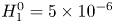 $H_1^{0}=5\times 10^{-6}$ m,
 $\sigma _1^{0}=7.6\times 10^{-3}$ N m
 $^{-1}$ and
 $L^{*}=5\times 10^{-5}$ m, applying the definition of the Marangoni number (2.3), we find that the value
 ${M=-4}$ used in our computations corresponds to a temperature difference
 $T_g-T_s=0.5$ K.
Note that time scale (3.1a,b) is equal to  $1.7\times 10^{-1}$ s. Thus, the typical dimensional frequency of droplet oscillations observed in simulations is equal to
 $1.8\times 10^{-4}$–
 $2.6\times 10^{-4}$ s
 $^{-1}$.
Funding
This research was supported by the Israel Science Foundation (grant no. 843/18).
Declaration of interests
The authors report no conflict of interest.