2.1. Flocking basics

The theoretical framework proposed by Olfati-Saber [Reference Olfati-Saber8] defines agents (real and virtual) to induce different behaviors in the control law:

• • $\alpha$ -agents are real neighbor agents that induce forces to maintain the formation.

• • $\beta$ -agents are virtual agents that enable obstacle avoidance.

• • $\gamma$ -agents are virtual agents that allow the formation navigation.

In that work, the agents are modeled by second-order particle dynamics. Each agent $i$ is ruled by a control law composed of three terms:

(1) \begin{equation} u_i=u_i^{\alpha }+u_i^{\beta }+u_i^{\gamma } \end{equation}

Each term aims to induce behaviors for the corresponding kind of agent: $u_i^{\alpha }$ is a gradient-based term to induce separation, cohesion, and alignment between $\alpha$ -agents, $u_i^{\beta }$ is a repulsion term in charge of avoiding obstacles, and $u_i^{\gamma }$ is dedicated to tracking a moving point as navigational feedback. While $\alpha$ and $\beta$ -agents are proximity agents depending on relative distances that can be represented in local reference frames, the virtual $\gamma$ -agent represents a globally defined moving rendezvous point for all the formation. The application of these navigation rules is not possible under a system with no global position reference.

2.2. Agents model

We will be considering $n$ number of homogeneous agents with second-order particle dynamics:

(2) \begin{equation} \dot {q}_i=p_i, \quad \dot {p}_i=u_i \end{equation}

where $q_i,p_i, u_i\in \mathbb{R}^m$ , are the position, velocity, and control input vectors, respectively. Each agent is defined by a unique ID and should be able to calculate its own velocity. All agents share a common global direction but not a common global positioning system; therefore, each agent uses a local reference frame oriented in a global direction.

2.3. Sensing capabilities

We assume that all agents can communicate among them through a communication network, modeled as a graph $\mathcal{G}(t)=\{\mathcal{V},\mathcal{E}(t)\}$ where $\mathcal{V}=\{1,2,\ldots ,n\}$ is the set of vertices that represent each agent and $\mathcal{E}(t)\subseteq \{(i,\,j)\mid i,\,j\in \mathcal{V},\,j\neq i\}$ is the set of edges, which represent the relations between these agents. Besides, each agent carries an omnidirectional range sensor and a compass. The agents move in an environment populated with obstacles, which will be denoted by the set $\mathcal{O}$ . The agents do not know a priori the location of the obstacles; they discover the obstacles with their sensors. The visibility capability allows the agent to visualize other agents and obstacles and calculate its relative measurements.

Each agent $i$ will generate a visibility polygon $\mathcal{P}_i$ from its position $q_i$ , and it is defined as the set of points $q$ that are visible from point $q_i$ , that is, the line segment joining $q$ and $q_i$ that has no intersection with any point of any obstacle:

(3) \begin{align} \mathcal{P}_i=\{q\in \mathbb{R}^m\mid \overrightarrow {qq}_i\cap \mathcal{O}=\emptyset \} \\[-25pt] \nonumber \end{align}

Definition 1. The perception zone of agent $i$ is denoted as $\mathcal{P}_i^{\alpha }$ , and is defined as the visibility polygon constrained by the maximum perception range,

(4) \begin{align} \mathcal{P}_i^\alpha =\{q\in \mathcal{P}_i\mid q\lt r_\alpha ^{\,max}\} \end{align}

Definition 2. Every agent $i$ can detect the other agents that lie inside the perception zone $\mathcal{P}_i$ and form the $\mathcal{N}_i$ neighborhood. This set will be called perceived neighbors,

(5) \begin{align} \mathcal{N}_i^\alpha =\{j\in \mathcal{V}\mid q_j\in \mathcal{P}_i^\alpha \} \end{align}

An agent cannot detect another agent that is blocked by an obstacle.

3.1. Agent behaviors

First, we define similar types of agents as in the flocking basics, $\alpha$ -agents, $\beta$ -agents, and $\gamma$ -agents, but with important differences with respect to existing approaches [Reference Olfati-Saber8, Reference Su, Wang and Lin17–Reference Wu, Ji, Sun, Fu and Zhao19].

3.1.1. Modeling connectivity: $\alpha$ -agents

For flocking, the agents need to form a connected graph to achieve cohesion and to build and $\alpha$ -lattice structure. Typically, existing works consider that two agents are connected if they are inside the maximum distance range $r_\alpha ^{\,max}$ . Moreover, the perception range is restricted to accomplish $\tfrac {r_\alpha ^{\,max}}{r_\alpha ^{des}}=1+\epsilon$ with $\epsilon \ll 1$ . We propose to enlarge the perception range without affecting $\alpha$ -lattice feasibility by using a Delaunay triangulation [Reference Klein23] to define the network topology. In a proximity graph, an agent’s neighborhood is defined by $\mathcal{N}_i(t)=\{j\in \,\mathcal{V}\mid r_{ij}\lt r_\alpha ^{\,max}\}$ , where $r_{ij}$ is the distance between agents $i$ and $j$ . For a large number of agents and a large perception range, the proximity graph leads to communication overload and geometric inconsistencies in forming the $\alpha$ -lattice structure. Agents that are distant and obstructed by other agents will never be able to attain the desired distance value.

A Delaunay graph $\mathcal{G}_D(t)=(\mathcal{V},\mathcal{E}_D(t))$ is a geometric structure that connects a set of points in space with nonoverlapping edges [Reference Klein23]. The basic properties that make a Delaunay graph a better choice for connectivity definition in comparison with a proximity graph are: (1) The existence of a spanning tree in the network is guaranteed. (2) There is only one Delaunay graph for a given set of points, and it can be calculated locally. (3) The empty circumcircle property, defined as any three vertices connected by edges that do not contain any other vertex inside, allows the construction of the connectivity graph. Figure 1 shows agents connected in Delaunay graphs without restrictions and with constraints imposed by obstacles and maximum distance.

Figure 1.

Agents defining Delaunay graphs. (a) Delaunay graph $\mathcal{G}_D$ without restrictions due to obstacles and maximum distance. (b) $\alpha$ -Delaunay graph built with constraints imposed by obstacles and maximum range.

3.1.2. Obstacles detection: $\beta$ -agents

The agents are not informed about the set of obstacles $\mathcal{O}$ in the environment; instead, they will identify a portion of the set when an obstacle is within their visibility range $r_\alpha ^{\,max}$ . The obstacles and agents will induce different behaviors; therefore, it becomes necessary to distinguish between obstacles and other agents within the environment.

Assumption 3. The agents are able to differentiate between obstacles and other agents.

This distinction is possible due to the information exchanged among agents through the communication network (all can communicate with each other). Each agent will explore the environment, seeking obstacles in the environment and generating a subset $\mathcal{O}_i$ based on the maximum obstacle perception range $r_\beta ^{\,max}\leq r_\alpha ^{\,max}$ . This subset may contain multiple obstacles, which are distinguishable due to distance discontinuities.

Each agent with position $q_i$ defines its own obstacles set $\mathcal{O}_i$ as follows:

(6) \begin{equation} \mathcal{O}_i=\{ q_o\in \mathcal{O} \mid \|q_i-q_o \| \lt r_\beta ^{\,max}\} \end{equation}

and can differentiate between $\kappa$ distinct obstacles $\mathcal{O}_{ik}$ , $k=\{1,\ldots ,\kappa \}$ , by detecting a distance discontinuity $\eta$ :

(7) \begin{equation} \mathcal{O}_{ik}=\{q_l \in \mathcal{O}_i|\forall q_{l}\in \mathcal{O}_{ik},\exists q_s\in \mathcal{O}_{ik}, l\neq s, \|q_l-q_s \| \leq \eta \} \end{equation}

where $q_l,q_s\in \mathcal{O}_i$ are two points from the obstacles perceived set, and obstacle point $q_l$ is considered to be part of the obstacle $\mathcal{O}_{ik}$ if there exists another point $q_s$ in that obstacle such that the distance between them is less than or equal to the distance discontinuity $\eta$ .

Each obstacle $\mathcal{O}_{ik}$ will be represented by the closest point of the obstacle to agent $i$ , and this point will form a virtual agent at the boundary of the obstacle, which will be called $\beta$ -agent. See Figure 2.

Figure 2.

Obstacles detection and definition of $\beta$ -agents.

Definition 4 ( $\beta$ -neighborhood). The set $\mathcal{N}_i^{\beta }$ of $\beta$ -agents of agent $i$ is created at the closest point between each obstacle $\mathcal{O}_k \in \mathcal{O}_i$ and agent $i$ :

(8) \begin{equation} \mathcal{N}_i^{\beta }=\{ q_o\in \mathcal{O}_{ik} \mid q_o=\text{arg}\min _{q\in \mathcal{O}_{ik}}( \| q_i-q \|) \} \end{equation}

The obstacle point $q_o$ is employed only for definition purposes; however, it is possible to directly acquire relative information about the obstacle, such as the relative distance $r_{ik}$ and angle $\theta _{ik}$ of the closest point $q_o$ . The unit vector from the agent to the closest point is given by $\hat {n}_{ik}=[\cos \theta _{ik}, \sin \theta _{ik}]^T$ . This relative information will be used by the control law for obstacle avoidance.

3.1.3. Chain-flocking: $\gamma$ -agents

In this work, due to the absence of a global positioning system, unlike existing works [Reference Olfati-Saber8, Reference Sakai, Fukushima and Matsuno18], we rely on the local perception of each agent and the information that can be exchanged within the network to define a navigation rule for every agent. We propose that agents follow each other, selecting a neighbor to track that leads them to a leader agent. This strategy is our main proposal and we call it chain-flocking.

The chain-flocking method is based on the visibility properties from the agent’s perception. Now, assume that a formation leader $\gamma _0$ has already been selected (the selection process will be described in Section 3.1.4). If all agents are connected by the $\alpha$ -Delaunay graph $\mathcal{G}_{\alpha D}$ , which posses the visibility constrains of Def. 1 (see Figure 3a), then each agent $i\in \mathcal{V}$ can find a graph path within $\mathcal{G}_{\alpha D}$ that is free of obstacles connecting with the leader $\gamma _0$ . This is illustrated in Figure 3b, where it is visible that each connected agent can keep on track of the leader by tracking its own neighbor. Consequently, if the leader is informed about a path that is free of obstacles, then each follower agent is able to navigate the same path as the leader by indirectly tracking it through a neighbor that connects with it. This neighbor will be called $\gamma$ -agent, and each agent $i$ identifies its own $\gamma _i$ -agent to follow. To do so, two criteria must be considered: (1) avoid risk of collision with any other agents during the tracking, and 2) select the nearest neighbor to the leader within the formation graph.

Figure 3.

Visibility and chain path for navigation of the MAS. (a) Perception zone. (b) Chain path toward the leader.

To address the first criteria, the Gabriel graph proximity notion is introduced. Risk of collision is avoided by introducing a constraint in the agents’ connectivity to form a new graph called the Gabriel graph, formed theoretically as the intersection of the edges of the Delaunay graph and the Voronoi diagram. In practice, the condition for connecting two agents in the Gabriel graph is to establish a region of influence where no other agent should reside, as illustrated in Figure 4. This region is defined by a circle with center at the midpoint of the two agents and circumscribed by them. The neighbors that fulfill the Gabriel condition will be called Gabriel neighbors $\mathcal{N}_i^{\alpha G}$ .

Figure 4.

Gabriel condition of Def. 5. (a) Condition not fulfilled: agent $\gamma _0\notin \mathcal{N}_i^{\alpha G}$ , as the region of influence between $\gamma _0$ and $\alpha _i$ is occupied by $\alpha _j$ . (b) Condition fulfilled: agent $\alpha _j\in \mathcal{N}_i^{\alpha G}$ , as the region of influence between $\alpha _i$ and $\alpha _j$ is free.

Definition 5 (Gabriel neighborhood [Reference Mesbahi and Egerstedt24]). Given a neighbor $j \in \mathcal{N}_i^{\alpha D}$ of agent $i$ , $j$ will be part of the Gabriel neighborhood $\mathcal{N}_i^{\alpha G}$ if there exists a circle $c$ with center at the midpoint $h = \tfrac {q_i-q_j}{2}$ and circumscribed by agents $i$ and $j$ , such that there is no other agent $l \in \mathcal{N}_i^{\alpha D}$ positioned inside the circle $c$ , that is:

(9) \begin{equation} \mathcal{N}_i^{\alpha G}= \{ j \in \mathcal{N}_i^{\alpha D} | \,\forall l \neq j \in \mathcal{N}_i^{\alpha D}, \|h-q_j\| \leq \|h-q_l\| \} \end{equation}

This set will be used by each agent $i$ to find its $\gamma$ -agent to follow. Once the collision avoidance criterion has been established, the agent to follow $\gamma _i$ must comply with the nearest neighbor criterion. The nearest neighbor is defined as the neighbor with the minimum distance toward the leader agent $\gamma _0$ within the formation graph $\mathcal{N}_i^{\alpha G}$ . This criterion is evaluated by using the distances between agents as the weights of the graph edges to allow the search for the shortest path in distance inside the graph. As every agent knows only local information about their neighbors, the shortest path length is computed in a distributed manner using distances shared through the communication network.

The shortest path length $r_{i \gamma _0}^*$ of agent $i$ is calculated by expanding the shortest path length $r_{j \gamma _0}^*$ of a neighbor $j$ by adding the sensing distance to the neighbor $r_{ij}$ , and finding the minimum among all expanded paths through the graph. See example in Figure 5a.

Figure 5.

Shortest path length. (a) Example of computation. (b) $\gamma _i=\gamma _0$ , as there are no obstacles. (c) $\gamma _i=\alpha _j$ , as there is one obstacle.

By using the shortest path length over the Gabriel Graph neighbors $j\in \mathcal{N}_i^{\alpha G}$ , we address both restrictions for the selection of the $\gamma _i$ -agent: avoiding collisions with neighbors and ensuring proximity to the leader. However, the collision avoidance restrictions are relaxed when there are no obstacles sensed by the agent $\mathcal{N}_i^{\beta }\neq \emptyset$ , as even if the agent passes near another agent, it has free space to avoid collision, which is not the case when there are obstacles near the agent. This difference is illustrated in Figure 5b, c. Then, each agent can obtain its $\alpha$ -agent by applying the following definition:

Definition 6 ( $\gamma$ -agent). The $\gamma$ -agent of agent $i$ is its neighbor $j$ that belongs to Gabriel neighborhood $j \in \mathcal{N}_i^{\alpha G}$ when there are sensed obstacles $\mathcal{N}_i^{\beta }\neq \emptyset$ , or to the $\alpha$ -Delaunay neighborhood $j \in \mathcal{N}_i^{\alpha D}$ otherwise, and that has the shortest path length to the leader agent $\gamma _0$ . This is described as:

(10) \begin{align} \gamma _i= \begin{cases} \text{arg}\min _{j \in \mathcal{N}_i^{\alpha G}}\big(r_{j\gamma _0}^*+r_{ij}\big), \\[4pt] \text{arg}\min _{j \in \mathcal{N}_i^{\alpha D}}\big(r_{j\gamma _0}^*+r_{ij}\big), \end{cases} \end{align}

where $r_{j\gamma _0}^*$ is the shortest path length of neighbor $j$ to the leader $\gamma _0$ , which is received through communication, and $r_{ij}$ is the distance to the neighbor $j$ sensed by the agent $i$ .

Now, we can define the formation graph given by the $\gamma$ -agents by considering all the relations between each agent and its $\gamma _i$ -agent.

Definition 7 (Chain graph). The chain graph $\mathcal{G}_C(\mathcal{V},\mathcal{E}_C)$ is a directed spanning tree with root node at the leader agent $\gamma _0$ , which allows the distribution of the information from the leader to every agent $i\in \mathcal{V}$ . The edges of this graph are defined as $\mathcal{E}_C=\{(i,\gamma _i), \forall i\in \mathcal{V}\}$ , that is, the edges that connect every agent $i$ with its corresponding $\gamma$ -agent. For instance, see the yellow edges in Figure 5b , c .

3.1.4. Navigation $\gamma _0$ -agent (leader)

To avoid the dependence of a predefined leader–follower formation, we propose to select as leader the best-suited agent toward the goal. This can be achieved assuming that all agents must be informed about the desired goal. Besides, the agents must be capable of sharing their information among their neighbors, so they can compare with each other and determine the best-positioned agent relative to the goal.

We propose a method for selecting a formation leader in a distributed manner. A cost function $J^g$ is used to identify the agent with the minimum cost toward the goal. The selected leader will have a motion planning strategy to navigate toward the goal. The definition of the cost to goal criteria $J^g$ will depend on information data from the environment, such as estimated path error to goal, passage sizes, obstacle sizes, etc. The cost function $J^g$ and the motion planning strategy will be described later in Section 3.3.

Definition 8 (Leader $\gamma _0$ ). The formation leader is the agent $i \in \mathcal{V}$ whose cost function $J_i^g$ is the minimum of all agents, that is:

(11) \begin{equation} \gamma _0=i=\text{arg}\min _{i\in \mathcal{V}}(J_i^g) \end{equation}

The agents cannot evaluate the cost function directly, as they only communicate with their neighbors. To select the leader, each agent $i$ compares the cost shared by their neighbors $J_i^g$ to find the agent with the minimum cost $J_i^{g*}$ among them all, including itself. 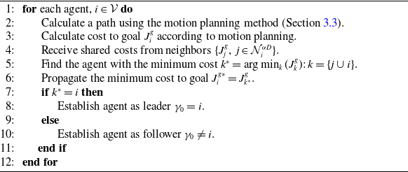If the agent $i$ founds itself as the minimum cost agent, then it becomes the formation leader and the propagated cost will be equal to its own cost $J_i^{g*}=J_i^g$ ; otherwise, the agent will propagate to its neighbors $j$ the cost of a neighbor, or even the cost of an agent that is not within the perception range of agent $i$ , whose cost is the minimum. This enables the agents to propagate the cost of the best-suited neighbor throughout the entire formation. This formulation is detailed in Alg. 1.

Algorithm 1.

Leader selection

Algorithm 1 Long description

An algorithm for leader selection among agents based on cost comparison. The algorithm involves several steps for each agent. First, a path is calculated using a motion planning method. Next, the cost to the goal is calculated according to the motion planning. The agent then receives shared costs from its neighbors. The agent identifies the neighbor with the minimum cost and propagates this minimum cost to the goal. If the agent itself has the minimum cost, it establishes itself as the leader. Otherwise, it establishes itself as a follower. This process is repeated for each agent.

3.2. Control algorithm

Every agent $i\in \mathcal{V}$ applies a control input with the three components of Eq. 1, where each term determines the particular behavior induced by each agent type: $\alpha$ -control for formation, $\beta$ -control for obstacle avoidance, and $\gamma$ -control for navigation. These control laws are inspired by the work in ref. [Reference Olfati-Saber8], but an important difference is that each control term uses local measurements obtained from onboard distance sensors. Moreover, the behavior of the flocking navigation is really different from the one in ref. [Reference Olfati-Saber8], as was described in Section 3.1.3.

3.2.1. $\alpha$ -control (formation)

The purpose of the control term $u_i^{\alpha }$ is to drive the agents to form an $\alpha$ -lattice structure. The $\alpha$ -control is composed of two terms; the first one is a gradient-based term, and the second one is a consensus-based term:

(12) \begin{align} u_i^\alpha = \frac {1}{|\mathcal{N}_i^{\alpha D}|} \left \{ \kappa _g^\alpha \sum _{j\in \mathcal{N}_i^{\alpha D}}\phi _\alpha (d_{ij})\hat {n}_{ij} + \kappa _p^\alpha \sum _{j\in \mathcal{N}_i^{\alpha D}} a(d_{ij})(p_j-p_i) \right \} \end{align}

where $\kappa _g^\alpha , \kappa _p^\alpha \gt 0$ are control gains, gradient and proportional, respectively, $d_{ij}=\| r_{ij} \|_\sigma$ is the distance between agents $\alpha _i$ and $\alpha _j$ under a $\sigma$ -norm (see [Reference Olfati-Saber8]), and $\hat {n}_{ij}$ is the unit vector connecting those agents. $\phi _\alpha (z)$ and $a(z)$ are adequate functions to define the potentials as in ref. [Reference Olfati-Saber8]. The action function $\phi _\alpha (z)$ will drive the agents to a desired inter-distance $r_\alpha ^{des}$ . To avoid inter-agent collision for agents with a body, the body size radius $r_\alpha ^{size}$ needs to be considered in the selection of the desired distance between agents such that $r_\alpha ^{size}\lt r_\alpha ^{des}\lt r_\alpha ^{\,max}$ .

3.2.2. $\beta$ -control (obstacle avoidance)

The control term $u_i^\beta$ allows the agents to avoid the obstacles in the environment. It creates a repulsive artificial potential field at the closest point of each perceived obstacle. The $\beta$ -control is only composed of a gradient-based term:

(13) \begin{equation} u_i^\beta =\kappa _g^\beta \frac {1}{|\mathcal{N}_i^{\beta }|} \sum _{k\in \mathcal{N}_i^{\beta }} \phi _\beta (d_{ik}) \hat {n}_{ik} \end{equation}

where $\kappa _g^\beta \gt 0$ is a control gain for the gradient, $d_{ik}=\| r_{ik} \|_\sigma$ is the distance between agents $\alpha _i$ and $\beta _{ik}$ under a $\sigma$ -norm, and $\hat {n}_{ik}$ is the unit vector connecting those agents. $\phi _\beta (z)$ is an adequate function to define the potentials as in ref. [Reference Olfati-Saber8]. The action function $\phi _\beta (z)$ will drive the agents to a desired distance from obstacles $r_\beta ^{des}$ , generating a repulsive force when the distance falls below the designated threshold. To avoid collision with obstacles for agents with a body, the body size radius $r_\alpha ^{size}$ needs to be considered in the selection of the security distance between agents and obstacles such that $r_\alpha ^{size}\lt r_\beta ^{des}\lt r_\beta ^{\,max}$ .

3.2.3. $\gamma$ -control (navigation)

The control term $u_i^\gamma$ is different for the leader agent $i=\gamma _0$ and followers $i\neq \gamma _0$ , each case is defined next.

–Followers control: The purpose of the control term $u_i^\gamma$ is to follow the $\gamma$ -agent selected by the method of Section 3.1.3. This term will lead indirectly the agent $i$ toward the leader $\gamma _0$ . The control law will maintain the neighbor agent $i$ at a desired distance $r_\gamma ^{des}=r_\alpha ^{des}$ while tracking its velocity $p_{i\gamma }$ . This control law drives the agents to form the chain-flocking structure. The $\gamma$ -control is composed of two terms, a gradient-based term and a velocity consensus term:

(14) \begin{equation} u_i^\gamma =\kappa _g^\gamma \,\phi _\gamma (d_{i\gamma }) \hat {n}_{i\gamma } + \kappa _p^\gamma \,c(d_{i\gamma }) \big(p'_{i\gamma }-p_i\big) , \quad i\neq \gamma _0 \end{equation}

where $\kappa _g^\gamma , \kappa _p^\gamma \gt 0$ are control gains, gradient and proportional, respectively, $d_{i\gamma }=\| r_{i\gamma } \|_\sigma$ is the distance between agents $\alpha _i$ and $\gamma _i$ under a $\sigma$ -norm, $\hat {n}_{i\gamma }$ is the unit vector connecting those agents and $p'_{i\gamma }$ is a target velocity vector that will be defined later. $\phi _\gamma (z)$ and $c(z)$ are adequate functions to define the potentials as in ref. [Reference Olfati-Saber8].

The main goal of the control $u_i^\gamma$ is to drive each follower toward its corresponding $\gamma _i$ -agent with velocity vector $p_{i\gamma }$ to achieve the chain-flocking behavior. However, to deal also with obstacles, the velocity $p_{i\gamma }$ must be deviated by the obstacles perceived $\mathcal{N}_i^{\beta }$ , resulting in the following target velocity:

(15) \begin{align} p'_{i\gamma }= \begin{cases} \tfrac {1}{|\mathcal{N}_i^{\beta }|}\sum _{k\in \mathcal{N}_i^{\beta }}\left \{ b(\bar {\theta }_{ik},d_{ik})p_{ik} +(1-b(\bar {\theta }_{ik},d_{ik}))p_{i\gamma } \right \},\,\mathcal{N}_i^{\beta } \neq \emptyset \\[3pt] p_{i\gamma }, \quad \hspace {6.3cm} \mathcal{N}_i^{\beta }=\emptyset \end{cases} \end{align}

where $b(\bar {\theta }_{ik},d_{ik})\in [0,1]$ is a function that allows the smooth transition between the $\gamma _i$ agent’s velocity $p_{i\gamma }$ and the virtual obstacle velocity $p_{ik}$ and is defined as $b(\bar {\theta }_{ik},d_{ik})=\rho _{h_\theta }\left (\tfrac {\bar {\theta }_{ik}}{(2/3)\pi }\right )\rho _{h_\beta }\Bigl (\tfrac {d_{ik}}{d_\beta ^{\,max}}\Bigr )$ , where $\rho _{h}$ are bump functions as in ref. [Reference Olfati-Saber8], with $d_{ik}=\|d_{ik}\|_{\sigma }$ the distance between agent $i$ and its $\beta$ -agent $\beta _{ik}$ , $d_\beta ^{\,max}=\|r_\beta ^{\,max}\|_\sigma$ the maximum obstacle detection range, both under the $\sigma$ -norm. The parameter $\bar {\theta }_{ik}$ is the angle between the agent’s direction $\hat {n}_i$ and the obstacle’s direction $\hat {n}_{ik}$ , which is given by $\bar {\theta }_{ik}=\cos ^{-1}(\hat {n}_i \cdot \hat {n}_{ik})$ . The function $b(\bar {\theta }_{ik},d_{ik})$ allows an agent to overlook an obstacle when it is too far or when the agent is not navigating toward it.

In addition, each agent $\beta _{ik}$ will create a virtual velocity $p_{ik}$ to deviate the velocity $p_{i_\gamma}$ with the same magnitude, but perpendicular to the obstacle agent’s direction $\hat {n}_{ik}$ , that is:

(16) \begin{equation} p_{ik}=s_{ik} \hat {n}_{ik}^\perp \|p_{i_\gamma }\| \end{equation}

where $s_{ik}$ allows the correct selection of the direction of the target velocity; $s_{ik}=1$ if $\cos ^{-1}\big(\hat {n}_{ik}^\perp \cdot \hat {n}_{i_\gamma }\big)\leq \tfrac {\pi }{2}$ , and $s_{ik}=-1$ otherwise, with $\hat {n}_{ik}^\perp$ the vector perpendicular to the obstacle and $\hat {n}_{i_\gamma }$ the vector pointing to the $\gamma _i$ agent.

–Leader control: We define a control law that requires only a velocity vector to guide the leader agent through the environment, not depending on a global positioning system. The $\gamma$ -control of the leader is composed of one term that is a velocity tracking function defined as:

(17) \begin{equation} u_i^{\gamma }=\kappa _p^{\gamma _0} (p_{i}^g-p_i), \quad i=\gamma _0 \end{equation}

where $\kappa _p^{\gamma _0}\gt 0$ is a control gains. The velocity target $p_{i}^g$ is calculated by the motion planning scheme, which is described in the following section.

Notice that an important difference between Olfati-Saber’s method [Reference Olfati-Saber8] and the proposed method is that $u_i^\gamma$ are defined differently. In our method, the leader’s motions deform the lattice, since each agent has a local leader, who is following, defined by a planning method. When the global leader reaches the goal, it is motionless, and eventually, each local leader will be motionless. At that time, the approach becomes exactly the same as the Olfati-Saber’s one. Hence, the convergence of the formation is guaranteed when the goal is reached, similarly to the Olfati-Saber’s method.

3.3. Motion planning

To allow the navigation of the agents without a global positioning system, we proposed the use of a reactive navigation method, the so-called ND [Reference Minguez and Montano9]. We underline that it is possible to change only the motion planning method, adapted to our multi-agent scenario, while keeping the same control scheme. The main goal of the motion planning method is to obtain the target velocity vector for the leader and the metrics to select the leader using Alg. 1. The ND is a reactive obstacle avoidance method for 2D space, proposed in ref. [Reference Minguez and Montano9].

In this work, we have extended the ND method to multiple agents. We use the so-called $\alpha$ -shape structure [Reference Edelsbrunner, Kirkpatrick and Seidel25] to find the frontier of the formation under range constraints ( $\alpha =r_\alpha ^{\,max}/2$ ) since agents in the frontier have clear visibility of the environment. The $\alpha$ -shape is a generalization of the convex hull, described as the smallest geometric structure that encloses a set of points in space, given a maximum distance between agents.

Using the $\alpha$ -shape, formation regions are calculated. A formation region is composed of intervals of angles indicating the inside of the formation, which are clearly not traversable sectors. An example of a formation region is illustrated in Figure 6a. For agents with a body, it is necessary to define neighbor regions that consider the agents’ size. An example of a neighbor region is shown in Figure 6b where it is visible that the region is expanded as the agent’s size increases.

Figure 6.

Formation and neighbor’s regions. (a) Formation region $\Theta _i^F$ of agent $i$ . (b) Neighbor’s regions $\Theta _i^N$ of agent $i$ .

To avoid collision with moving agents and using the formation and neighbor regions, we propose the Formation Nearness Diagram (FND) from the central point, which is an extension of the PND,Footnote ¹ as defined in ref. [Reference Minguez and Montano9]. To detect obstacles in the FND, depth discontinuities (called gaps) are found. In the FND, when moving agents are close, blocking a path, they are merged together, creating a virtual obstacle. See Gap F in Figure 7. As in the original ND, valleys are formed by two discontinuities or gaps created by the obstacles in the environment. But in this work, to deal with moving agents that can block a path, a valley is not traversable if a circle formed between the agent and an obstacle’s gap is not empty. See Figure 7. By applying the criteria on traversability defined in ref. [Reference Minguez and Montano9] to our FND, the result is a navigation sector $s_{\theta }$ with direction angle $\varphi _{\theta }$ . This sector is collision-free and is related to the traversable valley that is closest to the goal direction.

The ability to change leaders ensures that at least one robot will always find a collision-free path to the goal if the path exists; then, as the robots move following the leader, they find a traversable valley.

We left for future work to extend the planner to the 3D case. However, an advantage of our method is that other planners capable of handling 3D obstacles can be used, as we will show in the implementation results. In other words, the proposed method is not limited to a particular planner.

Figure 7.

Formation Nearness Diagram (FND), traversable and no-traversable valleys. Valleys in red are not traversable.

3.3.1. Cost function for leader selection

As described in Section 3.1.4 and in Alg. 1, now we can define a cost function considering the features of the proposed planning method. Eq. 18 establishes the proposed cost function.

(18) \begin{eqnarray} J_i^g(\theta _i^g,r_i^g,ID_i)=w_{\theta }|\varphi _{\theta }-\theta _i| +w_{\theta _g}|\varphi _{\theta }-\theta _i^g|+w_r\Big(r_i^g-\min _{i \in V} r_i^g\Big)+P + w_{ID}ID_i \end{eqnarray}

where $w_{\theta },w_{\theta _g},w_r, w_{ID} \in \mathbb{R}$ are positive constants that define the weight for each term. The selection of the weights affects the following priorities:

1. 1. $w_{\theta }$ minimizes path error to the current direction $|\varphi _i-\theta _i|$ ; preferring agents that calculate a navigation path that does not deviate the agent from its current direction. $\varphi _{\theta }$ is the navigation direction given by the motion planner, and $\theta _i$ is the $i$ -th agent’s heading in the global frame given by the onboard compass.

2. 2. $w_{\theta _g}$ minimizes path error to the goal $|\varphi _{\theta }-\theta _i^g|$ ; preferring agents that calculate a navigation direction with less error angle toward the goal. $\theta _i^g$ is the heading of agent $i$ with respect to the goal.

3. 3. $w_r$ minimizes the distance to goal $r_i^g$ ; preferring agents closer to the goal. A normalization to this term is applied with the minimum formation distance $\min _{i \in V} r_i^g$ .

4. 4. $P$ is a real number which is determined experimentally to keep consistency – when a new agent is better positioned toward the goal, it should outperform the previous agent to change the leader. A penalty cost $P$ is added when the $ID_i$ at time $t$ differs from the past selection at time $t-1$ .

5. 5. $w_{ID}ID_i$ is a term used as a way to select a single agent when there is a tie among more than one agent. $ID_i$ is an integer number indicating the robot identity label.

Regarding the first two terms of $J_i^g$ involving differences of angles, we calculate the minimum angle that a robot needs to rotate to aim the desired orientation.

3.3.2. Goal velocity vector

Once a leader agent is selected, the goal velocity vector $p_i^g$ required in Eq. 17 is determined from the result of the FND. The goal velocity vector is defined as:

(19) \begin{equation} p_i^g=v_{des}\,\hat {n}_i^g \end{equation}

where $v_{des}\in \mathbb{R}$ is a desired velocity magnitude and $\hat {n}_i^g$ is a unit vector with the direction to goal derived from the solution sector with direction $\varphi _{\theta }$ given by $\hat {n}_i^g=[\cos \varphi _{\theta }, \sin \varphi _{\theta }]^T$ .

4.1. Model of agents

We consider differential-drive robots that are modeled by the unicycle kinematics:

(20) \begin{align} \begin{bmatrix} \dot {x}_i \\[2pt] \dot {y}_i \\[2pt] \dot {\theta }_i \end{bmatrix} = \begin{bmatrix} \cos \theta _i & 0 \\[2pt] \sin \theta _i & 0 \\[2pt] 0 & 1 \end{bmatrix} \begin{bmatrix} v_i \\[2pt] \omega _i \end{bmatrix} \end{align}

where $x_i,y_i$ are the position coordinates of the robot’s center and $\theta _i$ its heading in a global reference frame, $v_i$ and $\omega _i$ are its linear and angular velocities, respectively. To have a model as in Eq. 2, we use a displaced control point described as:

(21) \begin{align} \begin{bmatrix} x_i^c \\[2pt] y_i^c \end{bmatrix} = \begin{bmatrix} x_i+l \cos \theta _i \\[2pt] y_i+l \sin \theta _i \end{bmatrix} \end{align}

with $l\neq 0$ a distance along the longitudinal axis of the robot.

The kinematics of the displaced control point are given by:

(22) \begin{align} \dot {q}_i = M_i \begin{bmatrix} v_i \\[2pt] \omega _i \end{bmatrix} = p_i \end{align}

where $M_i=\begin{bmatrix} \cos \theta _i & -l\sin \theta _i \\ \sin \theta _i & l\cos \theta _i \end{bmatrix}$ . Then, the vector of velocity inputs $w_i=[v_i,\omega _i]^T$ are obtained as:

(23) \begin{equation} w_i=M_i^{-1}p_i. \end{equation}

Since our flocking control scheme provides the acceleration $u_i$ , according to Eq. 2, $p_i$ can be computed by numerical integration of $\dot {p}_i=u_i$ in order to get the robot’s velocity inputs.

For simulation purposes, we use as agents the robots TurtleBot3, equipped with a 360-degree LiDAR (range of 5 m and resolution of 0.5 deg) and an Inertial Measurement Unit (IMU) to provide velocity and orientation estimation. These robots are small size, diameter $r_{\alpha }^{size}=0.13$ m, and we consider maximum linear velocity $v_{max}=0.22$ m/s and maximum angular velocity $\omega _{max}=0.8$ rad/s. To define the displaced control point, we set $l=0.05$ m, and the velocity inputs are computed every $\Delta t=0.05$ s.

4.2. Parameters of the flocking algorithm

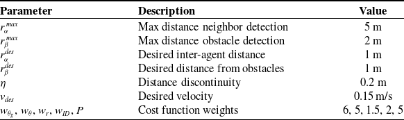
The proposed approach uses some parameters, which are listed in Table I.

Table I.

Parameters used in the simulation results.

Table I Long description

The table presents parameters used in simulation results, organized into three columns: Parameter, Description, and Value. The table has 8 rows and 3 columns. Row 1: Parameter, Description, Value. Row 2: r_alpha_max, Max distance neighbor detection, 5 m. Row 3: r_beta_max, Max distance obstacle detection, 2 m. Row 4: r_alpha_des, Desired inter-agent distance, 1 m. Row 5: r_beta_des, Desired distance from obstacles, 1 m. Row 6: eta, Distance discontinuity, 0.2 m. Row 7: v_des, Desired velocity, 0.15 m/s. Row 8: w_theta_g, w_theta, w_r, w_ID, P, Cost function weights, 6, 5, 1.5, 2, 5.

4.3. Performance metrics and $\alpha$ -flocking

The performance metrics used to evaluate the approach and to compare it with other related works are four:

1. 1. Algebraic connectivity $\lambda _2(t)$ : It is the second-smallest eigenvalue of the Laplacian matrix $L$ obtained from the interaction matrix [Reference Olfati-Saber and Murray27].

2. 2. Deviation energy $E(t)$ : It is a measure of the deviation of the formation from the $\alpha$ -lattice, determined by the following equation:

   (24) \begin{equation} E(t)=\frac {1}{(|\epsilon _{\alpha D}(t)|+1)}\sum _{i=1}^{n}\sum _{N_i^{\alpha D}} \kappa _{g}^{\alpha }\psi _{\alpha }(d_{ij}) \end{equation}
   where $\psi _{\alpha }(d_{ij})$ is the integral of the action function $\phi _\alpha (d_{ij})$ in Eq. 12, $|\epsilon _{\alpha D}(t)|$ is the size of the $\alpha$ -Delaunay graph. The gain $\kappa _{g}^{\alpha }$ used in Eq. 12 is added here to consider the real potential energy applied to the control law.

3. 3. Cohesion radius $R(t)$ : It is defined by the following expression: $\max _{i \in \mathcal{V}}||q_i(t)-q_c(t)||$ , where $q_c(t)=\frac {1}{n}\sum _{i=1}^n q_i$ .

4. 4. Velocity mismatch $K(t)$ : It is defined by the following equation:

   (25) \begin{equation} K(t)=\frac {1}{n}\sum _{i=1}^n ||p_i-p_c||^2 \end{equation}
   where $p_c(t)=\frac {1}{n}\sum _{i=1}^n p_i$ .

To verify that our algorithm generates a flocking formation, we will use the definition of an $\alpha$ -flocking presented in the Olfati-Saber’s approach [Reference Olfati-Saber8], which is based on the performance metrics presented above, it states: A group of $n$ agents perform $\alpha$ -Flocking over the time interval $[t_0,t_f]$ , if there exist relatively small numbers $\epsilon _0,\epsilon _1,\epsilon _2\gt 0$ and distance $d\gt 0$ such that the trajectory satisfies all the following conditions for all $t \in [t_0,t_f]$ , with an interaction range $r=(1+\epsilon _0)d$ : (1) The group remains a quasi-flock. (2) The group remains cohesive. (3) The deviation energy remains small $E(t) \leq \epsilon _1d^2$ . (4) The velocity mismatch remains small $K(t) \leq \epsilon _1 n$ . In this work, the variables $r$ and $d$ are referenced as $r=r_{\alpha }^{\max }$ and $d=r_{\alpha }^{des}$ , which are the interaction range and desired inter-agents’ distance, respectively.

There are two main differences of our method compared with Olfati-Saber’s approach: (1) the proposed method includes a motion planner to establish a goal for the global leader, and (2) it uses local leaders that move the agents toward them. Those innovations are the main contributions of our work. Furthermore, the proposed approach offers improvements compared with Olfati-Saber’s model. The proposed approach is able to deal with non-convex obstacles, and it is able to deform the formation to pass through narrow passages. These capabilities are clearly shown in the simulation results presented in the next sections.

4.4. Free space

The algorithm implementation is first tested in free space with $n=20$ agents, with random initial positions and headings for each agent. The agent’s velocity at start time is zero. The goal position provided to the agents is the position $q_g=(0,15)$ meters.

The evolution of the formation is shown in Figure 8 through snapshots at different simulation times. The leader agent is highlighted in yellow. The edges of the $\alpha$ -Delaunay graph are depicted with black lines connecting neighboring agents. The $\gamma _i$ agent relationship is indicated with a yellow line. The leader agent is chosen using Alg. 1, applying the cost function specified in Eq. 18.

Figure 8.

Simulation snapshots for 20 agents in free space.

The control inputs provided to each agent can be visualized in Figure 9. In that figure, it is shown that the leader agent converges to the desired velocity $v_{des}$ ; however, the leader is collaborative and adapts its velocity due to the lattice control $u_i^{\alpha }$ term.

Figure 9.

Velocity inputs for the agents in simulation in Figure 8.

Figure 9 Long description

The image contains two line graphs depicting the velocity inputs for agents in a simulation. Panel A: The top line graph shows the linear velocity over time. The x-axis represents time in seconds, ranging from 0 to 200 seconds. The y-axis represents linear velocity in meters per second, ranging from -0.1 to 0.2 meters per second. The graph includes two data series: one for the leader (in blue) and one for the followers (in gray). The linear velocity of the leader and followers increases rapidly at the beginning, stabilizes around 0.1 meters per second, and then drops sharply around the 120-second mark, after which it fluctuates near zero. Panel B: The bottom line graph shows the angular velocity over time. The x-axis represents time in seconds, ranging from 0 to 200 seconds. The y-axis represents angular velocity in radians per second, ranging from -1 to 1 radians per second. Similar to the linear velocity graph, this graph includes two data series: one for the leader (in blue) and one for the followers (in gray). The angular velocity of the leader and followers shows initial fluctuations, stabilizes around zero, and then exhibits minor fluctuations after the 120-second mark.

Figure 10.

Performance metrics for the simulation of 20 agents in free space.

The follower agents increase their velocity until they reach the desired inter-agent’s distance with their $\alpha$ -neighbors and $\gamma$ -agent. Then, they decrease their velocity to match their $\gamma$ -agent’s velocity, which is the chain formation consensus velocity $v_{des}$ . As can be seen in Figure 9, the leader reaches the goal around $112s$ , it stops, and the velocity of the followers converges around zero.

Figure 10 shows graphics of the performance metrics described in Section 4.3. The first clear difference from the Olfati-Saber’s framework [Reference Olfati-Saber8] is that our interaction range is not bounded by the restriction $r=(1+\epsilon _0)d$ . Our formation fulfills the $\alpha$ -flocking for any values of $\epsilon _0$ , as long as condition $r_{\alpha }^{des}\lt r_{\alpha }^{\max }$ is fulfilled. In our simulation configuration, the interaction range ratio is $\epsilon _0=4$ , while in Olfati-Saber’s work, a low ratio of $\epsilon _0=0.2$ is necessary to fulfill these conditions.

The accomplishment of $\alpha$ -flocking condition 1), referring to the quasi-flock formation, is shown in Figure 10. The connectivity graph $\lambda _2(t)$ increases as the simulation time progresses, and therefore, the graph remains connected for all $t \in [t_0,t_f]$ .

The condition 2), which refers to the formation cohesion, is shown to be fulfilled in the plot of the Cohesion radius $R(t)$ , where the formation radius decreases to a low value.

For the last two conditions for $\alpha$ -flocking, it is necessary to define a value for $\epsilon _1$ and $\epsilon _2$ constants. These constants are not bounded to any specific value; they are only required to be relatively small numbers. Figure 10 shows the evolution of energy deviation $E(t)$ and velocity mismatch $K(t)$ .

The energy deviation values at start and end time are $E(t_0)\approx 7.375$ and $E(t_f) \approx 0.176$ , respectively. These values give the constant $\epsilon _1$ a value of $\epsilon _1=0.176$ or higher to fulfill condition 3). It can be noticed that the constant is much lower than the highest energy at the start time $0.176 \ll 7.375$ .

Figure 11.

Snapshots for $n=$ 5,10, and 20 agents in an environment with $d_{obs}=2$ .

Figure 11 Long description

Panel A: A line graph shows the movement of 5 agents in an environment with obstacles. The x-axis represents the position along the x-coordinate ranging from -5 to 30, and the y-axis represents the position along the y-coordinate ranging from -5 to 5. The graph includes snapshots at different time points (t=5.60s, t=80.80s, t=150.00s, t=195.00s, t=250.00s) showing the agents' positions and connections. The agents start from the left, navigate around the obstacles, and move towards the right. The connections between agents are shown with lines, and the obstacles are represented by gray circles. Panel B: A line graph shows the movement of 10 agents in the same environment. The x-axis and y-axis are the same as in Panel A. The graph includes snapshots at different time points (t=8.20s, t=39.00s, t=116.30s, t=182.90s, t=250.00s) showing the agents' positions and connections. The agents start from the left, navigate around the obstacles, and move towards the right. The connections between agents are shown with lines, and the obstacles are represented by gray circles. Panel C: A line graph shows the movement of 20 agents in the same environment. The x-axis and y-axis are the same as in Panels A and B. The graph includes snapshots at different time points (t=7.90s, t=50.50s, t=183.00s, t=360.00s) showing the agents' positions and connections. The agents start from the left, navigate around the obstacles, and move towards the right. The connections between agents are shown with lines, and the obstacles are represented by gray circles.

The velocity mismatch values at start and end time are $K(t_0) \approx 2.23\times 10^{-5}$ and $K(t_f) \approx 5.74\times 10^{-6}$ , respectively, and it reaches a maximum of $K(t=10.2s) \approx 1.732\times 10^{-3}$ (see Figure 10 top-right). These simulation values suggest that a constant value $\epsilon _2=2.87\times 10^{-7}$ or higher is required to satisfy condition 4). It can be seen that the constant is much lower than the highest velocity mismatch reached at $t=10.2s$ , $2.87\times 10^{-7} \ll 1.732\times 10^{-3}$ .

Considering the selection of constants $\epsilon _0$ , $\epsilon _1$ , $\epsilon _2$ , it can be concluded that the algorithms implemented accomplished the $\alpha$ -flocking definition proposed in ref. [Reference Olfati-Saber8].

4.5. Convex obstacles

An environment was created in Gazebo where the obstacles are cylinders with a radius of 0.5 m and free space between the cylinders $d_{obs}=2$ meters. The desired distance from the obstacle is set to $r_{\beta }^{des}=1$ meter. This scenario was simulated 10 times for $n=$ 5, 10, and 20 agents, where each agent starts at a random initial position in the range $x_i \in [{-}10,0]$ and $y_i \in [{-}10,10]$ , and random initial headings. The initial velocity is zero for all agents. The goal position is set to $q_g=(30,0)$ for all simulations.

Figure 11 shows a snapshot of a simulation. In that figure, one can observe a particular behavior of the agents; the formation is transformed to a chain-like shape to be able to avoid collision with the obstacles in the clutter environment. This behavior gives the name of chain-flocking to this method.

The effect of chain formation can also be seen in Figure 12. The graph connectivity $\lambda _2$ is visibly reduced when the agents traverse the narrow passage formed by the obstacles due to the loss of edge connections needed to form the chain. This also causes an increment in the formation cohesion radius. The deviation energy and velocity mismatch do not decrease until the obstacles are surpassed, as the agents deviate from their trajectories to form the lattice to be able to avoid collisions with obstacles.

Figure 12.

Metrics for the $n=20$ and $d=2$ .

In the 10 experimental runs realized for 5, 10, and 20 agents, the minimum inter-agent’s distances were 0.49, 0.42, and 0.4 m, respectively, while the minimum agent-obstacle distances were 0.59, 0.51, and 0.5 m, respectively. This shows that no collisions occur with other agents or obstacles.

Figure 13.

Snapshots of spiral environment simulations with $n=15$ agents. Up: Getting out of the spiral. Down: Coming back to the spiral.

4.6. Non-convex complex environment: Spiral-shaped obstacle

The proposed approach was also tested in a spiral-shaped environment, where there is only one exit path toward the goal position. This environment is illustrated in Figure 13.

The simulation is performed for $n=15$ agents, and two cases are presented; in the first case, the agents are coming out of the spiral obstacle with the goal target set to $q_g=(20,0)$ , and in the second case, the agents are commanded to reach the target goal $q_g=(0,-3)$ , which is at the interior of the spiral obstacle. Figure 13 shows the formation behavior in this type of obstacle through snapshots of the simulation.

For all simulations, the agents apply the FND motion planning method presented in Section 3.3 to calculate a navigation path that lets them approach to the goal position. However, in this type of environment, the FND characteristics become more evident, where the agents prevent the generation of paths that could trap the agents in local minima, generating only paths at the traversable valleys.

4.7. Implementation in 3D

In this section, we present simulation results in a 3D environment implemented in MATLAB for double-integrator agents as in Eq. (2). In this simulation, a potential field method [Reference Khatib26] is used as a motion planner instead of the extended version to multiple agents proposed in this work, of the classical ND method [Reference Minguez and Montano9]. Figure 14(a)-(c) shows snapshots of a simulation in 3D for 20 agents with desired inter-agent distance $d=1$ . Notice that the formation changes its 3D shape to pass through the obstacles. The agents also adapts their altitude (motion in $z$ -axis) to facilitate the navigation (see Figure 14(c)). As can be seen in Figure 14(d), in this simulation, the energy deviation $E(t)$ starts in 0.25 and reaches 0.045, the cohesion radius $R(t)$ starts in 4.05 and reaches 1.6, and the velocity mismatch $K(t)$ at the end is $8\times 10^{-5}$ , which shows the good performance of the approach in the 3D case.

Figure 14.

Snapshots of a simulation in 3D for 20 agents. (a) and (b) show isomorphic views, while (c) shows a side view, and (d) presents plots of the metrics.

Figure 14 Long description

The image contains four panels depicting a simulation of 20 agents in 3D space. Panel A and Panel B show isomorphic views of the simulation, while Panel C shows a side view. Panel D presents plots of various metrics over time. Panel A: This 3D scatter plot shows the initial positions of the agents in space, with two larger spheres representing obstacles. The agents are depicted as smaller spheres connected by lines, indicating their paths. The axes are labeled X, Y, and Z, representing the three-dimensional coordinates. Panel B: This 3D scatter plot shows the agents' positions at a later time point, with the agents moving around the obstacles. The axes are labeled X, Y, and Z, representing the three-dimensional coordinates. Panel C: This side view 3D scatter plot shows the agents' positions from a different perspective, highlighting their movement around the obstacles. The axes are labeled X, Y, and Z, representing the three-dimensional coordinates. Panel D: This panel contains four line graphs, each depicting a different metric over time. The first graph shows the second smallest eigenvalue of the Laplacian matrix over time, with the y-axis labeled lambda 2(t) and the x-axis labeled t(s). The second graph shows the deviation energy over time, with the y-axis labeled Deviation Energy E(t) and the x-axis labeled t(s). The third graph shows the cohesion radius over time, with the y-axis labeled Cohesion Radius R(t) and the x-axis labeled t(s). The fourth graph shows the velocity mismatch over time, with the y-axis labeled Velocity Mismatch K(t) and the x-axis labeled t(s). Each graph captures the trends and patterns of the respective metrics over a period of 50 seconds.

In the same 3D implementation, we compared the performance of the Olfati-Saber’s approach and the proposed approach, which is shown in Figure 15 for free space. First, the Olfati-Saber’s approach achieves flocking only if a small perception range is used, slightly larger than the desired inter-agents distance, here $r_{\alpha }^{\,max}=1.2$ while $r_{\alpha }^{des}=1$ . In our approach, thanks to the modeling of connectivity, we can use a realistic perception range $r_{\alpha }^{\,max}=5$ . This allows us to solve the flocking for sparse initial positions of the agents; it can be seen in the $\lambda _2$ metric that Olfati-Saber’s approach starts with small values (poor connectivity) and increases as time elapses, whereas in our approach, the connectivity values start high and remain so during evolution. Our approach reaches a smaller energy deviation $E(t)$ , a similar cohesion radius $R(t)$ , and a smaller velocity mismatch $K(t)$ . The last plots in each column of Figure 15 present the mean, maximum, and minimum distances among agents over the time of the simulation. They show that our approach at the end time reaches a mean distance very close to the desired value $r_{\alpha }^{des}=1$ , and the maximum and minimum distances are also closer to that value than in the Olfati-Saber’s approach.

Figure 15.

Comparison between Olfati-Saber’s approach [Reference Olfati-Saber8] (figures in the left column) and the proposed approach (right column) for the same initial conditions in free space.

Finally, in Figure 16, we present the advantage of our approach to deal with an obstacle placed exactly on the path to the goal. Whereas in the Olfati-Saber’s approach, the agents evade the obstacle by spreading out around it (which causes disconnection between agents), with our approach, all the agents evade the obstacle by passing underneath it, keeping connectivity.

Figure 16.

Comparison between Olfati-Saber’s approach [Reference Olfati-Saber8] (left) and the proposed approach (right) evading an obstacle.

Figure 16 Long description

Two 3D scatter plots compare different approaches for obstacle avoidance in multi-agent systems. Panel A: The left plot shows the approach by Olfati-Sabers. The plot is a 3D scatter plot with axes labeled X, Y, and Z. The agents are represented by stars and lines, and the obstacle is represented by a red dot. The time displayed is 8.00 seconds. The agents are moving towards the obstacle, and some are starting to deviate. Panel B: The right plot shows the proposed approach. The plot is also a 3D scatter plot with axes labeled X, Y, and Z. The agents are represented by stars and lines, and the obstacle is represented by a red dot. The time displayed is 15.00 seconds. The agents are successfully avoiding the obstacle and maintaining formation.

Thus, our method offers advantages that the Olfati–Saber’s model lacks. First, the sensor range influences the neighborhood created; a large range implies connectivity between all agents, which causes inconsistencies in meeting the distance constraint between agents. Some agents cannot be simultaneously close to all their neighbors, which is avoided in our approach. Second, the ability to deform the formation in the presence of obstacles prevents the appearance of isolated groups that do not communicate with each other, which does occur in the Olfati–Saber’s model. Furthermore, the proposed method frequently avoids getting trapped in local minima generated by non-convex obstacles, which frequently happens with the Olfati–Saber’s model.

We invite the reader to watch a video with simulations similar to those shown in this section: https://n9.cl/74fy7.